Embed Size (px)
Citation preview

COPYRIGHT NOTICE:
Daron Acemoglu: Introduction to Modern Economic Growth is published by Princeton University Press and copyrighted, © 2008, by Princeton University Press. All rights reserved. No part of this book may be reproduced in any form by any electronic or mechanical means (including photocopying, recording, or information storage and retrieval) without permission in writing from the publisher, except for reading and browsing via the World Wide Web. Users are not permitted to mount this file on any network servers.
Follow links for Class Use and other Permissions. For more information send email to: [email protected]
1 Economic Growth and Economic Development: The Questions
1.1 Cross-Country Income Differences
There are very large differences in income per capita and output per worker across countries today. Countries at the top of the world income distribution are more than 30 times as rich as those at the bottom. For example, in 2000, gross domestic product
(GDP; or income) per capita in the United States was more than $34,000. In contrast, income per capita is much lower in many other countries: about $8,000 in Mexico, about $4,000 in China, just over $2,500 in India, only about $1,000 in Nigeria, and much, much lower in some other sub-Saharan African countries, such as Chad, Ethiopia, and Mali. These numbers are all in 2000 U.S. dollars and are adjusted for purchasing power parity (PPP) to allow for differences in relative prices of different goods across countries.1 The cross-country income gap is considerably larger when there is no PPP adjustment. For example, without the PPP adjustment, GDP per capita in India and China relative to the United States in 2000 would be lower by a factor of four or so.
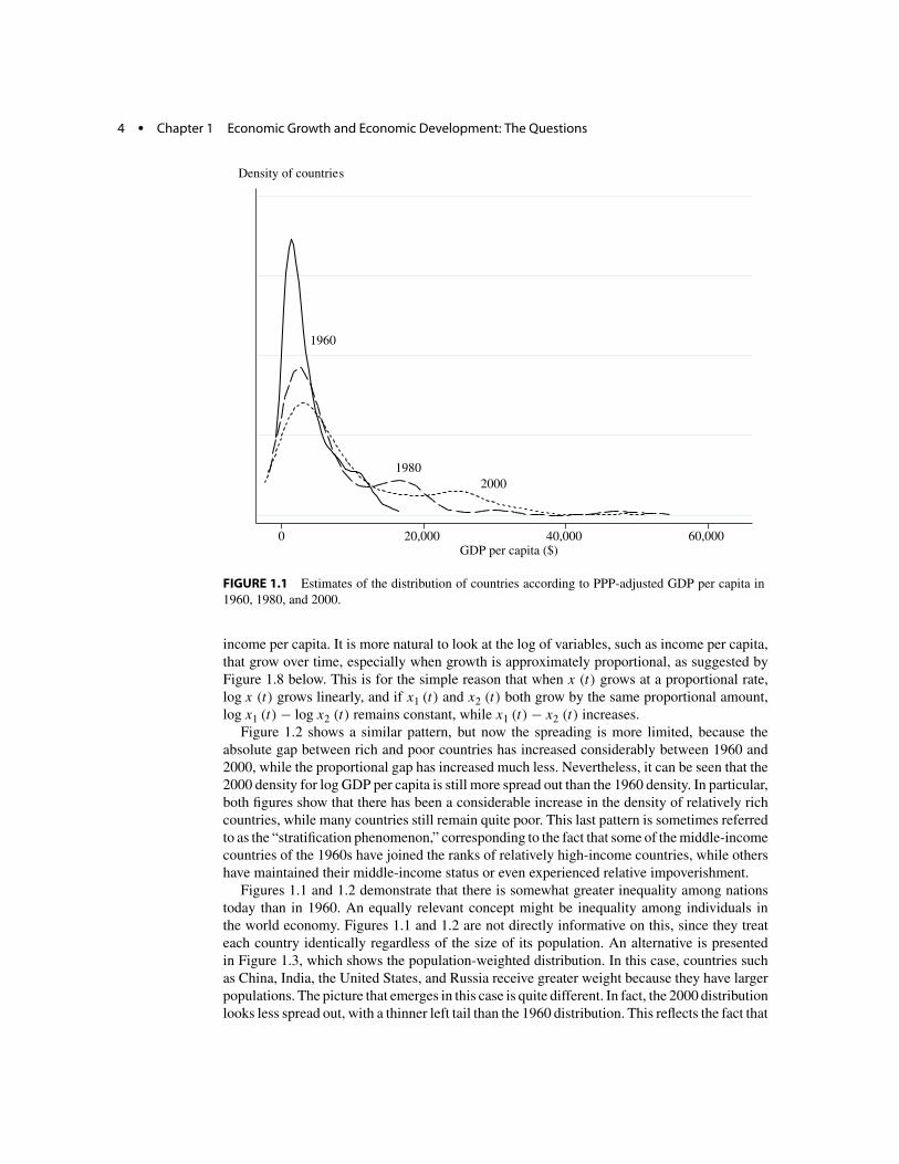
Figure 1.1 provides a first look at these differences. It plots estimates of the distribution of PPP-adjusted GDP per capita across the available set of countries in 1960, 1980, and 2000. A number of features are worth noting. First, the 1960 density shows that 15 years after the end of World War II, most countries had income per capita less than $1,500 (in 2000 U.S. dollars); the mode of the distribution is around $1,250. The rightward shift of the distributions for 1980 and 2000 shows the growth of average income per capita for the next 40 years. In 2000, the mode is slightly above $3,000, but now there is another concentration of countries between $20,000 and $30,000. The density estimate for the year 2000 shows the considerable inequality in income per capita today.
The spreading out of the distribution in Figure 1.1 is partly because of the increase in average incomes. It may therefore be more informative to look at the logarithm (log) of
1. All data are from the Penn World tables compiled by Heston, Summers, and Aten (2002). Details of data sources and more on PPP adjustment can be found in the References and Literature section at the end of this chapter.
3
4 . Chapter 1 Economic Growth and Economic Development: The Questions
Density of countries
1960
1980 2000
0 20,000 40,000 60,000 GDP per capita ($)
FIGURE 1.1 Estimates of the distribution of countries according to PPP-adjusted GDP per capita in 1960, 1980, and 2000.
income per capita. It is more natural to look at the log of variables, such as income per capita, that grow over time, especially when growth is approximately proportional, as suggested by Figure 1.8 below. This is for the simple reason that when x (t) grows at a proportional rate, log x (t) grows linearly, and if x1 (t) and x2 (t) both grow by the same proportional amount, log x1 (t) − log x2 (t) remains constant, while x1 (t) − x2 (t) increases.
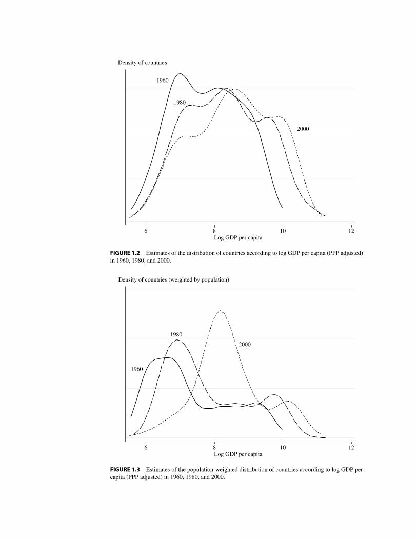
Figure 1.2 shows a similar pattern, but now the spreading is more limited, because the absolute gap between rich and poor countries has increased considerably between 1960 and 2000, while the proportional gap has increased much less. Nevertheless, it can be seen that the 2000 density for log GDP per capita is still more spread out than the 1960 density. In particular, both figures show that there has been a considerable increase in the density of relatively rich countries, while many countries still remain quite poor. This last pattern is sometimes referred to as the “stratification phenomenon,” corresponding to the fact that some of the middle-income countries of the 1960s have joined the ranks of relatively high-income countries, while others have maintained their middle-income status or even experienced relative impoverishment.
Figures 1.1 and 1.2 demonstrate that there is somewhat greater inequality among nations today than in 1960. An equally relevant concept might be inequality among individuals in the world economy. Figures 1.1 and 1.2 are not directly informative on this, since they treat each country identically regardless of the size of its population. An alternative is presented in Figure 1.3, which shows the population-weighted distribution. In this case, countries such as China, India, the United States, and Russia receive greater weight because they have larger populations. The picture that emerges in this case is quite different. In fact, the 2000 distribution looks less spread out, with a thinner left tail than the 1960 distribution. This reflects the fact that
Density of countries
1960
1980
2000
6 8 10 12 Log GDP per capita
FIGURE 1.2 Estimates of the distribution of countries according to log GDP per capita (PPP adjusted) in 1960, 1980, and 2000.
Density of countries (weighted by population)
1960
1980
2000
6 8 10 12 Log GDP per capita
FIGURE 1.3 Estimates of the population-weighted distribution of countries according to log GDP per capita (PPP adjusted) in 1960, 1980, and 2000.
6 . Chapter 1 Economic Growth and Economic Development: The Questions
Density of countries
1960
1980
2000
6 8 10 12 Log GDP per worker
FIGURE 1.4 Estimates of the distribution of countries according to log GDP per worker (PPP adjusted) in 1960, 1980, and 2000.
in 1960 China and India were among the poorest nations in the world, whereas their relatively rapid growth in the 1990s puts them into the middle-poor category by 2000. Chinese and Indian growth has therefore created a powerful force for relative equalization of income per capita among the inhabitants of the globe.
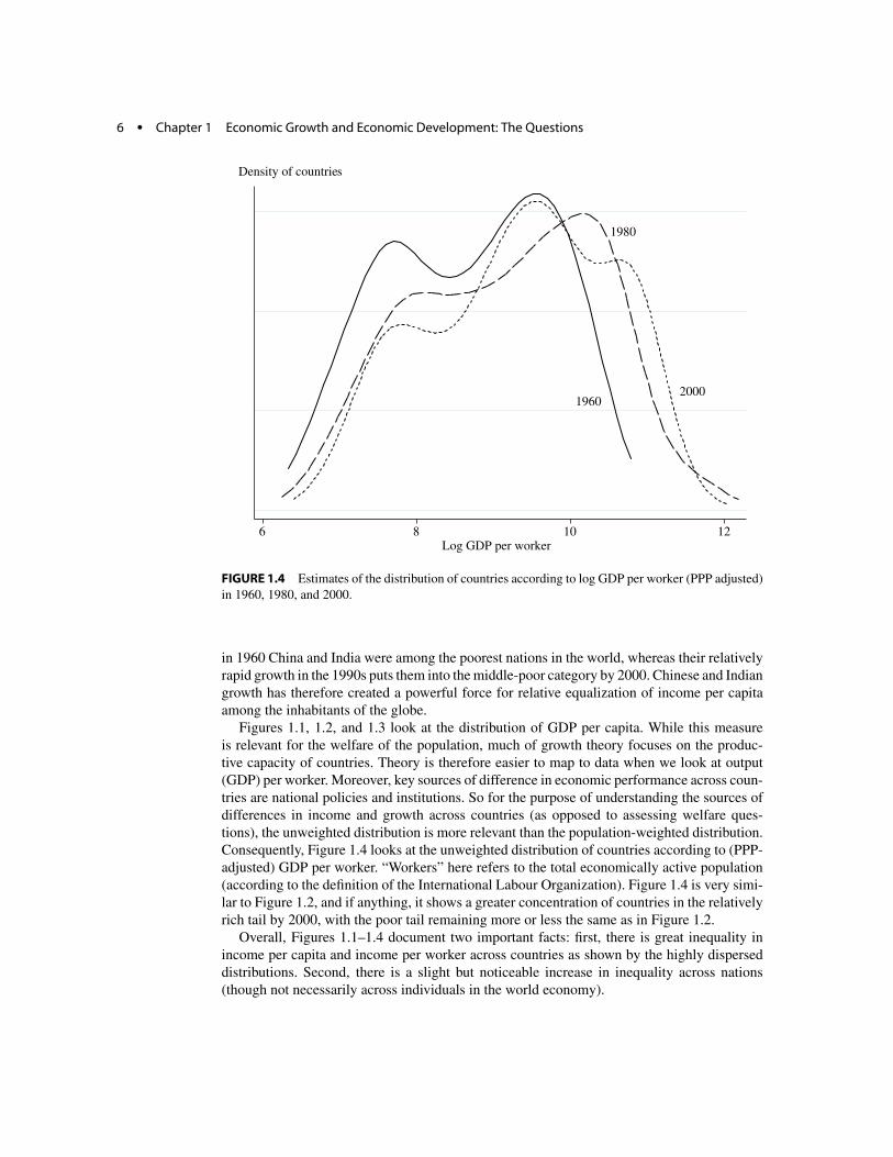
Figures 1.1, 1.2, and 1.3 look at the distribution of GDP per capita. While this measure is relevant for the welfare of the population, much of growth theory focuses on the productive capacity of countries. Theory is therefore easier to map to data when we look at output (GDP) per worker. Moreover, key sources of difference in economic performance across countries are national policies and institutions. So for the purpose of understanding the sources of differences in income and growth across countries (as opposed to assessing welfare questions), the unweighted distribution is more relevant than the population-weighted distribution. Consequently, Figure 1.4 looks at the unweighted distribution of countries according to (PPPadjusted) GDP per worker. “Workers” here refers to the total economically active population (according to the definition of the International Labour Organization). Figure 1.4 is very similar to Figure 1.2, and if anything, it shows a greater concentration of countries in the relatively rich tail by 2000, with the poor tail remaining more or less the same as in Figure 1.2.
Overall, Figures 1.1–1.4 document two important facts: first, there is great inequality in income per capita and income per worker across countries as shown by the highly dispersed distributions. Second, there is a slight but noticeable increase in inequality across nations (though not necessarily across individuals in the world economy).
.1.2 Income and Welfare 7
1.2 Income and Welfare
Should we care about cross-country income differences? The answer is definitely yes. High income levels reflect high standards of living. Economic growth sometimes increases pollution or may raise individual aspirations, so that the same bundle of consumption may no longer satisfy an individual. But at the end of the day, when one compares an advanced, rich country with a less-developed one, there are striking differences in the quality of life, standards of living, and health.
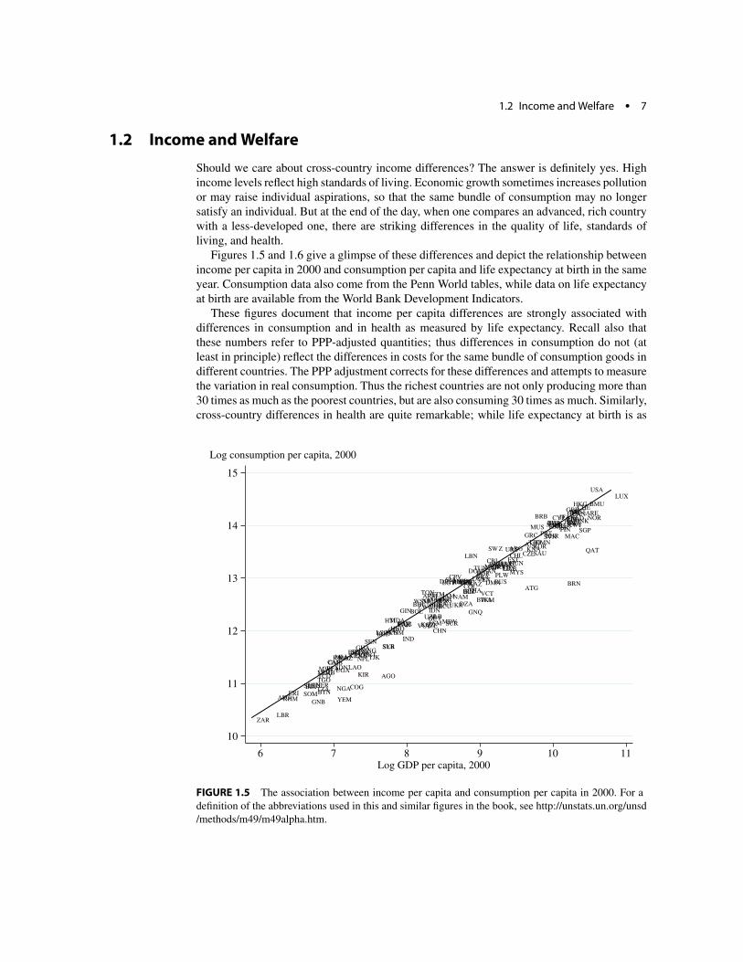
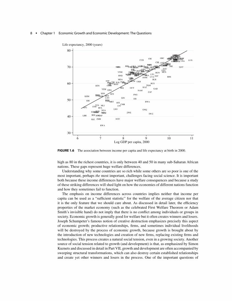
Figures 1.5 and 1.6 give a glimpse of these differences and depict the relationship between income per capita in 2000 and consumption per capita and life expectancy at birth in the same year. Consumption data also come from the Penn World tables, while data on life expectancy at birth are available from the World Bank Development Indicators.
These figures document that income per capita differences are strongly associated with differences in consumption and in health as measured by life expectancy. Recall also that these numbers refer to PPP-adjusted quantities; thus differences in consumption do not (at least in principle) reflect the differences in costs for the same bundle of consumption goods in different countries. The PPP adjustment corrects for these differences and attempts to measure the variation in real consumption. Thus the richest countries are not only producing more than 30 times as much as the poorest countries, but are also consuming 30 times as much. Similarly, cross-country differences in health are quite remarkable; while life expectancy at birth is as
Log consumption per capita, 2000
15
14
13
12
11
10
AFG
ALB
DZA
AGO
ATG
ARG
ARM
AUSAUT
AZE
BHS
BHR
BGD
BRB
BLR
BEL
BLZ
BEN
BMU
BTN
BOL BIH
BWA
BRA BRN
BGR
BFA
BDI
KHM
CMR
CAN
CPV
CAF
TCD
CHL
CHN
COL
COM
ZAR
COG
CRI
CIV
HRV
CUB
CYP
CZE
DNK
DJI DMA
DOM
ECU
EGYSLV
GNQ
ERI
EST
ETH
FJI
FIN
FRA
GAB
GMB
GEO
GER
GHA
GRC
GRD
GTM
GIN
GNB
GUYHTI HND
HKG
HUN
ISL
IND
IDN
IRN
IRQ
IRLISR
ITA
JAM
JPN
JOR
KAZ
KEN
KIR
PRK
KOR
KWT
KGZ
LAO
LVA
LBN
LSO
LBR
LBY LTU
LUX
MAC
MKD
MDGMWI
MYS
MDV
MLI
MLT
MRT
MUS
MEX
FSMMDA
MNG
MAR
MOZ
NAM
NPL
NLD
ANT
NZL
NIC
NER NGA
NOR
OMN
PAK
PLWPAN
PNG
PRY
PERPHL
POL
PRT PRI
QAT
ROM RUS
RWA
WSM
STP
SAU
SEN
SCG
SYC
SLE
SGP
SVK
SVN
SLB
SOM
ZAF
ESP
LKA
KNA
LCA
VCT
SDN
SUR
SW Z
SWE
CHE
SYR
TWN
TJK
TZA
THA
TGO
TON
TTO
TUN
TUR
TKM
UGA
UKR
AREGBR
USA
URY
UZB
VUT
VEN
VNM
YEM
ZMB
ZWE
6 7 8 9 10 11 Log GDP per capita, 2000
FIGURE 1.5 The association between income per capita and consumption per capita in 2000. For a definition of the abbreviations used in this and similar figures in the book, see http://unstats.un.org/unsd /methods/m49/m49alpha.htm.
8 . Chapter 1 Economic Growth and Economic Development: The Questions
Life expectancy, 2000 (years)
AFG
AGO
ALB
ANT
ARE
ARG
ARM
AUS AUT
AZE
BDI
BEL
BEN
BFA
BGD
BGR
BHR
BHS
BIH
BLR
BLZ
BOL
BRA
BRB
BRN
BTN
BWA
CAF
CANCHE
CHL
CHN
CIV CMR
COG
COL
COM
CPV
CRICUB
CYP
CZE
DJI
DNK
DOM
DZA
ECU
EGY
ERI
ESP
EST
FIN
FJI
FRA
FSM
GAB
GBR
GEO
GHA
GIN GMB
GNB GNQ
GRC
GTM
GUY
HKG
HND
HRV
HTI
HUN
IDN
IND
IRL
IRN
IRQ
ISL ISRITA
JAM JOR
JPN
KAZ
KEN
KGZ
KHM
KOR
KWT
LAO
LBN
LBR
LBYLCALKA
LSO
LTU
LUX
LVA
MAC
MAR
MDA
MDG
MDV
MEX MKD
MLI
MLT
MNG
MOZ
MRT
MUS
MWI
MYS
NAM
NER NGA
NIC
NLD NOR
NPL
NZL
OMN
PAK
PAN
PERPHL
PNG
POL
PRI
PRK
PRT
PRY
QAT
ROM
RUS
RWA
SAU SCG
SDN SEN
SGP
SLB
SLE
SLV
SOM
STP
SUR
SVK
SVN
SWE
SW Z
SYR
TCD
TGO
THA
TJK
TKM
TON
TTO
TUN
TUR
TZA
UGA
UKR
URY
USA
UZB
VCT
VEN
VNM
VUTWSM
YEM
ZAF
ZMB
ZWE
ETH
GER
30
40
50
60
70
80
6 7 8 9 10 11 Log GDP per capita, 2000
FIGURE 1.6 The association between income per capita and life expectancy at birth in 2000.
high as 80 in the richest countries, it is only between 40 and 50 in many sub-Saharan African nations. These gaps represent huge welfare differences.
Understanding why some countries are so rich while some others are so poor is one of the most important, perhaps the most important, challenges facing social science. It is important both because these income differences have major welfare consequences and because a study of these striking differences will shed light on how the economies of different nations function and how they sometimes fail to function.
The emphasis on income differences across countries implies neither that income per capita can be used as a “sufficient statistic” for the welfare of the average citizen nor that it is the only feature that we should care about. As discussed in detail later, the efficiency properties of the market economy (such as the celebrated First Welfare Theorem or Adam Smith’s invisible hand) do not imply that there is no conflict among individuals or groups in society. Economic growth is generally good for welfare but it often creates winners and losers. Joseph Schumpeter’s famous notion of creative destruction emphasizes precisely this aspect of economic growth; productive relationships, firms, and sometimes individual livelihoods will be destroyed by the process of economic growth, because growth is brought about by the introduction of new technologies and creation of new firms, replacing existing firms and technologies. This process creates a natural social tension, even in a growing society. Another source of social tension related to growth (and development) is that, as emphasized by Simon Kuznets and discussed in detail in Part VII, growth and development are often accompanied by sweeping structural transformations, which can also destroy certain established relationships and create yet other winners and losers in the process. One of the important questions of
.1.3 Economic Growth and Income Differences 9
political economy, which is discussed in the last part of the book, concerns how institutions and policies can be arranged so that those who lose out from the process of economic growth can be compensated or prevented from blocking economic progress via other means.
A stark illustration of the fact that growth does not always mean an improvement in the living standards of all or even most citizens in a society comes from South Africa under apartheid. Available data (from gold mining wages) suggest that from the beginning of the twentieth century until the fall of the apartheid regime, GDP per capita grew considerably, but the real wages of black South Africans, who make up the majority of the population, likely fell during this period. This of course does not imply that economic growth in South Africa was not beneficial. South Africa is still one of the richest countries in sub-Saharan Africa. Nevertheless, this observation alerts us to other aspects of the economy and also underlines the potential conflicts inherent in the growth process. Similarly, most existing evidence suggests that during the early phases of the British industrial revolution, which started the process of modern economic growth, the living standards of the majority of the workers may have fallen or at best remained stagnant. This pattern of potential divergence between GDP per capita and the economic fortunes of large numbers of individuals and society is not only interesting in and of itself, but it may also inform us about why certain segments of the society may be in favor of policies and institutions that do not encourage growth.
1.3 Economic Growth and Income Differences
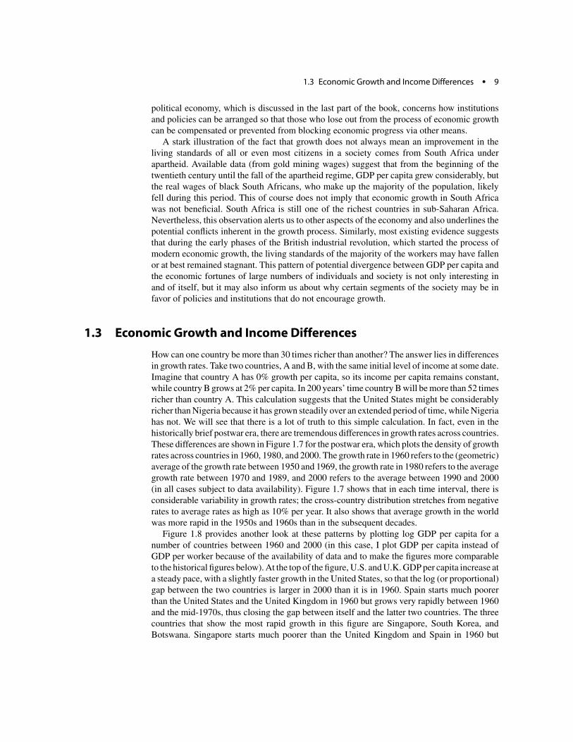
How can one country be more than 30 times richer than another? The answer lies in differences in growth rates. Take two countries, A and B, with the same initial level of income at some date. Imagine that country A has 0% growth per capita, so its income per capita remains constant, while country B grows at 2% per capita. In 200 years’ time country B will be more than 52 times richer than country A. This calculation suggests that the United States might be considerably richer than Nigeria because it has grown steadily over an extended period of time, while Nigeria has not. We will see that there is a lot of truth to this simple calculation. In fact, even in the historically brief postwar era, there are tremendous differences in growth rates across countries. These differences are shown in Figure 1.7 for the postwar era, which plots the density of growth rates across countries in 1960, 1980, and 2000. The growth rate in 1960 refers to the (geometric) average of the growth rate between 1950 and 1969, the growth rate in 1980 refers to the average growth rate between 1970 and 1989, and 2000 refers to the average between 1990 and 2000 (in all cases subject to data availability). Figure 1.7 shows that in each time interval, there is considerable variability in growth rates; the cross-country distribution stretches from negative rates to average rates as high as 10% per year. It also shows that average growth in the world was more rapid in the 1950s and 1960s than in the subsequent decades.
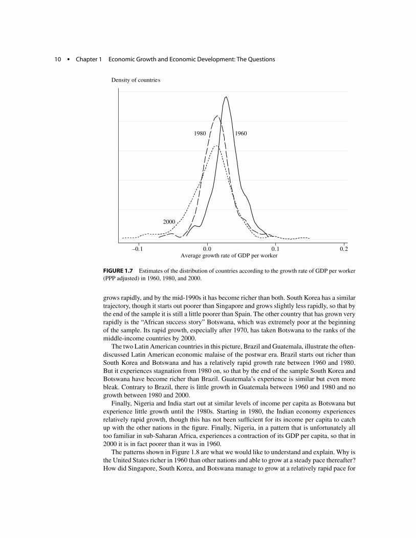
Figure 1.8 provides another look at these patterns by plotting log GDP per capita for a number of countries between 1960 and 2000 (in this case, I plot GDP per capita instead of GDP per worker because of the availability of data and to make the figures more comparable to the historical figures below). At the top of the figure, U.S. and U.K. GDP per capita increase at a steady pace, with a slightly faster growth in the United States, so that the log (or proportional) gap between the two countries is larger in 2000 than it is in 1960. Spain starts much poorer than the United States and the United Kingdom in 1960 but grows very rapidly between 1960 and the mid-1970s, thus closing the gap between itself and the latter two countries. The three countries that show the most rapid growth in this figure are Singapore, South Korea, and Botswana. Singapore starts much poorer than the United Kingdom and Spain in 1960 but
.10 Chapter 1 Economic Growth and Economic Development: The Questions
Density of countries
19601980
2000
–0.1 0.0 0.1 0.2 Average growth rate of GDP per worker
FIGURE 1.7 Estimates of the distribution of countries according to the growth rate of GDP per worker (PPP adjusted) in 1960, 1980, and 2000.
grows rapidly, and by the mid-1990s it has become richer than both. South Korea has a similar trajectory, though it starts out poorer than Singapore and grows slightly less rapidly, so that by the end of the sample it is still a little poorer than Spain. The other country that has grown very rapidly is the “African success story” Botswana, which was extremely poor at the beginning of the sample. Its rapid growth, especially after 1970, has taken Botswana to the ranks of the middle-income countries by 2000.
The two Latin American countries in this picture, Brazil and Guatemala, illustrate the often-discussed Latin American economic malaise of the postwar era. Brazil starts out richer than South Korea and Botswana and has a relatively rapid growth rate between 1960 and 1980. But it experiences stagnation from 1980 on, so that by the end of the sample South Korea and Botswana have become richer than Brazil. Guatemala’s experience is similar but even more bleak. Contrary to Brazil, there is little growth in Guatemala between 1960 and 1980 and no growth between 1980 and 2000.
Finally, Nigeria and India start out at similar levels of income per capita as Botswana but experience little growth until the 1980s. Starting in 1980, the Indian economy experiences relatively rapid growth, though this has not been sufficient for its income per capita to catch up with the other nations in the figure. Finally, Nigeria, in a pattern that is unfortunately all too familiar in sub-Saharan Africa, experiences a contraction of its GDP per capita, so that in 2000 it is in fact poorer than it was in 1960.
The patterns shown in Figure 1.8 are what we would like to understand and explain. Why is the United States richer in 1960 than other nations and able to grow at a steady pace thereafter? How did Singapore, South Korea, and Botswana manage to grow at a relatively rapid pace for
1.4 Today’s Income Differences and World Economic Growth . 11
Log GDP per capita
United States
United Kingdom
Spain
Singapore
Brazil
South Korea
Botswana
Guatemala
Nigeria
India
7
8
9
10
11
1960 1970 1980 1990 2000
FIGURE 1.8 The evolution of income per capita in the United States, the United Kingdom, Spain, Singapore, Brazil, Guatemala, South Korea, Botswana, Nigeria, and India, 1960–2000.
40 years? Why did Spain grow relatively rapidly for about 20 years but then slow down? Why did Brazil and Guatemala stagnate during the 1980s? What is responsible for the disastrous growth performance of Nigeria?
1.4 Origins of Today’s Income Differences and World Economic Growth
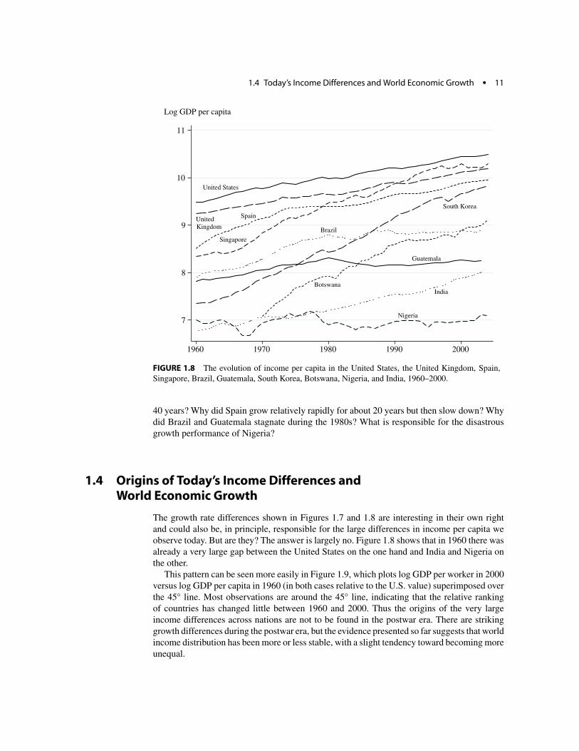
The growth rate differences shown in Figures 1.7 and 1.8 are interesting in their own right and could also be, in principle, responsible for the large differences in income per capita we observe today. But are they? The answer is largely no. Figure 1.8 shows that in 1960 there was already a very large gap between the United States on the one hand and India and Nigeria on the other.
This pattern can be seen more easily in Figure 1.9, which plots log GDP per worker in 2000 versus log GDP per capita in 1960 (in both cases relative to the U.S. value) superimposed over the 45◦ line. Most observations are around the 45◦ line, indicating that the relative ranking of countries has changed little between 1960 and 2000. Thus the origins of the very large income differences across nations are not to be found in the postwar era. There are striking growth differences during the postwar era, but the evidence presented so far suggests that world income distribution has been more or less stable, with a slight tendency toward becoming more unequal.

.12 Chapter 1 Economic Growth and Economic Development: The Questions
Log GDP per worker relative to the United States, 2000
1.1
1.0
0.9
0.8
0.7
0.6
DZA
ARG
AUS AUT
BRB
BEL
BEN
BOL
BRA
BFA
BDI
CMR
CAN
CPV
TCD
CHL
CHN
COL
COMCOG
CRI
CIV
DNK
DOM
ECUEGY
SLV
GNQ
ETH
FIN
FRA
GAB
GMB
GHA
GRC
GTM
GIN
GNB
HND
HKG ISL
IND
IDN
IRN
IRL ISRITA
JAM
JPN
JOR
KEN
KOR
LSO
LUX
MDGMWI
MYS
MLI
MUS
MEX
MAR
MOZ
NPL
NLD
NZL
NIC
NER
NGA
NOR
PAK
PAN
PRY PER
PHL
PRT
ROM
RWA
SEN
SGP
ZAF
ESP
LKA
SWE CHE
SYR
TZA
THA
TGO
TTO
TUR
UGA
GBR
USA
URY
VEN
ZMB
ZWE
0.6 0.7 0.8 0.9 1.0 1.1 Log GDP per worker relative to the United States, 1960
FIGURE 1.9 Log GDP per worker in 2000 versus log GDP per worker in 1960, together with the 45
◦ line.
If not in the postwar era, when did this growth gap emerge? The answer is that much of the divergence took place during the nineteenth and early twentieth centuries. Figures 1.10– 1.12 give a glimpse of these developments by using the data compiled by Angus Maddison for GDP per capita differences across nations going back to 1820 (or sometimes earlier). These data are less reliable than Summers-Heston’s Penn World tables, since they do not come from standardized national accounts. Moreover, the sample is more limited and does not include observations for all countries going back to 1820. Finally, while these data include a correction for PPP, this is less complete than the price comparisons used to construct the price indices in the Penn World tables. Nevertheless, these are the best available estimates for differences in prosperity across a large number of nations beginning in the nineteenth century.
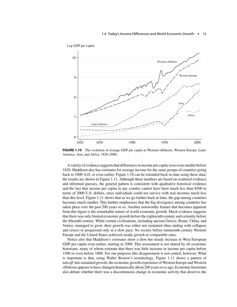
Figure 1.10 illustrates the divergence. It depicts the evolution of average income among five groups of countries: Africa, Asia, Latin America, Western Europe, and Western offshoots of Europe (Australia, Canada, New Zealand, the United States). It shows the relatively rapid growth of the Western offshoots and West European countries during the nineteenth century, while Asia and Africa remained stagnant and Latin America showed little growth. The relatively small (proportional) income gap in 1820 had become much larger by 1960.
Another major macroeconomic fact is visible in Figure 1.10: Western offshoots and West European nations experience a noticeable dip in GDP per capita around 1929 because of the famous Great Depression. Western offshoots, in particular the United States, only recovered fully from this large recession in the wake of World War II. How an economy can experience a sharp decline in output and how it recovers from such a shock are among the major questions of macroeconomics.
1.4 Today’s Income Differences and World Economic Growth . 13
Log GDP per capita
Western offshoots
Western Europe
Africa
Asia
Latin America
6
7
8
9
10
1820 1850 1900 1950 2000
FIGURE 1.10 The evolution of average GDP per capita in Western offshoots, Western Europe, Latin America, Asia, and Africa, 1820–2000.
A variety of evidence suggests that differences in income per capita were even smaller before 1820. Maddison also has estimates for average income for the same groups of countries going back to 1000 A.D. or even earlier. Figure 1.10 can be extended back in time using these data; the results are shown in Figure 1.11. Although these numbers are based on scattered evidence and informed guesses, the general pattern is consistent with qualitative historical evidence and the fact that income per capita in any country cannot have been much less than $500 in terms of 2000 U.S. dollars, since individuals could not survive with real incomes much less than this level. Figure 1.11 shows that as we go further back in time, the gap among countries becomes much smaller. This further emphasizes that the big divergence among countries has taken place over the past 200 years or so. Another noteworthy feature that becomes apparent from this figure is the remarkable nature of world economic growth. Much evidence suggests that there was only limited economic growth before the eighteenth century and certainly before the fifteenth century. While certain civilizations, including ancient Greece, Rome, China, and Venice, managed to grow, their growth was either not sustained (thus ending with collapses and crises) or progressed only at a slow pace. No society before nineteenth-century Western Europe and the United States achieved steady growth at comparable rates.
Notice also that Maddison’s estimates show a slow but steady increase in West European GDP per capita even earlier, starting in 1000. This assessment is not shared by all economic historians, many of whom estimate that there was little increase in income per capita before 1500 or even before 1800. For our purposes this disagreement is not central, however. What is important is that, using Walter Rostow’s terminology, Figure 1.11 shows a pattern of takeoff into sustained growth; the economic growth experience of Western Europe and Western offshoots appears to have changed dramatically about 200 years or so ago. Economic historians also debate whether there was a discontinuous change in economic activity that deserves the
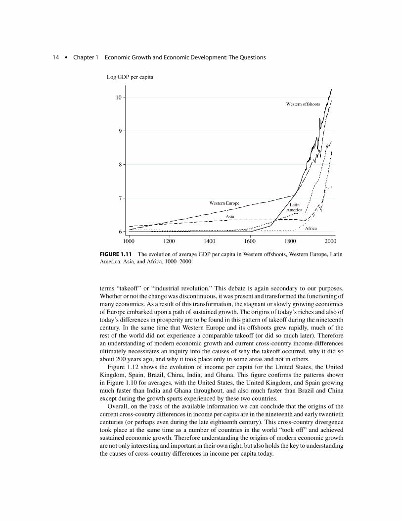
.14 Chapter 1 Economic Growth and Economic Development: The Questions
Log GDP per capita
Western offshoots
Western Europe
Africa
Asia
Latin America
6
7
8
9
10
1000 1200 1400 1600 1800 2000
FIGURE 1.11 The evolution of average GDP per capita in Western offshoots, Western Europe, Latin America, Asia, and Africa, 1000–2000.
terms “takeoff” or “industrial revolution.” This debate is again secondary to our purposes. Whether or not the change was discontinuous, it was present and transformed the functioning of many economies. As a result of this transformation, the stagnant or slowly growing economies of Europe embarked upon a path of sustained growth. The origins of today’s riches and also of today’s differences in prosperity are to be found in this pattern of takeoff during the nineteenth century. In the same time that Western Europe and its offshoots grew rapidly, much of the rest of the world did not experience a comparable takeoff (or did so much later). Therefore an understanding of modern economic growth and current cross-country income differences ultimately necessitates an inquiry into the causes of why the takeoff occurred, why it did so about 200 years ago, and why it took place only in some areas and not in others.
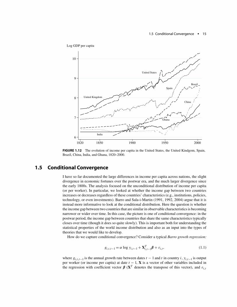
Figure 1.12 shows the evolution of income per capita for the United States, the United Kingdom, Spain, Brazil, China, India, and Ghana. This figure confirms the patterns shown in Figure 1.10 for averages, with the United States, the United Kingdom, and Spain growing much faster than India and Ghana throughout, and also much faster than Brazil and China except during the growth spurts experienced by these two countries.
Overall, on the basis of the available information we can conclude that the origins of the current cross-country differences in income per capita are in the nineteenth and early twentieth centuries (or perhaps even during the late eighteenth century). This cross-country divergence took place at the same time as a number of countries in the world “took off” and achieved sustained economic growth. Therefore understanding the origins of modern economic growth are not only interesting and important in their own right, but also holds the key to understanding the causes of cross-country differences in income per capita today.
1.5 Conditional Convergence . 15
Log GDP per capita
United Kingdom
United States
Spain
China
Brazil
India
Ghana
6
7
8
9
10
1820 1850 1900 1950 2000
FIGURE 1.12 The evolution of income per capita in the United States, the United Kindgom, Spain, Brazil, China, India, and Ghana, 1820–2000.
1.5 Conditional Convergence
I have so far documented the large differences in income per capita across nations, the slight divergence in economic fortunes over the postwar era, and the much larger divergence since the early 1800s. The analysis focused on the unconditional distribution of income per capita (or per worker). In particular, we looked at whether the income gap between two countries increases or decreases regardless of these countries’ characteristics (e.g., institutions, policies, technology, or even investments). Barro and Sala-i-Martin (1991, 1992, 2004) argue that it is instead more informative to look at the conditional distribution. Here the question is whether the income gap between two countries that are similar in observable characteristics is becoming narrower or wider over time. In this case, the picture is one of conditional convergence: in the postwar period, the income gap between countries that share the same characteristics typically closes over time (though it does so quite slowly). This is important both for understanding the statistical properties of the world income distribution and also as an input into the types of theories that we would like to develop.
How do we capture conditional convergence? Consider a typical Barro growth regression:
gi,t,t−1 = α log yi,t−1 + XT (1.1)i,t−1β + εi,t ,
where gi,t,t−1 is the annual growth rate between dates t − 1 and t in country i, yi,t−1 is output per worker (or income per capita) at date t − 1, X is a vector of other variables included in the regression with coefficient vector β (XT denotes the transpose of this vector), and εi,t
.16 Chapter 1 Economic Growth and Economic Development: The Questions
Average growth rate of GDP, 1960–2000
0.06
0.04
0.02
0.00
–0.02
TWN
CHN GNQ KOR
HKG
THA MYS ROM JPN SGP
IRL
LKA LUX
GHA LSO PAK
PRT ESP AUT
IND GRC IDN CPV MUS ISRBELEGY ITA
TUR FRAMAR FIN NOR
PANSYR
DOM GBR MWI NPL
BRA ISL
DNK USA
GAB NLD
TZA CIV PHL PRY IRN CHL
TTO SWE
CANCHE
ETH AUS GNB
BFA BEN COL MEX BRBZWE ECU ZAF
URY GMB COG CRI ARGMLI CMR GTMMOZ
UGA DZA NZL
HND BOL SLV BDI
ZMB NGA PER
TGO KEN JAMRWA COM SEN
GIN VEN
TCD JOR NER
MDG NIC
7 8 9 10 11 Log GDP per worker, 1960
FIGURE 1.13 Annual growth rate of GDP per worker between 1960 and 2000 versus log GDP per worker in 1960 for the entire world.
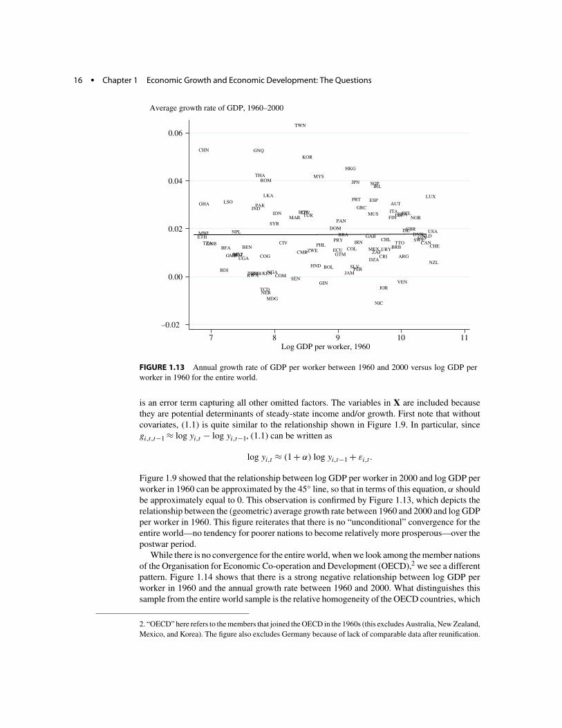
is an error term capturing all other omitted factors. The variables in X are included because they are potential determinants of steady-state income and/or growth. First note that without covariates, (1.1) is quite similar to the relationship shown in Figure 1.9. In particular, since gi,t,t−1 ≈ log yi,t − log yi,t−1, (1.1) can be written as
log yi,t ≈ (1 + α) log yi,t−1 + εi,t .
Figure 1.9 showed that the relationship between log GDP per worker in 2000 and log GDP per worker in 1960 can be approximated by the 45◦ line, so that in terms of this equation, α should be approximately equal to 0. This observation is confirmed by Figure 1.13, which depicts the relationship between the (geometric) average growth rate between 1960 and 2000 and log GDP per worker in 1960. This figure reiterates that there is no “unconditional” convergence for the entire world—no tendency for poorer nations to become relatively more prosperous—over the postwar period.
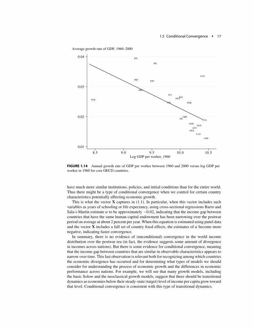
While there is no convergence for the entire world, when we look among the member nations of the Organisation for Economic Co-operation and Development (OECD),2 we see a different pattern. Figure 1.14 shows that there is a strong negative relationship between log GDP per worker in 1960 and the annual growth rate between 1960 and 2000. What distinguishes this sample from the entire world sample is the relative homogeneity of the OECD countries, which
2. “OECD” here refers to the members that joined the OECD in the 1960s (this excludes Australia, New Zealand, Mexico, and Korea). The figure also excludes Germany because of lack of comparable data after reunification.
1.5 Conditional Convergence . 17
Average growth rate of GDP, 1960–2000
AUS
BEL
CAN
DNK
FIN
FRA
GRC
ISL
IRL
ITA
JPN
LUX
NLD
NOR
PRT ESP
SWE
CHE
TUR
GBR
USA
0.01
0.02
0.03
0.04
8.5 9.0 9.5 10. 0 10. 5 Log GDP per worker, 1960
FIGURE 1.14 Annual growth rate of GDP per worker between 1960 and 2000 versus log GDP per worker in 1960 for core OECD countries.
have much more similar institutions, policies, and initial conditions than for the entire world. Thus there might be a type of conditional convergence when we control for certain country characteristics potentially affecting economic growth.
This is what the vector X captures in (1.1). In particular, when this vector includes such variables as years of schooling or life expectancy, using cross-sectional regressions Barro and Sala-i-Martin estimate α to be approximately −0.02, indicating that the income gap between countries that have the same human capital endowment has been narrowing over the postwar period on average at about 2 percent per year. When this equation is estimated using panel data and the vector X includes a full set of country fixed effects, the estimates of α become more negative, indicating faster convergence.
In summary, there is no evidence of (unconditional) convergence in the world income distribution over the postwar era (in fact, the evidence suggests some amount of divergence in incomes across nations). But there is some evidence for conditional convergence, meaning that the income gap between countries that are similar in observable characteristics appears to narrow over time. This last observation is relevant both for recognizing among which countries the economic divergence has occurred and for determining what types of models we should consider for understanding the process of economic growth and the differences in economic performance across nations. For example, we will see that many growth models, including the basic Solow and the neoclassical growth models, suggest that there should be transitional dynamics as economies below their steady-state (target) level of income per capita grow toward that level. Conditional convergence is consistent with this type of transitional dynamics.
.18 Chapter 1 Economic Growth and Economic Development: The Questions
1.6 Correlates of Economic Growth
The previous section emphasized the importance of certain country characteristics that might be related to the process of economic growth. What types of countries grow more rapidly? Ideally, this question should be answered at a causal level. In other words, we would like to know which specific characteristics of countries (including their policies and institutions) have a causal effect on growth. “Causal effect” refers to the answer to the following counterfactual thought experiment: if, all else being equal, a particular characteristic of the country were changed exogenously (i.e., not as part of equilibrium dynamics or in response to a change in other observable or unobservable variables), what would be the effect on equilibrium growth? Answering such causal questions is quite challenging, precisely because it is difficult to isolate changes in endogenous variables that are not driven by equilibrium dynamics or by omitted factors.
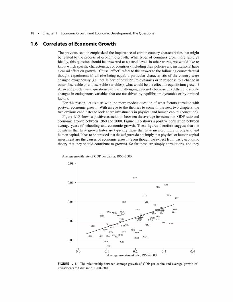
For this reason, let us start with the more modest question of what factors correlate with postwar economic growth. With an eye to the theories to come in the next two chapters, the two obvious candidates to look at are investments in physical and human capital (education).
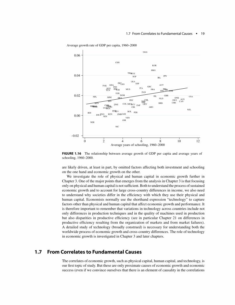
Figure 1.15 shows a positive association between the average investment to GDP ratio and economic growth between 1960 and 2000. Figure 1.16 shows a positive correlation between average years of schooling and economic growth. These figures therefore suggest that the countries that have grown faster are typically those that have invested more in physical and human capital. It has to be stressed that these figures do not imply that physical or human capital investment are the causes of economic growth (even though we expect from basic economic theory that they should contribute to growth). So far these are simply correlations, and they
Average growth rate of GDP per capita, 1960–2000
ARG
AUS
AUT BEL
BEN
BOL
BRA
BFA
CANCHL
CHN
COL
CRI
DNK
DOM
ECU
EGY
SLV
ETH
FINFRA
GHA
GRC
GTM
GIN
HND
ISLIND
IRN
IRL
ISRITA
JAM
JPN
JOR
KEN
KOR
LUX
MWI
MYS
MUS
MEX
MAR NLD
NZL
NIC
NGA
NOR
PAK
PAN
PRY
PER
PHL
PRT
ZAF
ESP
LKA
SW E
CHE
TWN
THA
TTO TUR
UGA
GBR USA
URY
VENZMB
ZWE
0.00
0.02
0.04
0.06
0.08
0.0 0.1 0.2 0.3 0.4 Average investment rate, 1960–2000
FIGURE 1.15 The relationship between average growth of GDP per capita and average growth of investments to GDP ratio, 1960–2000.
1.7 From Correlates to Fundamental Causes . 19
Average growth rate of GDP per capita, 1960–2000
0.06
0.04
0.02
0.00
–0.02
TWN
CHN
RWA
KOR
HKG
THAMYS
SGP IRL
JPN
LKA
EGY IDN
PAK GHA LSO IND
PRT
SYR
TUN TUR MUS
ESP
ITA
PAN FRA
GRC AUT
BEL FIN NORISR
BDI
BEN
MLIGMBMOZ
NPL
SLV BOL PER
MWI BRA
CMR ZAF COG
ZWE COL MEXECU
UGADZA CRI
DOM
GTM
HND
IRN
TGO KEN ZMBJAM
PRY
ARG
CHL
ISL
PHLTTO URY BRB
NLD
GBR
AUS CAN
CHE
DNK SWE
NZL
USA
SEN VEN
JOR NER
NIC
0 2 4 6 8 10 12 Average years of schooling, 1960–2000
FIGURE 1.16 The relationship between average growth of GDP per capita and average years of schooling, 1960–2000.
are likely driven, at least in part, by omitted factors affecting both investment and schooling on the one hand and economic growth on the other.
We investigate the role of physical and human capital in economic growth further in Chapter 3. One of the major points that emerges from the analysis in Chapter 3 is that focusing only on physical and human capital is not sufficient. Both to understand the process of sustained economic growth and to account for large cross-country differences in income, we also need to understand why societies differ in the efficiency with which they use their physical and human capital. Economists normally use the shorthand expression “technology” to capture factors other than physical and human capital that affect economic growth and performance. It is therefore important to remember that variations in technology across countries include not only differences in production techniques and in the quality of machines used in production but also disparities in productive efficiency (see in particular Chapter 21 on differences in productive efficiency resulting from the organization of markets and from market failures). A detailed study of technology (broadly construed) is necessary for understanding both the worldwide process of economic growth and cross-country differences. The role of technology in economic growth is investigated in Chapter 3 and later chapters.
1.7 From Correlates to Fundamental Causes
The correlates of economic growth, such as physical capital, human capital, and technology, is our first topic of study. But these are only proximate causes of economic growth and economic success (even if we convince ourselves that there is an element of causality in the correlations
.20 Chapter 1 Economic Growth and Economic Development: The Questions
shown above). It would not be entirely satisfactory to explain the process of economic growth and cross-country differences with technology, physical capital, and human capital, since presumably there are reasons technology, physical capital, and human capital differ across countries. If these factors are so important in generating cross-country income differences and causing the takeoff into modern economic growth, why do certain societies fail to improve their technologies, invest more in physical capital, and accumulate more human capital?
Let us return to Figure 1.8 to illustrate this point further. This figure shows that South Korea and Singapore have grown rapidly over the past 50 years, while Nigeria has failed to do so. We can try to explain the successful performances of South Korea and Singapore by looking at the proximate causes of economic growth. We can conclude, as many have done, that rapid capital accumulation has been a major cause of these growth miracles and debate the relative roles of human capital and technology. We can simply blame the failure of Nigeria to grow on its inability to accumulate capital and to improve its technology. These perspectives are undoubtedly informative for understanding the mechanics of economic successes and failures of the postwar era. But at some level they do not provide answers to the central questions: How did South Korea and Singapore manage to grow, while Nigeria failed to take advantage of its growth opportunities? If physical capital accumulation is so important, why did Nigeria fail to invest more in physical capital? If education is so important, why are education levels in Nigeria still so low, and why is existing human capital not being used more effectively? The answer to these questions is related to the fundamental causes of economic growth—the factors potentially affecting why societies make different technology and accumulation choices.
At some level, fundamental causes are the factors that enable us to link the questions of economic growth to the concerns of the rest of the social sciences and ask questions about the roles of policies, institutions, culture, and exogenous environmental factors. At the risk of oversimplifying complex phenomena, we can think of the following list of potential fundamental causes: (1) luck (or multiple equilibria) that lead to divergent paths among societies with identical opportunities, preferences, and market structures; (2) geographic differences that affect the environment in which individuals live and influence the productivity of agriculture, the availability of natural resources, certain constraints on individual behavior, or even individual attitudes; (3) institutional differences that affect the laws and regulations under which individuals and firms function and shape the incentives they have for accumulation, investment, and trade; and (4) cultural differences that determine individuals’ values, preferences, and beliefs. Chapter 4 presents a detailed discussion of the distinction between proximate and fundamental causes and what types of fundamental causes are more promising in explaining the process of economic growth and cross-country income differences.
For now, it is useful to briefly return to the contrast between South Korea and Singapore versus Nigeria and ask the questions (even if we are not in a position to fully answer them yet): Can we say that South Korea and Singapore owe their rapid growth to luck, while Nigeria was unlucky? Can we relate the rapid growth of South Korea and Singapore to geographic factors? Can we relate them to institutions and policies? Can we find a major role for culture? Most detailed accounts of postwar economics and politics in these countries emphasize the role of growth-promoting policies in South Korea and Singapore—including the relative security of property rights and investment incentives provided to firms. In contrast, Nigeria’s postwar history is one of civil war, military coups, endemic corruption, and overall an environment that failed to provide incentives to businesses to invest and upgrade their technologies. It therefore seems necessary to look for fundamental causes of economic growth that make contact with these facts. Jumping ahead a little, it already appears implausible that luck can be the major explanation for the differences in postwar economic performance; there were already significant economic differences between South Korea, Singapore, and Nigeria at the beginning of the postwar era. It is also equally implausible to link the divergent fortunes of these countries

.1.8 The Agenda 21
to geographic factors. After all, their geographies did not change, but the growth spurts of South Korea and Singapore started in the postwar era. Moreover, even if Singapore benefited from being an island, without hindsight one might have concluded that Nigeria had the best environment for growth because of its rich oil reserves.3 Cultural differences across countries are likely to be important in many respects, and the rapid growth of many Asian countries is often linked to certain “Asian values.” Nevertheless, cultural explanations are also unlikely to adequately explain fundamental causes, since South Korean or Singaporean culture did not change much after the end of World War II, while their rapid growth is a distinctly postwar phenomenon. Moreover, while South Korea grew rapidly, North Korea, whose inhabitants share the same culture and Asian values, has endured one of the most disastrous economic performances of the past 50 years.
This admittedly quick (and partial) account suggests that to develop a better understanding of the fundamental causes of economic growth, we need to look at institutions and policies that affect the incentives to accumulate physical and human capital and improve technology. Institutions and policies were favorable to economic growth in South Korea and Singapore, but not in Nigeria. Understanding the fundamental causes of economic growth is largely about understanding the impact of these institutions and policies on economic incentives and why, for example, they have enhanced growth in South Korea and Singapore but not in Nigeria. The intimate link between fundamental causes and institutions highlighted by this discussion motivates Part VIII, which is devoted to the political economy of growth, that is, to the study of how institutions affect growth and why they differ across countries.
An important caveat should be noted at this point. Discussions of geography, institutions, and culture can sometimes be carried out without explicit reference to growth models or even to growth empirics. After all, this is what many social scientists do outside the field of economics. However, fundamental causes can only have a big impact on economic growth if they affect parameters and policies that have a first-order influence on physical and human capital and technology. Therefore an understanding of the mechanics of economic growth is essential for evaluating whether candidate fundamental causes of economic growth could indeed play the role that is sometimes ascribed to them. Growth empirics plays an equally important role in distinguishing among competing fundamental causes of cross-country income differences. It is only by formulating parsimonious models of economic growth and confronting them with data that we can gain a better understanding of both the proximate and the fundamental causes of economic growth.
1.8 The Agenda
The three major questions that have emerged from the brief discussion are:
1. Why are there such large differences in income per capita and worker productivity across countries?
2. Why do some countries grow rapidly while other countries stagnate?
3. What sustains economic growth over long periods of time, and why did sustained growth start 200 years or so ago?
3. One can turn this reasoning around and argue that Nigeria is poor because of a “natural resource curse,” that is, precisely because it has abundant natural resources. But this argument is not entirely compelling, since there are other countries, such as Botswana, with abundant natural resources that have grown rapidly over the past 50 years. More important, the only plausible channel through which abundance of natural resources may lead to worse economic outcomes is related to institutional and political economy factors. Such factors take us to the realm of institutional fundamental causes.
.22 Chapter 1 Economic Growth and Economic Development: The Questions
For each question, a satisfactory answer requires a set of well-formulated models that illustrate the mechanics of economic growth and cross-country income differences together with an investigation of the fundamental causes of the different trajectories which these nations have embarked upon. In other words, we need a combination of theoretical models and empirical work.
The traditional growth models—in particular, the basic Solow and the neoclassical models— provide a good starting point, and the emphasis they place on investment and human capital seems consistent with the patterns shown in Figures 1.15 and 1.16. However, we will also see that technological differences across countries (either because of their differential access to technological opportunities or because of differences in the efficiency of production) are equally important. Traditional models treat technology and market structure as given or at best as evolving exogenously (rather like a black box). But if technology is so important, we ought to understand why and how it progresses and why it differs across countries. This motivates our detailed study of endogenous technological progress and technology adoption. Specifically, we will try to understand how differences in technology may arise, persist, and contribute to differences in income per capita. Models of technological change are also useful in thinking about the sources of sustained growth of the world economy over the past 200 years and the reasons behind the growth process that took off 200 years or so ago and has proceeded relatively steadily ever since.
Some of the other patterns encountered in this chapter will inform us about the types of models that have the greatest promise in explaining economic growth and cross-country differences in income. For example, we have seen that cross-country income differences can be accounted for only by understanding why some countries have grown rapidly over the past 200 years while others have not. Therefore we need models that can explain how some countries can go through periods of sustained growth while others stagnate.
Nevertheless, we have also seen that the postwar world income distribution is relatively stable (at most spreading out slightly from 1960 to 2000). This pattern has suggested to many economists that we should focus on models that generate large permanent cross-country differences in income per capita but not necessarily large permanent differences in growth rates (at least not in the recent decades). This argument is based on the following reasoning: with substantially different long-run growth rates (as in models of endogenous growth, where countries that invest at different rates grow at permanently different rates), we should expect significant divergence. We saw above that despite some widening between the top and the bottom, the cross-country distribution of income across the world is relatively stable over the postwar era.
Combining the postwar patterns with the origins of income differences over the past several centuries suggests that we should look for models that can simultaneously account for long periods of significant growth differences and for a distribution of world income that ultimately becomes stationary, though with large differences across countries. The latter is particularly challenging in view of the nature of the global economy today, which allows for the free flow of technologies and large flows of money and commodities across borders. We therefore need to understand how the poor countries fell behind and what prevents them today from adopting and imitating the technologies and the organizations (and importing the capital) of richer nations.
And as the discussion in the previous section suggests, all of these questions can be (and perhaps should be) answered at two distinct but related levels (and in two corresponding steps). The first step is to use theoretical models and data to understand the mechanics of economic growth. This step sheds light on the proximate causes of growth and explains differences in income per capita in terms of differences in physical capital, human capital, and technology,
.1.9 References and Literature 23
and these in turn will be related to other variables, such as preferences, technology, market structure, openness to international trade, and economic policies.
The second step is to look at the fundamental causes underlying these proximate factors and investigate why some societies are organized differently than others. Why do societies have different market structures? Why do some societies adopt policies that encourage economic growth while others put up barriers to technological change? These questions are central to a study of economic growth and can only be answered by developing systematic models of the political economy of development and looking at the historical process of economic growth to generate data that can shed light on these fundamental causes.
Our next task is to systematically develop a series of models to understand the mechanics of economic growth. I present a detailed exposition of the mathematical structure of a number of dynamic general equilibrium models that are useful for thinking about economic growth and related macroeconomic phenomena, and I emphasize the implications of these models for the sources of differences in economic performance across societies. Only by understanding these mechanics can we develop a useful framework for thinking about the causes of economic growth and income disparities.
1.9 References and Literature
The empirical material presented in this chapter is largely standard, and parts of it can be found in many books, though interpretations and emphases differ. Excellent introductions, with slightly different emphases, are provided in Jones’s (1998, Chapter 1) and Weil’s (2005, Chapter 1) undergraduate economic growth textbooks. Barro and Sala-i-Martin (2004) also present a brief discussion of the stylized facts of economic growth, though their focus is on postwar growth and conditional convergence rather than the very large cross-country income differences and the long-run perspective stressed here. Excellent and very readable accounts of the key questions of economic growth, with a similar perspective to the one here, are provided in Helpman (2005) and in Aghion and Howitt’s new book (2008). Aghion and Howitt also provide a very useful introduction to many of the same topics discussed in this book.
Much of the data used in this chapter come from Summers-Heston’s (Penn World) dataset (latest version, Summers, Heston, and Aten, 2006). These tables are the result of a careful study by Robert Summers and Alan Heston to construct internationally comparable price indices and estimates of income per capita and consumption. PPP adjustment is made possible by these data. Summers and Heston (1991) give a lucid discussion of the methodology for PPP adjustment and its use in the Penn World tables. PPP adjustment enables the construction of measures of income per capita that are comparable across countries. Without PPP adjustment, differences in income per capita across countries can be computed using the current exchange rate or some fundamental exchange rate. There are many problems with such exchange rate– based measures, however. The most important one is that they do not allow for the marked differences in relative prices and even overall price levels across countries. PPP adjustment brings us much closer to differences in real income and real consumption. GDP, consumption, and investment data from the Penn World tables are expressed in 1996 constant U.S. dollars. Information on workers (economically active population), consumption, and investment are also from this dataset. Life expectancy data are from the World Bank’s World Development Indicators CD-ROM and refer to the average life expectancy of males and females at birth. This dataset also contains a range of other useful information. Schooling data are from Barro and Lee’s (2001) dataset, which contains internationally comparable information on years of schooling. Throughout, cross-country figures use the World Bank labels to denote the identity
.24 Chapter 1 Economic Growth and Economic Development: The Questions
of individual countries. A list of the labels can be found in http://unstats.un.org/unsd/methods/ m49/m49alpha.htm.
In all figures and regressions, growth rates are computed as geometric averages. In particular, the geometric average growth rate of output per capita y between date t and t + T is
� �1/T
gt,t+T ≡ yt+T − 1. yt
The geometric average growth rate is more appropriate to use in the context of income per capita than is the arithmetic average, since the growth rate refers to proportional growth. It can be easily verified from this formula that if yt+1 = (1 + g) yt for all t , then gt+T = g.
Historical data are from various works by Angus Maddison, in particular, Maddison (2001, 2003). While these data are not as reliable as the estimates from the Penn World tables, the general patterns they show are typically consistent with evidence from a variety of different sources. Nevertheless, there are points of contention. For example, in Figure 1.11 Maddison’s estimates show a slow but relatively steady growth of income per capita in Western Europe starting in 1000. This growth pattern is disputed by some historians and economic historians. A relatively readable account, which strongly disagrees with this conclusion, is provided in Pomeranz (2000), who argues that income per capita in Western Europe and the Yangtze Valley in China were broadly comparable as late as 1800. This view also receives support from recent research by Allen (2004), which documents that the levels of agricultural productivity in 1800 were comparable in Western Europe and China. Acemoglu, Johnson, and Robinson (2002, 2005b) use urbanization rates as a proxy for income per capita and obtain results that are intermediate between those of Maddison and Pomeranz. The data in Acemoglu, Johnson, and Robinson (2002) also confirm that there were very limited income differences across countries as late as the 1500s and that the process of rapid economic growth started in the nineteenth century (or perhaps in the late eighteenth century). Recent research by Broadberry and Gupta (2006) also disputes Pomeranz’s arguments and gives more support to a pattern in which there was already an income gap between Western Europe and China by the end of the eighteenth century.
The term “takeoff” used in Section 1.4 is introduced in Walter Rostow’s famous book The Stages of Economic Growth (1960) and has a broader connotation than the term “industrial revolution,” which economic historians typically use to refer to the process that started in Britain at the end of the eighteenth century (e.g., Ashton, 1969). Mokyr (1993) contains an excellent discussion of the debate on whether the beginning of industrial growth was due to a continuous or discontinuous change. Consistent with my emphasis here, Mokyr concludes that this is secondary to the more important fact that the modern process of growth did start around this time.
There is a large literature on the correlates of economic growth, starting with Barro (1991). This work is surveyed in Barro and Sala-i-Martin (2004) and Barro (1997). Much of this literature, however, interprets these correlations as causal effects, even when this interpretation is not warranted (see the discussions in Chapters 3 and 4).
Note that Figures 1.15 and 1.16 show the relationship between average investment and average schooling between 1960 and 2000 and economic growth over the same period. The relationship between the growth of investment and economic growth over this time is similar, but there is a much weaker relationship between growth of schooling and economic growth. This lack of association between growth of schooling and growth of output may be for a number of reasons. First, there is considerable measurement error in schooling estimates (see Krueger and Lindahl, 2001). Second, as shown in some of the models discussed later, the main role of human capital may be to facilitate technology adoption, and thus we may expect a stronger
1.9 References and Literature . 25
relationship between the level of schooling and economic growth than between the change in schooling and economic growth (see Chapter 10). Finally, the relationship between the level of schooling and economic growth may be partly spurious, in the sense that it may be capturing the influence of some other omitted factors also correlated with the level of schooling; if this is the case, these omitted factors may be removed when we look at changes. While we cannot reach a firm conclusion on these alternative explanations, the strong correlation between average schooling and economic growth documented in Figure 1.16 is interesting in itself.
The narrowing of differences in income per capita in the world economy when countries are weighted by population is explored in Sala-i-Martin (2005). Deaton (2005) contains a critique of Sala-i-Martin’s approach. The point that incomes must have been relatively equal around 1800 or before, because there is a lower bound on real incomes necessary for the survival of an individual, was first made by Maddison (1991), and was later popularized by Pritchett (1997). Maddison’s estimates of GDP per capita and Acemoglu, Johnson, and Robinson’s (2002) estimates based on urbanization confirm this conclusion.
The estimates of the density of income per capita reported in this chapter are similar to those used by Quah (1993, 1997) and Jones (1997). These estimates use a nonparametric Gaussian kernel. The specific details of the kernel estimation do not change the general shape of the densities. Quah was also the first to emphasize the stratification in the world income distribution and the possible shift toward a bimodal distribution, which is visible in Figure 1.3. He dubbed this the “Twin Peaks” phenomenon (see also Durlauf and Quah, 1999). Barro (1991) and Barro and Sala-i-Martin (1992, 2004) emphasize the presence and importance of conditional convergence and argue against the relevance of the stratification pattern emphasized by Quah and others. The estimate of conditional convergence of about 2% per year is from Barro and Sala-i-Martin (1992). Caselli, Esquivel, and Lefort (1996) show that panel data regressions lead to considerably higher rates of conditional convergence.
Marris (1982) and Baumol (1986) were the first economists to conduct cross-country studies of convergence. However, the data at the time were of lower quality than the Summers-Heston data and also were available for only a selected sample of countries. Barro’s (1991) and Barro and Sala-i-Martin’s (1992) work using the Summers-Heston dataset has been instrumental in generating renewed interest in cross-country growth regressions.
The data on GDP growth and black real wages in South Africa are from Wilson (1972). Wages refer to real wages in gold mines. Feinstein (2005) provides an excellent economic history of South Africa. The implications of the British industrial revolution for real wages and living standards of workers are discussed in Mokyr (1993). Another example of rapid economic growth with falling real wages is provided by the experience of the Mexican economy in the early twentieth century (see Gomez-Galvarriato, 1998). There is also evidence that during this period, the average height of the population might have been declining, which is often associated with falling living standards (see Lopez-Alonso and Porras Condey, 2004).
There is a major debate on the role of technology and capital accumulation in the growth experiences of East Asian nations, particularly South Korea and Singapore. See Young (1991, 1995) for the argument that increases in physical capital and labor inputs explain almost all of the rapid growth in these two countries. See Klenow and Rodriguez (1997) and Hsieh (2002) for the opposite point of view.
The difference between proximate and fundamental causes is discussed further in later chapters. This distinction is emphasized in a different context by Diamond (1997), though it is also implicitly present in North and Thomas’s (1973) classic book. It is discussed in detail in the context of long-run economic development and economic growth in Acemoglu, Johnson, and Robinson (2005a). I revisit these issues in greater detail in Chapter 4.