DATA STRUCTURESFOR LOGIC OPTIMIZATION

c©Giovanni De Micheli

Stanford University

Outline

c© GDM

• Review of Boolean algebra.

• Representations of logic functions.

• Matrix representations of covers.

• Operations on logic covers.

Background

c© GDM

• Function f(x1, x2, . . . , xi, . . . , xn).

• Cofactor of f with respect to variable xi:

– fxi ≡ f(x1, x2, . . . ,1, . . . , xn).

• Cofactor of f with respect to variable x′i:

– fx′i≡ f(x1, x2, . . . ,0, . . . , xn).

• Boole’s expansion theorem:

– f(x1, x2, . . . , xi, . . . , xn) = xi·fxi+x′i·fx′i

Example

c© GDM

• Function:f = ab + bc + ac

• Cofactors:

– fa = b + c

– fa′ = bc

• Expansion:

– f = afa + a′fa′ = a(b + c) + a′bc

Background

c© GDM

• Function f(x1, x2, . . . , xi, . . . , xn).

• Positive unate in xi when:

– fxi ≥ fx′i

• Negative unate in xi when:

– fxi ≤ fx′i

• A function is positive/negative unate when

positive/negative unate in all its variables.

Background

c© GDM

• Function f(x1, x2, . . . , xi, . . . , xn).

• Boolean difference of f w.r.t. variable xi:

– ∂f/∂xi ≡ fxi ⊕ fx′i.

• Consensus of f w. r. to variable xi:

– Cxi ≡ fxi · fx′i.

• Smoothing of f w. r. to variable xi:

– Sxi ≡ fxi + fx′i.

Example

f = ab + bc + ac

c© GDM

(a) (b)

(c) (d)

a

bc

• The Boolean difference ∂f/∂a = fa ⊕ fa′ = b′c+ bc′.

• The consensus Ca = fa · fa′ = bc.

• The smoothing Sa = fa + fa′ = b + c.

Generalized expansion

c© GDM

• Given:

– A Boolean function f .

– Orthonormal set of functions:

φi, i = 1,2, . . . , k.

• Then:

– f =∑k

i φi · fφi

– Where fφiis a generalized cofactor.

• The generalized cofactor is not unique,

but satisfies:

– f · φi ⊆ fφi⊆ f + φ′

i

Example

c© GDM

• Function f = ab + bc + ac.

• Basis: φ1 = ab and φ2 = a′ + b′.

• Bounds:

– ab ⊆ fφ1⊆ 1

– a′bc + ab′c ⊆ fφ2⊆ ab + bc + ac.

• Cofactors: fφ1= 1 and fφ2

= a′bc + ab′c.

f = φ1fφ1+ φ2fφ2

= ab1 + (a′ + b′)(a′bc + ab′c)= ab + bc + ac

Generalized expansion theorem

c© GDM

• Given:

– Two functions f and g.

– Orthonormal set of functions:

φi, i = 1,2, . . . , k.

– Boolean operator �.

• Then:

– f � g =∑k

i φi · (fφi� gφi

)

• Corollary:

– f � g = xi · (fxi � gxi) + x′i · (fx′i� gx′i

)

Matrix representations of logic covers

c© GDM

• Used in logic minimizers.

• Different formats.

• Usually one row per implicant.

• Symbols: 0,1,*. (and other)

The positional cube notation

c© GDM

• Encoding scheme:

∅ 000 101 01∗ 11

• Operations:

– Intersection – AND

– Union – OR

Example

f = a′d′ + a′b + ab′ + ac′dc© GDM

10 11 11 1010 01 11 1101 10 11 1101 11 10 01

Cofactor computation

c© GDM

• Cofactor of α w.r. to β.

– Void when α does not intersect β.

– a1 + b′1 a2 + b′2 . . . an + b′n

• Cofactor of a set C = {γi} w.r. to β:

– Set of cofactors of γi w.r. to β.

Example

f = a′b′ + ab

c© GDM

10 1001 01

• Cofactor w.r. to 01 11:

– First row – void.

– Second row – 11 01 .

• Cofactor fa = b

Multiple-valued-input functions

c© GDM

• Input variables can have many values.

• Representations:

– Literals: set of valid values.

– Sum of products of literals.

• Extension of positional cube notation.

• Key fact:

– Multiple-output binary-valued functions

represented as mvi single-output functions.

Example

c© GDM

• 2-input, 3-output function:

– f1 = a′b′ + ab

– f2 = ab

– f3 = ab′ + a′b

• Mvi representation:

10 10 10010 01 00101 10 00101 01 110

Operations on logic covers

c© GDM

• Recursive paradigm:

– Expand about a mv-variable.

– Apply operation to cofactors.

– Merge results.

• Unate heuristics:

– Operations on unate functions are simpler.

– Select variables so that

cofactors become unate functions.

Tautology

c© GDM

• Check if a function is always TRUE.

• Recursive paradigm:

– Expand about a mv-variable.

– If all cofactors are TRUE

then function is a tautology.

• Unate heuristics:

– If cofactors are unate functions

additional criteria to determine tautology.

– Faster decision.

Recursive tautology

c© GDM

• TAUTOLOGY: the cover has a row of all 1s.

(Tautology cube).

• NO TAUT.: the cover has a column of 0s.

(A variable that never takes a value).

• TAUTOLOGY:

the cover depends on one variable,

and there is no column of 0s in that field.

• When a cover is the union of two subcovers,

that depend on disoint subsets of variables,

then check tautology in both subcovers.

Example

f = ab + ac + ab′c′ + a′ a

bc

a’

acab

bc

ab’c’

c© GDM

01 01 1101 11 0101 10 1010 11 11

• Select variable a.

• Cofactor w.r.to a′ is 11 11 11 – Tautology.

• Cofactor w.r.to a is:

11 01 1111 11 0111 10 10

Example

c© GDM

11 01 1111 11 0111 10 10

• Select variable b.

• Cofactor w.r.to b′ is:

11 11 0111 11 10

• No column of 0 – Tautology.

• Cofactor w.r.to b is: 11 11 11.

• Function is a TAUTOLOGY.

Containment

c© GDM

• Theorem:

– A cover F contains an implicant α

iff Fα is a tautology.

• Consequence:

– Containment can be verified by the

tautology algorithm.

Example

f = ab + ac + a′ a

bc

a’

acab

bc

c© GDM

• Check covering of bc – C(bc) = 11 01 01.

• Take the cofactor:

01 11 1101 11 1110 11 11

• Tautology – bc is contained by f .

Complementation

c© GDM

• Recursive paradigm:

– f ′ = x · f ′x + x′ · f ′

x′

• Steps:

– Select variable.

– Compute cofactors.

– Complement cofactors.

• Recur until cofactors can be complemented

in a straightforward way.

Termination rules

c© GDM

• The cover F is void.Hence its complement is the universal cube.

• The cover F has a row of 1s.Hence F is a tautology and its complement is void.

• The cover F consists of one implicant.Hence the complement is computed byDe Morgan’s law.

• All the implicants of F depend on a single variable,

and there is not a column of 0s.

The function is a tautology, and its complement

is void.

Unate functions

c© GDM

• Theorem:

– If f be positive unate: f ′ = f ′x + x′ · f ′

x′.

– If f be negative unate: f ′ = x · f ′x + f ′

x′.

• Consequence:

– Complement computation is simpler.

– One branch to follow in the recursion.

• Heuristic:

– Select variables to make the cofactors

unate.

Example

f = ab + ac + a′ a

bc

a’

ac

ab

ab’c’

c© GDM

• Select binate variable a′.

• Compute cofactors:

– Fa′ is a tautology, hence F ′a′ is void.

– Fa yields:

11 01 1111 11 01

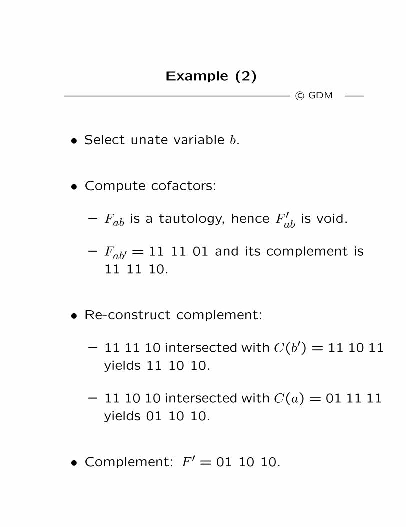
Example (2)

c© GDM

• Select unate variable b.

• Compute cofactors:

– Fab is a tautology, hence F ′ab is void.

– Fab′ = 11 11 01 and its complement is

11 11 10.

• Re-construct complement:

– 11 11 10 intersected with C(b′) = 11 10 11

yields 11 10 10.

– 11 10 10 intersected with C(a) = 01 11 11

yields 01 10 10.

• Complement: F ′ = 01 10 10.

Example (3)

c© GDM

a’ a

b’bF = TAUTa’

RECURSIVE SEARCH

COMP = φ

F = TAUTab’

COMP = φab F = c

COMP = c’

Summary

c© GDM

• Matrix oriented representation:

– Used in two-level logic minimizer.

– May be wasteful of space (sparsity).

– Good heuristics tied to this representation.

• Efficient Boolean manipulation exploits

recursion.