RELIABILITY ENGINEERING UNITASST4403

Lecture 12: DATA ANALYSIS

1

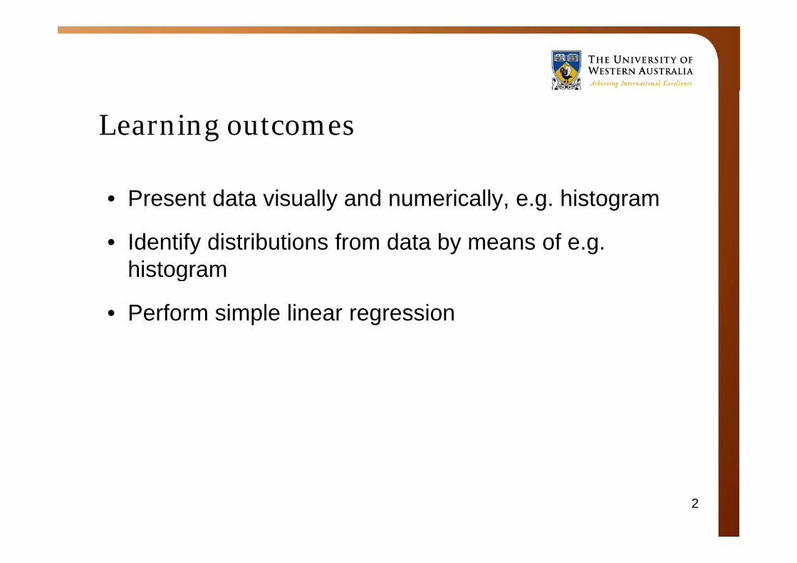
Learning outcomes

• Present data visually and numerically, e.g. histogram

• Identify distributions from data by means of e.g. histogramg

• Perform simple linear regression

2

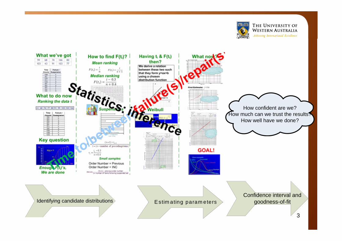
How confident are we?How much can we trust the results?

How well have we done?How well have we done?

Identifying candidate distributions Estim ating param etersConfidence interval and

goodness-of-fitde t y g ca d date d st but o s Estim ating param eters goodness of fit

3

HistogramHistogram

4

Frequency distribution

• Frequency distribution: data presented as class intervals and their corresponding frequencyintervals and their corresponding frequency

• Range: the difference between the largest and the smallest data al essmallest data values

• Number of classes (bins): Sturges' rule: select a bin size such that there are about 1 + log2n non-empty bins (n is the number of data values)

• Class midpoint: average of the class endpoints

• Relative frequency: the ratio of the frequency of the• Relative frequency: the ratio of the frequency of the class interval to the total frequency

C l ti f i t t l f th l• Cumulative frequency: running total of the classes of frequency distribution 5

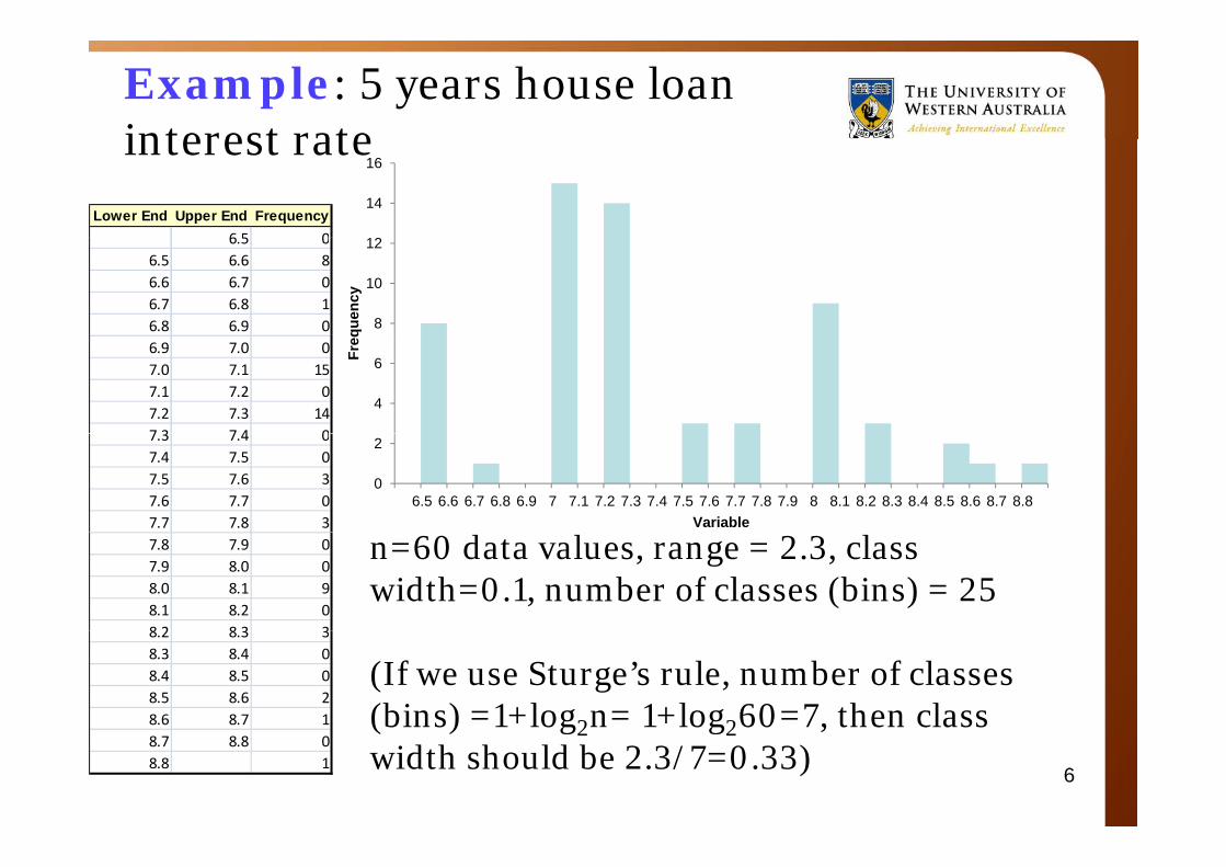
Example: 5 years house loan interest rateinterest rate

Lower End Upper End Frequency6 5 0

14

16

6.5 06.5 6.6 86.6 6.7 06.7 6.8 16.8 6.9 0 8

10

12

quen

cy6.9 7.0 07.0 7.1 157.1 7.2 07.2 7.3 147 3 7 4 0

4

6Freq

7.3 7.4 07.4 7.5 07.5 7.6 37.6 7.7 07.7 7.8 3

0

2

6.5 6.6 6.7 6.8 6.9 7 7.1 7.2 7.3 7.4 7.5 7.6 7.7 7.8 7.9 8 8.1 8.2 8.3 8.4 8.5 8.6 8.7 8.8Variable

7.8 7.9 07.9 8.0 08.0 8.1 98.1 8.2 08 2 8 3 3

n=60 data values, range = 2.3, class width=0.1, number of classes (bins) = 25

8.2 8.3 38.3 8.4 08.4 8.5 08.5 8.6 28.6 8.7 1

(If we use Sturge’s rule, number of classes (bins) =1+log2n= 1+log260=7, then class

6

8.7 8.8 08.8 1

( ) g2 g2 7,width should be 2.3/7=0.33)

Histogram

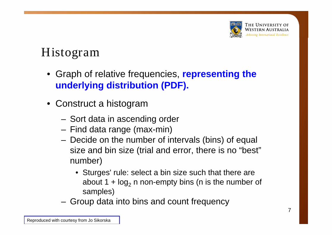
• Graph of relative frequencies, representing the underlying distribution (PDF).

• Construct a histogramSort data in ascending order– Sort data in ascending order

– Find data range (max-min)– Decide on the number of intervals (bins) of equal ( ) q

size and bin size (trial and error, there is no “best” number)

St ' l l t bi i h th t th• Sturges' rule: select a bin size such that there are about 1 + log2 n non-empty bins (n is the number of samples)

– Group data into bins and count frequency

Reproduced with courtesy from Jo Sikorska

7

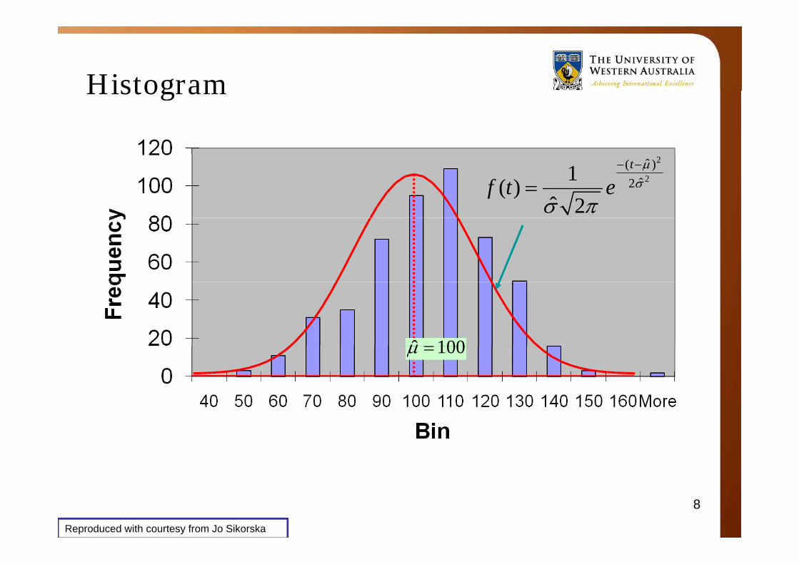
HistogramHistogram

2

2ˆ( )

ˆ21( )ˆ 2

t

f t e

100̂ 100

8

Reproduced with courtesy from Jo Sikorska

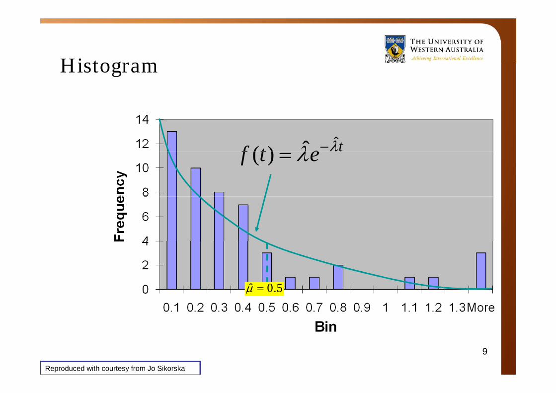
HistogramHistogram

ˆˆ( ) tf t e ( )f t e

0 5ˆ 0.5

9

Reproduced with courtesy from Jo Sikorska

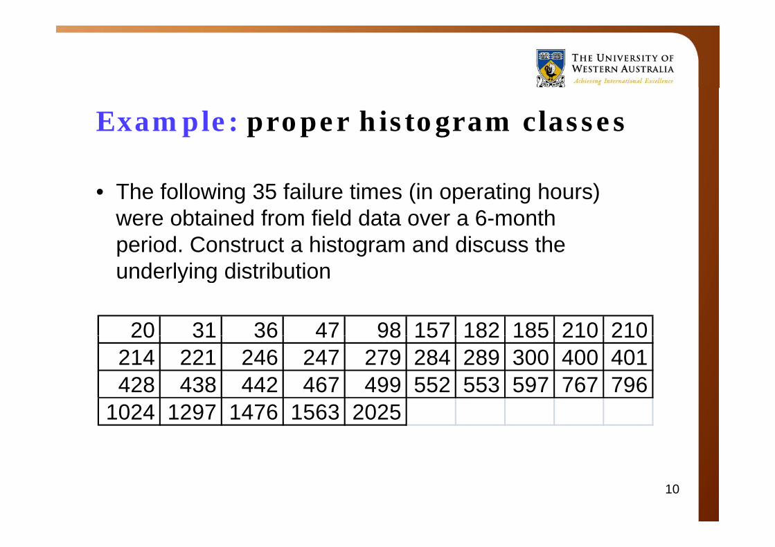
Example: proper histogram classes

• The following 35 failure times (in operating hours) bt i d f fi ld d t 6 thwere obtained from field data over a 6-month

period. Construct a histogram and discuss the underlying distributionunderlying distribution

20 31 36 47 98 157 182 185 210 21020 31 36 47 98 157 182 185 210 210214 221 246 247 279 284 289 300 400 401428 438 442 467 499 552 553 597 767 796

1024 1297 1476 1563 2025

10

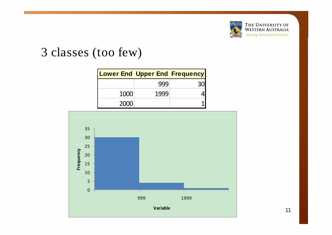
3 classes (too few)

Lower End Upper End Frequency999 30

1000 1999 42000 1

30

35

15

20

25

Freq

uency

0

5

10

999 1999

11

999 1999

Variable

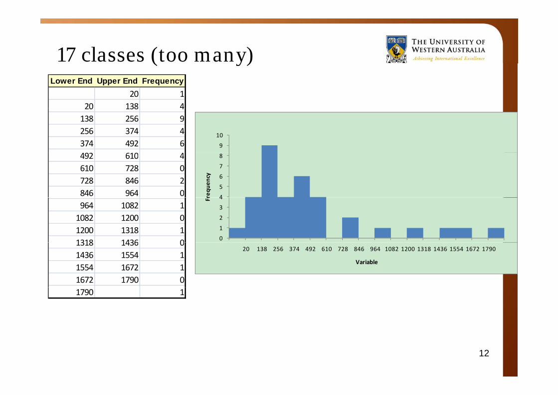
17 classes (too many)7 ( y)Lower End Upper End Frequency

20 120 138 420 138 4138 256 9256 374 4374 492 6 9

10

492 610 4610 728 0728 846 2846 964 0 4

5

6

7

8

requ

ency

964 1082 11082 1200 01200 1318 11318 1436 0 0

1

2

3

4Fr

1318 1436 01436 1554 11554 1672 11672 1790 0

20 138 256 374 492 610 728 846 964 1082 1200 1318 1436 1554 1672 1790

Variable

1790 1

12

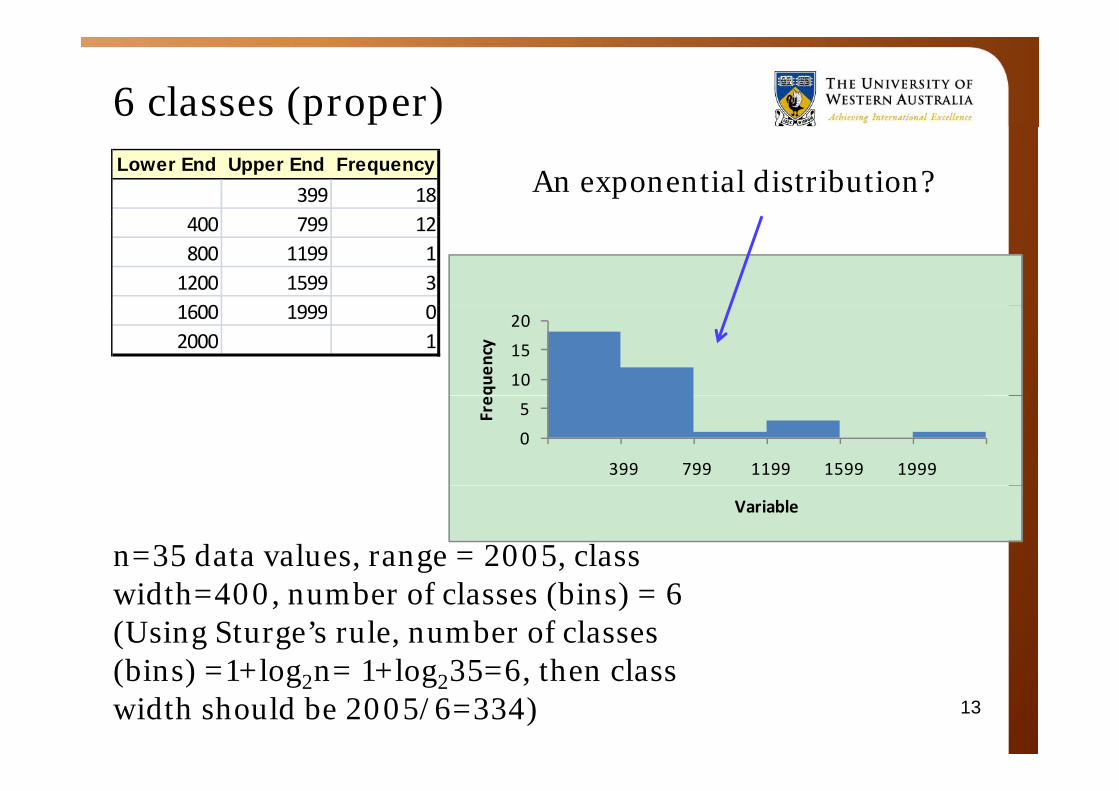
6 classes (proper)Lower End Upper End Frequency

399 18 An exponential distribution?400 799 12800 1199 11200 1599 31600 1999 01600 1999 02000 1

10

15

20

quen

cy

0

5

399 799 1199 1599 1999Fre

Variable

n=35 data values, range = 2005, class width=400, number of classes (bins) = 6(Using Sturge’s rule, number of classes (bi ) 1+l 1+l 35 6 th l

13

(bins) =1+log2n= 1+log235=6, then class width should be 2005/6=334)

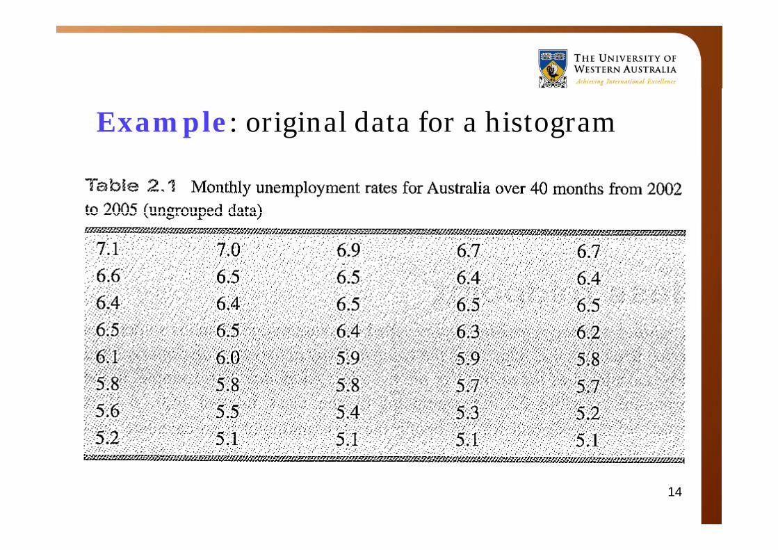
Example: original data for a histogram

14

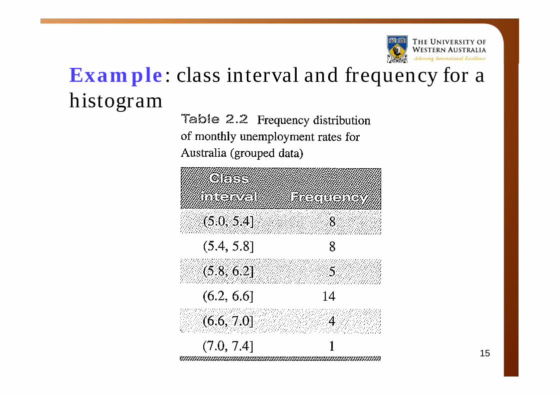
Example: class interval and frequency for a histogramg

15

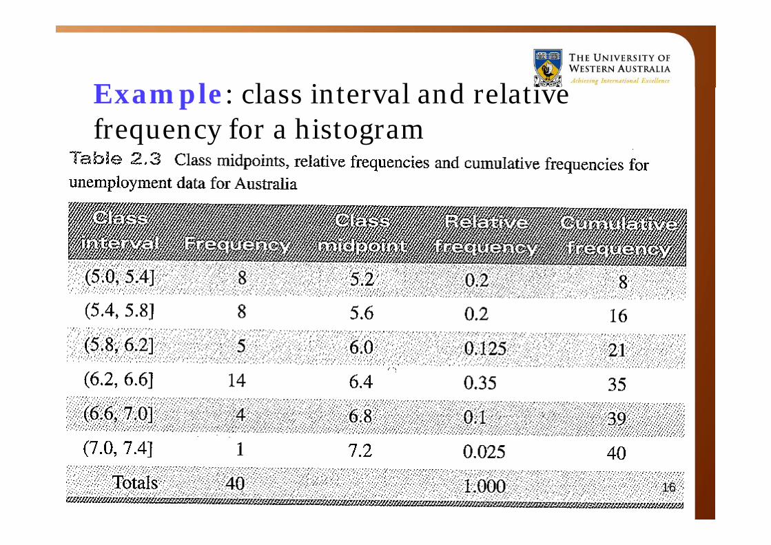
E l l i t l d l ti Example: class interval and relative frequency for a histogram

16

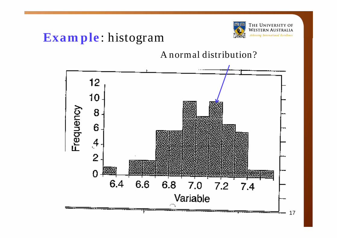
Example: histogramExample: histogramA normal distribution?

17

Simple regression

• Process of constructing a mathematical model of f ti t di t/d t i i bl bfunction to predict/determine one variable by another

• Simple regression = linear regression, two variables

• Dependent variable = the variable to be predicted, yDependent variable the variable to be predicted, y

• Independent variable (explanatory variable) =predictor x=predictor, x

• How well does it fit? Find the coefficient of l ti ( l t 1 ibl )correlation r (as close to 1 as possible)

18

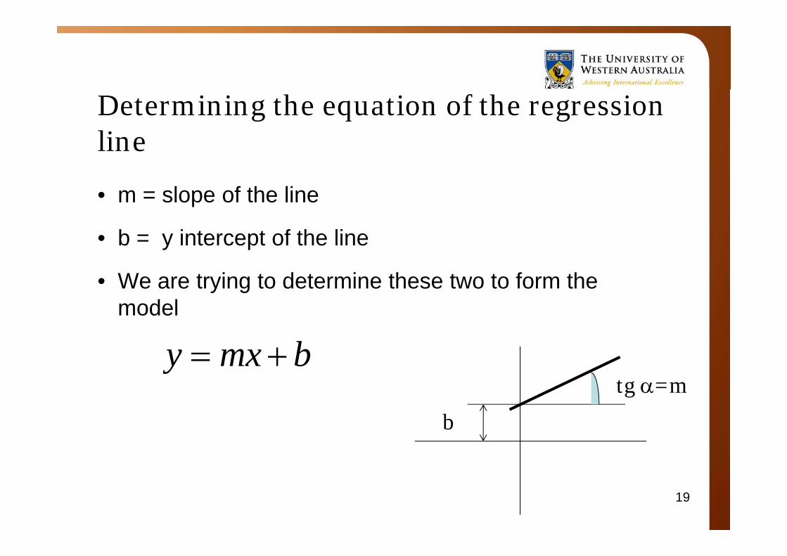
Determining the equation of the regression line

• m = slope of the line

• b = y intercept of the line

• We are trying to determine these two to form the• We are trying to determine these two to form the model

bbmxy tg =m

b

19

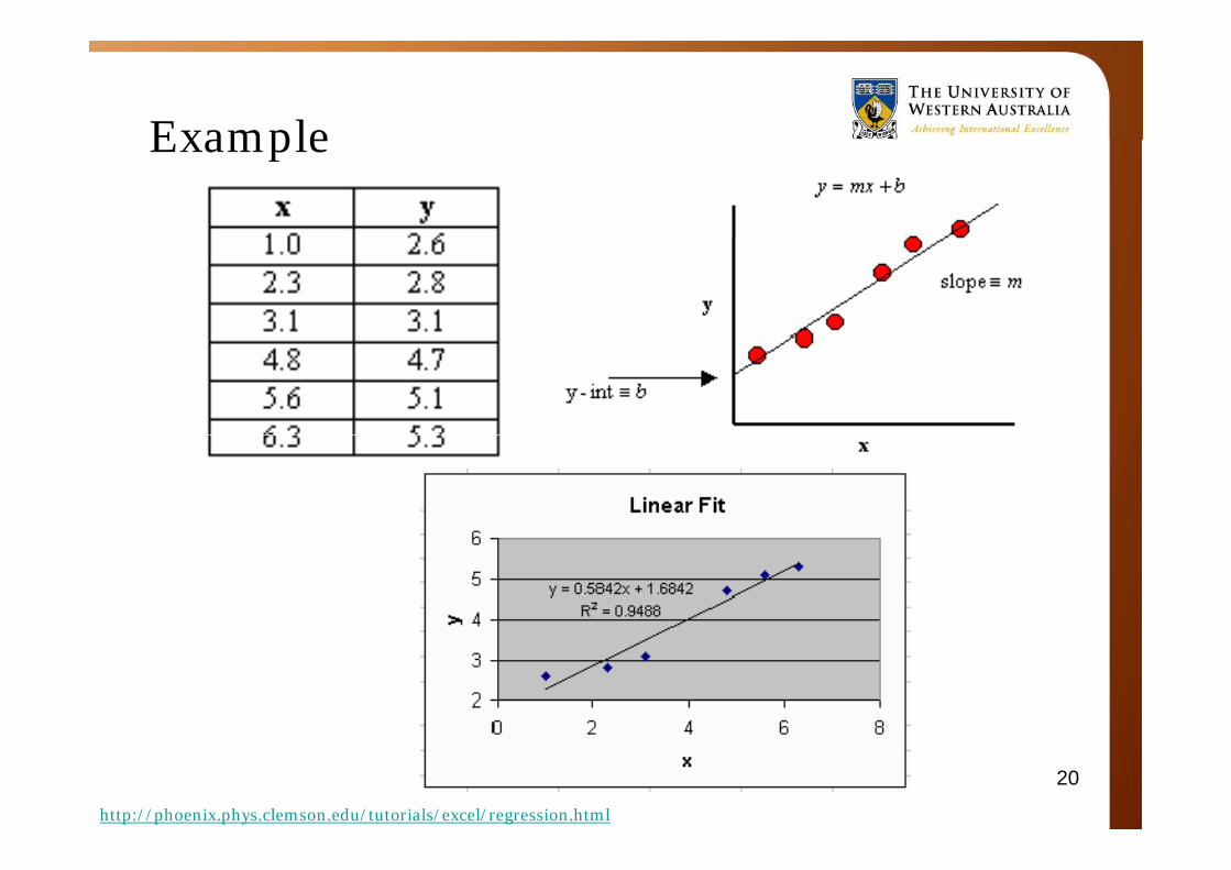
ExampleExample

20

http://phoenix.phys.clemson.edu/tutorials/excel/regression.html

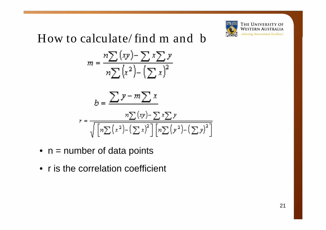
How to calculate/find m and bHow to calculate/find m and b

• n = number of data points

• r is the correlation coefficient• r is the correlation coefficient

21

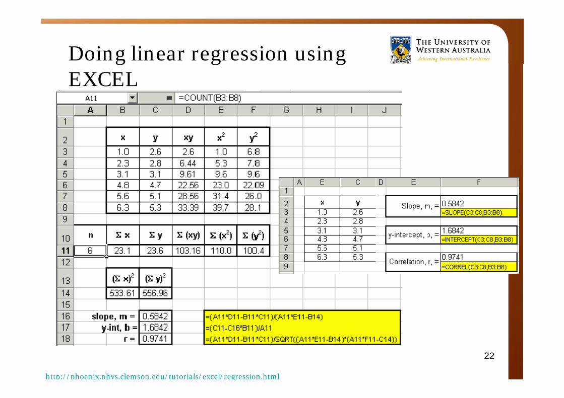
Doing linear regression using g g gEXCEL

22

http://phoenix.phys.clemson.edu/tutorials/excel/regression.html

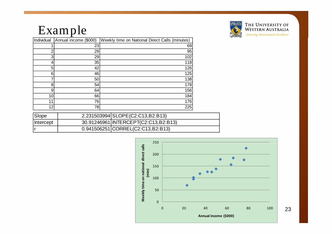
ExampleIndividual Annual income ($000) Weekly time on National Direct Calls (minutes)

1 23 692 29 953 29 1024 35 1185 42 1266 46 1257 50 1388 54 1789 64 1569 64 156

10 66 18411 76 17612 78 225

Slope 2.231503994 SLOPE(C2:C13,B2:B13)Slope 2.231503994 SLOPE(C2:C13,B2:B13)Intercept 30.91246961 INTERCEPT(C2:C13,B2:B13)r 0.941506251 CORREL(C2:C13,B2:B13)

250

150

200

50ional direct calls 

n)

50

100

eekly time on

 nat

(min

230

0 20 40 60 80 100

We

Annual income ($000)