Embed Size (px)
Citation preview

IN PARTNERSHIP WITH
DATA ANALYSIS FOR LONG-TERM MONITORINGFebruary 18, 2021

Kate Lazarus
Senior Asia ESG Advisory Lead
IFC
Introduction and Housekeeping

You will be automatically muted throughout the webinar. Please be informed that this webinarsession will be recorded.
Please do not use raise hand option. You can use the chat box on your screen to drop in yourquestions/comments directed towards a specific speaker. We will collate your comments andpresent them before speakers at appropriate times.
If you require any administrative support during the webinar, please private message Upasana Pradhan in the ZOOM chat box. We will address your concerns as best we can. ?
All the materials and presentation of this event will be shared with the participants in a few days following the webinar.
.
Today’s webinar is scheduled to last 1.30 hrs including Q&A.
HOUSEKEEPING

Agenda
19:00 - 19:10 Welcome and Housekeeping Kate Lazarus
Senior Asia ESG Advisory Lead
IFC
19:10 – 19:30 Data Analysis for Long-Term Monitoring Leeanne Alonso
Biodiversity Consultant, IFC
19:30-20:00 Data Analysis Excel Tool for monitoring fish
abundance over time (video presentation)
Jonathan Levin
PhD Candidate in Ecohydrology
University of the Witwatersrand,
South Africa
20:00 - 20:20 Q & A Moderator:
Kate Lazarus
Senior Asia ESG Advisory Lead
IFC
20:20-20:30 Closing Remarks Babacar Faye
Resident Representative, IFC,
Nepal

Data Analysis
for Long-term Monitoring
Presenters:
Leeanne Alonso
Biodiversity Consultant, IFC
Jonathan Levin
PhD Candidate in Ecohydrology
University of the Witwatersrand, South Africa

Why the Tool is needed- slides from Deep
Talk Outline
Why Biodiversity Monitoring
Sampling Design and Field
Methods
Data Analysis and Metrics
Data Analysis Excel Tool
for monitoring fish
abundance over time
Trishuli River Basin

Why Biodiversity Monitoring
6

What is Biodiversity Monitoring?
• Biodiversity monitoring is the process of determining status and tracking changes in living organisms and the
ecological complexes of which they are a part.
• Biodiversity monitoring is important because it provides a basis for evaluating the integrity of
ecosystems, their responses to disturbances, and the success of actions taken to conserve or
recover biodiversity.
• Research addresses questions and tests hypotheses about how these ecosystems function and change and
how they interact with stressors.
• Ecological research provides the context for interpreting these monitoring results. Policy and management
needs guide the development of monitoring.
7
https://biodivcanada.chm-cbd.net/ecosystem-status-trends-2010/biodiversity-monitoring-research-information-management-and-
reporting#:~:text=Biodiversity%20monitoring%20is%20the%20process%20of%20determining%20status,of%20actions%20taken%20to%20conserve%20or%20recover%20
biodiversity.

ESIA and IFC PS6 General Process for Hydropower Project
1. Hydropower Project is proposed
2. ESIA is required per EIA Manual for Hydropower (2018) for Government of Nepal and per GIIP for IFC
3. Baseline biodiversity data collection for ESIA
4. Impact Assessment using the baseline biodiversity data collected (literature and field)
5. Mitigation is developed per the Mitigation Hierarchy to avoid, minimize and, if needed, offset impacts
6. IFC’s PS6 requires project to achieve and demonstrate No Net Loss of Biodiversity (NNL) for Natural Habitat
Values and Net Gain (NG) for Critical Habitat Values
7. Monitoring program is developed to demonstrate that the mitigation measures committed in the
ESIA are successful and that NNL/NG is achieved for government and lender compliance
8

ESIA Baseline
1. Provides the Baseline on biodiversity and ecosystem values used for:
• Impact Assessment
• Mitigation Actions
Thus Baseline sampling for an ESIA should utilize all possible field sampling methods, at as many
sites, and as frequently as possible to maximize the data available to make these decisions.
The More Data the Better!
2. Often provides the Pre-construction Baseline for the Long-term Monitoring program
• Extremely Important- Will be used to compare to all future years for Monitoring
• Think Ahead- Need to include the sampling protocol for Monitoring because Monitoring
requires standardized, repeated data collection in order to make valid comparisons over
time- using same field methods, same sites, same dates, same researchers, same data
collection and analysis
• Baseline for Monitoring must be collected as early as possible - at least 1 year before
construction and ideally for several years before construction
*This is lacking in most monitoring programs
9

What is No Net Loss (NNL) and Net Gain (NG)?
How will we know when it is achieved?
IFC Performance Standard 6 (2012)
Paragraph 15, Footnote 9:
No net loss is defined as the point at which project-related impacts on biodiversity are balanced by measures
taken to avoid and minimize the project’s impacts, to undertake on-site restoration and finally to offset
significant residual impacts, if any, on an appropriate geographic scale (e.g., local, landscape-level, national,
regional).
Paragraph 18, Footnote 15:
Net gains are additional conservation outcomes that can be achieved for the biodiversity values for which the
critical habitat was designated. Net gains may be achieved through the development of a biodiversity offset
and/or, in instances where the client could meet the requirements of paragraph 17 of this Performance
Standard without a biodiversity offset, the client should achieve net gains through the implementation of
programs that could be implemented in situ (on-the-ground) to enhance habitat, and protect and conserve
biodiversity.
https://www.ifc.org/wps/wcm/connect/topics_ext_content/ifc_external_corporate_site/sustainability-at-ifc/policies-standards/performance-
standards/ps6
10

IFC PS6 Guidance Note (2012, Updated 2019)
GN43 A defensible rationale for how no net loss will be achieved should be provided. A variety of methods exist to calculate losses and
gains of the quantity and quality of identified biodiversity values and to assess the likelihood of success of proposed mitigation and management
actions. While appropriate methods and metrics will vary from site to site, these should be evidence-based, utilizing quantitative and semi-
quantitative methods as inputs to an expert-led process. The level of confidence in the results of the analysis should be commensurate with the
risks and impacts that the project poses to the natural habitat.
GN51. Long-term biodiversity monitoring may be required to validate the accuracy of predicted impacts and risks to biodiversity
values posed by the project, and the predicted effectiveness of biodiversity management actions. The monitoring and evaluation
program should include the following: (i) baseline, measures of the status of biodiversity values prior to the project’s impacts; (ii) process,
monitoring of the implementation of mitigation measures and management controls; and (iii) outcomes, monitoring of the status of biodiversity
values during the life of the project, compared to the baseline. In addition, clients should consider controls, monitoring in comparable areas
where project impacts are not occurring to detect effects unrelated to project impacts. The client is expected to develop a practical set of
indicators (metrics) for the biodiversity values requiring mitigation and management. Indicators and sampling design should be
selected on the basis of utility, that is, their ability to inform decisions about mitigation and management, and effectiveness, their
ability to measure effects with adequate statistical power given the estimated ranges of natural variability for each biodiversity value.
Proxy indicators for some biodiversity values may be necessary to satisfy these criteria.
GN52. Specific thresholds should be set for monitoring results that will trigger a need to adapt the management plan(s) to address any
deficiencies in performance. The results of the monitoring program should be reviewed regularly. If they indicate that the actions specified in the
management plan(s) are not being implemented as planned, the reasons for failure need to be identified (for example, insufficient staff,
insufficient resources, unrealistic timeline, etc.) and rectified. If outcome monitoring results indicate that project impacts to biodiversity values
were underestimated or that the benefits to biodiversity from management actions including offsets were overestimated, the impact assessment
and management plans should be updated.
11

IFC PS6 Guidance Note (2012, Updated 2019)
GN90. In areas of critical habitat, the client will be expected to demonstrate net gains in biodiversity values
for which the critical habitat was designated, as stated in paragraph 18 of Performance Standard 6. Net gains
are defined in footnote 15 of Performance Standard 6 and could be considered “no net loss plus;” therefore,
the requirements defined for critical habitat build upon and expand those defined for natural habitat.
Net gains may be achieved through the biodiversity offset. As described in footnote 15 of Performance
Standard 6, net gains of biodiversity values must involve measurable, additional conservation outcomes. Such
gains must be demonstrated on an appropriate geographic scale (e.g., local, landscape-level, national, regional)
as determined by external experts. In instances where a biodiversity offset is not part of the client’s mitigation
strategy (i.e., there are no significant residual impacts), net gains may be obtained by supporting additional
opportunities to conserve the critical habitat values in question. In these cases, qualitative evidence and expert
opinion may be sufficient to validate a net gain.
12

Pressure-State-Response Monitoring Approach
There are many approaches to long-term monitoring for biodiversity that can be used.
One good approach is the Pressure-State-Response Model in which the program monitors:
Pressure Indicators – Indicators of the stressors or impacts (e.g. minimum river flow rate in dry season, #days
dry river, #illegal fishing nets, #sand mining operations)
State Indicators – Indicators of the current state/condition of the target biodiversity values (e.g. #fish
individuals/hour, macroinvertebrate indices, area of riverine habitat)
Response Indicators – Indicators of the mitigation actions implemented to avoid or reduce impacts on
biodiversity (e.g. release of EFlows, fish ladder operation, #patrols for illegal fishing, km of river enhanced)
13

Sampling Design and Field Methods
14

Sampling Design for Hydropower Project
A Monitoring Program should include sampling in three River Units:
1. Upstream of Hydropower Project, including reservoir area
2. Diversion reach
3. Downstream of Power House (especially if a peaking Project)
Within each River Unit, sampling sites should include:
• Main Stem
• Large Tributaries
• Small Tributaries
• River Tributaries
15

Common sampling design and data presentation for project monitoring
Not Adequate
• Set of sampling sites across the entire project area, rather than in the 3 target River Units
• Small number of sampling sites (<5)
• Combining the data for total # of species, or total # individuals across all sites (and all methods)
16
Plotting one number per site is not representative Need to understand the natural variation

Need Multiple Samples (Replicates) to capture Natural Variation
Due to the high variation in natural ecosystems, it is important to have Multiple Replicates per River Unit
(Upstream, Diversion Reach, Downstream of Power House)
• Replicates can be Spatial – multiple sites
• Replicates can be Temporal – multiple dates
• Due to time and cost constraints, replicates are usually done spatially
• Statistical analyses to compare data over time require at least 5 replicates per sampling period (e.g. season)
(Again, the more sampling sites the better!)
Trishuli Assessment Tool recommends 6 sampling sites in each of the 3 River Units (18 sampling sites)
18

Example of Temporal Replicates
Migrating Raptors counts, September 2020 USA
19

HPP Dam
HPP Powerhouse
River Unit 1: Upstream of Dam
(6 sampling sites)
River Unit 2: Diversion Reach
Between dam and powerhouse
(6 sampling sites)
River Unit 3: Downstream of Powerhouse
(6 sampling sites)
Example Monitoring Sampling Design

At each sampling site, apply the Trishuli Assessment Tool Field Methods21

Sampling Effort for each Field Method - Standardized 22
Method Effort Units Number of units Approx. Sampling/
Total Time*RECORD THE TIME SPENT SAMPLING
Personnel
Electrofishing Time sampling with
current on (minutes)
20 min US/20 min DS
(40 minutes total/site)
40 min/120 min 3 people
Cast Net Cast Net Throws
Time for 25 throws
(mins)
12 US/1 MP/12 DS
(25 total/site)
60 min/120 min 2 people
Dip Net Dip Net Emersions 10 samples/site 30 min/60 min 1 person
Underwater Video Camera sets 5 minute recording/set
6 sets US / 6 sets DS
(12 sets/site)
60 min/90 min 1 person
eDNA 2 L water samples 5 samples+1 control/site
(6 samples/site)
60 min/180 min 2-4 people
Macroinvertebrate
sampling
Net subsamples 20 total over different
substrate types
60 min/150 min 2-3 people
Periphyton sampling Rock Scraped 5 per site 15 min/30 min 2-3 people

Metrics and Data Analysis
23

Long-term Monitoring Questions and Metrics
Questions
1. How has the number of individuals of target species changed over time?
2. How has the number of species changed over time?
3. How has the distribution of species changed over time?
4. How has the composition of species changed over time?
Monitoring analysis requires specific Metrics to quantitatively compare over time
1. CPUE = Catch (# individuals) Per Unit Effort (hours) per site per season per year
2. SPUE = Species (# species) Per Unit Effort (hours)
3. Habitat area (m2) (e.g. riffle habitat)
4. #juvenile fish/10 dip nets
5. Macroinvertebrate analysis has specific indices and metrics (see Macroinvertebrate webinar)
24

Quantitative Metrics for Long-term Monitoring with the Trishuli Assessment Tool
Target Indicator Metric
Overall Aquatic Biodiversity Composition Species names
Species Richness (# species) # species / hour (SPUE)
Abundance of target species # individuals / hour (CPUE)
Snow Trout adults and juveniles (Schizothorax richardsonii)
Abundance # individuals / hour (CPUE)
Golden Mahaseer adults and juveniles (Tor putitora)
Abundance # individuals / hour (CPUE)
Macroinvertebrates/Periphyton Richness and abundance of key taxa EPT Index
Functional Feeding Groups Ratio of groups
25

Common Snow Trout, Schizothorax richardsonii
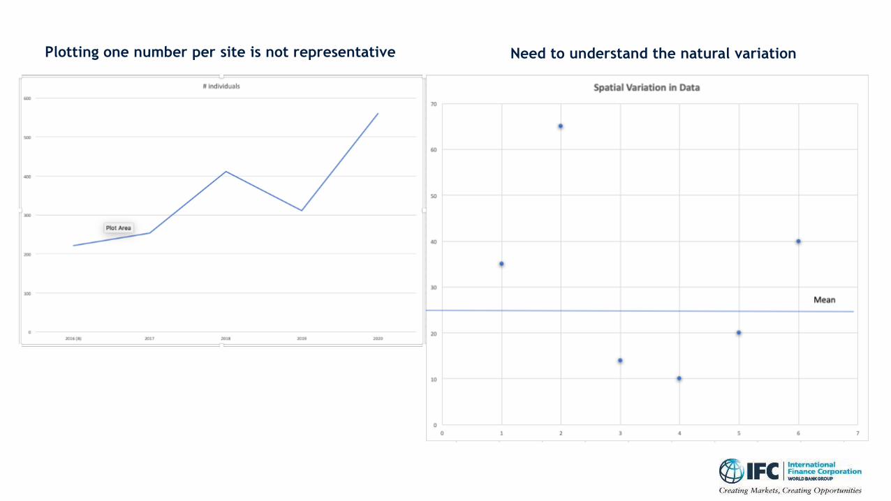
Data Collection
Sample Data from the Tadi Khola, February 2020
Metric Electrofishing Cast Nets Dip Nets
Total # fish individuals (N) 106 20 30
Total Effort (minutes) 32 57 20
Total Effort (hours) 0.53 0.95 0.33
CPUE (# individuals/hour) 199 21.1 90
Species Richness - Total # fish species (S) 15 4 1
SPUE (# species/hour) 28 4.2 3
27

Monitoring Comparisons: Compare Like with Like
• Control for other variables that may cause differences/changes such as season, location, time of day,
researcher, climatic events, other disturbances, etc.
• Comparisons made for each River Unit separately (6 sampling points/unit)
• Upstream Baseline compared to Upstream Monitoring Year 1, Year 2, etc.
• Diversion Reach Baseline compared to Diversion Reach Monitoring Year 1, Year 2, etc.
• Downstream of Powerhouse Baseline compared to Downstream Monitoring Year 1, Year 2, etc.
• Baseline Year (pre-construction) compared to Monitoring Years (during and post-construction)
• Same Season compared to Same Season
• February compared to February
• October compared to October
28

Data Analysis Excel Tool
for monitoring fish abundance over timeTool is based in Excel for ease of use, linked with statistical program ‘R’
Tool was developed by:
• Jonathan Levin, University of Witswatersrand, Johannesburg, South Africa
• Gina Walsh, Aquatic Biologist, Consultant and The Biodiversity Consultancy
• Claire Fletcher, The Biodiversity Consultancy
• Emma Hume, The Biodiversity Consultancy
Objective of the Tool:
To provide a simple user-friendly data analysis tool to compare monitoring data over time to:
• Track changes in indicator/metric
• Assess mitigation success
• Demonstrate NNL or NG to meet lender’s requirements
• This version was designed for snow trout in Trishuli River, but can be modified for other
species and locations, as well as other metrics
The Tool is still in development/refinement. We welcome comments and suggestions.
We can schedule another session to discuss the details if people are interested.
29

Step 1: Enter Field Data into Excel Spreadsheet
30
Sampling Site Sampling
Method
# fish Time (Minutes)
Upstream 1 Electrofishing
Cast Nets
Dip Nets
Video (Camera)
Seine Nets
Upstream 2 Electrofishing
Cast Nets
Dip Nets
Video (Camera)
Seine Nets
…..

Step 2: Excel Tool calculates standardized CPUE for all field methods combined
Step 3: Compare Mean Standardized CPUE between Baseline and Monitoring Year(s)
31
≥
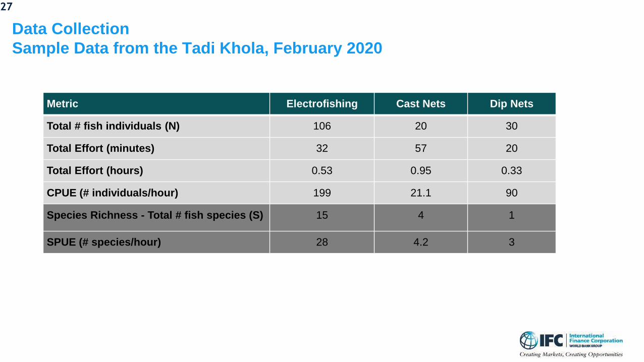
Step 4: Visualize the Data Comparison with BoxPlot
32

Step 5: Visual Trends Analysis and Thresholds for NNL and Net Gain
Numerical Thresholds and Adaptive Management
33

Data Analysis Excel Tool
for monitoring fish abundance over time
(video presentation)
Presenter:
Jonathan Levin
PhD Candidate in Ecohydrology
University of the Witwatersrand,
South Africa

Moderator:
Ms. Kate Lazarus
Senior Asia ESG Lead
IFC
Q & A Session

Next Steps
Trishuli Assessment Tool Kit
• Manual
• Recordings of February Webinars
• Powerpoints from February Webinars
• In-person Training Courses
Develop local capacity for the Trishuli Assessment Tool
Promote use of the Trishuli Assessment Tool for ESIAs
• NEA
• Private Hydropower Developers
• Everyone!
Link with the Freshwater Ecosystem Assessment Handbook
• Companion handbook to the Hydropower Environmental Impact
Assessment Manual (MoFE)
• Forthcoming from ICIMOD and Forest Research Training Centre (FRTC)
• Prepared by Deep Shah and Ram Devi Tachamo Shah
• Webinar on May 11
http://mofe.gov.np/downloadfile/Hydropower%20Env
ironmental%20Impact%20Assessment%20Manual_153
7854204.pdf
Next up in the IFC Webinar Series
Coming up in March:
❖ March 16: Novel approaches to tracking fish movements
❖ March 23: Re-thinking Hatcheries: A Review of costs and benefits
by Julie Claussen and David Phillip, Fisheries Conservation Foundation
37

Closing Remarks
Babacar Faye
Resident Representative
IFC, Nepal

Thank you !