Data Analysis in Geophysics �ESCI 7205

�Bob Smalley�

Room 103 in 3892 (long building), x-4929 �

Tu/Th - 13:00-14:30 �CERI MAC (or STUDENT) LAB

Lab – 9, 09/24/13

Unary Operations Module

The commands in this module perform some arithmetic operation on each data point of the

signals in memory.

add!sub!mul!div!sqr!sqrt!

abs!log,log10!exp,exp10!

int !dif!

Read in some data – do some processing

SAC> read ./ccm_solomon*bh?!…!SAC> p1!

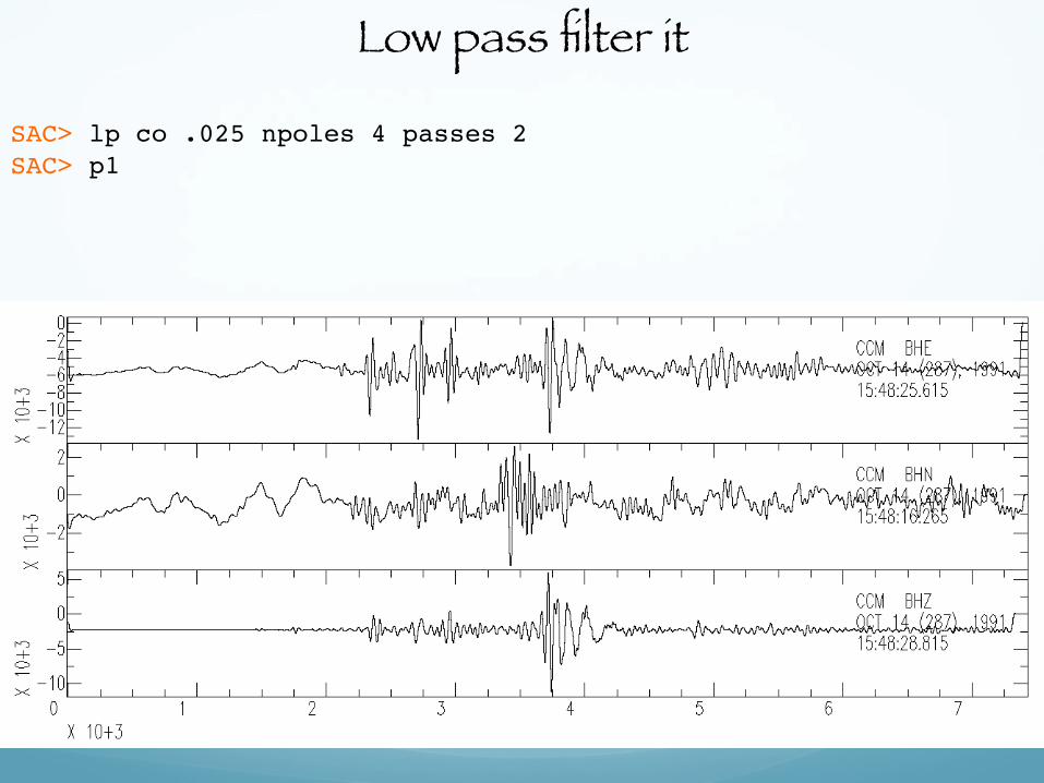
Low pass filter it

SAC> lp co .025 npoles 4 passes 2!SAC> p1!

High pass filter it

SAC> r SAC> hp co 1 npoles 4!SAC> p1!

Spectral analysis – Fourier transform SAC> read ccm_solomon_*z!SAC> fft!SAC> psp!Waiting!SAC> !

Rotate seismograms!SAC> read *TUL1*SAC!2010.058.06.42.30.9750.TA.TUL1..BHN.R.SAC … !SAC> p1!SAC> synch!SAC> w TUL1.BHN TUL1.BHE TUL1.BHZ!SAC> cut 0 1800!SAC> r TUL1.BHN TUL1.BHE!SAC> rotate!SAC> lh! FILE: TUL1.BHE - 1! --------------!...!

! ! STLA = 3.591040e+01! STLO = -9.579190e+01! STEL = 2.560000e+02! STDP = 0.000000e+00! EVLA = -3.612200e+01! EVLO = -7.289800e+01! EVDP = 2.290000e+04!

! ! DIST = 8.319518e+03! AZ = 3.408942e+02! BAZ = 1.609469e+02! GCARC = 7.476556e+01!...!

SAC> read *BHZ*SAC!2010.058.06.41.47.2750.TA.035Z..BHZ.R.SAC!...!SAC> qdp off!SAC> p1!SAC> sss! Signal Stacking Subprocess.!SAC/SSS> prs!

SAC> r ./2010.058.06.41.47.2750.TA.035Z..BHZ.R.SAC …!SAC> p1!SAC> rmean!SAC> taper!SAC> correlate!SAC> p1!

Signal Correction Module

These commands let you perform certain signal correction operations.

-  rmean: removes the mean from data.

-  rtrend: removes linear trend (and mean) from data.

- rglitches: removes glitches and timing marks.

-  taper: applies a symmetric taper to each end of the data and SMOOTH applies an arithmetic smoothing

algorithm.

-  linefit: computes the best straight line fit to the data in memory and writes the results to header blackboard

variables.

- reverse: reverses the order of data points.

Integration – to change from acceleration to velocity, and velocity to displacement.

SAC> r ccm_india_.bhz!SAC> qdp off!SAC> plot!

Integrate it (original data was vel, integrate to disp).

SAC> int!SAC> p!

OOPS!

What is the problem?

(do you agree that there is a problem?!)

Integral of constant is a straight sloping line.

The seismic data has a (small) DC offset (a constant).

So remove the mean.

Try again.

SAC> r!SAC> rmean!SAC> int!SAC> p!!

OOPS again!

Is this an improvement? Are we getting any better?

What’s the problem now?

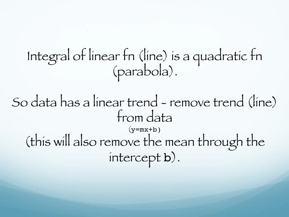
Integral of linear fn (line) is a quadratic fn (parabola).

So data has a linear trend - remove trend (line)

from data (y=mx+b)!

(this will also remove the mean through the intercept b).

Remove trend (line) with rtrend.!SAC> r!SAC> rtrend! Slope and standard deviation are: -0.038705 0.0037565! Intercept and standard deviation are: -2365.1 15.788! Data standard deviation is: 3010.9! Data correlation coefficient is: 0.026988!SAC> int!SAC> p!

Removing the line will also remove the mean if it is not zero.

So don’t really need to do the rmean first.

There is still some “drift”, but this seismogram might be useful for displacement analysis.

SAC> r!SAC> rtrend! Slope and standard deviation are: -0.038705 0.0037565! Intercept and standard deviation are: -2365.1 15.788! Data standard deviation is: 3010.9! Data correlation coefficient is: 0.026988!SAC> int!SAC> r more!SAC> p1!

SAC> r more SAC> p1

displacement

velocity

Big problems with "baseline" drift when trying to integrate acceleration up to displacement to when

trying to obtain/estimate co-seismic static displacement.

Boore, 2001

Differentiation - default is 2 point difference y=(x1-x0)/delta.�sac> funcgen impulse delta 0.01 npts 100 sac> dif !sac> p!

Differentiate velocity to acceleration.

SAC> r!SAC> dif!SAC> p!

Binary Operations Module

These commands perform operations on pairs of data files.

-  merge: merges (concatenates) a set of files to the data in memory.

Binary Operations Module

-  addf: Adds a set of data files to data in memory.

!READ FILE1 FILE2!ADDF FILE3 FILE4!!READ FILE1 FILE2 FILE3!ADDF FILE4!

-  subf: subtracts a set of data files from the ones in memory.

-  mulf: multiplies the data in memory by a set of data files.

-  divf: divides the data in memory by a set of files.

- binoperr: controls errors that can occur during these binary operations. Can use to override the requirement

for the same number of points and/or the same sampling interval.

sac> funcgen impulse delta 0.01 npts 100 sac> w impulse1.sac sac> div 2 ! !sac> w impulse2.sac sac> r impulse1.sac sac> addf impulse2.sac

Notice you have to write intermediate stuff out to disk.

sac> funcgen sine 10 90 delta 0.01 npts 100 sac> p sac> taper !

More

-  stretch: upsamples data, including an optional interpolating FIR filter.

-  decimate: downsamples data, including an optional anti-aliasing FIR filter.

- interpolate: interpolate evenly or unevenly spaced data to a new sampling interval using the interpolate

command.

More

-  quantize: converts continuous data into its quantized equivalent.

-  rotate: pairs of data components through a specified

angle.

- rq: removes the seismic Q factor from spectral data.

sac> r II.AAK.00.BHN.Q.SAC II.AAK.00.BHE.Q.SAC sac> p1 sac> rotate to gcp normal !

Radial : SV

Transverse : SH

baz = 146º

Spectral Analysis Module

There is a set of Infinite Impulse Response (IIR) filters.

lowpass (lp) passes signal below a high corner cutoff.

highpass (hp) passes signal above a low corner cutoff).

bandpass (bp) pass signal within the low and high corner cutoffs.

bandrej (br) band reject filter does the opposite of a bandpass.

These recursive digital filters are all based upon classical analog designs

Butterworth: a good choice for most applications, since it has a fairly sharp transition

from pass band to stop band, and its group delay (phase) response is moderate. This is the

default.

Bessel: best for those applications which require linear phase without two-pass filtering.

It's amplitude response is not very good however.

Chebyshev type I & Chebyshev type II:

for situations which require very rapid transitions from pass band to stop band.

Does horrible things to the phase.

The Butterworth filter rolls off more slowly around the cutoff frequency than the Chebyshev

filter or the Elliptic filter, but without ripple.

The Butterworth filter is relatively nice with the phase.

The Butterworth and Bessel are the easiest to set up�BANDPASS {BUTTER|BESSEL|C1|C2},{CORNERS v1 v2},{NPOLES n},{PASSES n},{TRANBW v},{ATTEN v} sac> funcgen seismogram sac> rmean sac> taper sac> bp butter co 1 3 �

using default values �passes (p) 1 �num poles (n) 2

sac> hp butter co .2 sac> xlim t1 -120 800 !

sac> funcgen seismogram sac> bp butter co 1 3 sac> rmean sac> taper sac> bp bessel co 1 3 n 1 p 2 !

Other filters

Finite Impulse Response filter (FIR).

Adaptive Wiener filter. (It tailors itself to be the “best possible filter” for a given dataset.).

Two specialized filters (BENIOFF & KHRONHITE).

(lowpass filter is a digital approximation of an analog filter which was a cascade of two

fourth-order Butterworth lowpass filters. This lowpass filter has been used with a corner frequency of 0.1 Hz to enhance measurements of the amplitudes of the fundamental

mode Rayleigh wave (Rg) at regional distances.)

Instrument Correction Module.

This module currently contains only one command,

transfer.

transfer: performs a deconvolution to remove one instrument response followed a convolution

to apply another instrument response.

>40 predefined instrument responses available.

A general instrument response can also be specified in terms of its poles and zeros.

sac> funcgen seismogram sac> transfer to wa

Usually you would remove the known instrument response using ‘transfer from XXX’.

Why would you want to remove the instrument response and apply the response for a Wood-

Anderson torsion seismometer?

Let’s say you’ve downloaded some data from IRIS, unpacked the seed volume using rdseed,

and extracted the response files. (RESP.NET.STA.LOC.CHAN) �

�

transfer can read seed response files (evalresp) and transform velocity to

displacement (none).

sac> r BJT* sac> rtrend sac> rmean sac> transfer from evalresp to none

Spectral Analysis Module (SAM): Spectral/Fourier Transform analysis.

You can do a discrete Fourier transform

fft!

and an inverse Fourier transform

ifft

You can also compute the amplitude and unwrapped phase of a signal (“unwrap”). This

is an implementation of the algorithm due to Tribolet.

The fft and

unwrap

commands produce spectral data in memory.

You can plot this spectral data

plotsp

You can write it to disk as

writesp

and

read in back in again

readsp

You have to know the data/file is spectral data. SAC will not figure it out.

You can also perform

- integration with

divomega!

and

- differentiation with

mulomega

directly in the frequency domain.

sac> funcgen seismogram sac> fft sac> plotsp!

Plots amplitude

Then the phase after a <CR>

SPECTROGRAM!(DEFAULT VALUES: SPECTROGRAM WINDOW 2, SLICE 1, METHOD MEM, ORDER

100, NOSCALING, YMIN 0, YMAX FNYQUIST, COLOR)

sac> funcgen seismogramsac> spectrogram ymin 0 ymax 20Window size: 200 Overlap: 100 FFT size: 512 !Spectrogram dimensions are 512 by 9 .!!

SAC> help spectrogram!!SAC Command Reference Manual SPECTROGRAM!!SUMMARY:!Calculate a spectrogram using all of the data in memory.!!SYNTAX:!SPECTROGRAM options!where options are one or more of the following:! !WINDOW v!SLICE v!ORDER n!CBAR {ON|OFF}!{SQRT|NLOG|LOG10|NOSCALING}!YMIN v!YMAX v!METHOD {PDS|MEM|MLM}!{COLOR|GRAY}!PRINT {pname}! !INPUT:! WINDOW v : Set the sliding data window length in seconds to v. This! window length determines the size of the fft. !! SLICE v : Set the data slice interval in seconds to v. A single! spectrogram line is produced for each slice interval. !! ORDER n : Specifies the number of points in the autocorrelation! function used to compute the spectral estimate. !! CBAR {ON|OFF} : Turn reference color bar on or off. !! {SQRT|NLOG|LOG10|NOSCALING} : Specify natural log, log base 10, or! square root scaling of amplitudes. !! YMIN v : Specifies the minimum frequency to plot. !! YMAX v : Specifies the maximum frequency to plot. !! METHOD {PDS|MEM|MLM} : Specifies the type of spectral estimator used.! MLM stands for maximum likelihood and MEM stands for maximum! entropy spectral estimators, respectively. See description and! references below. !! {COLOR|GRAY} : Specifies a color or grayscale image.!! PRINT {pname} : Prints the resulting plot to the printer named in! pname, or to the default printer if pname is not used. (This! makes use of the SGF capability.)!!DEFAULT VALUES:!SPECTROGRAM WINDOW 2 SLICE 1 METHOD MEM ORDER 100 NOSCALING YMIN 0 YMAX!FNYQUIST COLOR!!DESCRIPTION: …!