Embed Size (px)
Citation preview

DATA ANALYSIS
Module Code: CA660
Lecture Block 2
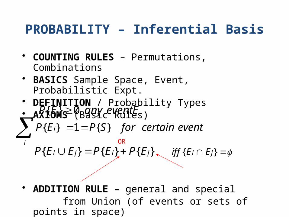
PROBABILITY – Inferential Basis
• COUNTING RULES – Permutations, Combinations• BASICS Sample Space, Event, Probabilistic Expt.• DEFINITION / Probability Types • AXIOMS (Basic Rules)
• ADDITION RULE – general and special from Union (of events or sets of points in space)
}{}{}{}{ jijiji EEiffEPEPEEP
EeventanyEP 0}{ eventcertainforSPEP
i
i }{1}{ OR
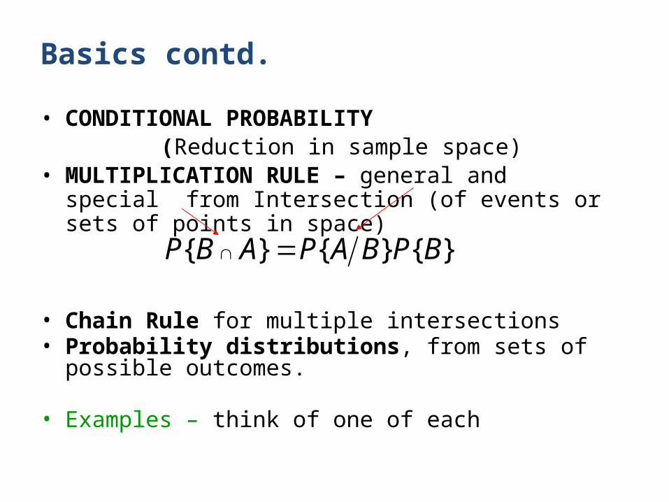
Basics contd. • CONDITIONAL PROBABILITY (Reduction in sample space)• MULTIPLICATION RULE – general and special from
Intersection (of events or sets of points in space)
• Chain Rule for multiple intersections• Probability distributions, from sets of possible outcomes.
• Examples – think of one of each
}{}{}{ BPBAPABP
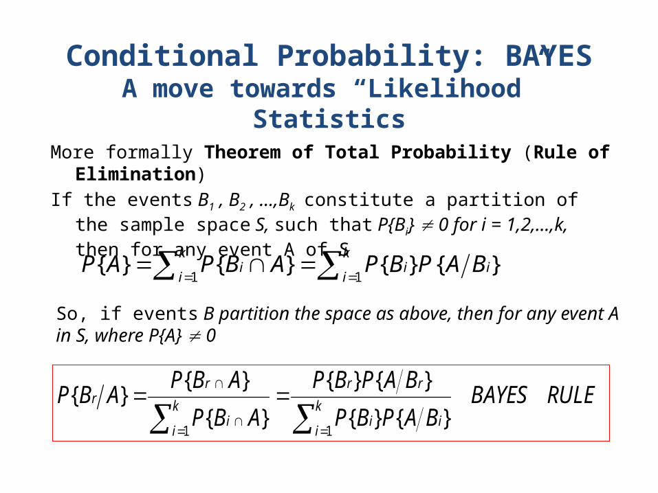
Conditional Probability: BAYESA move towards “Likelihood” Statistics
More formally Theorem of Total Probability (Rule of Elimination)If the events B1 , B2 , …,Bk constitute a partition of the sample space S, such
that P{Bi} 0 for i = 1,2,…,k, then for any event A of S
k
iii
k
ii BAPBPABPAP
11}{}{}{}{
So, if events B partition the space as above, then for any event A in S, where P{A} 0
RULEBAYESBAPBP
BAPBP
ABP
ABPABP k
iii
rr
k
ii
rr
11}{}{
}{}{
}{
}{}{
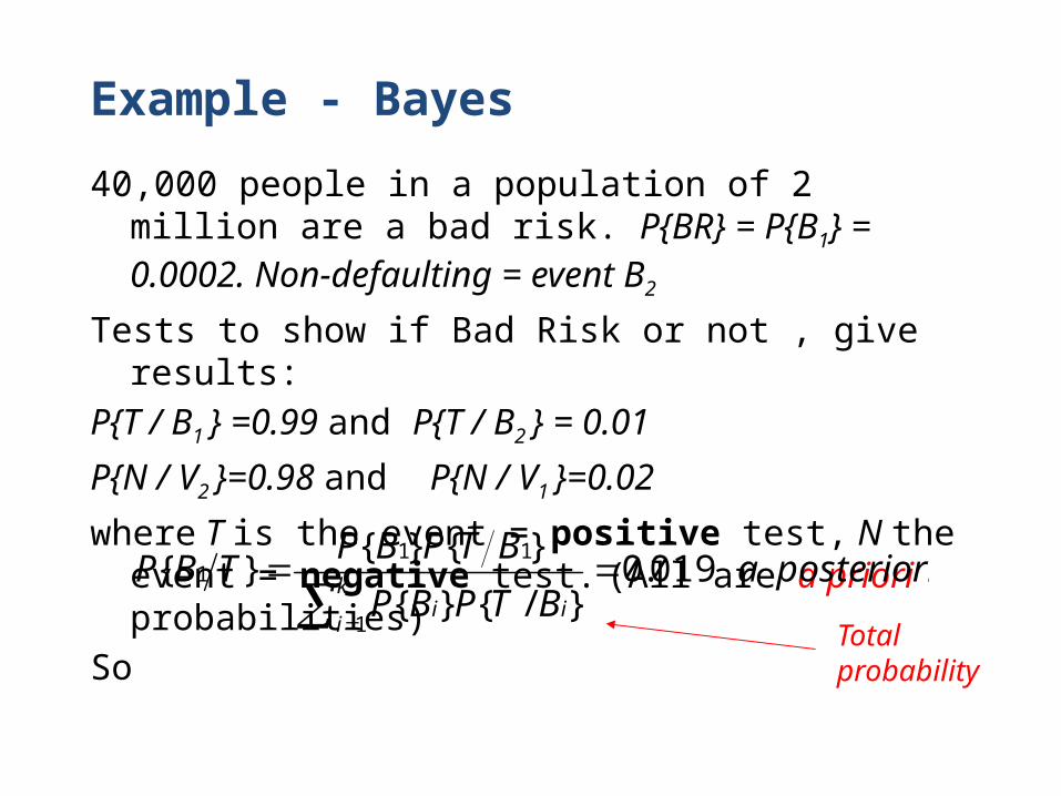
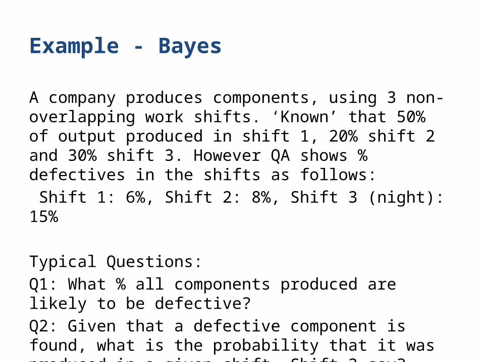
Example - Bayes
40,000 people in a population of 2 million are a bad risk. P{BR} = P{B1} = 0.0002. Non-defaulting = event B2
Tests to show if Bad Risk or not , give results:P{T / B1 } =0.99 and P{T / B2 } = 0.01
P{N / V2 }=0.98 and P{N / V1 }=0.02
where T is the event = positive test, N the event = negative test. (All are a priori probabilities)
So
where events Bi partition the sample space
posterioriaBTPBP
BTPBPTBP k
iii
019.0}/{}{
}{}{}{
1
111
Total probability
Example - Bayes
A company produces components, using 3 non-overlapping work shifts. ‘Known’ that 50% of output produced in shift 1, 20% shift 2 and 30% shift 3. However QA shows % defectives in the shifts as follows: Shift 1: 6%, Shift 2: 8%, Shift 3 (night): 15%
Typical Questions:Q1: What % all components produced are likely to be defective?Q2: Given that a defective component is found, what is the probability that it was produced in a given shift, Shift 3 say?
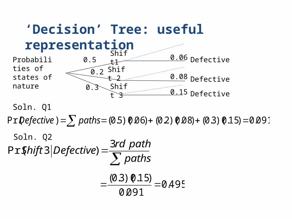
‘Decision’ Tree: useful representation
0.2
0.5
0.3
Shift1
Shift 2
Shift 3
0.06
0.08
0.15
Defective
Defective
Defective
091.0)15.0)(3.0()08.0)(2.0()06.0)(5.0()Pr( pathsDefective
paths
pathrdDefectiveShift
3)3Pr(
495.0091.0
)15.0)(3.0(
Probabilities of states of nature
Soln. Q1
Soln. Q2
8
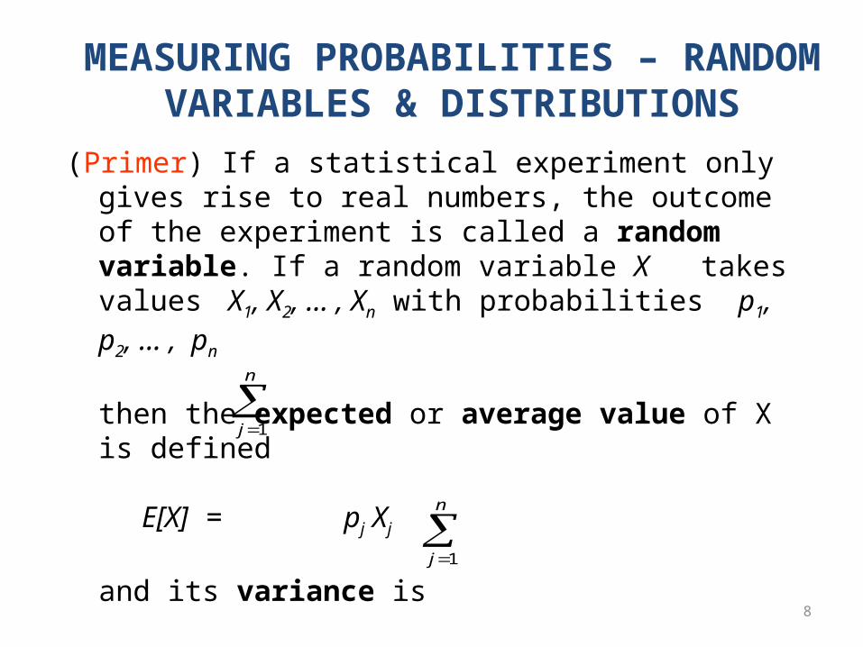
MEASURING PROBABILITIES – RANDOM VARIABLES & DISTRIBUTIONS
(Primer) If a statistical experiment only gives rise to real numbers, the outcome of the experiment is called a random variable. If a random variable X takes values X1, X2, … , Xn with probabilities p1, p2, … , pn
then the expected or average value of X is defined
E[X] = pj Xj
and its variance is
VAR[X] = E[X2] - E[X]2 = pj Xj2 - E[X]2
j
n
1
j
n
1
9
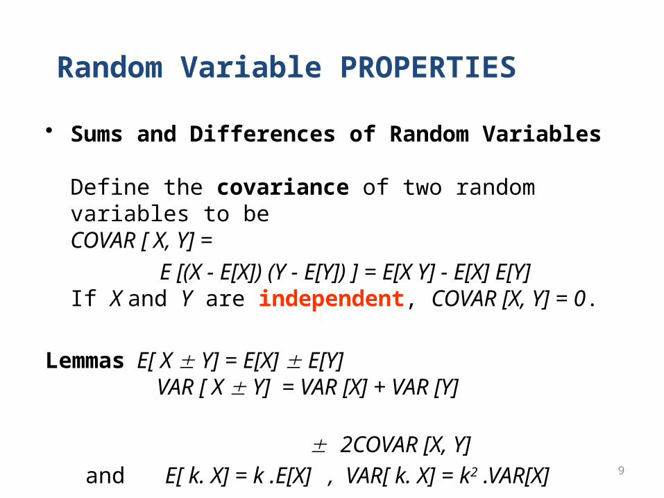
Random Variable PROPERTIES
• Sums and Differences of Random Variables
Define the covariance of two random variables to be COVAR [ X, Y] =
E [(X - E[X]) (Y - E[Y]) ] = E[X Y] - E[X] E[Y]If X and Y are independent, COVAR [X, Y] = 0.
Lemmas E[ X Y] = E[X] E[Y] VAR [ X Y] = VAR [X] + VAR [Y]
2COVAR [X, Y] and E[ k. X] = k .E[X] , VAR[ k. X] = k2 .VAR[X] for a constant k.
10
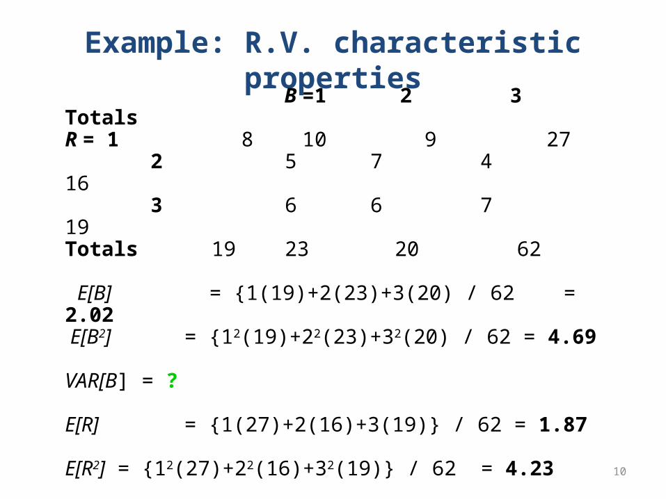
Example: R.V. characteristic properties
B =1 2 3 TotalsR = 1 8 10 9 27 2 5 7 4 16 3 6 6 7 19Totals 19 23 20 62
E[B] = {1(19)+2(23)+3(20) / 62 = 2.02 E[B2] = {12(19)+22(23)+32(20) / 62 = 4.69
VAR[B] = ?
E[R] = {1(27)+2(16)+3(19)} / 62 = 1.87 E[R2] = {12(27)+22(16)+32(19)} / 62 = 4.23
VAR[R] = ?
11
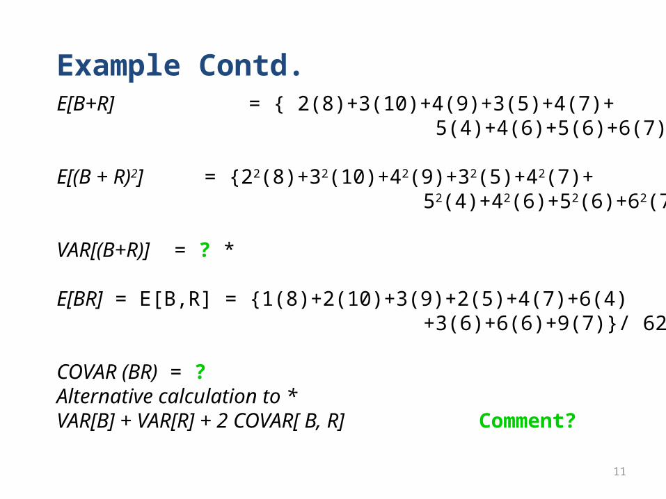
Example Contd.E[B+R] = { 2(8)+3(10)+4(9)+3(5)+4(7)+ 5(4)+4(6)+5(6)+6(7)} / 62 = 3.89
E[(B + R)2] = {22(8)+32(10)+42(9)+32(5)+42(7)+ 52(4)+42(6)+52(6)+62(7)} / 62 = 16.47
VAR[(B+R)] = ? *
E[BR] = E[B,R] = {1(8)+2(10)+3(9)+2(5)+4(7)+6(4) +3(6)+6(6)+9(7)}/ 62 = 3.77 COVAR (BR) = ?Alternative calculation to * VAR[B] + VAR[R] + 2 COVAR[ B, R] Comment?
12
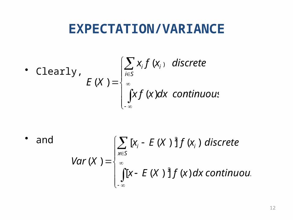
EXPECTATION/VARIANCE
• Clearly,
• and
continuousdxxfx
discretexfx
XESi
ii
)(
(
)(
)
continuousdxxfXEx
discretexfXEx
XVarSx
ii
)()]([
)()]([
)(2
2
13
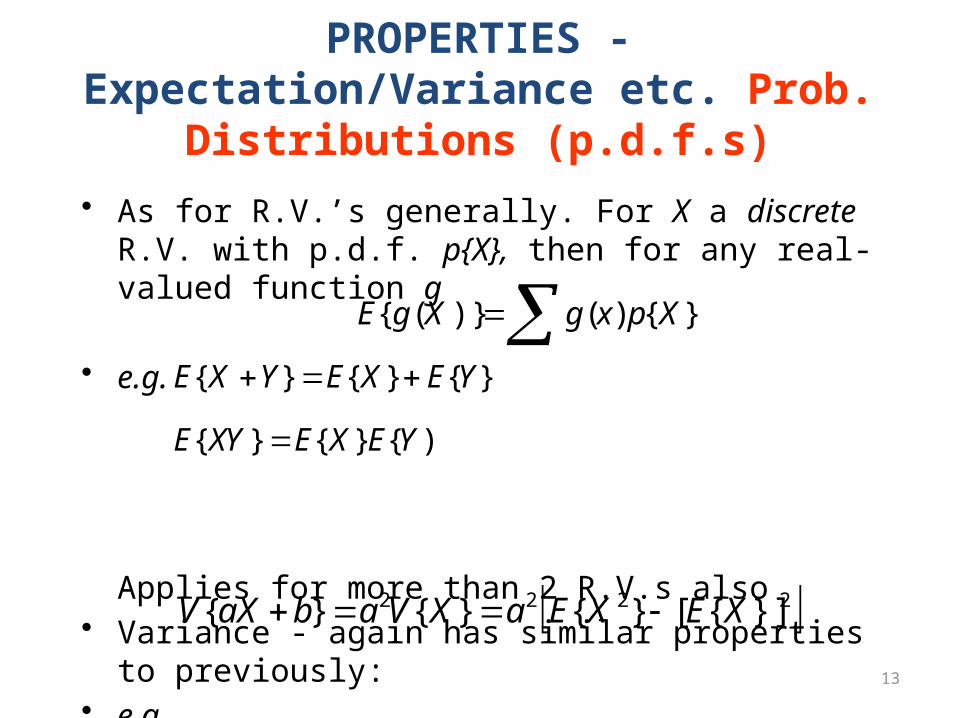
PROPERTIES - Expectation/Variance etc. Prob. Distributions (p.d.f.s)
• As for R.V.’s generally. For X a discrete R.V. with p.d.f. p{X}, then for any real-valued function g
• e.g.
Applies for more than 2 R.V.s also• Variance - again has similar properties to previously:• e.g.
}{)()}({ XpxgXgE
){}{}{
}{}{}{
YEXEXYE
YEXEYXE
2222 }]{[}{}{}{ XEXEaXVabaXV
14
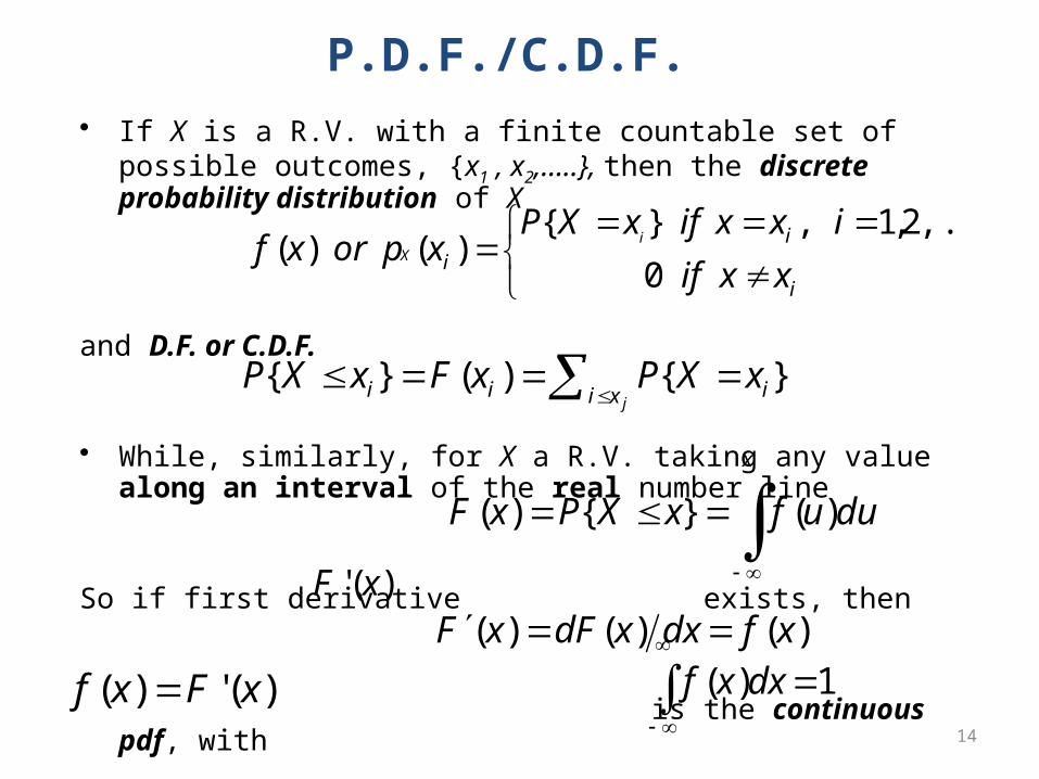
P.D.F./C.D.F.• If X is a R.V. with a finite countable set of possible outcomes, {x1 , x2,
…..}, then the discrete probability distribution of X
and D.F. or C.D.F.
• While, similarly, for X a R.V. taking any value along an interval of the real number line
So if first derivative exists, then
is the continuous pdf, with
i
ii xxif
ixxifxXPxporxf i
X
0
,....2,1,}{)()(
jxi iii xXPxFxXP }{)(}{
x
duufxXPxF )(}{)(
)()()( xfdxxdFxF
1)( dxxf
)(' xF
)(')( xFxf
15
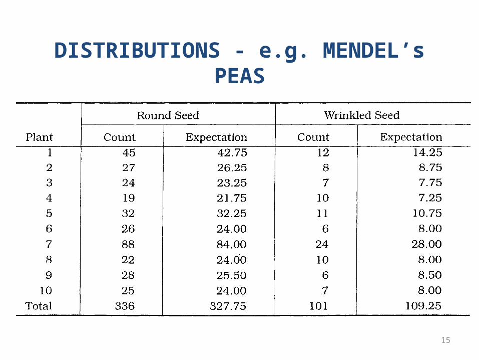
DISTRIBUTIONS - e.g. MENDEL’s PEAS
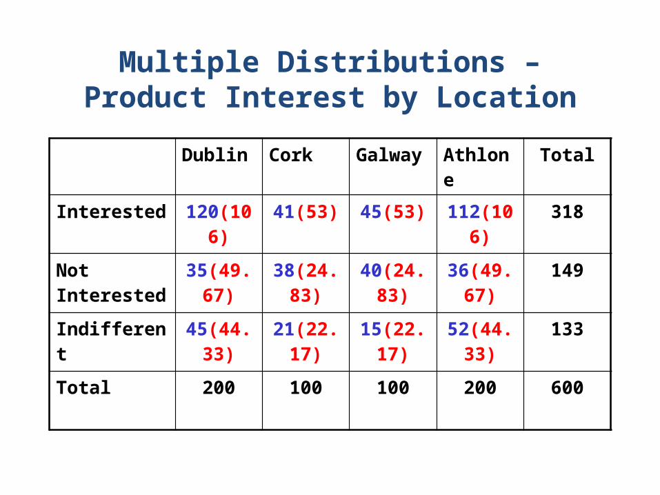
Multiple Distributions – Product Interest by Location
Dublin Cork Galway Athlone Total
Interested 120(106) 41(53) 45(53) 112(106) 318
Not Interested
35(49.67) 38(24.83) 40(24.83) 36(49.67) 149
Indifferent 45(44.33) 21(22.17) 15(22.17) 52(44.33) 133
Total 200 100 100 200 600
17
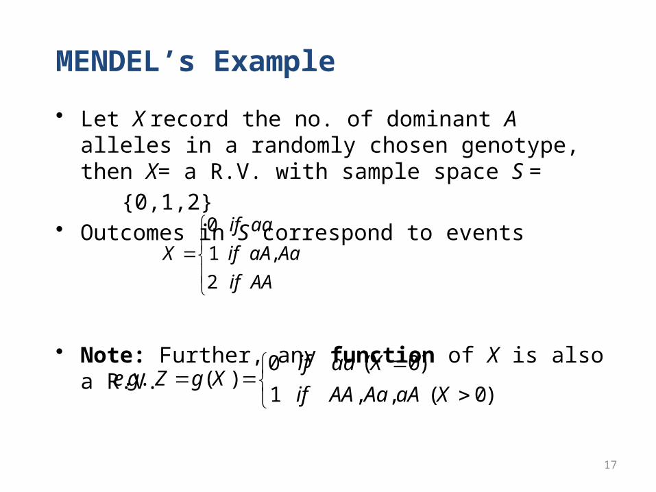
MENDEL’s Example
• Let X record the no. of dominant A alleles in a randomly chosen genotype, then X= a R.V. with sample space S =
{0,1,2}• Outcomes in S correspond to events
• Note: Further, any function of X is also a R.V.
• Where Z is a variable for seed character phenotype
AAif
AaaAif
aaif
X
2
,1
0
)0(,,1
)0(0)(..
XaAAaAAif
XaaifXgZge
18
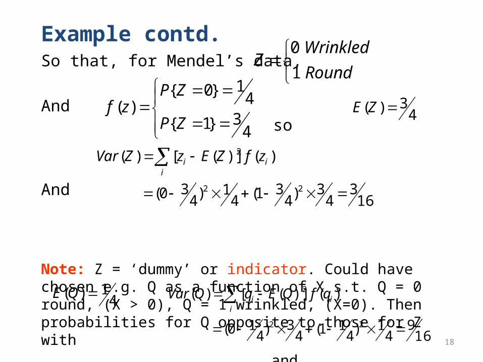
Example contd.So that, for Mendel’s data,
And so And
Note: Z = ‘dummy’ or indicator. Could have chosen e.g. Q as a function of X s.t. Q = 0 round, (X > 0), Q = 1 wrinkled, (X=0). Then probabilities for Q opposite to those for Z with and
Round
WrinkledZ
1
0
43}1{
41}0{
)(ZP
ZPzf 4
3)( ZE
163
43)4
31(41)4
30(
)()]([)(
22
2
i
ii zfZEzZVar
41)( QE
169
41)4
11(43)4
10(
)()]([)(
22
2
i
ii qfQEqQVar
19
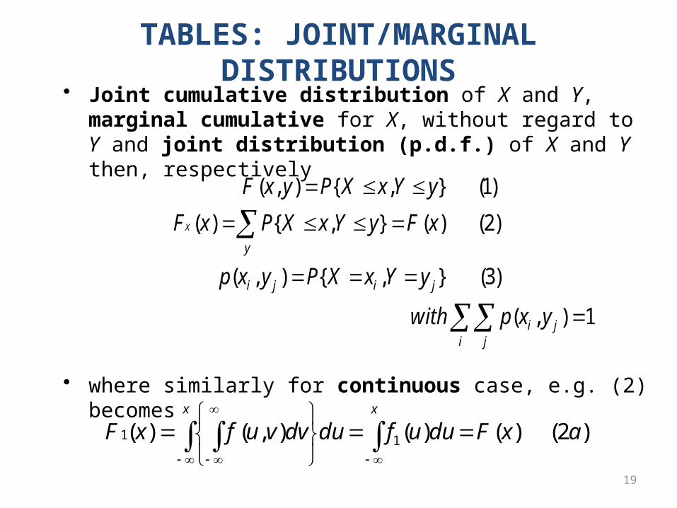
TABLES: JOINT/MARGINAL DISTRIBUTIONS• Joint cumulative distribution of X and Y, marginal cumulative for
X, without regard to Y and joint distribution (p.d.f.) of X and Y then, respectively
• where similarly for continuous case, e.g. (2) becomes
1),(
)3(},{),(
)2()(},{)(
)1(},{),(
i jji
jiji
y
yxpwith
yYxXPyxp
xFyYxXPxF
yYxXPyxF
X
)2()()(),()( 11 axFduufdudvvufxFxx
20
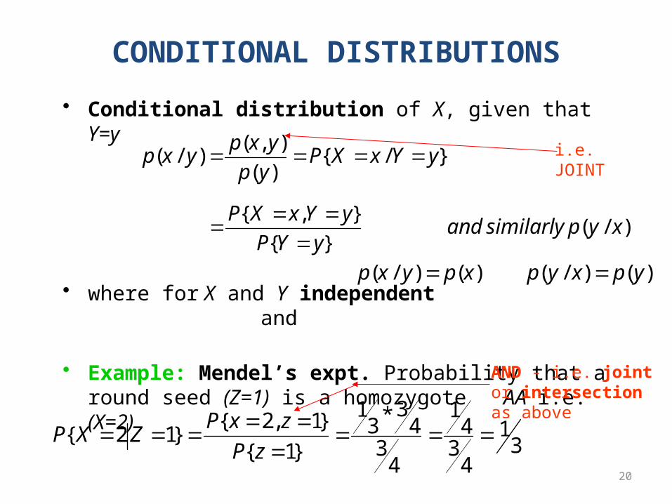
CONDITIONAL DISTRIBUTIONS
• Conditional distribution of X, given that Y=y
• where for X and Y independent and
• Example: Mendel’s expt. Probability that a round seed (Z=1) is a homozygote AA i.e. (X=2)
)/(}{
},{
}/{)(
),()/(
xypsimilarlyandyYP
yYxXP
yYxXPyp
yxpyxp
)()/( xpyxp )()/( ypxyp
31
43
41
43
43*3
1
}1{
}1,2{}12{
zP
zxPZXP
AND - i.e. joint or intersection as above
i.e. JOINT
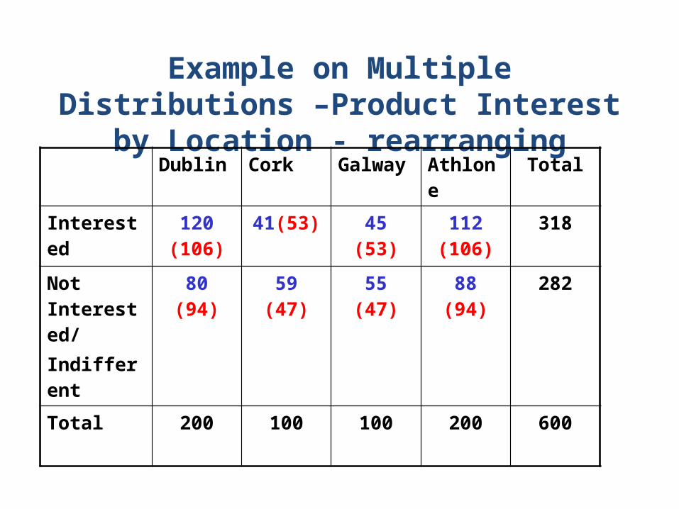
Example on Multiple Distributions –Product Interest by Location - rearranging
Dublin Cork Galway Athlone Total
Interested 120 (106) 41(53) 45 (53) 112 (106) 318
Not Interested/Indifferent
80 (94) 59 (47) 55 (47) 88 (94) 282
Total 200 100 100 200 600
BAYES Developed Example: Business Informatics
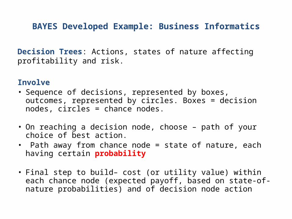
Decision Trees: Actions, states of nature affecting profitability and risk.
Involve• Sequence of decisions, represented by boxes, outcomes, represented
by circles. Boxes = decision nodes, circles = chance nodes.
• On reaching a decision node, choose – path of your choice of best action.
• Path away from chance node = state of nature, each having certain probability
• Final step to build– cost (or utility value) within each chance node (expected payoff, based on state-of-nature probabilities) and of decision node action

Example• A Company wants to market a new line of computer tablets. Main
concern is price to be set and for how long. Managers have a good idea of demand at each price, but want to get an idea of time it will take competitors to catch up with a similar product. Would like to retain a price for 2 years.
• Decision problem: 4 possible alternatives say: A1: price €1500, A2 price €1750, A3: price €2000 A4: price €2500.
• State-of-nature = catch up times: S1 : < 6 months, S2: 6-12 months, S3: 12-18 months, S4: > 18 months.
• Past experience indicates P{S1}= 0.1, P{S2}=0.5,P{S3}=0.3, P{S4)=0.1
• Need costs (payoff table) for various strategies ; non-trivial since involves price-demand, cost-volume, consumer preference info. etc. involved to specify payoff for each action. Conservative strategy = minimax, Risky strategy = maximise expected payoff
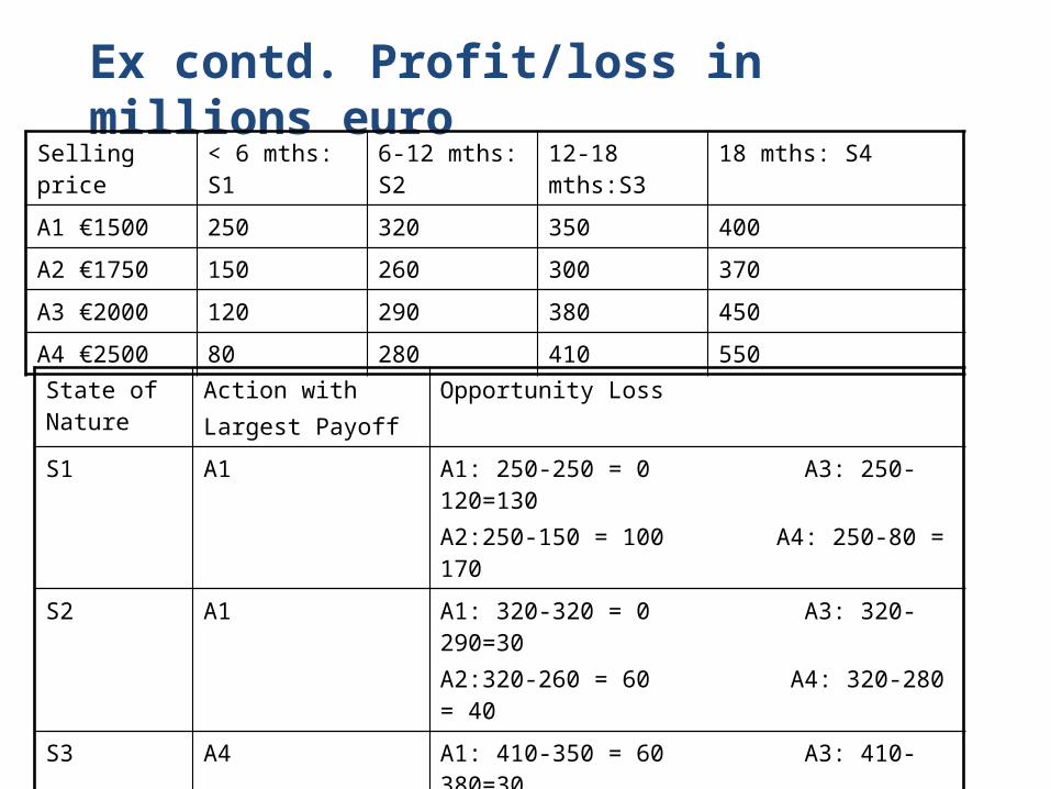
Ex contd. Profit/loss in millions euro
Selling price < 6 mths: S1 6-12 mths: S2 12-18 mths:S3 18 mths: S4
A1 €1500 250 320 350 400
A2 €1750 150 260 300 370
A3 €2000 120 290 380 450
A4 €2500 80 280 410 550
State of Nature
Action with Largest Payoff
Opportunity Loss
S1 A1 A1: 250-250 = 0 A3: 250-120=130A2:250-150 = 100 A4: 250-80 = 170
S2 A1 A1: 320-320 = 0 A3: 320-290=30A2:320-260 = 60 A4: 320-280 = 40
S3 A4 A1: 410-350 = 60 A3: 410-380=30A2: 410-300 = 110 A4: 410-410 = 0
S4 A4 A1: 550-400 = 60 A3: 550-450=30A2: 550-370 = 110 A4: 550-550 = 0
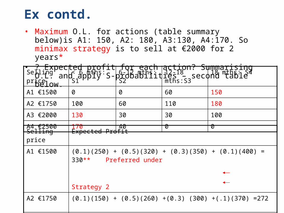
Ex contd.• Maximum O.L. for actions (table summary below)is A1: 150, A2: 180,
A3:130, A4:170. So minimax strategy is to sell at €2000 for 2 years*• ? Expected profit for each action? Summarising O.L. and apply S-
probabilities – second table below.
* Suppose want to maximise minimum payoff, what changes? (maximin strategy)
Selling price < 6 mths: S1 6-12 mths: S2 12-18 mths:S3 18 mths: S4
A1 €1500 0 0 60 150
A2 €1750 100 60 110 180
A3 €2000 130 30 30 100
A4 €2500 170 40 0 0
Selling price Expected Profit
A1 €1500 (0.1)(250) + (0.5)(320) + (0.3)(350) + (0.1)(400) = 330** Preferred under Strategy 2
A2 €1750 (0.1)(150) + (0.5)(260) +(0.3) (300) +(.1)(370) =272
A3 €2000 (0.1)(120) + (0.5)(290) + (0.3)(380) + (0.1)450) = 316 but
A4 €2500 (0.1)(80) + (0.5)(280) +(0.3)(410) +(0.1)(550) = 326 but
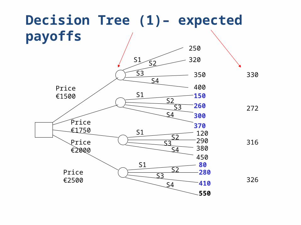
Decision Tree (1)– expected payoffs
250
320
350
400
370
150260300
12029038045080280
410550
Price €1500
Price €1750
Price €2000
Price €2500
S1 S2S3
S4
S1
S1
S1
S2
S2
S2
S3
S3
S3
S4
S4
S4
330
272
316
326
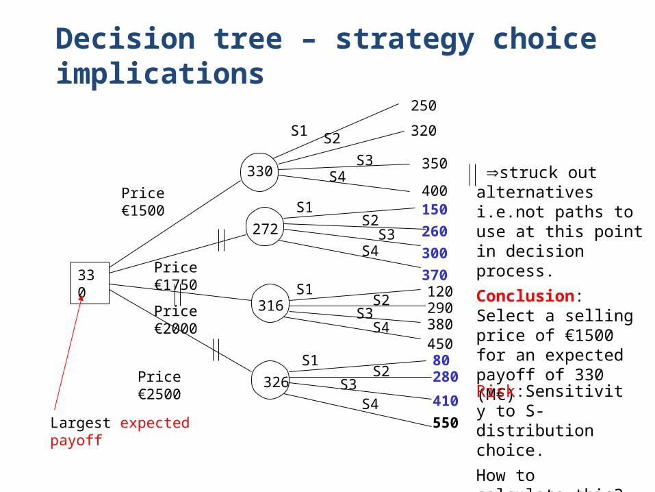
Decision tree – strategy choice implications
250
320
350
400
370
150260300
12029038045080280
410550
Price €1500
Price €1750
Price €2000
Price €2500
S1 S2S3
S4
S1
S1
S1
S2
S2
S2
S3
S3
S3
S4
S4
S4
330
330
272
316
326
Largest expected payoff
struck out alternatives i.e.not paths to use at this point in decision process.
Conclusion: Select a selling price of €1500 for an expected payoff of 330 (M€)
Risk:Sensitivity to S-distribution choice.
How to calculate this?
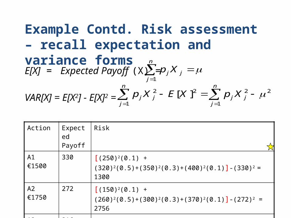
Example Contd. Risk assessment – recall expectation and variance forms
E[X] = Expected Payoff (X) =
VAR[X] = E[X2] - E[X]2 =
j
n
jj Xp
1
22
1
22
1
][
j
n
jjj
n
jj XpXEXp
Action Expected Payoff
Risk
A1 €1500 330 [(250)2(0.1) + (320)2(0.5)+(350)2(0.3)+(400)2(0.1)]-(330)2 = 1300
A2 €1750 272 [(150)2(0.1) + (260)2(0.5)+(300)2(0.3)+(370)2(0.1)]-(272)2 = 2756
A3 €2000 316 [(120)2(0.1) + (290)2(0.5)+(380)2(0.3)+(450)2(0.1)]-(316)2 = 7204
A4 €2500 326 [(80)2(0.1) + (280)2(0.5)+(410)2(0.3)+(550)2(0.1)]-(326)2 =14244
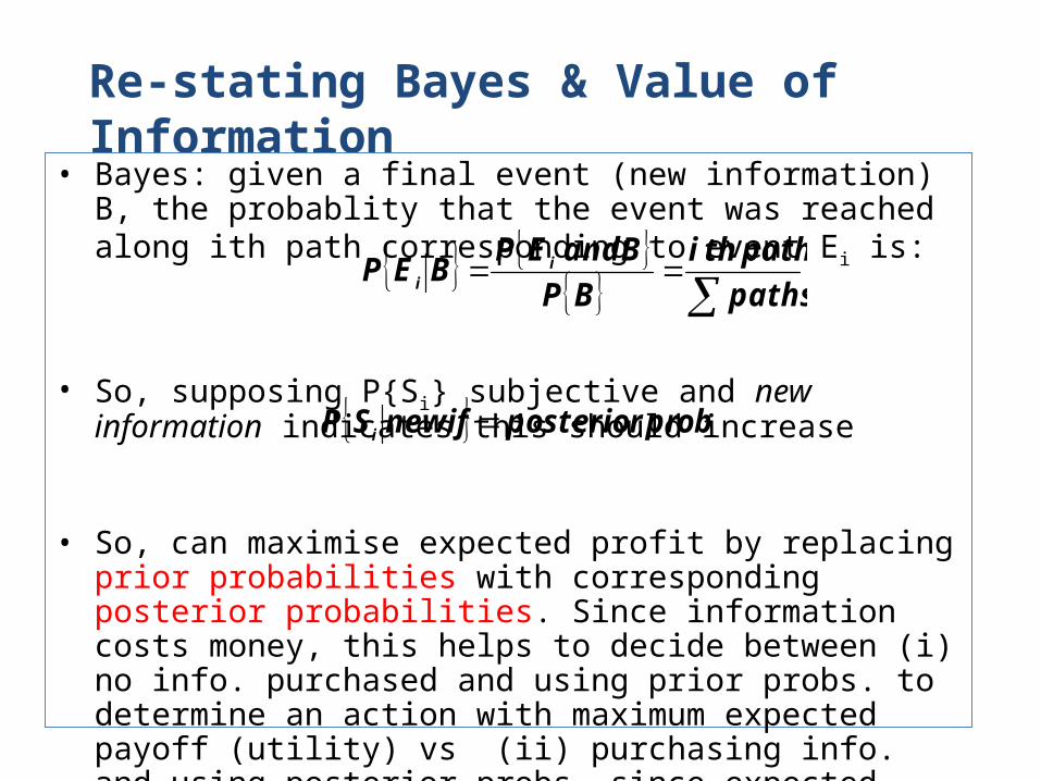
Re-stating Bayes & Value of Information
• Bayes: given a final event (new information) B, the probablity that the event was reached along ith path corresponding to event Ei is:
• So, supposing P{Si} subjective and new information indicates this should increase
• So, can maximise expected profit by replacing prior probabilities with corresponding posterior probabilities. Since information costs money, this helps to decide between (i) no info. purchased and using prior probs. to determine an action with maximum expected payoff (utility) vs (ii) purchasing info. and using posterior probs. since expected payoff (utility) for this decision could be larger than that obtained using prior probs only.
paths
paththi
BP
BandEPBEP i
i
probposteriornewifSP i
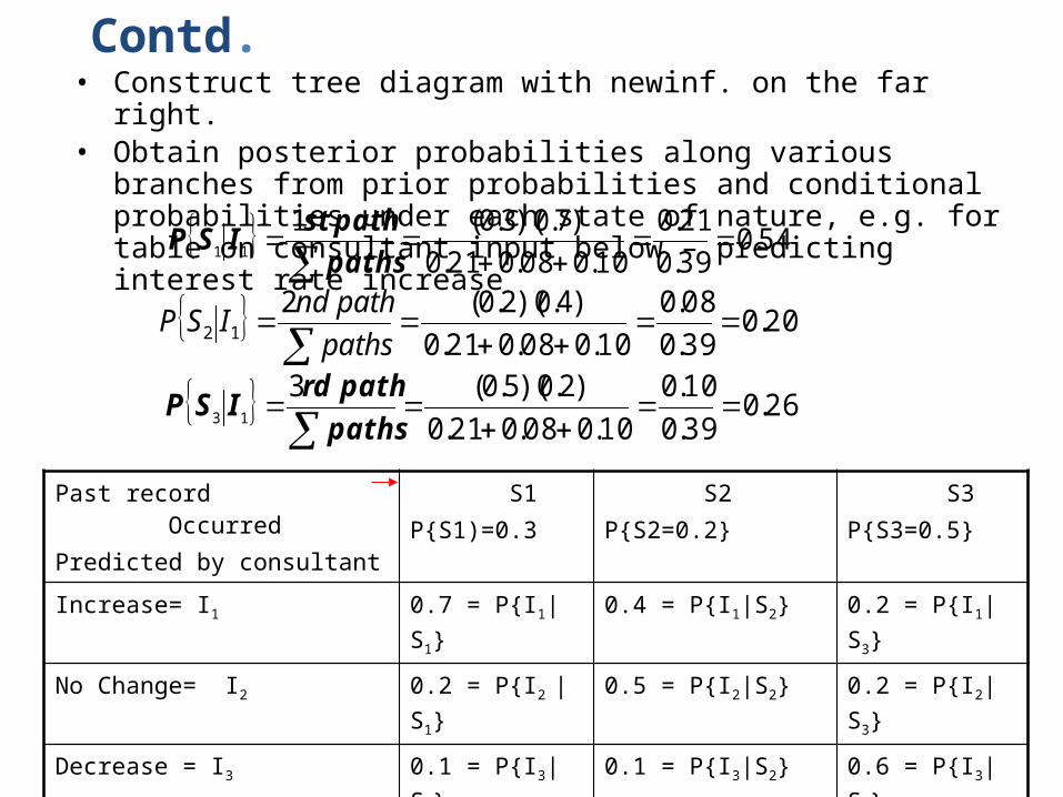
Contd.• Construct tree diagram with newinf. on the far right. • Obtain posterior probabilities along various branches from prior
probabilities and conditional probabilities under each state of nature, e.g. for table on consultant input below – predicting interest rate increase
• Expected payoffs etc. now calculated using the posterior probabilities
Past record OccurredPredicted by consultant
S1P{S1)=0.3
S2P{S2=0.2}
S3P{S3=0.5}
Increase= I1 0.7 = P{I1|S1} 0.4 = P{I1|S2} 0.2 = P{I1|S3}
No Change= I2 0.2 = P{I2 |S1} 0.5 = P{I2|S2} 0.2 = P{I2|S3}
Decrease = I3 0.1 = P{I3|S1} 0.1 = P{I3|S2} 0.6 = P{I3|S3}
1.0 1.0 1.0
54.039.0
21.0
10.008.021.0
)7.0)(3.0(111
paths
pathstISP
20.039.0
08.0
10.008.021.0
)4.0)(2.0(212
paths
pathndISP
26.039.0
10.0
10.008.021.0
)2.0)(5.0(313
paths
pathrdISP
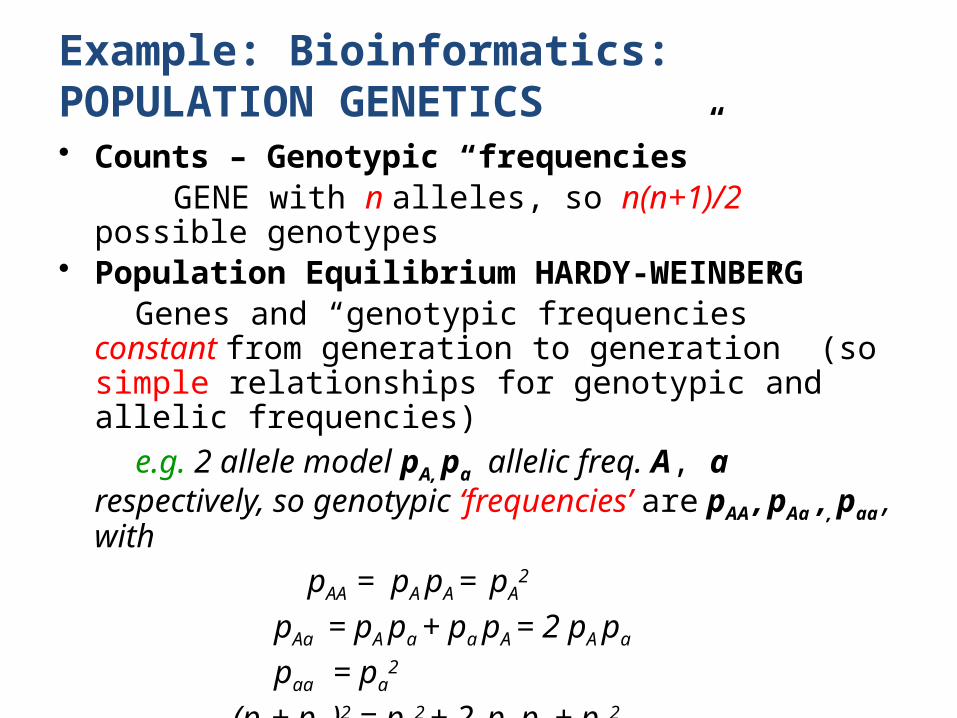
Example: Bioinformatics: POPULATION GENETICS
• Counts – Genotypic “frequencies” GENE with n alleles, so n(n+1)/2 possible genotypes • Population Equilibrium HARDY-WEINBERG Genes and “genotypic frequencies” constant from generation
to generation (so simple relationships for genotypic and allelic frequencies)
e.g. 2 allele model pA, pa allelic freq. A, a respectively, so genotypic ‘frequencies’ are pAA , pAa ,, paa , with
pAA = pA pA = pA2
pAa = pA pa + pa pA = 2 pA pa
paa = pa2
(pA+ pa )2 = pA2 + 2 pa pA + pa
2
One generation of Random mating. H-W at single locus
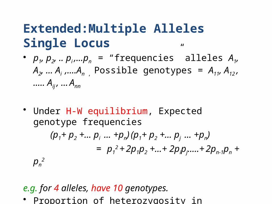
Extended:Multiple Alleles Single Locus
• p1, p2, .. pi ,...pn = “frequencies” alleles A1, A2, … Ai ,….An ,
Possible genotypes = A11, A12 , ….. Aij , … Ann
• Under H-W equilibrium, Expected genotype frequencies (p1+ p2 +… pi ... +pn) (p1+ p2 +… pj ... +pn)
= p12
+ 2p1p2 +…+ 2pipj…..+ 2pn-1pn + pn2
e.g. for 4 alleles, have 10 genotypes.• Proportion of heterozygosity in population clearly PH = 1 -i p i
2 used in screening of
genetic markers
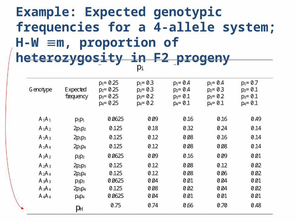
Example: Expected genotypic frequencies for a 4-allele system; H-W m, proportion of heterozygosity in F2 progeny
pi
Genotype Expectedfrequency
p1= 0.25p2= 0.25p3= 0.25p4= 0.25
p1= 0.3p2= 0.3p3= 0.2p4= 0.2
p1= 0.4p2= 0.4p3= 0.1p4= 0.1
p1= 0.4p2= 0.3p3= 0.2p4= 0.1
p1= 0.7p2= 0.1p3= 0.1p4= 0.1
A1A1 p1p1 0.0625 0.09 0.16 0.16 0.49
A1A2 2p1p2 0.125 0.18 0.32 0.24 0.14
A1A3 2p1p3 0.125 0.12 0.08 0.16 0.14
A1A4 2p1p4 0.125 0.12 0.08 0.08 0.14
A2A2 p2p2 0.0625 0.09 0.16 0.09 0.01
A2A3 2p2p3 0.125 0.12 0.08 0.12 0.02A2A4 2p2p4 0.125 0.12 0.08 0.06 0.02A3A3 p3p3 0.0625 0.04 0.01 0.04 0.01A3A4 2p3p4 0.125 0.08 0.02 0.04 0.02A4A4 p4p4 0.0625 0.04 0.01 0.01 0.01
pH0.75 0.74 0.66 0.70 0.48
34
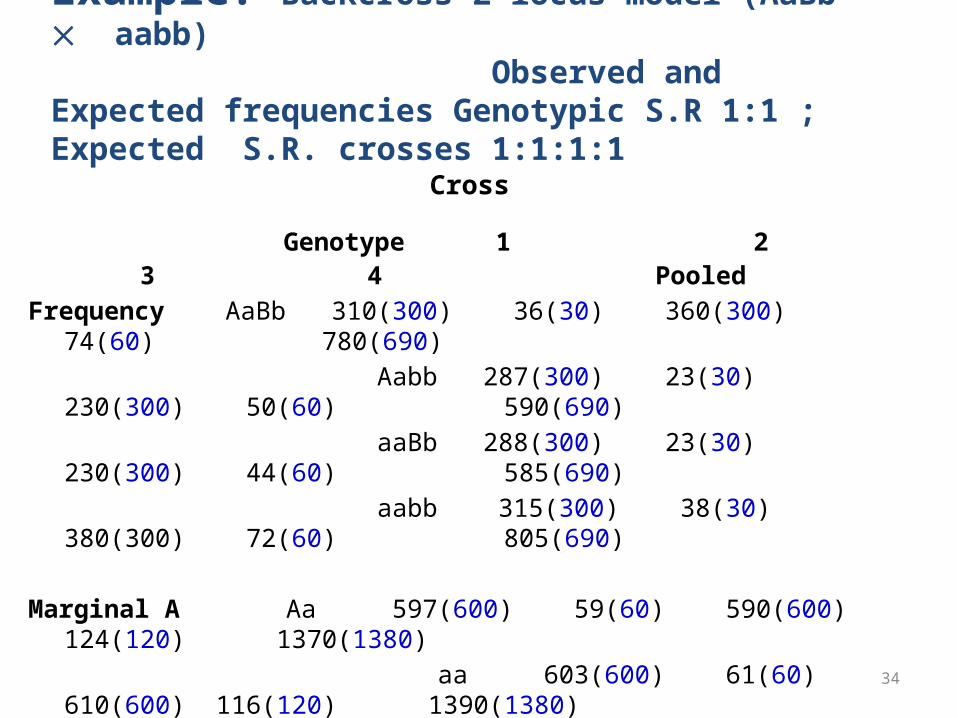
Example: Backcross 2 locus model (AaBb aabb) Observed and Expected frequencies Genotypic S.R 1:1 ; Expected S.R. crosses 1:1:1:1
Cross
Genotype 1 2 3 4 Pooled
Frequency AaBb 310(300) 36(30) 360(300) 74(60) 780(690) Aabb 287(300) 23(30) 230(300) 50(60) 590(690) aaBb 288(300) 23(30) 230(300) 44(60) 585(690) aabb 315(300) 38(30) 380(300) 72(60) 805(690)
Marginal A Aa 597(600) 59(60) 590(600) 124(120) 1370(1380) aa 603(600) 61(60) 610(600) 116(120) 1390(1380)
Marginal B Bb 598(600) 59(60) 590(600) 118(120) 1365(1380) bb 602(600) 61(60) 610(600) 122(120) 1395(1380) Sum 1200 120 1200 240 2760