Embed Size (px)
Citation preview
International Journal of Engineering Research and Technology.
ISSN 0974-3154 Volume 11, Number 2 (2018), pp. 333-348
© International Research Publication House
http://www.irphouse.com
Data Analysis Utilizing Principal Component
Analysis
Bhawana Mathur1, Manju Kaushik2
1,2Department of Computer Science & Engineering, JECRC University, Jaipur (India)
Corresponding address: 9660676022, [email protected]
Abstract
More information is collected from a population. The purpose of the research
is that the covariance matrix or correlation matrix has been detected by
principal component analysis. These major component scores have been used
in further investigation. This work has been done by the Principal Component
Analysis (PCA) and the calculation of Change- proneness of both the software
has been calculated. PCA technology enhances the quality of the software in
this paper. This is a data-dimensional reduction method. The main purpose of
PCA is to understand many versions of software and complete software
process. This software is used in client applications. PCA algorithm which
reduces large amounts of information in 2-dimensional. Here we have used
object-oriented software which is built in the Ada language. These are two
commercial software UIMS (User Interface System) and QUES (Quality
Assessment System) whose best source code metrics and maintenance are
calculated. QUES has 71 examples and 11 features. There are 39 instances and
features in UIMS. Software quality has been earned by seven classified
techniques like IBK, Multilayer Perceptron, Simple Linear Regression,
Decision Table, Decision Stump, RBF Network and Gaussian Process.
Keywords: Principal component analysis, Software, Change-proneness,
Software quality, Mean Absolute Error, Root Mean Square Error.
I. INTRODUCTION
In this work, we have assessed the data set through Principal Component Analysis
(PCA). It is extremely difficult to understand the information in sufficient quantities
as well as it is exceptionally difficult too. At present, Principal Component Analysis
(PCA) is a basic mechanism in different areas of computer graphics from
neuroscience. This is a basic, non-parametric strategy for mining (Erkmann and
334 Bhawana Mathur, Manju Kaushik
Yelirim, 2008). PCA provides standard for reducing a complex data set. The purpose
of research is to cooperate with PCA. We are working through numerical values so
that it can provide a clear solution to the directly convertible system on the basis of
mathematics. PCA and machine learning detected dimensional deficiencies by USE.
The variation in the variation in the software is an important marker to affect the
software feature. Subtracting, adding and updating have increased the quality of
software, which depends on the development of software. There is some change-
specificity in this excellent software. When customers have time to get the
requirement, all the expenses incurred are within the scheme. At the same time they
have resolved the issues of the customers. Programming engineers have the ability to
detect various types of change-prone possibilities. Explained the clear-cut clarity
pattern that used the areas where there is change-nature. Understand the fundamental
explanation behind the change. Recommended to include change specificity and
reduce the amount of change-nature. Scholars have examined the components that are
the result of change, and changes in software - exploration investigation has examined
specificity for some important elements. Despite the measures indicated by these key
elements, they progressed in the testing process. As well as increasing the
programming quality, the nature of nature is adequately kept. During the software
development process, the software has improved "spin-off" and software-changes.
There is a sequence of achievements in the Change-Shield Test (Guo, 2016). It has
also made significant accumulation of software improvements with change-specificity
and it has been created in a new way. Data-specificity calculation, outline data, logical
information of checker indicator is collected. Regarding regression testing on drip
change-prone regression, with the designer unit testing, the regression has been
studied. Analyze the root cause for changing the focus of change causes. To focus on
the change, the variations separated by circulation-the type of shield and the original
change-unity are separated (K-Gang, LHH, 200 9). Testing of patterns has been
disconnected about two important patterns in the testing process: a trend is change-the
amount of singularity, as well as the amount of renewal in other patterns. Various
investigations on the investigation of Change -prone causes have been done. The
examination of Change-proneness reasons of root cause, all in all Change-proneness
classification (Jayatilleke and Lai, 2017) as well as examination of software Change-
proneness influence -factors depend of Bayesian Formula (Gatrell, 2012). The
technology of Bayesian Formula has been used to check all software variation-type
factors. Variations vary on classic PCA method for different classes. PCA technology
reduces information without losing specificity. The process continues, reducing the
size of the dataset and without losing the main sections. Despite this fact, the PCA is
also a development system, which is still difficult to give the reality to the algorithm.
Especially during adjusting it to different types of information, or during
preprocessing, the result is included in the generation stages. UIMS (User Interface
System) and QUES (Quality Assessment System) are published by Li and Henry
(1993). The software shows many varieties of fundamental progress and PCA also
provide better results. The fundamental commitments shown in this paper are:
1. A top composition strategy;
2. Using the structure; Plus
Data Analysis Utilizing Principal Component Analysis 335
3. Wilmott and Matsuara (2005) have suggested that RMSE is not a good
indicator of general model performance and average error can also be
misleading, hence the MAE is a better metric (Wilmott and Matsuara, 2005).
Change-proneness is an important external quality attribute that denotes the extent of
change of a class across the versions of the system. Change-proneness values are
calculated using number of SLOC changes. According to Li and Henry (1) each added
or deleted source code line has been counted as one SLOC change; (2) each modified
source code line has been counted as two SLOC change.
II. RELATED WORK
Information about the software is indicated by change-specificity. Software engineers
could not understand the issues of customers (Ernst, 2012). According to ISO 9000,
change-specificity is a feature of software. For example, changes-requirements are
important for important requirements and predefined uses (Kovacs and Sasabad,
2013). Change-specificity is a piece of programming that exists in the product. It has
been replaced by some source code metrics in the product. To predict the change-
prone of the product (Koru and Liu, 2007), different creators have suggested.
Techniques for creating a change-prone forecast model are different from the process
of regression testing by learning machine, For example, neural networks. In addition
to source-code metrics, apply some compulsory checks to create prediction, prediction
models. Henry and Kefura examined the correlation of the source code metric (Kafura
and Henry, 1981) and changed the number of source code to measure the correlation
between the changes of the Unix operating structure. They found that source code is
correlated strongly with Metrics Diversity (Kumar et al., 2017). Ruchika and
Anuradha examined the relationship between object-oriented metrics as well as the
maintenance of the source code metrics of different types of software (Malhotra and
Chugh, 2016) (Chidambar and Kemer, 1994). They calculate source code metrics by
new and old applications to check the amendments made in each class. The software
expert used the object-oriented source code metric to predict the maintenance of the
software framework (Kumar et al., 2017). Ah-Rim Han et al suggested metrics to
measure the structural and behavioral dependencies of UML 2.0 (Han, et al., 2010).
For high-quality software, the design-model of change-specificity has been used in the
first stage of the software development process and it is believed that source code
metrics are a useful indicator. After the structure, the structure and prediction of high
level polymorphism with frame-virtual relationships can be different from the current
object-oriented metric. Sixty object-oriented code metrics were taken to predict
changes (Lu et al, 2012). Find results by meta-analysis strategies.
In its work, the characteristic of change-prone is that a class which can change the
structure in the following form. Consolidates four separate metric dimensions for the
search of object-oriented source code metrics (Kumar and Suraka, 2017) Like
cohesion, coupling, size, as well as inheritance. Ying and Harrton created a predictive
model for the maintenance of software using software metrics. For which many
336 Bhawana Mathur, Manju Kaushik
adaptive regression splinces (MARS) discussed the modeling methods (Chen and
Huang, 2009), (Zhou and Leung, 2007).
This software metrics information has been collected from two different object-
oriented frameworks. They also focus on the use of assessing the performance of
MARS models as well as regression tree model, artificial neural network model,
multivariate linear regression models, as well as support vector model (Kumar and
Sureka, 2017). They found that models using MARS have compared more than the
other four specific modeling strategies to more precise predictions, and then MARS
for other systems is accurate as the best modeling strategies. The authors discussed
the specific set of source code metrics to predict the change-proneness of object-
oriented software. This indicates that the change -prone forecast model depends on
the display source code metric. The source code metric has been used as the input to
model. Determining the appropriate set is an essential stage of data checking in
different areas. Feature selection techniques have been used in literature in different
areas (Wang, et. al., 1997).
In this work, the selection methods of the five specific types of characteristics, for
example, univariate logistic regression analysis, gain ratio feature evaluation,
information gain feature evaluation, principal component analysis (PCA), as well as
rough set analysis (RSA) has been used by which to find the correct subsets of
software metrics. In this work, we consider four different metric dimensions, for
example, size, cohesion, coupling as well as inheritance source code metrics, to assess
the effectiveness of these different dimension metrics on the change- proneness of
object-oriented software (Sharafat, and Tahvildari, 2008). In these tests, eight
different machine learning algorithms have been used to evaluate the effectiveness of
these sets of source code metrics such as LOGR, NBC, ELM-LIN, ELM-PLY, ELM-
RBF, SVM-LIN, SVM-RBF, SVMSIG and two ensemble methods, for example,
Best-in-Training (BTE) and majority voting (MV) (Kumar et al., 2017).
III. EXPERIMENTAL DATA
We have 10 fold cross- validations standard strategies to evaluate with the prediction
model. By dividing the dataset and test, split into two halves, constitutes a statistical
model (Witten, et. al., 2016). Dataset Segment is used to study subset training models
(Zhou and Leung, 2007). We have implemented 10-fold cross validation for model
construction and correlation. We have evaluated the performance of different models
using five specific performance parameters. For example, Correlation coefficient,
Mean absolute error, Root mean squared error, Relative absolute error, and Root
relative squared error. We have used feature extraction selection method such as PCA
and statistical testing to create the best performance change- proneness prediction
model.
Data Analysis Utilizing Principal Component Analysis 337
IV. METHODOLOGY
We have processed and computed PCA on the training set. The models using PCA
information are collected on a test set. The main component analysis is a commonly
used viable strategy that reduces the amplitude of the data along with the reduction
treatment, compression. Upon ensuring the minimum loss of data, this innovation
dimension reduces the treatment at a high-dimensional variable position, it selects the
eigenvector indicated by the size of the eigenvalue, removes the relevance of feature
vectors. It typed that specific dimensions of eigenvectors make a diverse contribution
on the results. The general design of the Principal Component Analysis consists of P
variables, N samples (Illin and Raiko, 2010). It wants to detect the lesser consolidated
variable than the p variable, mirrors the data of the original variable. M is mutually
independent between variables. Eleven set of metrics have been considered as input to
develop a model to predict change-proneness classes of object-oriented software.
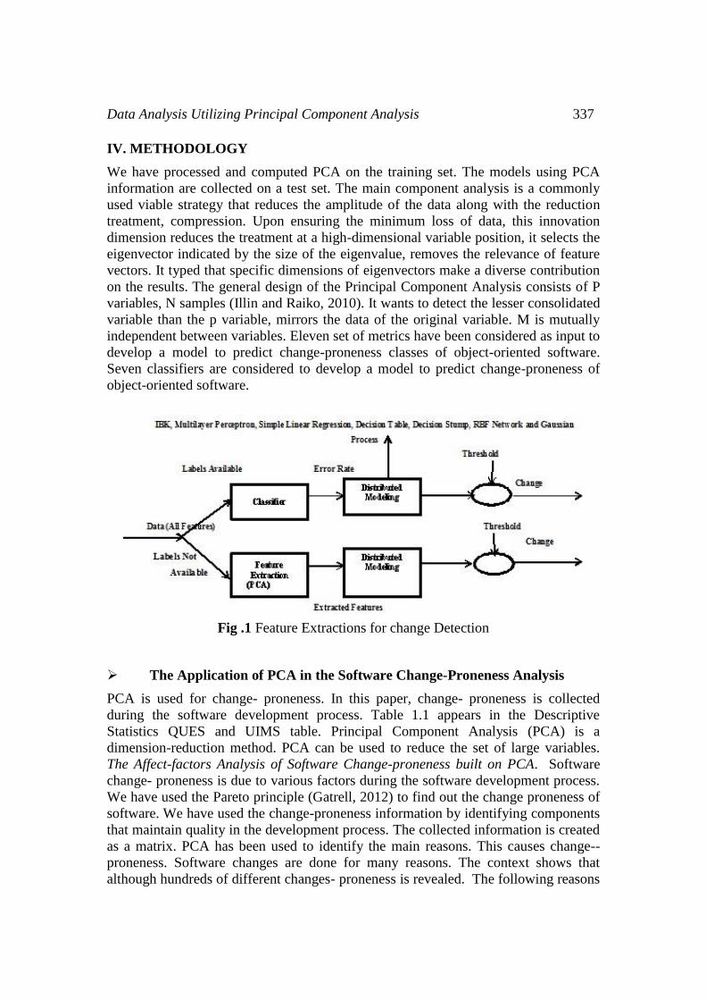
Seven classifiers are considered to develop a model to predict change-proneness of
object-oriented software.
Fig .1 Feature Extractions for change Detection
The Application of PCA in the Software Change-Proneness Analysis
PCA is used for change- proneness. In this paper, change- proneness is collected
during the software development process. Table 1.1 appears in the Descriptive
Statistics QUES and UIMS table. Principal Component Analysis (PCA) is a
dimension-reduction method. PCA can be used to reduce the set of large variables.
The Affect-factors Analysis of Software Change-proneness built on PCA. Software
change- proneness is due to various factors during the software development process.
We have used the Pareto principle (Gatrell, 2012) to find out the change proneness of
software. We have used the change-proneness information by identifying components
that maintain quality in the development process. The collected information is created
as a matrix. PCA has been used to identify the main reasons. This causes change--
proneness. Software changes are done for many reasons. The context shows that
although hundreds of different changes- proneness is revealed. The following reasons
338 Bhawana Mathur, Manju Kaushik
(at least one) are followed in software: inadequate or mistaken specification(IES);
confusion of client communication(MCC); deliberate deviation from
specification(IDS); infringement of programming standards(VPS); error in data
representation(EDR); inconsistent module interface(IMI); error in design 10gic(EDL);
incomplete or erroneous testing(IET); erroneous or deficient documentation(IID);
error in programming language translation of design(PLT); equivocal or conflicting
human-computer interface(HCI); others(OTS).
V. DATA ANALYSIS AND VERIFICATION
The principal component analysis is a multi-dimensional analysis technique. Analysis
of the relations between certain components has been done. With the help of PCA and
machine learning technology, changes-proneness in UIMS and QUES software are
calculated by changes-proneness and performance measurements. The software
focuses on the key factors that make changes. With huge datasets, the test became
more accurate and in this way, it increased the productivity process after increasing
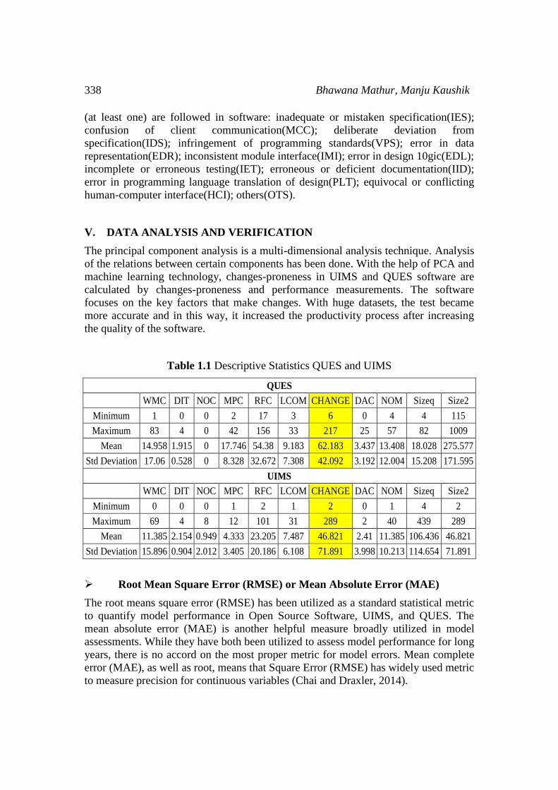
the quality of the software.
Table 1.1 Descriptive Statistics QUES and UIMS
QUES
WMC DIT NOC MPC RFC LCOM CHANGE DAC NOM Sizeq Size2
Minimum 1 0 0 2 17 3 6 0 4 4 115
Maximum 83 4 0 42 156 33 217 25 57 82 1009
Mean 14.958 1.915 0 17.746 54.38 9.183 62.183 3.437 13.408 18.028 275.577
Std Deviation 17.06 0.528 0 8.328 32.672 7.308 42.092 3.192 12.004 15.208 171.595
UIMS
WMC DIT NOC MPC RFC LCOM CHANGE DAC NOM Sizeq Size2
Minimum 0 0 0 1 2 1 2 0 1 4 2
Maximum 69 4 8 12 101 31 289 2 40 439 289
Mean 11.385 2.154 0.949 4.333 23.205 7.487 46.821 2.41 11.385 106.436 46.821
Std Deviation 15.896 0.904 2.012 3.405 20.186 6.108 71.891 3.998 10.213 114.654 71.891
Root Mean Square Error (RMSE) or Mean Absolute Error (MAE)
The root means square error (RMSE) has been utilized as a standard statistical metric
to quantify model performance in Open Source Software, UIMS, and QUES. The
mean absolute error (MAE) is another helpful measure broadly utilized in model
assessments. While they have both been utilized to assess model performance for long
years, there is no accord on the most proper metric for model errors. Mean complete
error (MAE), as well as root, means that Square Error (RMSE) has widely used metric
to measure precision for continuous variables (Chai and Draxler, 2014).
Data Analysis Utilizing Principal Component Analysis 339
PCA
A common use of PCA is to reduce the dimensions of the dataset. The following six
steps have been followed:
1) The covariance matrix of the original D-dimensional dataset X is calculated.
2) The eigenvectors as well as the covariance matrix calculate the eigenvalues.
3) Sorted eigenvalues by reducing the request.
4) Select k eigenvectors which is the number of new feature dimensions where
the subspace is compared to the largest eigenvalues.
5) Selected eigenvectors matrix projection matrix w is produced.
6) To get Dimensional Feature SubSpace Y, first changed the Dataset X.
The proportion of eigenvalues is the proportion of illustrative significance of the
factors as for the variables. If a factor has a low eigenvalue, at that point it is
contributing little to the clarification of variances in the variables and might be
disregarded as repetitive with more imperative factors. Eigenvalues measure the
amount of variety in the total sample represented by each factor. A factor's eigenvalue
might be processed as the entirety of its squared factor loadings for all the variables.
Note that the eigenvalues related with the unrotated and rotated solution will vary;
however, their aggregate will be the same. The key component is to check the
eigenvalues for decision making.
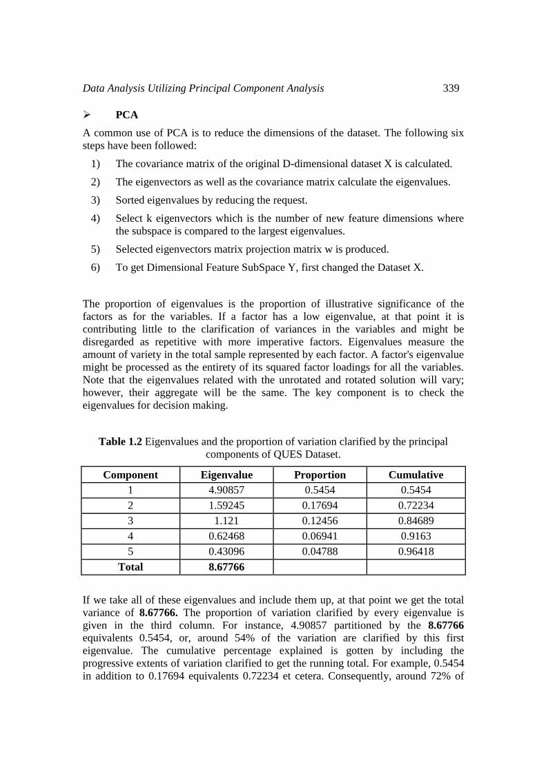
Table 1.2 Eigenvalues and the proportion of variation clarified by the principal
components of QUES Dataset.
Component Eigenvalue Proportion Cumulative
1 4.90857 0.5454 0.5454
2 1.59245 0.17694 0.72234
3 1.121 0.12456 0.84689
4 0.62468 0.06941 0.9163
5 0.43096 0.04788 0.96418
Total 8.67766
If we take all of these eigenvalues and include them up, at that point we get the total
variance of 8.67766. The proportion of variation clarified by every eigenvalue is
given in the third column. For instance, 4.90857 partitioned by the 8.67766
equivalents 0.5454, or, around 54% of the variation are clarified by this first
eigenvalue. The cumulative percentage explained is gotten by including the
progressive extents of variation clarified to get the running total. For example, 0.5454
in addition to 0.17694 equivalents 0.72234 et cetera. Consequently, around 72% of
340 Bhawana Mathur, Manju Kaushik
the variation is clarified by the initial two eigenvalues together. Next, we need to take
a gander at progressive contrasts between the eigenvalues. Subtracting the second
eigenvalue 1.59245 from the first eigenvalue, 4.90857 we get a distinction of 3.31612.
The contrast between the second and third eigenvalues is 0.47145; the following
distinction is 0.49632. Consequent contrasts are significantly littler. A sharp drop
starting with one eigenvalue then onto the next may fill in as another pointer of what
number of eigenvalues to consider. The initial three principal components clarify 84%
of the variation. This is an acceptable substantial percentage.
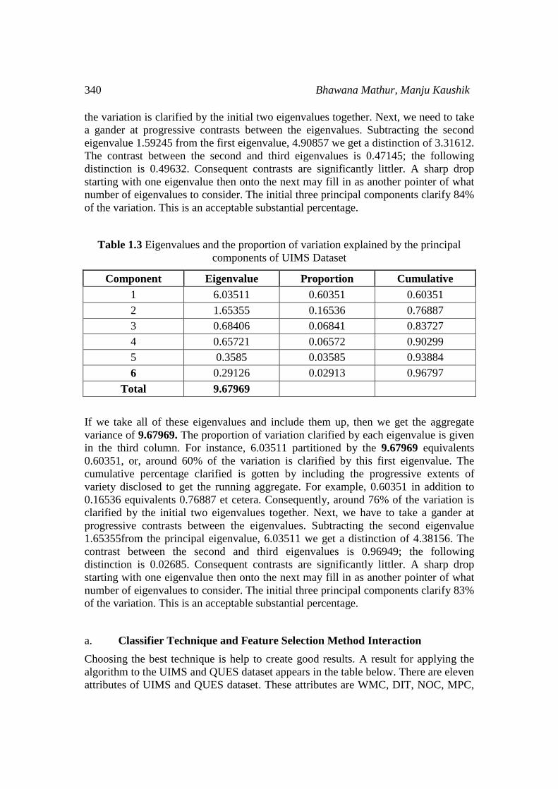
Table 1.3 Eigenvalues and the proportion of variation explained by the principal
components of UIMS Dataset
Component Eigenvalue Proportion Cumulative
1 6.03511 0.60351 0.60351
2 1.65355 0.16536 0.76887
3 0.68406 0.06841 0.83727
4 0.65721 0.06572 0.90299
5 0.3585 0.03585 0.93884
6 0.29126 0.02913 0.96797
Total 9.67969
If we take all of these eigenvalues and include them up, then we get the aggregate
variance of 9.67969. The proportion of variation clarified by each eigenvalue is given
in the third column. For instance, 6.03511 partitioned by the 9.67969 equivalents
0.60351, or, around 60% of the variation is clarified by this first eigenvalue. The
cumulative percentage clarified is gotten by including the progressive extents of
variety disclosed to get the running aggregate. For example, 0.60351 in addition to
0.16536 equivalents 0.76887 et cetera. Consequently, around 76% of the variation is
clarified by the initial two eigenvalues together. Next, we have to take a gander at
progressive contrasts between the eigenvalues. Subtracting the second eigenvalue
1.65355from the principal eigenvalue, 6.03511 we get a distinction of 4.38156. The
contrast between the second and third eigenvalues is 0.96949; the following
distinction is 0.02685. Consequent contrasts are significantly littler. A sharp drop
starting with one eigenvalue then onto the next may fill in as another pointer of what
number of eigenvalues to consider. The initial three principal components clarify 83%
of the variation. This is an acceptable substantial percentage.
a. Classifier Technique and Feature Selection Method Interaction
Choosing the best technique is help to create good results. A result for applying the
algorithm to the UIMS and QUES dataset appears in the table below. There are eleven
attributes of UIMS and QUES dataset. These attributes are WMC, DIT, NOC, MPC,
Data Analysis Utilizing Principal Component Analysis 341
RFC, LCOM, CHANGE, DAC, NOM, SIZEq, SIZE2. We are running the classifier
in Weka of specific dataset. I have seen that if I'm endeavoring to predict a nominal
value the result particularly demonstrates the accurately and incorrectly predicted
values.
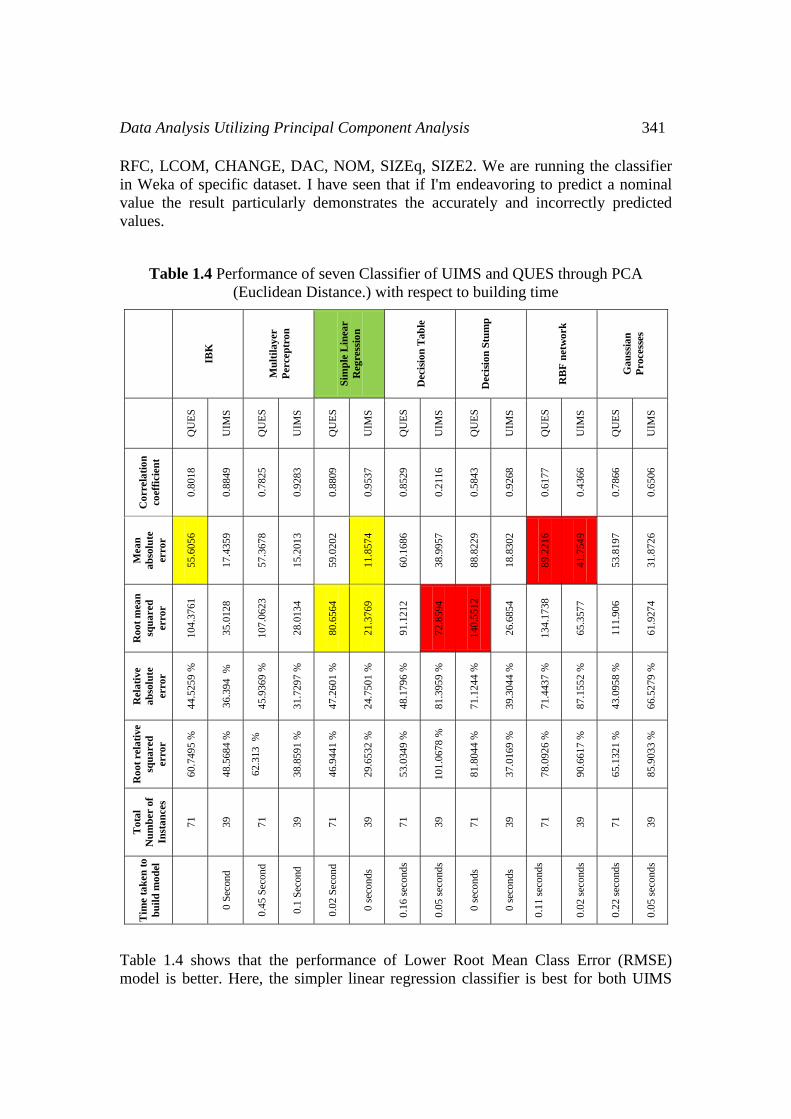
Table 1.4 Performance of seven Classifier of UIMS and QUES through PCA
(Euclidean Distance.) with respect to building time
IBK
Mu
ltil
ay
er
Perce
ptr
on
Sim
ple
Lin
ear
Reg
ress
ion
Decis
ion
Ta
ble
Decis
ion
Stu
mp
RB
F n
etw
ork
Ga
uss
ian
Process
es
QU
ES
UIM
S
QU
ES
UIM
S
QU
ES
UIM
S
QU
ES
UIM
S
QU
ES
UIM
S
QU
ES
UIM
S
QU
ES
UIM
S
Co
rre
lati
on
co
eff
icie
nt
0.8
018
0.8
849
0.7
825
0.9
283
0.8
809
0.9
537
0.8
529
0.2
116
0.5
843
0.9
268
0.6
177
0.4
366
0.7
866
0.6
506
Mea
n
ab
solu
te
erro
r
55.6
05
6
17.4
35
9
57.3
67
8
15.2
01
3
59.0
20
2
11.8
57
4
60.1
68
6
38.9
95
7
88.8
22
9
18.8
30
2
89.2
21
6
41.7
54
9
53.8
19
7
31.8
72
6
Ro
ot
mea
n
squ
ared
erro
r
104
.37
61
35.0
12
8
107
.06
23
28.0
13
4
80.6
56
4
21.3
76
9
91.1
21
2
72.8
59
4
140
.55
12
26.6
85
4
134
.17
38
65.3
57
7
111
.90
6
61.9
27
4
Rela
tive
ab
solu
te
erro
r
44.5
25
9 %
36.3
94
%
45.9
36
9 %
31.7
29
7 %
47.2
60
1 %
24.7
50
1 %
48.1
79
6 %
81.3
95
9 %
71.1
24
4 %
39.3
04
4 %
71.4
43
7 %
87.1
55
2 %
43.0
95
8 %
66.5
27
9 %
Ro
ot
rel
ati
ve
squ
ared
erro
r
60.7
49
5 %
48.5
68
4 %
62.3
13
%
38.8
59
1 %
46.9
44
1 %
29.6
53
2 %
53.0
34
9 %
101
.06
78
%
81.8
04
4 %
37.0
16
9 %
78.0
92
6 %
90.6
61
7 %
65.1
32
1 %
85.9
03
3 %
To
tal
Nu
mb
er o
f
Inst
an
ces
71
39
71
39
71
39
71
39
71
39
71
39
71
39
Tim
e t
ak
en
to
bu
ild
mo
del
0 S
econd
0.4
5 S
econ
d
0.1
Sec
ond
0.0
2 S
econ
d
0 s
eco
nd
s
0.1
6 s
econd
s
0.0
5 s
econd
s
0 s
eco
nd
s
0 s
eco
nd
s
0.1
1 s
econd
s
0.0
2 s
econd
s
0.2
2 s
econd
s
0.0
5 s
econd
s
Table 1.4 shows that the performance of Lower Root Mean Class Error (RMSE)
model is better. Here, the simpler linear regression classifier is best for both UIMS
342 Bhawana Mathur, Manju Kaushik
and QUES dataset. The main aim of Principal Component Analysis (PCA) is to
reduce the density of a dataset with diverse performances in datasets. Many variables
correlated with each other, while to the extreme degree, diversified performance in
datasets, this technique is called compression information. In Table 1.4, Simple
Linear Regression, Root Mean Square Error is lower like 21.3769, 80.6564 for UIMS
and QUES data set respectively. Therefore, Simple Linear Regression is better. Mean
absolute error is 11.8574 for UIMS Simple Linear Regression.
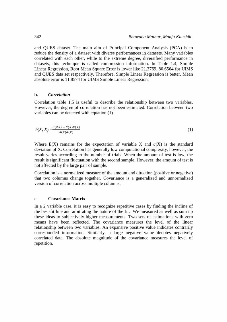
b. Correlation
Correlation table 1.5 is useful to describe the relationship between two variables.
However, the degree of correlation has not been estimated. Correlation between two
variables can be detected with equation (1).
δ(X, X) =𝐸(𝑋𝑋) − 𝐸(𝑋)𝐸(𝑋)
𝜎(𝑋)𝜎(𝑋) (1)
Where E(X) remains for the expectation of variable X and σ(X) is the standard
deviation of X. Correlation has generally low computational complexity, however, the
result varies according to the number of trials. When the amount of test is low, the
result is significant fluctuation with the second sample. However, the amount of test is
not affected by the large pair of sample.
Correlation is a normalized measure of the amount and direction (positive or negative)
that two columns change together. Covariance is a generalized and unnormalized
version of correlation across multiple columns.
c. Covariance Matrix
In a 2 variable case, it is easy to recognize repetitive cases by finding the incline of
the best-fit line and arbitrating the nature of the fit. We measured as well as sum up
these ideas to subjectively higher measurements. Two sets of estimations with zero
means have been reflected. The covariance measures the level of the linear
relationship between two variables. An expansive positive value indicates contrarily
corresponded information. Similarly, a large negative value denotes negatively
correlated data. The absolute magnitude of the covariance measures the level of
repetition.
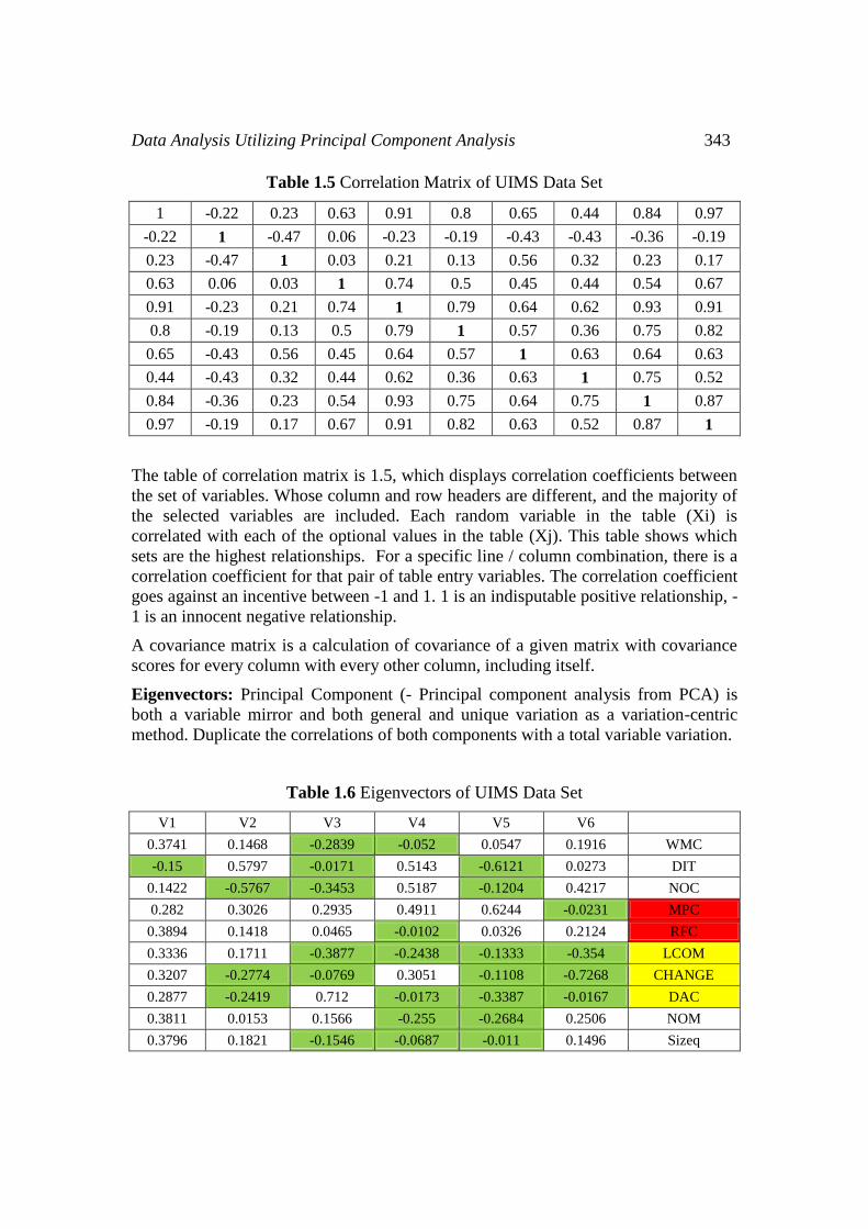
Data Analysis Utilizing Principal Component Analysis 343
Table 1.5 Correlation Matrix of UIMS Data Set
1 -0.22 0.23 0.63 0.91 0.8 0.65 0.44 0.84 0.97
-0.22 1 -0.47 0.06 -0.23 -0.19 -0.43 -0.43 -0.36 -0.19
0.23 -0.47 1 0.03 0.21 0.13 0.56 0.32 0.23 0.17
0.63 0.06 0.03 1 0.74 0.5 0.45 0.44 0.54 0.67
0.91 -0.23 0.21 0.74 1 0.79 0.64 0.62 0.93 0.91
0.8 -0.19 0.13 0.5 0.79 1 0.57 0.36 0.75 0.82
0.65 -0.43 0.56 0.45 0.64 0.57 1 0.63 0.64 0.63
0.44 -0.43 0.32 0.44 0.62 0.36 0.63 1 0.75 0.52
0.84 -0.36 0.23 0.54 0.93 0.75 0.64 0.75 1 0.87
0.97 -0.19 0.17 0.67 0.91 0.82 0.63 0.52 0.87 1
The table of correlation matrix is 1.5, which displays correlation coefficients between
the set of variables. Whose column and row headers are different, and the majority of
the selected variables are included. Each random variable in the table (Xi) is
correlated with each of the optional values in the table (Xj). This table shows which
sets are the highest relationships. For a specific line / column combination, there is a
correlation coefficient for that pair of table entry variables. The correlation coefficient
goes against an incentive between -1 and 1. 1 is an indisputable positive relationship, -
1 is an innocent negative relationship.
A covariance matrix is a calculation of covariance of a given matrix with covariance
scores for every column with every other column, including itself.
Eigenvectors: Principal Component (- Principal component analysis from PCA) is
both a variable mirror and both general and unique variation as a variation-centric
method. Duplicate the correlations of both components with a total variable variation.
Table 1.6 Eigenvectors of UIMS Data Set
V1 V2 V3 V4 V5 V6
0.3741 0.1468 -0.2839 -0.052 0.0547 0.1916 WMC
-0.15 0.5797 -0.0171 0.5143 -0.6121 0.0273 DIT
0.1422 -0.5767 -0.3453 0.5187 -0.1204 0.4217 NOC
0.282 0.3026 0.2935 0.4911 0.6244 -0.0231 MPC
0.3894 0.1418 0.0465 -0.0102 0.0326 0.2124 RFC
0.3336 0.1711 -0.3877 -0.2438 -0.1333 -0.354 LCOM
0.3207 -0.2774 -0.0769 0.3051 -0.1108 -0.7268 CHANGE
0.2877 -0.2419 0.712 -0.0173 -0.3387 -0.0167 DAC
0.3811 0.0153 0.1566 -0.255 -0.2684 0.2506 NOM
0.3796 0.1821 -0.1546 -0.0687 -0.011 0.1496 Sizeq
344 Bhawana Mathur, Manju Kaushik
Variation-Covariance matrix is designed as a component of eigenvalues and their
comparative eigenvectors. Eigenvectors are very similar. Each eigenvector resembles
a skewer helps put linear transformation. Usually at that point, a linear mapping is a
measure of contortion stimulated by the transformation. The eigenvectors inform
about distortion oriented.
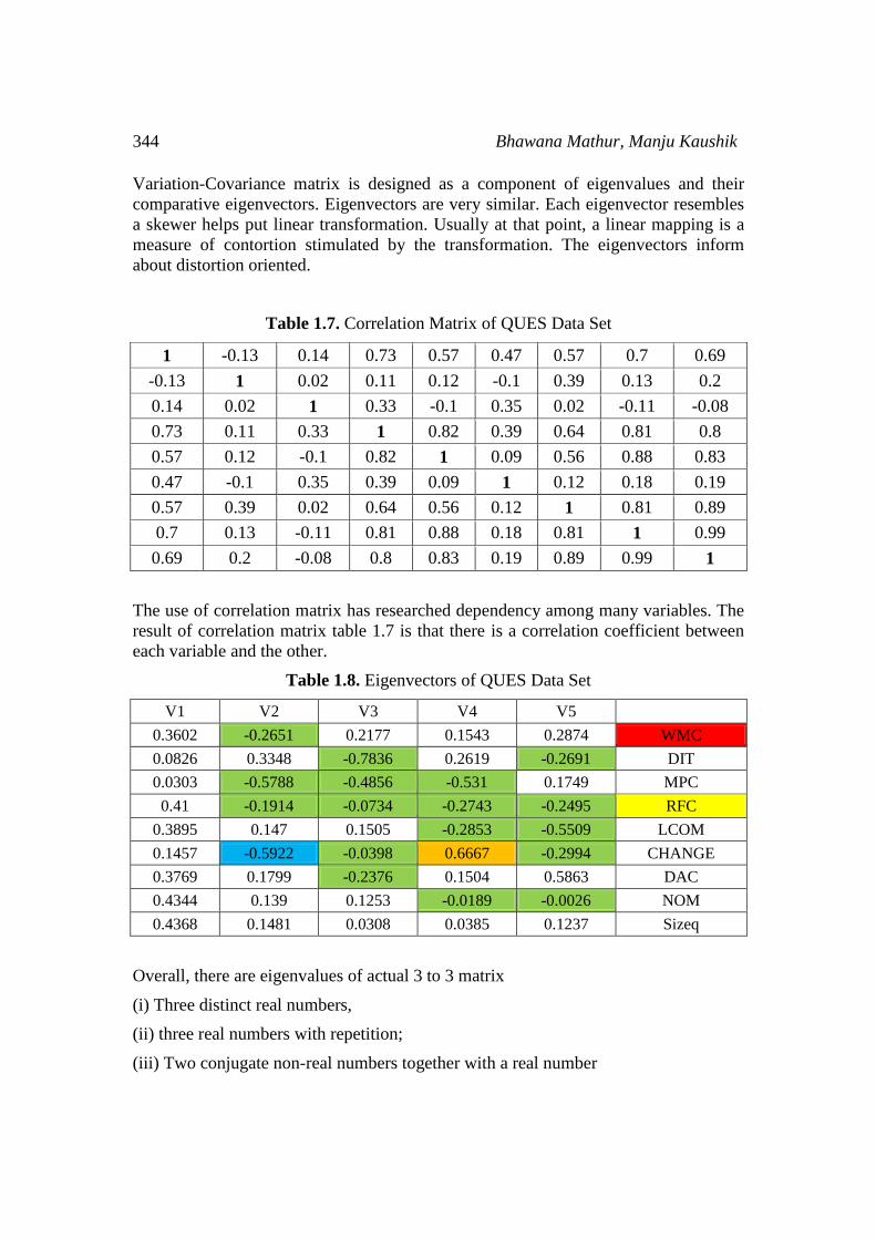
Table 1.7. Correlation Matrix of QUES Data Set
1 -0.13 0.14 0.73 0.57 0.47 0.57 0.7 0.69
-0.13 1 0.02 0.11 0.12 -0.1 0.39 0.13 0.2
0.14 0.02 1 0.33 -0.1 0.35 0.02 -0.11 -0.08
0.73 0.11 0.33 1 0.82 0.39 0.64 0.81 0.8
0.57 0.12 -0.1 0.82 1 0.09 0.56 0.88 0.83
0.47 -0.1 0.35 0.39 0.09 1 0.12 0.18 0.19
0.57 0.39 0.02 0.64 0.56 0.12 1 0.81 0.89
0.7 0.13 -0.11 0.81 0.88 0.18 0.81 1 0.99
0.69 0.2 -0.08 0.8 0.83 0.19 0.89 0.99 1
The use of correlation matrix has researched dependency among many variables. The
result of correlation matrix table 1.7 is that there is a correlation coefficient between
each variable and the other.
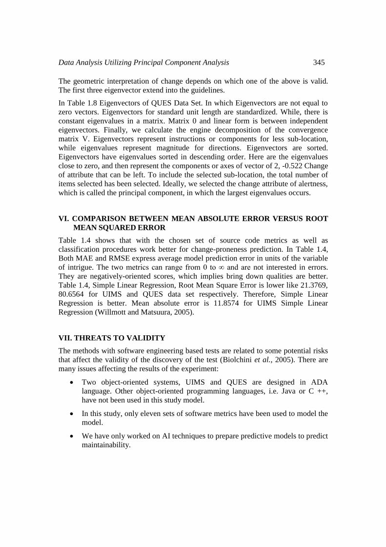
Table 1.8. Eigenvectors of QUES Data Set
V1 V2 V3 V4 V5
0.3602 -0.2651 0.2177 0.1543 0.2874 WMC
0.0826 0.3348 -0.7836 0.2619 -0.2691 DIT
0.0303 -0.5788 -0.4856 -0.531 0.1749 MPC
0.41 -0.1914 -0.0734 -0.2743 -0.2495 RFC
0.3895 0.147 0.1505 -0.2853 -0.5509 LCOM
0.1457 -0.5922 -0.0398 0.6667 -0.2994 CHANGE
0.3769 0.1799 -0.2376 0.1504 0.5863 DAC
0.4344 0.139 0.1253 -0.0189 -0.0026 NOM
0.4368 0.1481 0.0308 0.0385 0.1237 Sizeq
Overall, there are eigenvalues of actual 3 to 3 matrix
(i) Three distinct real numbers,
(ii) three real numbers with repetition;
(iii) Two conjugate non-real numbers together with a real number
Data Analysis Utilizing Principal Component Analysis 345
The geometric interpretation of change depends on which one of the above is valid.
The first three eigenvector extend into the guidelines.
In Table 1.8 Eigenvectors of QUES Data Set. In which Eigenvectors are not equal to
zero vectors. Eigenvectors for standard unit length are standardized. While, there is
constant eigenvalues in a matrix. Matrix 0 and linear form is between independent
eigenvectors. Finally, we calculate the engine decomposition of the convergence
matrix V. Eigenvectors represent instructions or components for less sub-location,
while eigenvalues represent magnitude for directions. Eigenvectors are sorted. Eigenvectors have eigenvalues sorted in descending order. Here are the eigenvalues
close to zero, and then represent the components or axes of vector of 2, -0.522 Change
of attribute that can be left. To include the selected sub-location, the total number of
items selected has been selected. Ideally, we selected the change attribute of alertness,
which is called the principal component, in which the largest eigenvalues occurs.
VI. COMPARISON BETWEEN MEAN ABSOLUTE ERROR VERSUS ROOT
MEAN SQUARED ERROR
Table 1.4 shows that with the chosen set of source code metrics as well as
classification procedures work better for change-proneness prediction. In Table 1.4,
Both MAE and RMSE express average model prediction error in units of the variable
of intrigue. The two metrics can range from 0 to ∞ and are not interested in errors.
They are negatively-oriented scores, which implies bring down qualities are better. Table 1.4, Simple Linear Regression, Root Mean Square Error is lower like 21.3769,
80.6564 for UIMS and QUES data set respectively. Therefore, Simple Linear
Regression is better. Mean absolute error is 11.8574 for UIMS Simple Linear
Regression (Willmott and Matsuura, 2005).
VII. THREATS TO VALIDITY
The methods with software engineering based tests are related to some potential risks
that affect the validity of the discovery of the test (Biolchini et al., 2005). There are
many issues affecting the results of the experiment:
Two object-oriented systems, UIMS and QUES are designed in ADA
language. Other object-oriented programming languages, i.e. Java or C ++,
have not been used in this study model.
In this study, only eleven sets of software metrics have been used to model the
model.
We have only worked on AI techniques to prepare predictive models to predict
maintainability.
346 Bhawana Mathur, Manju Kaushik
VIII. RESULT AND DISCUSSION
Simple Linear Regression, Root Mean Square Error is lower like 21.3769, 80.6564 for
UIMS and QUES data set respectively. Therefore, Simple Linear Regression is better.
Mean absolute error is 11.8574 for UIMS Simple Linear Regression. Square roots are
sometimes used with full values. The basis of this is that when using the roots of the
class, there is a greater effect on the results of extreme values. Mean Absolute error
(MAE) with both root mean square errors (RMSE), has often been used in model
evaluation studies. Root means Squire Error (RMSE) has been used as a standard
statistical metric for measuring model performance in open source software, UIMS
and QUES.
IX. CONCLUSION AND FUTURE SCOPE
The software that generates change- proneness rates and increases the quality of the
software. By examining information about change- proneness, we find that there is
some change in the software development process. After the change-proneness
process, the update software delivered to the customer. For the purpose of displaying
feature extraction, we were only interested in an acceptable recognition of change in
the middle. There are various uses of PCA that will be used for the upcoming
predictions of using the Weka as well as statistical packages for Social Sciences
(SPSS) software. Apart from this, we can extend the work to reduce the facility by
using feature reduction techniques, i.e. PCA, RST, statistical tests etc.
REFERENCE
[1] Biolchini, J., Mian, P.G., Natali, A.C.C. and Travassos, G.H., 2005.
Systematic review in software engineering. System Engineering and Computer
Science Department COPPE/UFRJ, Technical Report ES, 679(05), p.45.
[2] Chai, T. and Draxler, R.R., 2014. Root mean square error (RMSE) or mean
absolute error (MAE)?–Arguments against avoiding RMSE in the
literature. Geoscientific model development, 7(3), pp.1247-1250.
[3] Chen, J.C. and Huang, S.J., 2009. An empirical analysis of the impact of
software development problem factors on software maintainability. Journal of
Systems and Software, 82(6), pp.981-992.
[4] Ernst, N.A., 2012. Software Evolution: a Requirements Engineering
Approach (Doctoral dissertation, University of Toronto (Canada)).
[5] Guo, Y., 2016. Measuring and monitoring technical debt. University of
Maryland, Baltimore County.
[6] Gatrell, M., 2012. An empirical investigation into contributory factors of
change and fault propensity in large-scale commercial object-oriented
software (Doctoral dissertation, Brunel University, School of Information
Systems, Computing and Mathematics).
Data Analysis Utilizing Principal Component Analysis 347
[7] Han, A.R., Jeon, S.U., Bae, D.H. and Hong, J.E., 2010. Measuring behavioral
dependency for improving change-proneness prediction in UML-based design
models. Journal of Systems and Software, 83(2), pp.222-234.
[8] Jayatilleke, S. and Lai, R., 2017. A systematic review of requirements change
management. Information and Software Technology.
[9] Ilin, A. and Raiko, T., 2010. Practical approaches to principal component
analysis in the presence of missing values. Journal of Machine Learning
Research, 11(Jul), pp.1957-2000. [10] Kafura, D. and Henry, S., 1981.
Software quality metrics based on interconnectivity. Journal of Systems and
Software, 2(2), pp.121-131.
[11] Koru, A.G. and Liu, H., 2007. Identifying and characterizing change-prone
classes in two large-scale open-source products. Journal of Systems and
Software, 80(1), pp.63-73.
[12] Kumar, L., Behera, R.K., Rath, S. and Sureka, A., 2017. Transfer Learning for
Cross-Project Change-Proneness Prediction in Object-Oriented Software
Systems: A Feasibility Analysis. ACM SIGSOFT Software Engineering
Notes, 42(3), pp.1-11.
[13] Kumar, L., Rath, S. and Sureka, A., 2017, July. An empirical analysis on
effective fault prediction model developed using ensemble methods.
In Computer Software and Applications Conference (COMPSAC), 2017 IEEE
41st Annual (Vol. 1, pp. 244-249). IEEE. [14] Kumar, L., Rath, S.K. and
Sureka, A., 2017, February. Empirical analysis on effectiveness of source code
metrics for predicting change-proneness. In Proceedings of the 10th
Innovations in Software Engineering Conference (pp. 4-14). ACM.
[15] Kumar, L., Rath, S.K. and Sureka, A., 2017, February. Using source code
metrics to predict change-prone web services: A case-study on ebay services.
In Machine Learning Techniques for Software Quality Evaluation
(MaLTeSQuE), IEEE Workshop on (pp. 1-7). IEEE.
[16] Kumar, L. and Sureka, A., 2017, February. Using structured text source code
metrics and artificial neural networks to predict change proneness at code tab
and program organization level. In Proceedings of the 10th Innovations in
Software Engineering Conference (pp. 172-180). ACM.
[17] Kumar, L. and Sureka, A., 2017. A Comparative Study of Different Source
Code Metrics and Machine Learning Algorithms for Predicting Change
Proneness of Object Oriented Systems. arXiv preprint arXiv:1712.07944.
[18] Li, W. and Henry, S., 1993, May. Maintenance metrics for the object oriented
paradigm. In Software Metrics Symposium, 1993. Proceedings., First
International (pp. 52-60). IEEE.
[19] Lu, H., Zhou, Y., Xu, B., Leung, H. and Chen, L., 2012. The ability of object-
oriented metrics to predict change-proneness: a meta-analysis. Empirical
software engineering, 17(3), pp.200-242.
348 Bhawana Mathur, Manju Kaushik
[20] Malhotra, R. and Chug, A., 2016. Software Maintainability: Systematic
Literature Review and Current Trends. International Journal of Software
Engineering and Knowledge Engineering, 26(08), pp.1221-1253.
[21] Sharafat, A.R. and Tahvildari, L., 2008. Change prediction in object-oriented
software systems: A probabilistic approach. Journal of Software, 3(5), pp.26-
39.
[22] Willmott, C.J. and Matsuura, K., 2005. Advantages of the mean absolute error
(MAE) over the root mean square error (RMSE) in assessing average model
performance. Climate research, 30(1), pp.79-82.
[23] Witten, I.H., Frank, E., Hall, M.A. and Pal, C.J., 2016. Data Mining: Practical
machine learning tools and techniques. Morgan Kaufmann.
[24] Zhou, Y. and Leung, H., 2007. Predicting object-oriented software
maintainability using multivariate adaptive regression splines. Journal of
Systems and Software, 80(8), pp.1349-1361.