Embed Size (px)
Citation preview

Data Appendix for "Industry performance and indirect access to structural holes," Page �
Data appenDiXfor "Industry Performance and Indirect Access to Structural Holes," Ronald S. Burt
(2008) in Advances in Strategic Management, edited by Joel A. C. Baum and Timothy J. Rowley. New York: Elsevier. Work cited here can be found in the chapter
references, except for Burt (�998), which is a research report available on my research website under the title "Partitioning the American economy for organization research."
network DataNetwork data used in the chapter are available as NetDraw files from my research website (www.chicagogsb.edu/fac/ronald.burt/research). File "iotable87.txt" contains the �987 input-output data. File "iotable92.txt" contains the �992 data. After you download the files, change the .txt extentions to .vna, then load the files in NetDraw. Each file contains non-zero buying and selling among the 403 industries distinguished in the analysis (56,763 relations in �987, 43,472 in �987). Nodes are presented in the NetDraw files with an input-output ID, the four categories of concentration distinguished in Figure 4 of the chapter, a concentration score, a direct network constraint score, and a short industry name. Relations are listed as dyads: producer industry, other industry, the percentage of producer business done with the other, and dollars of business with the other (in millions).
performance DataFigure A�, at the top of the next page, shows that relative industry performance in �987 continued by and large into �992, but margins were slightly higher on average in �987, and a few industries operated at a loss in one or the other year. No industry operated at a loss in both years. Beginning with the four negative price-cost margins in �987 (to the left in Figure A�), the most extreme is in ‘Miscellaneous Ordnance and Accessories.’ The Department of Commerce distinguished six input-output categories in the armaments industry. Five of the six were about as profitable in �992 as they were in �987 (missiles, tanks, small arms, small-arms ammunition, and ammunition other than small-arms). The residual category, ‘Miscellaneous Ordnance and Accessories,’ was a small industry of about a billion and a half dollars producing assorted tactical weapons such as artillery, flame throwers, rocket launchers, etc. ($�.6 billion in �987, $�.3 billion in �992). The industry was highly concentrated and Honeywell was the leading producer (77% four-firm concentration ratio in �987, 83% in �992). Miscalculations following the collapse of the Iron Curtain resulted in large losses for Honeywell’s operations in the industry. In �990, the operations were spun off as Alliant Techsystems, and put on a more solid footing. In �987, however, the large Honeywell losses summed into the industry operating at an extreme loss indicated in Figure A�. Switching to the five negative price-cost margins

Data Appendix for "Industry performance and indirect access to structural holes," Page 2
in �992, ‘Primary Nonferrous Metals’ ran the largest loss. The former Iron Curtain was again an issue. When the Soviet Union collapsed, Russian smelters who had served the Soviet military dumped their low-priced aluminum on the world market, triggering a severe drop in the market price for aluminum from American producers. Given that the nine negative price-cost margins are year specific (each is positive in the other panel), and would have disproportionate influence on estimated effects because they are at the extreme edge of the data distributions, I put the nine aside as intrusive outliers. This turns out not to affect conclusions about the statistical significance of effects, but it does make effects stand out more clearly since the nine temporary outliers do not have to be fit into the aggregate performance associations with industry structure. As quick illustration, here are estimates for the baseline model (Eq. 3) fit across all 722 observations of the 36� manufacturing industries, including adjustment for the slightly higher margins in �987:
PCM = 4�.37 – 4.07 ln (�00-O) – 3.99 ln (C) + 2.45 D87, (�.48) (.8�) (.4�)where standard errors are given in parentheses (adjusted for autocorrelation across repeated observations using the ‘cluster’ option in STATA). There is a statistically significant
Figure a1price-Cost Margins in the two Benchmark Years
-0.2
0.0
0.2
0.4
0.6
0.8
-0.2 0.0 0.2 0.4 0.6 0.8
Pri
ce-C
ost
Mar
gin
in 1
992
Price-Cost Margin in 1987
PCM92 =
.025 + .725 PCM87
Misc. Ordnanceand Accessories
130700
380501Primary Nonferrous Metals

Data Appendix for "Industry performance and indirect access to structural holes," Page 3
-2.75 t-test for the negative effect of producer rivalry, and a -4.92 t-test for the negative effect of supplier-customer network constraint. Here are estimates fit across all 640 observations of the 320 industries that correspond to unique four-digit SIC categories:
PCM = 42.3� – 4.�4 ln (�00-O) – 4.�8 ln (C) + 2.5� D87, (�.52) (.87) (.4�)which define t-tests of -2.70 and -4.8� respectively for producer rivalry and network constraint. And here are estimates for the baseline model fit across the further subset of 632 observations in which price-cost margins were nonnegative (eight of the nine negative margins occur in the more-narrowly defined, and so more subject to exogenous shock, industries that correspond to unique four-digit SIC categories):
PCM = 48.4� – 5.42 ln(�00-O) – 4.39 ln(C) + 2.38 D87, (�.4�) (.80) (.4�)which define t-tests of -3.83 and -5.47 respectively for producer rivalry and network constraint. Three points are illustrated: First, the two industry-structure effects are, as expected, negative and statistically significant. Second, estimates do not differ much between the equation estimated across all 36� manufacturing industries and the one estimated across the 320 manufacturing industries that correspond to unique four-digit SIC categories. Third, effects are more clear — stronger magnitudes and smaller standard errors — in the equation for which I put aside the nine negative price-cost margins as temporary outliers. I tested alternative treatments. I estimated effects with the nine outliers included as routine data, with the nine truncated to a value of zero profit, with a dummy variable distinguishing the outliers, and with the nine outliers simply put aside to be explained on a case by case basis. I get the same results with the different treatments except industry-structure effects are slightly more clear with the nine outliers excluded or distinguished by a dummy variable since the model does not have to fit them into the aggregate performance associations with industry structure. I put the nine outliers aside rather than add an ‘outlier’ dummy variable to the network model to preserve the simplicity of the network model and because the dummy variable would be a temporary complication peculiar to the years observed here.
network Model VariablesRaw and log scores on the variables used to generate the main results in Tables � and 2 of the chapter are available in an Excel file (main.xls) and a STATA file (main.dta) from my research website. The two data files contain scores for all 722 observations of the

Data Appendix for "Industry performance and indirect access to structural holes," Page 4
36� manufacturing industries (an observation of the industry in �987, and another in �992). Estimates in the chapter are based on the 632 nonnegative price-cost margins in the 320 manufacturing industries that correspond to a unique four-digit SIC category (NSIC = � and PCM > 0). The data should generate the means, standard deviations, and correlations in the above table. Here are the variables in the files (log scores in the files are the same names preceded by the letter "l"):
YR - year in which the industry was observed (87 or 92) IOID - industry's six-digit input-output table identification code NSIC - number of four-digit SIC categories contained in the input-output industry NDIR - number direct supplier-customer industries over the 2% business criterion NINDIR - number indirect supplier-customer industries over the 2% criterion PCM - price-cost margin for the industry D87 - dummy variable equal to � for observations in �987 O - industry concentration score C - direct network constraint on industry (Eq. 4 in chapter) IC� - unweighted indirect network constraint on industry IC2 - weighted average indirect network constraint on industry IC3 - percent industry business with low-constraint supplier-customer industries IC4 - percent industry business with high-constraint supplier-customer industries
Table A1: Means, Standard Deviations,
and Correlations for Predictions in Table 1 of the Chapter.
.33
.78
-.64
.84
1.00.38-.12-.05-.24.372.25
-.04
-.04
.03
-.04
.01
.01
1.00.12.50.50
1.00.41-.53.45.62-.04-.23.291.02
1.00-.57.82.34-.13-.211.531.63
3.70
2.17
2.52
3.99
16.89
Mean
.80
.48
.55
.50
9.46
S.D.
1.00
-.51
.40
1.00
-.77
1.00
.15
-.19
-.06
1.00
1.00.23
-.19
-.24
-.27
IC1: Unweighted Average C
1987
IC5: Extended Network C
IC4: Percent High-C
IC2: Weighted Average C
Log(C)
IC3: Percent Low-C
Log(100-O)
PCM
Note — These results are computed across nonnegative price-cost margins in the 320 manufacturing industries corresponding to unique
four-digit SIC categories in 1987 and 1992 (N = 632). All variables, except price-cost margins (PCM) and the dummy variable
distinguishing observations in 1987, are measured as log scores. Criterion to be a supplier-customer is 2% of industry business.
Log(100-O) measures the constraint of rivalry between producers in an industry (O is the four-firm concentration ratio). Log(C) measures
the network constraint of dependence on concentrated supplier-customer industries (Eq. 4 in the chapter). Indirect network constraint
measures are discussed in the text around Table 1 in the chapter.

Data Appendix for "Industry performance and indirect access to structural holes," Page 5
IC5 - total network constraint across indirect supplier-customer industries TAB2 - four-category network variable in Table 2 of the chapter NAME - input-output industry name
Bounding the immediate networkThe above data are based on a 2% criterion defining the boundary of an industry's immediate network. Estimating spillover effects requires a criterion distinguishing the end of one network and the beginning of another. Competitive advantage can then be assessed for the extent to which it spills over across adjacent boundaries. In theory, the immediate network consists of a producer industry plus every other industry with which it has business. How much business qualifies? For the �992 benchmark input-output table, the Department of Commerce rounded dollar flows to the nearest million dollars. If a million dollars is the criterion in the 403-industry table, then the immediate network around an average manufacturing industry would contain 87.2 other industries as suppliers or customers, varying from a minimum of �6 to a maximum of 375. In the �987 input-output table, dollar flows are rounded to the nearest $�00,000. The �987 table contains more non-zero dollar flows (56,763 among the 403 industries versus 43,472 in the �992 table). The difference between the tables is almost entirely small dollar flows in �987 that would not round up to a million dollars for the �992 table (�3,742 dollar flows in the �987 table are .5 million or less). Using the $�00,000 minimum dollar flow as a criterion, the immediate network around an average manufacturing industry would contain �22.3 other industries as suppliers or customers, varying from a minimum of 23 to a maximum of 400, which is almost every one of the other 402 industries in the table. I prefer not to use “any business” as the criterion for inclusion in the immediate network around an industry. There would be inconsistency between the �987 and �992 tables, and immediate networks would be large, leaving little of the economy for the extended network. Large networks in a small population produce extended networks that regress to the population mean since each extended network quickly includes every node in the population (see Burt, 2007a:�45-�46, for illustration in a population of investment bankers). Table A2 at the top of the next page shows how industry network size would vary with five alternative boundary criteria: any buying or selling with the industry, �% of industry buying and selling, 2%, 5%, and �0%. Criteria are expressed as percentages of producer buying and selling as is usual in studies of resource dependence. Dollar amounts large for one industry can be trivial for another. Table A2 shows that the primary difference between �987 and �992 is in the small transactions and that even a small limit on what qualifies as business brings network size

Data Appendix for "Industry performance and indirect access to structural holes," Page 6
13
12
6.50
6.29
2
2
66.8%
66.2%
1987
1992
Three Percent of
Producer Business
40.7%
40.4%
56.7%
56.3%
73.9%
73.5%
84.3%
82.1%
100.0%
100.0%
Average
Percent of
Business in
the Network
5
4
1.71
1.73
0
0
1987
1992
Ten Percent of
Producer Business
8
8
3.97
3.85
1
1
1987
1992
Five Percent of
Producer Business
19
17
9.30
9.18
2
3
1987
1992
Two Percent of
Producer Business
34
31
16.56
16.90
4
4
1987
1992
One Percent of
Producer Business
399
375
121.34
86.31
24
17
1987
1992
Any Producer
Buying or Selling
Largest
Network
Average
Network
Smallest
NetworkYear
Criterion for
Inclusion in the
Immediate
Network around
Producer Industry
Network Size
Table A2: Defining the Immediate Network.
Note — These are counts for the 361 manufacturing industries. Percent of business in the network is the sum of pij that
exceed the criterion, where pij is the percentage of producer buying and selling transacted with industry j. Each of the
other 402 input-output sectors is a potential supplier or customer. Producer industry is not included in the counts.
down to a practical number of supplier and customer markets that a manager could be expected to monitor. If immediate networks are limited to industries with which producers conduct at least one percent of their buying and selling, the immediate networks around manufacturing industries in �987 average �6.6 other industries as suppliers or customers, varying from a minimum of 4, up to a maximum of 34. Network size is about the same in �992. Increasing the criterion to two percent cuts network size in half; averages of 9.3 and 8.8 respectively in �987 and �992. Increasing the criterion to five percent halves the networks once again to reach average sizes of 4.2 and 4.� in �987 and �992. Business is clearly concentrated in a few key supplier and customer industries, with smaller but substantial amounts of business conducted in other industries. The substantial amounts are indicated in Table A2 by the percent of business included in the networks. Even a low criterion of one percent excludes from the industry networks �7% of producer business on average (84.3% of producer business in �987 is included in the one-percent networks, 82.�% of business in �992). To cast a broad network, my instinct was to use a one-percent criterion. Networks would be a manageable size and roughly similar in �987 and �992, while retaining a high level of producer business. However,

Data Appendix for "Industry performance and indirect access to structural holes," Page 7
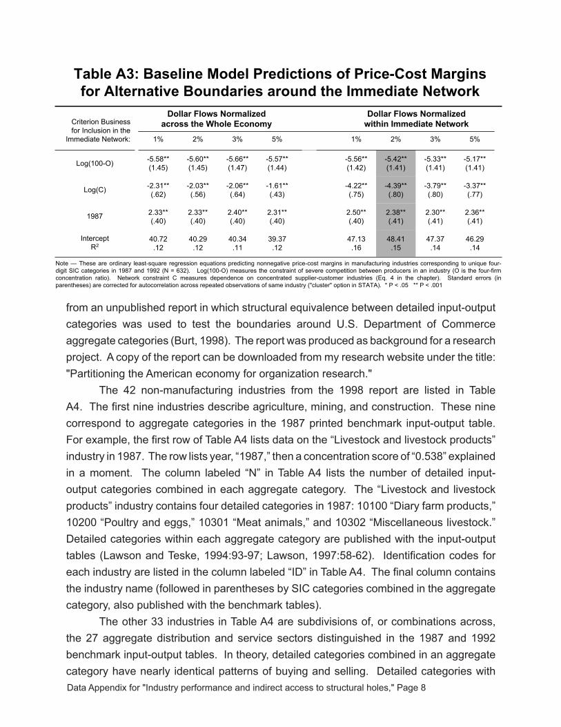
it is not clear that all those small one-percent transactions need to be included in the network. Given the lack of a clear criterion for the immediate network around an industry, I estimated effects in the baseline network model for four alternative criteria — one percent, two percent, three percent, and five percent — to determine where the boundary should be drawn. The results are presented in Table A3 at the top of the next page. I draw three conclusions from the results. First, the negative effect of rivalry within the industry is stable across all the alternatives. The coefficient is consistently about negative five and a half with a standard error of about one and a half. Second, the 2% criterion seems to me to be the right criterion to define the immediate network around industries in the chapter. The results for 2% in Table A3 are about the same as the results for the more extensive �% criterion, and slightly stronger than the slightly more restrictive criteria of 3% and 5%. Given substantial producer business excluded from the networks by a two-percent criterion (about a quarter of producer business on average), I tested for industry differences in the amount of business excluded, and report in footnote 8 to the chapter that controlling for the percent of producer business included in an industry's network adds nothing to the Table � predictions. Third, after defining the boundary of a network, I normalize connections to the relative proportion of business transacted within the network. The four models to the left in Table A3 use the raw pij defined in Eq. (5) in the chapter. The raw pij measure the proportion of all industry i buying and selling that is transacted with industry j. In other words, the pij are normalized — they sum to one — across all production industries in the economy. The four models to the right in Table A3 use pij normalized within the immediate network around an industry: pij = pij / Sk pik, i ≠ j, where the sum is across all industries k in the immediate network excluding industry i itself. This assumes that the connections most relevant to the focal industry are the connections within its immediate network, not connections across the economy. Normalizing within the immediate network is exactly what is done with manager networks defined by survey network data, so I am comfortable using the same operationalization with industry networks to obtain stronger network effects. The final result is that the shaded column in Table A3 is the baseline network model in the chapter.
Data on non-ManufacturingAggregation is not an actionable issue for the manufacturing industries in the chapter because I use the most detailed input-output categories available. Non-manufacturing categories and a measure of producer organization within the categories were taken
Data Appendix for "Industry performance and indirect access to structural holes," Page 8
from an unpublished report in which structural equivalence between detailed input-output categories was used to test the boundaries around U.S. Department of Commerce aggregate categories (Burt, �998). The report was produced as background for a research project. A copy of the report can be downloaded from my research website under the title: "Partitioning the American economy for organization research." The 42 non-manufacturing industries from the �998 report are listed in Table A4. The first nine industries describe agriculture, mining, and construction. These nine correspond to aggregate categories in the �987 printed benchmark input-output table. For example, the first row of Table A4 lists data on the “Livestock and livestock products” industry in �987. The row lists year, “�987,” then a concentration score of “0.538” explained in a moment. The column labeled “N” in Table A4 lists the number of detailed input-output categories combined in each aggregate category. The “Livestock and livestock products” industry contains four detailed categories in �987: �0�00 “Diary farm products,” �0200 “Poultry and eggs,” �030� “Meat animals,” and �0302 “Miscellaneous livestock.” Detailed categories within each aggregate category are published with the input-output tables (Lawson and Teske, �994:93-97; Lawson, �997:58-62). Identification codes for each industry are listed in the column labeled “ID” in Table A4. The final column contains the industry name (followed in parentheses by SIC categories combined in the aggregate category, also published with the benchmark tables). The other 33 industries in Table A4 are subdivisions of, or combinations across, the 27 aggregate distribution and service sectors distinguished in the �987 and �992 benchmark input-output tables. In theory, detailed categories combined in an aggregate category have nearly identical patterns of buying and selling. Detailed categories with
Table A3: Baseline Model Predictions of Price-Cost Margins
for Alternative Boundaries around the Immediate Network
47.37
.14
2.30**
(.41)
-3.79**
(.80)
-5.33**
(1.41)
3%
40.34
.11
2.40**
(.40)
-2.06**
(.64)
-5.66**
(1.47)
3%
46.29
.14
2.36**
(.41)
-3.37**
(.77)
-5.17**
(1.41)
5%
48.41
.15
2.38**
(.41)
-4.39**
(.80)
-5.42**
(1.41)
2%
39.37
.12
2.31**
(.40)
-1.61**
(.43)
-5.57**
(1.44)
5%
40.29
.12
2.33**
(.40)
-2.03**
(.56)
-5.60**
(1.45)
2%
47.13
.16
40.72
.12
2.50**
(.40)
2.33**
(.40)
-4.22**
(.75)
-5.56**
(1.42)
1%
-2.31**
(.62)
-5.58**
(1.45)
1%
1987
Intercept
R2
Log(C)
Log(100-O)
Criterion Business
for Inclusion in the
Immediate Network:
Dollar Flows Normalized
within Immediate Network
Dollar Flows Normalized
across the Whole Economy
Note — These are ordinary least-square regression equations predicting nonnegative price-cost margins in manufacturing industries corresponding to unique four-
digit SIC categories in 1987 and 1992 (N = 632). Log(100-O) measures the constraint of severe competition between producers in an industry (O is the four-firm
concentration ratio). Network constraint C measures dependence on concentrated supplier-customer industries (Eq. 4 in the chapter). Standard errors (in
parentheses) are corrected for autocorrelation across repeated observations of same industry ("cluster" option in STATA). * P < .05 ** P < .001

Data Appendix for "Industry performance and indirect access to structural holes," Page 9
similar patterns of buying and selling are “structurally equivalent” in network terminology. Where the structural equivalence analysis of buying and selling among detailed categories revealed segregated clusters within an aggregate category, I divided the aggregate category down to separate categories for the different clusters. The Department of Commerce distinguished 77 aggregate categories in the benchmark input-output tables just before the �987 table, then 88 aggregate categories in the �987 and �992 benchmark tables. The 88 aggregate categories were revised to �23 in the structural equivalence analysis. The revised industry categories have more reliable boundaries and higher construct validity (Burt, �998): Structural equivalence within industry categories increases across the three partitions (65.7% on average for the 77 categories, 70.�% for the 88 categories, 78.4% for the �23 categories). Variation in price-cost margins is increasingly between, rather than within, industries across the three partitions (48.9% between industries for the 77 categories, 49.8% between for the 88 categories, 7�.�% between for the �23 categories). The ID codes in Table A4 show where Department of Commerce categories were expanded. Identification codes follow the convention used by the Department of Commerce, and are the codes with which non-manufacturing industries are identified in the distributed data (iotable87.vna, iotable92.vna, main.xls, main.dta). The initial two digits are the industry ID in the Department of Commerce 77-category partition. For example, “65” is the transportation industry. A capital letter following a digit indicates an industry expanded from the 77-category partition. For example, the transportation industry was expanded by the Department of Commerce for the �987 benchmark input-output table to distinguish five industries: railroads (65A), trucking and warehousing (65B), water transportation (65C), air transportation (65D), and a residual category of pipelines, freight forwarders, and travel agents (65E). Where there is no capital letter following the digit, the category continued unchanged from the initial 77-category partition. For example, industry 67 continued to be radio and TV broadcasting. Finally, a lower-case letter at the end of an ID number in Table A4 marks an industry expanded from the 88-category partition. For example, the residual transportation category contained a pipeline industry (65Eb) with a pattern of buying and selling distinct from the pattern for freight forwarders and travel agents (65Ea). I tried three measures of concentration in non-manufacturing. For each, I computed a network constraint variable based on four-firm concentration in the manufacturing industries and a concentration approximation in the 42 non-manufacturing industries, then estimated a network constraint effect in the baseline network model (Eq. 3 in the chapter). The first alternative was approximations based on company size distributions as used in previous research and described in the chapter text. These data yield the estimates reported in the chapter for the baseline network model (shaded model in Table A3), reproduced here as a reference point:

Data Appendix for "Industry performance and indirect access to structural holes," Page �0
PCM = 48.4� - 5.42 Log (�00-O) - 4.39 Log (C) + 2.38 D87, (�.4�) (.80) (.4�)which generates a squared multiple correlation of .�5, a -3.83 t-test for the negative effect of rivalry within the industry, and a -5.47 t-test for network constraint from industry suppliers and customers. Second, I tried computing network constraint under the assumption that non-manufacturing industries (farming, mining, construction, services, and distribution) were so full of competitors such that concentration could be treated as zero. I get the following estimates for the baseline model:
PCM = 48.4� - 5.42 Log (�00-O) - 4.39 Log (C) + 2.38 D87, (�.4�) (.80) (.4�)which generates a squared multiple correlation of .09, a -3.4� t-test for the negative effect of rivalry within the industry, and a negligible -�.2� t-test for network constraint. Third, I tried an approximation more sophisticated than the one based on company size. The unpublished report provides a measure of producer organization in �987 and �992 (Burt, �998:Table 3) from which I derived scores in non-manufacturing analogous to the concentration ratios in manufacturing. “Effective organization” (EO) was introduced to measure how well competition within an industry, as competition affected profits, was captured for organization research by traditional concentration data (Burt, et al. 2002). EO scores are obtained by reversing the baseline network model. Instead of predicting price-cost margins from O and C as measures of industry structure, the observed price-cost in an industry and its dependence weights on other sectors are held constant (i.e., the data provided by an input-output table are held constant), and producer concentration in each industry is obtain numerically so as to align observed profit margins with the level expected from industry structure. In industries where margins are higher than expected, producers are “effectively” more organized than they appear to be. Such industries tend to be regional markets (versus national) or subject to government regulation (Burt et al., 2002). For example, there are numerous hotels operating in the United States, but only one down the street from your business, so your local hotel can enjoy profits higher than would be expected from the number of hotels operating nationally. In industries where margins are lower than expected from observed industry structure, producers are “effectively” less organized than they appear to be, which is primarily correlated with imports increasing the level of competition within an industry above the level implied by concentration among American producers (Burt et al., 2002). Using EO scores to approximate concentration in non-manufacturing, I get the following estimates for the baseline model:*
PCM = 46.78 - 5.�6 Log (�00-O) - 3.26 Log (C) + 2.�9 D87, (�.47) (�.�3) (.40)

Data Appendix for "Industry performance and indirect access to structural holes," Page ��
which generates a squared multiple correlation of .��, a -3.50 t-test for the negative effect of rivalry within the industry, and a -2.89 t-test for network constraint from industry suppliers and customers. The network constraint effect is significantly negative, but weaker than the effect estimated with size-based approximations, so I returned to the size-based approximations in the chapter and report them in Table A4 in the column labelled "O."
*The one change I made to the EO scores was to adjust them to a metric comparable to the four-firm concentration ratios in manufacturing. EO scores average .55� in �987, and .535 in �992, across the 80 aggregate manufacturing industries distinguished in Burt (�998). Four-firm concentration ratios average .395 in �987, and .405 in �992, across the 36� detailed manufacturing industries analyzed in this chapter. To convert the non-manufacturing EO scores in Burt (�998:Table 3) to a scale comparable to the manufacturing four-firm concentration ratios used in the chapter, EO scores in non-manufacturing were multiplied by .7�7 in �987 and .757 in �992 (mean EO in manufacturing divided by mean four-firm con-centration in manufacturing).

Data Appendix for "Industry performance and indirect access to structural holes," Page �2
tabl
e a
4: a
ggre
gate
non
-Man
ufac
turin
g in
dust
ries
iD � 2 3 4 5-6 7 8
9-�0
��-�
2
65A
65B
65C
65D
65E
a
65E
b
agg
rega
te in
put-O
utpu
t ind
ustr
y (S
iC c
odes
)
Live
stoc
k &
live
stoc
k pr
oduc
ts (*
0�9,
025
�-3,
02�
�-4,
*02
�9, 0
24, *
0259
, 027
�-3,
*02
79, *
029)
Oth
er a
gric
ultu
ral p
rodu
cts
(0��
, 0�3
, 0�6
, 0�7
, 0�8
, *0�
9, *
02�9
, *02
59, *
029)
Fore
stry
& fi
sher
y pr
oduc
ts (0
8�, 0
83, 0
97, 0
9�)
Agr
icul
tura
l, fo
rest
ry, &
fish
ery
serv
ices
(025
4, *
0279
, 07�
-2,0
75-6
, 078
, 085
, 092
)
Met
allic
ore
s m
inin
g (ir
on, c
oppe
r & o
ther
; �0�
-4, �
06, *
�08,
�09
4, �
099)
Coa
l min
ing
(�22
-3, *
�24)
Cru
de p
etro
leum
& n
atur
al g
as (�
3�-2
, *�3
8)
Non
met
allic
min
eral
s m
inin
g (�
4�-2
, �44
, �45
, �47
, *�4
8, �
49)
Con
stru
ctio
n (�
5, �
6, �
7, *
�08,
*�2
4, *
�38,
*�4
8, *
6552
)
Rai
lroad
s &
rela
ted
serv
ices
(40,
4�, 4
74)
Mot
or fr
eigh
t tra
nspo
rtatio
n &
war
ehou
sing
(42�
-3)
W
ater
tran
spor
tatio
n (4
4)
A
ir tra
nspo
rtatio
n (4
5)
†
Frei
ght f
orw
arde
rs &
trav
el a
gent
s (4
72-3
, 478
)
†
Pip
lines
(exc
ept n
atur
al g
as; 4
6)
Year
�987
�992
�987
�992
�987
�992
�987
�992
�987
�992
�987
�992
�987
�992
�987
�992
�987
�992
�987
�992
�987
�992
�987
�992
�987
�992
�987
�992
�987
�992
n 4 4 �3 �3 2 2 2 2 3 3 � � � � 5 5 5 �5 2 2 � 2 � � � � 2 2 � �
O
0.53
80.
627
0.63
90.
667
0.62
60.
667
0.36
90.
560
0.4�
70.
303
0.62
00.
690
0.68
�0.
700
0.58
00.
584
0.27
20.
239
0.34
70.
375
0.34
20.
3�2
0.�7
30.
345
0.33
50.
328
0.40
80.
496
0.69
40.
740

Data Appendix for "Industry performance and indirect access to structural holes," Page �3
agg
rega
te in
put-O
utpu
t ind
ustr
y (S
iC c
odes
)
Com
mun
icat
ion
(exc
ept r
adio
& T
V; 4
8�-2
, 484
, 489
)
Rad
io &
TV
bro
adca
stin
g (4
83)
Ele
ctric
ser
vice
s (u
tiliti
es; 4
9�, 4
93�)
G
as p
rodu
ctio
n &
dis
tribu
tion
(util
ities
; 492
2-5,
493
2, 4
939)
W
ater
& s
anita
ry s
ervi
ces
(494
, 495
2-3,
495
9, 4
96-7
)
Who
lesa
le tr
ade(
50, 5
�)
R
etai
l tra
de(5
2-7,
59)
Fina
nce
(60,
6�,
62,
67,
exc
ludi
ng 6
732)
†
Insu
ranc
e ca
rrie
rs (6
3)
† In
sura
nce
agen
ts (6
4)
Ow
ner-
occu
pied
dw
ellin
gs (—
)
†
Rea
l est
ate
agen
ts (6
5, e
xclu
ding
655
2)
† R
oyal
ties
(—)
Hot
els
& lo
dgin
g pl
aces
(70�
-4)
P
erso
nal &
repa
ir se
rvic
es (e
xcep
t aut
o; 7
2�-6
, 729
, 762
-4)
tabl
e a
4: a
ggre
gate
non
-Man
ufac
turin
g in
dust
ries,
con
tinue
d
iD 66 67 68A
68B
68C
69A
69B
70A
70B
a
70B
b
7�A
7�B
a
7�B
b
72A
72B
n � 2 � � � � � 2 2 2 � � � � 3 3 � � � � � � � � � � � 2 6 6
O
0.52
50.
58�
0.52
20.
646
0.58
20.
632
0.57
70.
664
0.00
70.
475
0.39
50.
406
0.49
90.
592
0.30
�0.
5�6
0.47
70.
548
0.66
30.
703
0.70
40.
747
0.64
40.
680
0.7�
70.
757
0.4�
�0.
475
0.40
20.
5�8
Year
�987
�992
�987
�992
�987
�992
�987
�992
�987
�992
�987
�992
�987
�992
�987
�992
�987
�992
�987
�992
�987
�992
�987
�992
�987
�992
�987
�992
�987
�992

Data Appendix for "Industry performance and indirect access to structural holes," Page �4
tabl
e a
4: a
ggre
gate
non
-Man
ufac
turin
g in
dust
ries,
con
tinue
d
Agg
rega
te In
put-O
utpu
t Ind
ustry
(SIC
cod
es)
Com
pute
r & d
ata
proc
essi
ng s
ervi
ces
(737
)
†
Lega
l ser
vice
s (8
�)
† E
ngin
eerin
g se
rvic
es (8
7�)
† M
anag
emen
t, ac
coun
ting,
& te
stin
g se
rvic
es (8
72, 8
73, 8
74, 8
9)
† G
ener
al b
usin
ess
serv
ices
(733
�, 7
32, 7
334,
733
8, 7
34-6
, 738
�-3,
738
9, 7
69)
† P
hoto
grap
hic
serv
ices
(733
5-6,
738
4)
Adv
ertis
ing
serv
ices
(73�
)
E
atin
g &
drin
king
pla
ces
(58)
Aut
omot
ive
repa
ir &
ser
vice
s (7
5�-3
, 754
2, 7
549)
Am
usem
ents
(78�
-4, 7
9�-3
, 794
�, 7
948,
799
�-3,
799
6-7,
799
9)
Hea
lth s
ervi
ces
(074
, 80�
-3, 8
04�-
3, 8
049,
805
-6, 8
07-9
)
Edu
catio
nal &
soc
ial s
ervi
ces
(673
2, 8
2�-4
, 829
, 832
-3, 8
35-6
, 839
, 84,
86�
-6, 8
69, 8
733)
Year
�987
�992
�987
�992
�987
�992
�987
�992
�987
�992
�987
�992
�987
�992
�987
�992
�987
�992
�987
�992
�987
�992
�987
�992
O
0.38
80.
467
0.46
60.
542
0.44
90.
529
0.�9
70.
483
0.46
20.
567
0.50
70.
647
0.42
50.
526
0.33
90.
4�2
0.44
60.
49�
0.4�
90.
547
0.34
20.
453
0.22
30.
408
N � � � � � � 2 3 6 6 � � � � � � 3 3 8 8 4 6 �� ��
ID 73A
73B
a
73B
b
73B
C
73C
a
73C
b
73D
74 75 76 77A
77B
Not
e —
Dat
a ar
e ex
plai
ned
in th
e te
xt.
Ast
eris
k in
dica
tes
that
par
tial S
IC c
ateg
ory
is in
the
row
indu
stry
. D
agge
r (†)
indi
cate
s a
row
indu
stry
dis
aggr
egat
ed
from
a b
road
er in
put-o
utpu
t cat
egor
y.