Data as Ensembles of Records: Representation and Comparison

Nicholas R. Howe nihowe@cs.cornell.edu

Department of Computer Science, Cornell University, Ithaca, NY 14853

Abstract

Many collections of data do not come pack-aged in a form amenable to the ready applica-tion of machine learning techniques. Never-theless, there has been only limited researchon the problem of preparing raw data forlearning, perhaps because widespread differ-ences between domains make generalizationdifficult. This paper focuses on one com-mon class of raw data, in which the enti-ties of interest actually comprise collectionsof (smaller pieces of) homologous data. Wepresent a technique for processing such col-lections into high-dimensional vectors, suit-able for the application of many learn-ing algorithms including clustering, nearest-neighbors, and boosting. We demonstratethe abilities of the method by using it to im-plement similarity metrics on two differentdomains: natural images and measurementsfrom ocean buoys in the Pacific.

1. Introduction

A quick perusal of the UCI repository of machinelearning data sets (Blake & Merz, 1999) reveals thatthe most frequently cited entries consist of data thatare condensed into a convenient format easily digestedby most machine learning algorithms. Typically suchdata consist of a set of instances, perhaps already di-vided into subsets for training and testing. Each in-dividual instance is described by a set of features X ,including a class feature that the learning algorithmmust predict accurately.

Although the data sets in the UCI repository providea convenient testbed for new ideas in machine learn-ing, they do not fully represent the difficulty of solv-ing problems encountered in the real world. Often thehardest part of applying learning methods to a previ-ously unexamined task is the codification of the prob-lem in a form that machine learning algorithms canhandle. This step has already been performed on mostof the repository data, and usually there is no accessto the original form of the data set or documentationon how it was transformed. Thus there is need for re-

search and discussion on the analysis of data in a morenatural format.

Some types of raw data may not even be amenable toexpression in the standard feature-value format, andtherefore require special treatment. For example, sometasks involve learning properties of entities that arethemselves made up of an arbitrary number of similarcomponents. As a concrete example, consider inves-tigating properties of credit accounts, where each ac-count is represented as the set of transactions postedto the account. This paper focuses on such collec-tive entities, or ensembles, in particular when the con-stituent components, or records, happen to have a con-cise featural description. Instead of devising featuresthat summarize the ensemble as a whole, which can ob-scure useful information, we adopt a description thatpreserves important details of each individual record.The algorithm presented in this paper automaticallygenerates a feature vector of uniform size from anyensemble, provided that the component records havea standard feature-vector description. This providesa novel way to look at data from many domains, in-cluding computer event logs, transactional data suchas credit card histories, and other areas where ensem-ble data are involved. We present insight from imple-mentations of the technique in two different domains:natural images and ocean measurements.

This work is far from the first to look at descriptionsof data other than the canonical feature-value repre-sentation. Researchers in case-based reasoning oftenadopt complex or unusual case descriptions (Kolod-ner, 1993). For example, Branting (1991) looks at legalcases represented as graphs. Additionally, the field ofreinforcement learning may be thought of as employingdata in a nonstandard format (Kaelbling et al., 1996).While dealing with nonstandard data representations,these fields have not focused on the type of ensembledata examined here.

The remainder of this paper describes our treatmentof ensemble data. Section 2 gives a description of thealgorithms for processing and comparing data ensem-bles. Section 3 presents the two test domains and ex-amines the performance of the system on them. Fi-nally, Section 4 concludes with a discussion of possibledirections for future research.

2. Handling Ensemble Data

We address domains in which the task requires learn-ing properties of ensembles of records, where each en-semble may contain an arbitrary number of records.Furthermore, we assume that each record is describedby a simple feature vector. To be precise, we will givea formal description of such an ensemble before de-scribing how it is processed.

A record is an arbitrary set of m feature-valuepairs, r = {(x1, y1), (x2, y2), ..., (xm, ym)}, where X ={x1, x2, ..., xm} is a consistent set of features shared byall records in the data, and the yj are values of thosefeatures. (In some domains, features may be missingfrom some records, and thus the features of r forma subset Xr ⊆ X .) An ensemble is simply a collec-tion (possibly a weighted collection) of records, i.e., aset of ordered pairs {(r1, w1), (r2, w2), . . . , (rne , wne)}where ri is a record and wi ∈ R+ is a positive realweight. As a concrete example, in a credit card do-main each ensemble might represent one account. Itscomponent records would be the charges posted tothe account, each described by a feature set, suchas {amount, charge date, payment date}. Some ac-counts would have fewer charges posted than others.

2.1 Data Preparation

Processing of ensemble data into a more manageableform takes place in two steps. First, we express theindividual records in a discrete space M, which is adiscretization of the original feature space. Once thisis done, a one-to-one function transforms the entireensemble into a vector in a high-dimensional space F .Vectors in this space may be thought of as joint his-tograms of the original record feature values. All sub-sequent processing takes place in F , which is bettersuited to the application of standard machine learningtechniques.

Records are mapped into space M by discretizing eachfeature xj . Points in M are tuples of the discretizedfeature values. Thus, to map a record to a point m inM we simply determine the appropriate bin for eachof its feature values. For the credit card example justdescribed, a hypothetical record might map to a pointlike ($50-100,Jun99,Oct99). The discretization of fea-ture value for the results reported in this paper hasbeen done by hand, but automated techniques existand might be applied (Fayyad & Irani, 1993).

Ensembles are represented as a set of ordered pairs,each consisting of a point in M and an associated posi-tive weight. (Weights arise naturally in some domains,or can be set uniformly to one if not needed. If two ormore records are described by the same m, they arerepresented by a single ordered pair with weight equalto the sum of the individual weights.) We refer to this

as the M-representation RM(e) of the ensemble e.

RM(e) = {(m1, w1), (m2, w2), ..., (mne , wne)} (1)

where ne is the number of records in the ensemble, andwi ∈ R+ is a weight.

Space F has exactly one dimension corresponding toeach point of space M. Thus F is equivalent to R

NF+ ,

where the dimensionality NF is the product of thenumber of bins used for all the features X . For ex-ample, in the simple credit account domain describedabove, there might be ten bins for the amount feature,and 20 each for the two date features, giving F a totalof 10 · 20 · 20 = 4000 dimensions. Each of these dimen-sions represents a particular range of values for trans-action amount, charge date, and payment date. Weestablish a one-to-one correspondance between pointsin M and the standard orthonormal basis vectors ofF . Thus there exists a bijective mapping f betweenM-representations and vectors in F .

f (RM(e)) =ne∑i=1

wiF (mi) (2)

where F (m) is the mapping from points in M to basisvectors of F . This means that ensembles with uniqueM-representations also have a unique representationin F .

2.2 An Example

A concrete example may illustrate the creation ofF -representations. Suppose that an account in thecredit-card domain has the following transactionsposted (ignoring interest charges for simplicity):

Date ActionJune 16, 1999 Charge $75September 2, 1999 Charge $20September 28, 1999 Charge $35October 13, 1999 Paid $130

An M-representation for this account would be

{(($50-100,Jun99,Oct99),1),(($0-50,Sep99,Oct99),2)}.

This corresponds to the F -vector

e($50−100 ,Jun99 ,Oct99 ) +2e($0−50 ,Sep99 ,Oct99 )

where e(amount,charge date,payment date) is the basis vec-tor in one of the dimensions of F , as described by thesubscript.

2.3 Vector Comparisons

In many applications, the significant information re-sides in the distribution of he records in M spacerather than the actual number of records. If this is so,

then the natural distance metric to use is the cosinemetric, which measures the angular deviation betweentwo vectors and ignores their length. The cosine met-ric has been extensively used for text retrieval (Salton,1989). Thus in F space, the distance between two vec-tors f1 and f2 is

DF(f1, f2) = cos−1

(f1 · f2√

(f1 · f1)(f2 · f2)

)(3)

While the plain cosine difference metric may work wellin some situations, a number of considerations suggestthe use of a slightly more complicated form than Equa-tion 3. If continuous variables are discretized to formM space, then their relative ordering is lost. Even fordiscrete variables, some pairs of values indicate greatersimilarity than others. We would like to capture thisinformation in the ensemble distance metric, and cando so by modifying Equation 3 to include a similaritymatrix with cross terms:

DF(f1, f2) = cos−1

fT

1 Sf2√(fT1 Sf1

) (fT2 Sf2

) . (4)

Here S is a matrix whose off-diagonal entries accountfor the varying similarity of different feature values.It should be a symmetric matrix so that distances aresymmetric, and can be devised to have a Cholesky fac-torization S = TT T. Under these conditions, Equa-tion 4 can also be interpreted as the simple cosine dif-ference between two transformed vectors Tf1 and Tf2.

The choice of S will greatly affect distance measure-ments and therefore any results based upon them. Wedescribe the system that we have used for generatingsuitable matrices, but numerous alternative possibil-ities also exist. Our approach has the advantage ofallowing the user significant control over how much in-dividual features contribute to the final distance, with-out an overly complex interface.

We form T (and hence S) as the Kronecker prod-uct (or direct matrix product) of smaller matrices{T1,T2, ...,Tm}, each corresponding to one of the fea-tures xj . Each entry in the Kronecker product matrixis the product of exactly one entry from each of theKronecker factor matrices. Intuitively, this representsthe cross terms in T, corresponding to the match be-tween two points in M (or components in F), as theproduct of the cross terms of the Tj matrices, eachrepresenting the match in one individual feature. Thususing the Kronecker product allows us to focus on onefeature at a time, and also allows for significant com-putational efficiencies as explained in Section 2.4.

Each Tj is a square matrix of a size equal to the num-ber of bins in the discretization of xj . For features thatwere originally continuous, we use cross terms that de-cay exponentially with the distance between the bincenters:

Tj(k, l) = (pj)∆j(y′k,y′

l). (5)

Here ∆j(y′k, y′

l) is the distance between the centers ofbins k and l, and pj ∈ [0, 1] is a parameter that con-trols the size of the cross terms. If pj = 0, then onlyexact matches are allowed, while pj = 1 means thatany value of feature xj matches all others equally well.Intermediate values of pj result in better matches forcloser values. Thus the setting of pj is a knob by whichthe user can exert control over the system. Althoughneither of the example data sets we examine in Sec-tion 3 contain discrete features, Tj matrices for dis-crete features can be created via an analogous pro-cess, by using something like the value-difference met-ric (Stanfill & Waltz, 1986).

2.4 Practical Concerns

Scalability is a valid concern in the system so far out-lined, but perhaps not as large a concern as might atfirst appear. Clearly, restraint must be used in dis-cretizing features, since the dimensionality of F is theproduct of the number of bins in each feature. Never-theless, the technique scales sufficiently for the analysisof interesting problems, as the experiments of Section 3demonstrate. Here we explain a few key optimizationsthat make operations in F more feasible.

The slowest calculation to perform in a straightforwardmanner is multiplication by S. Normally this would bean N2

F operation, where NF is the dimensionality ofF . However, by using S that is a Kronecker product,the matrix multiplication can be computed in time lin-ear in NF (Graham, 1981). (Essentially, the resultis calculated through repeated multiplications by thesmaller Sj matrices.) Furthermore, when comparingone ensemble represented by vector f1 to many others,the product f1S need only be computed once. For fixedS the denominator in Equation 4 can be precomputed;thus the calculation of multiple cosine differences canbe quite fast. Under ideal circumstances, it amountsto one array lookup and two floating point operationsper record.

3. Implementation and Evaluation

The algorithms described in the previous section definea similarity metric on arbitrary ensembles of records.As yet we have said nothing about how to evaluate thetechnique, nor what role it might play in a completelearning system. Fortunately, similarity lies at theheart of many learning systems. Nearest-neighbor al-gorithms, clustering, retrieval, and even sophisticatedtechniques like boosting all apply naturally in a suit-able metric space, such as F . To evaluate the use-fulness of the F -representation of ensembles, we mustshow that a proposed metric promotes effective learn-ing. In particular, if entities with similar propertiestend to be mutually similar under the cosine metric,then those properties can be successfully learned. Thispaper will look at some simple similarity-based tasks

as an indication that more complex algorithms basedon similarity may also use the cosine metric success-fully. Thus the transformations described in this papercan provide the first stage of a potential learning sys-tem, packaging raw ensemble data for analysis by astandard learning algorithm.

Although it is easy to conceive of domains where dataare structured as ensembles of records, actually ac-quiring such data is more difficult. In many cases,domains that fit the ensemble paradigm are describedusing summary information, with the raw data in en-semble form not available. For example, the UCI ma-chine learning repository contains a credit screeningdomain, but information on individual accounts is con-densed into sixteen features and there is no listing oftransactions. Nevertheless, some candidate domainscan be found. We describe the application of the tech-niques described above to two tasks: image retrievalin collections of natural images, and analysis of oceanclimate measurements from the Pacific. The point ofthese evaluations is to show that machine learning canbe done under the ensemble of records paradigm. Be-cause the two domains differ significantly, each taskreveals different aspects of the approach.

3.1 Natural Images

The ideas presented in this paper were first developedas part of an effort to improve on current algorithmsfor image retrieval. In the spirit of Impressionist art,images can be viewed as collections of many smallpatches with differing color, texture, and spatial prop-erties. Visually similar images should comprise similarcollections of patches, so a means of comparing patchcollections would imply a means of comparing images.This observation motivates the current work.

To prepare an image for comparison, we first divideit into about 500 small patches using a simple localsegmentation scheme (Felzenszwalb & Huttenlocher,1998) and arbitrarily divide further any large regionsgenerated. Next we record for each patch the values ofcolor (in the Hue-Saturation-Value color space), tex-ture (as measured by a local filter), and spatial loca-tion (normalized to the image dimensions). These arediscretized to produce the M-representation of the im-age. We use 28 color bins, 21 spatial bins, and threetexture bins. Finally, after conversion to F space, wecompare the image with others using Equation 4. OurS is created as described in Section 2.3, with the spreadparameters ranging from 0.1 to 0.001. We adjusted theparameters by hand in a small pilot study, using a gra-dient descent approach.

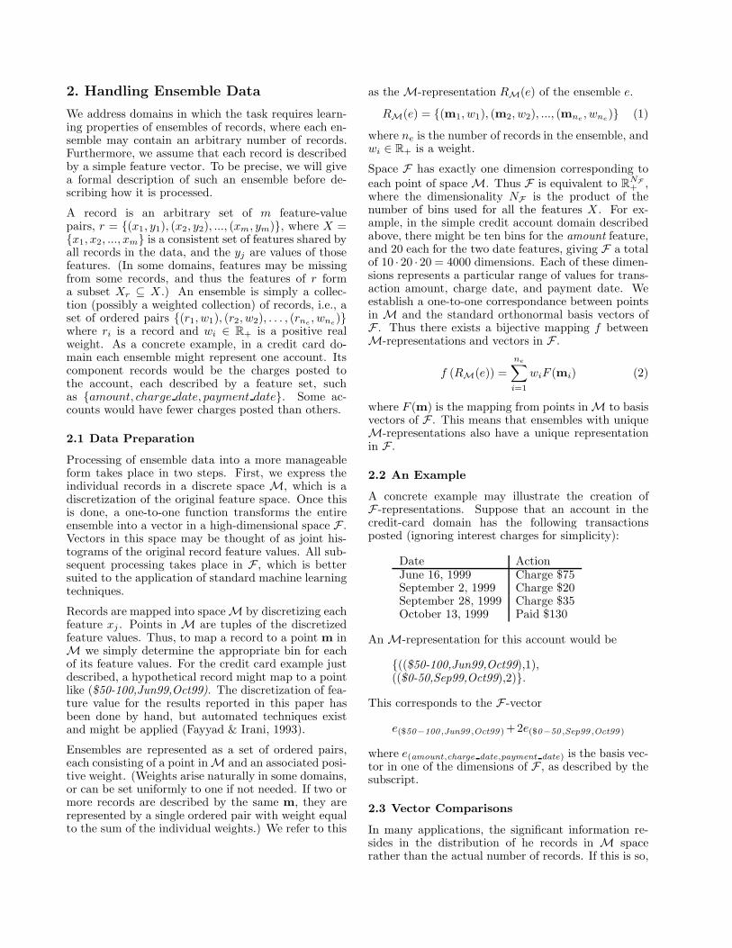
We evaluate the ensemble-based algorithm on severaltasks, in comparison with both a baseline approach(color histograms (Swain & Ballard, 1991)) and astate-of-the-art algorithm (color correlograms (Huanget al., 1997)) designed specifically for image retrieval.

Our approach does consistently better than the base-line and competes well with the specialized retrievalalgorithm.

The first test we apply uses artificially altered or de-graded images as queries, with the task of retrievingthe original from a collection of 19,000 images. (Allimages come from a commercially available collectionpublished by Corel.) The query alterations come inthree flavors: Crop, where 50% of the image area istrimmed around the borders, Jumble, where the imageis broken into 16 rectangular tiles that are reshuffledat random, and Low-Con, where the image contrast isdegraded. We test using a randomly selected sampleof 1000 query images, and record the rank at which theoriginal is retrieved. The two sets of numbers listed forthe ensemble technique represent varying conditions:the first uses a default setting for S, while the seconduses an S that is chosen to be more appropriate to thespecific task (i.e., ignoring features that are not use-ful.) The latter case simulates tasks in which domainknowledge is available a priori to guide the selectionof S.

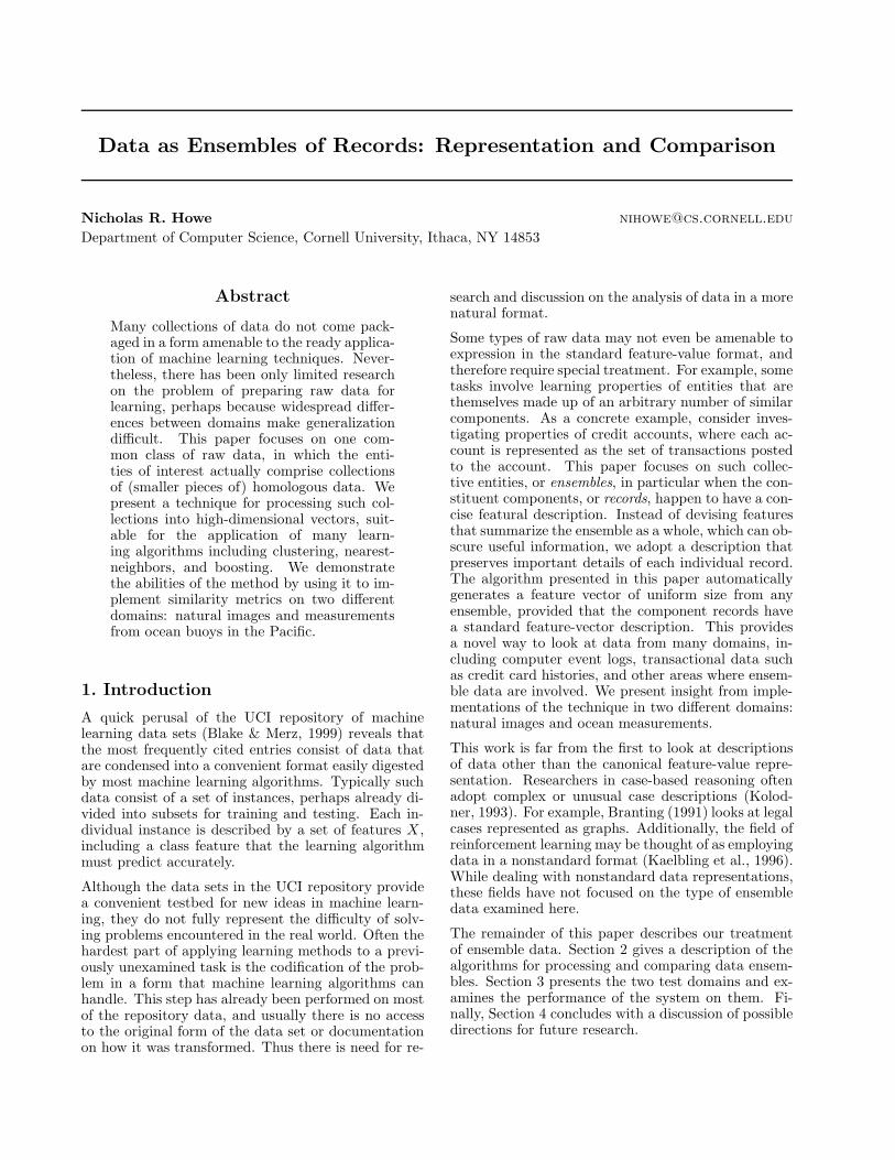
The results, in Table 1, look more or less as one mightexpect. The histogram of the ranks is quite skewedand exhibits a long tail: most originals are recoveredat a relatively low rank, but a few are not. To capturethis behavior, two numbers are listed for each con-dition. The median rank represents the bulk of thecases, while the mean rank reveals the severity of thetail. Standard deviation (σ) is also given in the table,although due to the skewed distributions it shows thesame trend as the mean.

The histogram method does worse than the others,except on the Jumble alteration, which of course doesnot affect the color histogram at all. The ensemble ap-proach with default S does worse on this task becauseunlike the other techniques it incorporates spatial fea-tures explicitly representing the position of elementsthat are moved around in this test. However, when Sis tuned to the task by smoothing out the spatial fea-ture, it does much better. The tuned ensemble methoddoes well on all three tasks.

We also look at two versions of a classification taskwhere images come from one of several visually self-similar categories. Although the category definitionsare somewhat arbitrary, this task provides some in-dication of whether using one image as a query willretrieve a related image. Because the top hits aregenerally most important for image retrieval, we fo-cus on the top images retrieved rather than thefull recall-precision curves. (The test is equivalentto one-nearest-neighbor classification under leave-one-out cross validation.) For this task we augment thepatch descriptions with an additional feature measur-ing similarity to neighboring patches in the image.This feature records whether the patch matches thecolor and texture of all, some, a few, or none of its

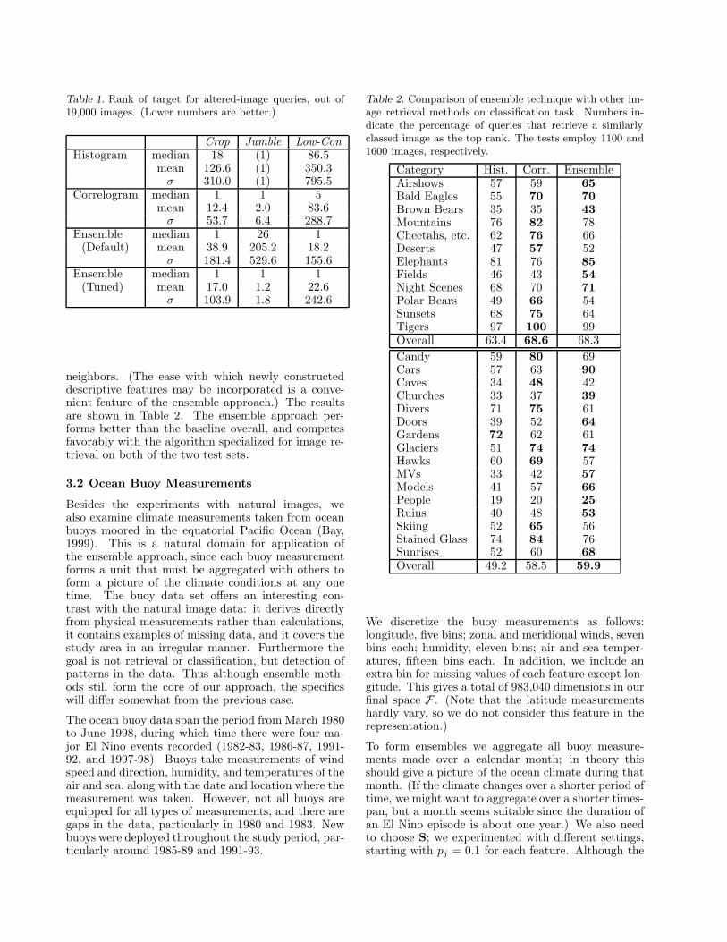
Table 1. Rank of target for altered-image queries, out of19,000 images. (Lower numbers are better.)

Crop Jumble Low-ConHistogram median 18 (1) 86.5

mean 126.6 (1) 350.3σ 310.0 (1) 795.5

Correlogram median 1 1 5mean 12.4 2.0 83.6

σ 53.7 6.4 288.7Ensemble median 1 26 1

(Default) mean 38.9 205.2 18.2σ 181.4 529.6 155.6

Ensemble median 1 1 1(Tuned) mean 17.0 1.2 22.6

σ 103.9 1.8 242.6

neighbors. (The ease with which newly constructeddescriptive features may be incorporated is a conve-nient feature of the ensemble approach.) The resultsare shown in Table 2. The ensemble approach per-forms better than the baseline overall, and competesfavorably with the algorithm specialized for image re-trieval on both of the two test sets.

3.2 Ocean Buoy Measurements

Besides the experiments with natural images, wealso examine climate measurements taken from oceanbuoys moored in the equatorial Pacific Ocean (Bay,1999). This is a natural domain for application ofthe ensemble approach, since each buoy measurementforms a unit that must be aggregated with others toform a picture of the climate conditions at any onetime. The buoy data set offers an interesting con-trast with the natural image data: it derives directlyfrom physical measurements rather than calculations,it contains examples of missing data, and it covers thestudy area in an irregular manner. Furthermore thegoal is not retrieval or classification, but detection ofpatterns in the data. Thus although ensemble meth-ods still form the core of our approach, the specificswill differ somewhat from the previous case.

The ocean buoy data span the period from March 1980to June 1998, during which time there were four ma-jor El Nino events recorded (1982-83, 1986-87, 1991-92, and 1997-98). Buoys take measurements of windspeed and direction, humidity, and temperatures of theair and sea, along with the date and location where themeasurement was taken. However, not all buoys areequipped for all types of measurements, and there aregaps in the data, particularly in 1980 and 1983. Newbuoys were deployed throughout the study period, par-ticularly around 1985-89 and 1991-93.

Table 2. Comparison of ensemble technique with other im-age retrieval methods on classification task. Numbers in-dicate the percentage of queries that retrieve a similarlyclassed image as the top rank. The tests employ 1100 and1600 images, respectively.

Category Hist. Corr. EnsembleAirshows 57 59 65Bald Eagles 55 70 70Brown Bears 35 35 43Mountains 76 82 78Cheetahs, etc. 62 76 66Deserts 47 57 52Elephants 81 76 85Fields 46 43 54Night Scenes 68 70 71Polar Bears 49 66 54Sunsets 68 75 64Tigers 97 100 99Overall 63.4 68.6 68.3Candy 59 80 69Cars 57 63 90Caves 34 48 42Churches 33 37 39Divers 71 75 61Doors 39 52 64Gardens 72 62 61Glaciers 51 74 74Hawks 60 69 57MVs 33 42 57Models 41 57 66People 19 20 25Ruins 40 48 53Skiing 52 65 56Stained Glass 74 84 76Sunrises 52 60 68Overall 49.2 58.5 59.9

We discretize the buoy measurements as follows:longitude, five bins; zonal and meridional winds, sevenbins each; humidity, eleven bins; air and sea temper-atures, fifteen bins each. In addition, we include anextra bin for missing values of each feature except lon-gitude. This gives a total of 983,040 dimensions in ourfinal space F . (Note that the latitude measurementshardly vary, so we do not consider this feature in therepresentation.)

To form ensembles we aggregate all buoy measure-ments made over a calendar month; in theory thisshould give a picture of the ocean climate during thatmonth. (If the climate changes over a shorter period oftime, we might want to aggregate over a shorter times-pan, but a month seems suitable since the duration ofan El Nino episode is about one year.) We also needto choose S; we experimented with different settings,starting with pj = 0.1 for each feature. Although the

results are qualitatively similar for a wide range of Smatrices, we get the clearest results with settings thatfocus on longitude and temperature. This is unsur-prising since El Nino events are identified primarily asa rise in sea surface temperatures in the eastern Pacific(McPhaden et al., 1999).

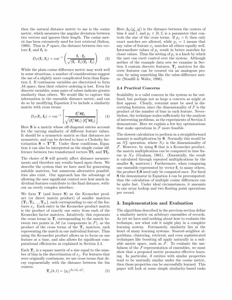
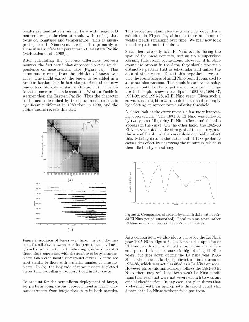
After calculating the pairwise differences betweenmonths, the first trend that appears is a striking de-pendence on measurement date (Figure 1a). Thisturns out to result from the addition of buoys overtime. One might expect the buoys to be added in arandom fashion, but in fact the positions of the newbuoys tend steadily westward (Figure 1b). This af-fects the measurements because the Western Pacific iswarmer than the Eastern Pacific. Thus the characterof the ocean described by the buoy measurements issignificantly different in 1980 than in 1990, and thecosine metric reveals this fact.

Year

Buo

y m

easu

rem

ents

per

mon

th

81 82 8384 85 86 87 88 89 90 91 92 93 94 95 96 97 98

1500

1000

500

0

(a)

80 82 84 86 88 90 92 94 96 98120 E

140 E

160 E

180 W

160 W

140 W

120 W

100 W

80 W

Year

Long

itude

(b)

Figure 1. Addition of buoys over time. In (a), the ma-trix of similarity between months (represented by back-ground shading, with dark indicating greater similarity)shows close correlation with the number of buoy measure-ments taken each month (foreground curve). Months aremost similar to those with a similar number of measure-ments. In (b), the longitude of measurements is plottedversus time, revealing a westward trend in later dates.

To account for the nonuniform deployment of buoys,we perform comparisons between months using onlymeasurements from buoys that exist in both months.

This procedure eliminates the gross time dependenceexhibited in Figure 1a, although there are hints ofweaker trends remaining over time. We may now lookfor other patterns in the data.

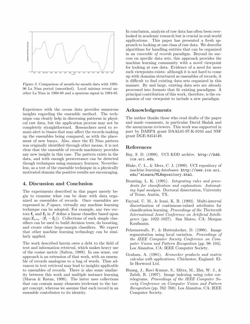
Since there are only four El Nino events during thespan of the measurements, setting up a supervisedlearning task seems overzealous. However, if El Ninoevents are present in the data, they should present adistinctive pattern that is self-similar and unlike thedata of other years. To test this hypothesis, we canplot the cosine scores of an El Nino period compared toall other observations. The result is somewhat noisy,so we smooth locally to get the curve shown in Fig-ure 2. This plot shows clear dips in 1982-83, 1986-87,1991-92, and 1997-98, all El Nino years. Given such acurve, it is straightforward to define a classifier simplyby selecting an appropriate similarity threshold.

A closer look at the curve reveals a few more interest-ing observations. The 1991-92 El Nino was followedby two years of lingering El Nino effect, and this alsoappears in the curve. On the other hand, the 1982-83El Nino was noted as the strongest of the century, andthe size of the dip in the curve does not really reflectthis. Missing data in the latter half of 1983 probablycauses this effect by narrowing the minimum, which isthen filled in by smoothing.

81 82 83 84 85 86 87 88 89 90 91 92 93 94 95 96 97 980.75

1.2

Year

Comp

ariso

n with

’82−

83 E

l Nino

even

t

Figure 2. Comparison of month-by-month data with 1982-83 El Nino period (smoothed). Local minima reveal otherEl Nino events in 1986-87, 1991-92, and 1997-98.

As a comparison, we also plot a curve for the La Ninayear 1995-96 in Figure 3. La Nina is the opposite ofEl Nino, so this curve should show minima in differ-ent spots. Indeed, the curve is high during El Ninoyears, but dips down during the La Nina year 1988-89. It also shows a fairly significant minimum around1984-85, which was not classified as a La Nina episode.However, since this immediately follows the 1982-83 ElNino, there may well have been weak La Nina condi-tions that year that were not severe enough to warrantofficial classification. In any case, the plot shows thata classifier with an appropriate threshold could stilldetect both La Ninas without false positives.

81 82 83 84 85 86 87 88 89 90 91 92 93 94 95 96 97 980.4

1.1

Year

Comp

ariso

n with

’95−

96 La

Nina

even

t

Figure 3. Comparison of month-by-month data with 1995-96 La Nina period (smoothed). Local minima reveal an-other La Nina in 1988-89 and a spurious signal in 1984-85.

Experience with the ocean data provides numerousinsights regarding the ensemble method. The tech-nique can clearly help in discerning patterns in physi-cal raw data, but the application process may not becompletely straightforward. Researchers need to re-main alert to biases that may affect the records makingup the ensembles being compared, as with the place-ment of new buoys. Also, since the El Nino patternwas originally identified through other means, it is notclear that the ensemble of records machinery providesany new insight in this case. The pattern exists in thedata, and with enough perseverance can be detectedthough techniques using summary features. Neverthe-less, as a test of the ensemble technique in a physicallymotivated domain the positive results are encouraging.

4. Discussion and Conclusion

The experiments described in this paper merely be-gin to examine what can be done with data orga-nized as ensembles of records. Once ensembles areexpressed in F -space, virtually any machine learningtechnique can be adopted. For example, any two vec-tors f1 and f2 in F define a linear classifier based uponsign (fnew · (f1 − f2)). Collections of such simple clas-sifiers can be used to build decision trees, do boosting,and create other large-margin classifiers. We expectthat other machine learning technology can be simi-larly applied.

The work described herein owes a debt to the field oftext and information retrieval, which makes heavy useof the cosine metric (Salton, 1989). In one sense, ourapproach is an extension of that work, with an ensem-ble of records analogous to a bag of words. Thus ad-vances in text retrieval may lead to insights applicableto ensembles of records. There is also some similar-ity between this work and multiple instance learning(Maron & Ratan, 1998). The latter uses collectionsthat can contain many elements irrelevant to the tar-get concept, whereas we assume that each record in anensemble contributes to its identity.

In conclusion, analysis of raw data has often been over-looked in academic research but is crucial in real-worldapplications. This paper has presented a fresh ap-proach to looking at one class of raw data. We describealgorithms for handling entities that can be organizedin an ensemble of records paradigm. Beyond its suc-cess on specific data sets, this approach provides themachine learning community with a novel viewpointfor looking at raw data. Evidence of a need for moresuch viewpoints exists: although it is not hard to comeup with domains structured as ensembles of records, itis difficult to find existing data sets organized in thismanner. By and large, existing data sets are alreadyprocessed into formats that fit existing paradigms. Aprincipal contribution of this work, therefore, is the ex-pansion of our viewpoint to include a new paradigm.

Acknowledgements

The author thanks those who read drafts of the paperand made comments, in particular David Skalak andthe anonymous reviewers. This work was supported inpart by DARPA grant DAAL01-97-K-0104 and NSFgrant DGE-9454149.

References

Bay, S. D. (1999). UCI KDD archive. http://kdd.ics.uci.edu.

Blake, C. L., & Merz, C. J. (1999). UCI repository ofmachine learning databases. http://www.ics.uci.edu/~mlearn/MLRepository.html.

Branting, L. K. (1991). Integrating rules and prece-dents for classification and explanation: Automat-ing legal analysis. Doctoral dissertation, Universityof Texas, Austin, TX.

Fayyad, U. M., & Irani, K. B. (1993). Multi-intervaldiscretization of continuous-valued attributes forclassification learning. Proceedings of the ThirteenthInternational Joint Conference on Artificial Intelli-gence (pp. 1022–1027). San Mateo, CA: MorganKaufmann.

Felzenszwalb, P., & Huttenlocher, D. (1998). Imagesegmentation using local variation. Proceedings ofthe IEEE Computer Society Conference on Com-puter Vision and Pattern Recognition (pp. 98–104).Los Alamitos, CA: IEEE Computer Society.

Graham, A. (1981). Kronecker products and matrixcalculus with applications. Chichester, England: El-lis Horwood Ltd.

Huang, J., Ravi Kumar, S., Mitra, M., Zhu, W. J., &Zabih, R. (1997). Image indexing using color cor-relograms. Proceedings of the IEEE Computer So-ciety Conference on Computer Vision and PatternRecognition (pp. 762–768). Los Alamitos, CA: IEEEComputer Society.

Kaelbling, L. P., Littman, M. L., & Moore, A. W.(1996). Reinforcement learning: A survey. Journalof Artificial Intelligence Research, 4, 257–285.

Kolodner, J. (1993). Case-based reasoning. San Mateo,CA: Morgan Kaufmann.

Maron, O., & Ratan, A. L. (1998). Multiple-instancelearning for natural scene classification. Proceed-ings of the Fifteenth International Conference onMachine Learning (pp. 341–349). San Mateo, CA:Morgan Kaufmann.

McPhaden, M. J., Kessler, W. S., & Soreide, N. N.(1999). El Nino story. http://www.pmel.noaa.gov/toga-tao/el-nino-story.html.

Salton, G. (1989). Automatic text processing – thetransformation, analysis, and retrieval of informa-tion by computer. Reading, MA: Addison Wesley.

Stanfill, C., & Waltz, D. (1986). Toward memory-based reasoning. Communications of the ACM, 29,1213–1228.

Swain, M., & Ballard, D. (1991). Color indexing. In-ternational Journal of Computer Vision, 7, 11–32.