Data Assimilation in 2D Magneto-Hydrodynamics Systems · Katholieke Universiteit Leuven Departement Elektrotechniek ESAT-SISTA/TR 04-74 Data Assimilation in 2D Magneto-Hydrodynamics

Katholieke Universiteit Leuven

Departement Elektrotechniek ESAT-SISTA/TR 04-74

Data Assimilation in

2D Magneto-Hydrodynamics Systems1

Oscar Barrero Mendoza, Dennis S. Bernstein2, and Bart L.R. De Moor3.

September 17, 2004

1This report is available by anonymous ftp from ftp.esat.kuleuven.ac.be in thedirectory pub/sista/barrero/reports/report04-156.ps.gz

2Dr. Dennis S. Berstein is a full professor at the Department of AerospaceEngineering, The University of Michigan, Ann Arbor, MI 48109-2140, USA

3Dr. Bart De Moor is a full professor at the Katholieke Universiteit Leuven, Bel-gium. Research supported by Research Council KUL: GOA-Mefisto 666, GOA-Ambiorics, several PhD/postdoc & fellow grants; Flemish Government: - FWO:PhD/postdoc grants, projects, G.0240.99 (multilinear algebra), G.0407.02 (sup-port vector machines), G.0197.02 (power islands), G.0141.03 (Identificationand cryptography), G.0491.03 (control for intensive care glycemia), G.0120.03(QIT), G.0452.04 (QC), G.0499.04 (robust SVM), research communities (IC-CoS, ANMMM, MLDM); - AWI: Bil. Int. Collaboration Hungary/ Poland; -IWT: PhD Grants, GBOU (McKnow) Belgian Federal Government: BelgianFederal Science Policy Office: IUAP V-22 (Dynamical Systems and Control:Computation, Identification and Modelling, 2002-2006), PODO-II (CP/01/40:TMS and Sustainibility); EU: FP5-Quprodis; ERNSI; Eureka 2063-IMPACT;Eureka 2419-FliTE; Contract Research/agreements: ISMC/IPCOS, Data4s,TML, Elia, LMS, IPCOS, Mastercard;

Abstract

Prediction of solar storms has become a very important issue due to the fact thatthey can affect dramatically the telecommunication and electrical power systems in theearth. As a result, a lot of research is being doing in this direction, space weather forecast.Magneto-Hydrodynamics systems are being studied in order to analyze the space plasmadynamics, and techniques which have been broadly used in prediction of earth environmen-tal variables like the Kalman filter (KF), the ensemble Kalman filter (EnKF), the extendedKalman filter (EKF), etc., are being studied and adapted to this new framework. Theassimilation of a wide range of space environment data into first-principles based globalnumerical models will improve our understanding of the physics of the geospace environ-ment and the forecasting of its behaviour. Therefore, the aim of this paper is to studythe performance of nonlinear observers in Magneto-Hidrodynamics systems, namely, theEnKF.

The EnKF is based on a Monte Carlo simulation approach for propagation of pro-cess and measurement errors. In this paper, the EnKF for a nonlinear two-dimensionalmagneto-hydrodynamic (2D-MHD) system is considered. For its implementation, twosoftware packages are merged, namely, the Versatile Advection Code (VAC) written inFortran and Matlab of Mathworks. The 2D-MHD is simulated with the VAC code whilethe EnKF is computed in Matlab. In order to study the performance of the EnKF inMHD systems, different number of measurement points as well as ensemble members areset.

1 INTRODUCTION 1

1 Introduction

In this paper, a first attempt is done for investigating the performance of the EnKF [4]in space weather forecast. Space weather forecast is an area of research that has becomevery active in the last years due to the need to predict solar storms. This solar storms canaffect dramatically the telecommunication and electrical power systems in the earth. Topredict such events data assimilation techniques can be used, data assimilation consists ofcombining physical first principle based models with measurements of the physical vari-ables in order to correct the estimation of these ones made by the model, due to the lackof information about initial conditions, boundary conditions, wrong and non-modelled dy-namics, etc. Hence, in order to make data assimilation for space weather, MHD equationsare used as basis for the physical first principle based model while EnKF for correctingthe estimation of the physical variables.

One of the motivation for using the EnKF is that it is very easy to implement dueto the fact that it is not needed any model linearization like the extended Kalman filter(EKF). Therefore, the EnKF can be set mainly into two modules; the model simulatorand the data assimilation module. These facts make the EnKF very attractive for realapplications. Hence, in this paper we use the VAC code [8] as the MHD simulator moduleand Matlab for the data assimilation module. Finally, the two codes are run simultane-ously using a script written in Matlab.

This paper is organized as follows, in the 2nd, 3rd and 4th sections the MHD systemand EnKF are introduced respectively. In the 5th section numerical results are presentedand finally in the 6th section some conclusions are given.

2 MHD system equations

The topic of MHD is ubiquitous in plasma physics. Examples where the theory has beenused with success range from explaining the spontaneous generation and subsequent evo-lution of magnetic fields within stellar and planetary interiors, to accounting for the grossstability of magnetically confined thermonuclear plasmas. Often, it is found that the scalelength of many instabilities and waves which are able to grow or propagate in a system arecomparable with the plasma size. It transpires that MHD is capable of providing a gooddescription of such large scale disturbances, indicating that the MHD account of plasmabehaviour is necessarily a macroscopic one. In essence, the theory is a marriage betweenfluid mechanics and electromagnetism. When compared with the extremely detailed par-ticle and kinetic theories, MHD is a relatively simple theory, perhaps even crude. Despiteits apparent simplicity, MHD describes a remarkably rich and varied mix of phenomenaand the subject is one whose development continues to flourish [2].

The basic equations of MHD can be summarized as follows:

2 MHD SYSTEM EQUATIONS 2

mass continuity:∂ρ

∂t+ ∇ · (ρ, υ) = 0, (1)

adiabatic equation of state:d

dt

(

p

ργ

)

= 0, (2)

momentum equation,

ρdυ

dt= J × B −∇p, (3)

Ampere’s law:∇× B = µ0J, (4)

Faraday’s law:

∇× E = −∂B

∂t, (5)

Gauss’ law:∇ · B = 0, (6)

resistive Ohm’s law:E + υ × B = ηJ, (7)

where each of the symbols has its customary meaning (see the list of symbols below), withthe convective derivative

d

dt,

∂

∂t+ υ · ∇

On the other hand, the right-hand side of (7) may be neglected to yield the ideal Ohm’slaw:

E + υ × B = 0 (8)

This states that there is no electric field in the rest frame of the fluid. Equations (1)-(6)with (8) constitute the ideal MHD equations, which is usually contracted to MHD. Theinclusion of (7) is described as resistive MHD.

An enormous amount of physics has been discarded in obtaining the MHD equations, soit is pertinent to enquire what precisely has been retained. It can be seen that the equationsare essentially an amalgam of fluids mechanics and ’pre-Maxwell’ electromagnetism. Thefluid inertia is affected by forces due to the fluid pressure gradients and to the J ×B term,which is the Lorentz force in continuum form. It will be noted however that the Ohm’slaw couples the fluid to the fields. If the magnetic flux is conserved, then this equationprovides constraints on the allowable class of fluid displacements described by the theory,and this in turn has implications for the topology of the magnetic fields.

MHD possesses those conservation properties enjoyed by fluid mechanics and electro-magnetism, namely:

• conservation of mass,

• conservation of momentum,

3 THE KALMAN FILTER 3

• conservation of energy (both mechanical and electromagnetic),

• conservation of magnetic flux.

list of symbols

µ0 - permeability of free space (N A2)η - resistivity of plasmaρ - average mass density of plasma (kg/m3)p - pressure (N/m2)γ - ratio of specific heatsv - velocity of the fluid element (m/s)J - current density (A/m2)E - electric fieldB - magnetic field

3 The Kalman Filter

Given a linear dynamical model on discrete form as

xk+1 = Akxk + Bkuk + wk, k ≥ 0, (9)

with output

yk = Ckxk + vk, (10)

where xk ∈ Rn, uk ∈ R

m, yk ∈ Rp, and Ak, Bk, Ck are known real matrices of appropriate

size. The input uk and output yk are assumed to be measured, and wk ∈ Rnk and vk ∈ R

p

are uncorrelated white noise processes with known variances and correlation given byQk, andRk, respectively.

3.1 Estimation Problem

Consider the discrete-time dynamical system described by (9) and (10). For this system,we take a state estimator of the form

xk|k = xk|k−1 + Lk(yk − yk|k−1), k ≥ 0, (11)

where Lk ∈ Rn×m and xk|k−1 is the estimate of xk based on observations up to time k−1,

with outputyk|k−1 = Cxk|k−1. (12)

In order to solve this problem a recursive procedure is used. The first step, is to projectahead xk−1|k−1 using (9)

xk|k−1 = Ak−1xk−1|k−1 + Bk−1uk−1, (13)

3 THE KALMAN FILTER 4

then, define the prior state estimation error by

ek|k−14= xk − xk|k−1, k > 0. (14)

Substituting (13) and (9) into (14) we obtain

ek|k−1 = Ak−1ek−1|k−1 + wk−1, (15)

now, define the prior error covariance matrix by

Pk|k−14= E[ek|k−1e

Tk|k−1], (16)

hence,

Pk|k−1 = Ak−1Pk−1|k−1ATk−1 + Qk−1. (17)

Next, define the state estimator error

ek|k4= xk − xk|k, (18)

consequently, the Kalman gain Lk minimizes

Jk(Lk) = tr(Pk|k), (19)

where the estimation error covariance matrix Pk|k ∈ Rn×n

Pk|k4= E[(ek|k − E[ek|k]])(ek|k − E[ek|k])

T ]. (20)

As a result, the Kalman gain can be obtained by

Lk = Pk|k−1CTk (Rk + CkPk|k−1C

Tk )−1, (21)

with the error covariance matrix update

Pk|k = (In − LkCk)Pk|k−1. (22)

Summarizing the algorithm we have for k = 1, 2, . . .

1. Project ahead the error covariance matrix and the estimated states:

Pk|k−1 = Ak−1Pk−1|k−1ATk−1 + Qk−1

xk|k−1 = Ak−1xk−1|k−1 + Bk−1uk−1

2. Compute the Kalman gain:

Lk = Pk|k−1CTk (Rk + CkPk|k−1C

Tk )−1

3. Update the estimated states:

xk|k = xk|k−1 + Lk(yk − yk|k−1)

4. Update the error covariance matrix:

Pk|k = (In − LkCk)Pk|k−1

4 THE ENSEMBLE KALMAN FILTER 5

4 The Ensemble Kalman Filter

The ensemble Kalman filter is a sequential data assimilation method where the errorstatistics are predicted by solving the Fokker-Planck equation (35), which describes thetime evolution of a probability density function of a model state, using a Monte Carloor ensemble integration. The method was originally proposed by [3]. By integrating anensemble of model states forward in time it is possible to calculate statistical moments likemean and error covariances whenever such information is required. Thus, all the statisticalinformation about the predicted model state that is required at analysis times is containedin the ensemble.

The method is presented in three stages:

• Representation of error statistics

• Prediction of error statistics

• The estimation problem

4.1 Representation of Error Statistics

The error covariance matrices for the prior and the current estimate, Pk|k−1 and Pk|k, arein the Kalman filter defined in terms of the true state as

Pk|k−1 = E[

(xk − xk|k−1)(xk − xk|k−1)T]

(23)

Pk|k = E[

(xk − xk|k)(xk − xk|k)T]

(24)

where E[·] denotes an expectation value. Now, for the EnKF assume that we have anensemble of forecasted model states that randomly sample the model errors at time k.Let’s denote this ensemble as Xk|k−1 and is defined by

Xk|k−14= (x1

k|k−1, . . . , xNk|k−1), (25)

where the superscript denotes the ensemble member. Then, the ensemble mean ¯xk|k−1 isdefined by

¯xk|k−14=

1

N

N∑

i=1

xj

k|k−1. (26)

Since the true state xk is not known, and in order to write (23) and (24) in terms of(25), we therefore define the ensemble covariance matrices around the ensemble mean asfollows; define the ensemble of prior estimation errors by

Ek|k−14= (x1

k|k−1 − ¯xk|k−1, . . . , xNk|k−1 − ¯xk|k−1), (27)


and the ensemble of estimation errors by

Ek|k4= (x1

k|k − ¯xk|k, . . . , xNk|k − ¯xk|k). (28)

Hence,

Pk|k−1 ≈ Pk|k−14=

1

N − 1E

[

Ek|k−1ETk|k−1

]

, (29)

Pk|k ≈ Pk|k4=

1

N − 1E

[

Ek|kETk|k

]

, (30)

which are averages over the ensembles. Thus, we can use an interpretation where theensemble mean is the best estimate and the spreading of the ensemble around the mean isa natural definition of the error in the ensemble mean. Since the error covariances definedin (29) and (30) are defined as ensemble averages, there will clearly exist infinitively manyensembles with an error covariance equal to Pk|k−1 and Pk|k. Thus, instead of storinga full covariance matrix, we can represent the same error statistics using an appropriateensemble of model states. Given an error covariance matrix, an ensemble of finite sizewill always provide an approximation to the error covariance matrix. However, when thesize of the ensemble N increases the errors in the Monte Carlo sampling will decreaseproportional to 1/

√N .

Suppose now that we have N model states in the ensemble, each of dimension n. Eachof these model states can be represented as a single point in an N -dimensional state space.All the ensemble members together will constitute a cloud of points in the state space.Such a cloud of points in the state space can, in the limit when N goes to infinity, bedescribed using a probability density function

φ(x) =dN

N, (31)

where dN is the number of points in a small unit volume and N is the total numberof points. With knowledge about either or the ensemble representing we can calculatewhichever statistical moments (such as mean, covariances etc.) we want whenever theyare needed.

The conclusion so far is that the information contained by a full probability densityfunction can be exactly represented by an infinite ensemble of model states.

4.2 Prediction of Error Statistics

The EnKF was designed to resolve two major problems related to the use of the extendedKalman filter (EKF) with nonlinear dynamics in large state spaces. The first problemrelates to the use of an approximate closure scheme in the EKF, and the other to thehuge computational requirements associated with the storage and forward integration ofthe error covariance matrix. The EKF applies a closure scheme where third- and higherorder moments in the error covariance equation are discarded. This linearization has beenshown to be invalid in a number of applications. In fact, the equation is no longer the


fundamental equation for the error evolution when the dynamical model is nonlinear. Fora nonlinear model where we appreciate that the model is not perfect and contains modelerrors, we can write it as a discrete-time stochastic differential equation as

xk+1 = A(xk) + ηk (32)

with ηk the model error at time k defined by

ηk4= Gk(xk)δk, (33)

with Gk(xk) ∈ Rn×l is a state-dependent matrix, where the covariance matrix Qk ∈ R

n×n

is defined as

Qk4= E[Gk(xk)Gk(xk)

T], (34)

and δk ∈ Rl is a process we want to approximate as white noise. Equation (32) implies

that even if the initial state is known precisely, future model sates cannot since unknownrandom model errors are continually added.

Conceptually, the evolution of (31) can be modelled with the Fokker-Planck equation

∂φ(xk)

∂t= −∇ ·

[

A(xk)φ(xk)]

+∑

i,j

∂2

∂xk(i)∂xk(j)

(Qk

2

)

ijφ(xk) (35)

This equation does not apply any important approximations and can be considered asthe fundamental equation for the time evolution of error statistics. A detailed derivationis given in [5]. The equation describes the change of the probability density in a localvolume which is dependent on the divergence term describing a probability flux into thelocal volume (impact of the dynamical equation) and the diffusion term which tends toflatten the probability density due to the effect of stochastic model errors. If (35) couldbe solved for the probability density function, it would be possible to calculate statisticalmoments like the mean state and the error covariance for the model forecast to be used inthe analysis scheme. The EnKF applies a so called Markov Chain Monte Carlo (MCMC)method to solve (35). The probability density can be represented using a large ensembleof model states. By integrating these model states forward in time according to the modeldynamics described by (32), this ensemble prediction is equivalent to solving the Fokker-Planck equation using a MCMC method. This procedure forms the backbone for theEnKF.

4.3 The Estimation Problem

In the standard KF estimation problem the definition of Pk|k−1 and Pk|k are used. It isnow given a derivation of the estimation problem for the EnKF using (29) and (30).

The EnKF performs an ensemble of parallel data assimilation cycles, using (11) asfollows,


for i = 1, . . . , N

xik|k = xi

k|k−1 + Lek

(

yik − C(xi

k|k−1))

, (36)

where C is the observation operator, which is permitted to be a nonlinear operator, andthe observations yi

k = yk + εi are perturbed observations defined such that εi ∼ N(0, Re).In the limit of an infinite ensemble the matrix Re will converge toward the prescribed errorcovariance matrix R used in the standard KF.

Similar to the standard KF, In (36) Lekis defined as

Lek= Pk|k−1C

T(CPk|k−1CT + Re)

−1, (37)

with the difference that C can be nonlinear which is a powerful advantage compare to othernon-linear KF that are based on linearized models like EKF. Envision a situation whereerrors grow rapidly but saturate at low amplitude; the linear assumption of error growthin the EKF will result in an overestimate of the prior error variance, but the differencesamong ensemble members will not grow without bound and thus should provide a moreaccurate model of the actual prior error statistics.

On the other hand, for a complex model with a high-dimensional state vector, ex-plicitly forming Pk|k−1 as in (29) would be computationally prohibitive. However, in the

EnKF, Lekcan be formed without ever explicitly computing the full Pk|k−1. Instead, the

components of Pk|k−1CT and CPk|k−1C

T of Lekare computed separately. Define

C(xk|k−1)4=

1

N

N∑

i=1

C(xik|k−1), (38)

which represents the mean of the estimate of the observation interpolated from the back-ground forecasts. Then

Pk|k−1CT 4

=1

N − 1

N∑

i=1

(

xik|k−1 − ¯xk|k−1

)(

C(xik|k−1) − C(xk|k−1)

)T, (39)

and

CPk|k−1CT 4

=1

N − 1

N∑

i=1

(


)(


)T, (40)

After the estimation is done, a short-range forecast is computed by running the physicsfirst principle based model (32) until new measurements are taken, then the data assimi-lation is repeat it.

5 NUMERICAL RESULTS 9

5 Numerical Results

In order to investigate how the EnKF operates in MHD systems, we took the ideal MHDsystem equations (1)-(6) with (8), setting the boundary conditions of the right-hand sidesuch that it simulates the magnetosphere around the earth. This system was simulatedwith the VAC code with the following parameters:

• Grid size: 34 × 54

• Initial conditions of the state space variables:

– Mass density, ρ = 1.0Kg/m3

– Velocity in x- and y-directions, Vx = 20m/s, Vy = 0m/s

– Pressure, p = 1.0Kg/ms2

– Magnetic field in x- and y-directions, Bx = 0mT , By = 1.0mT

• ratio of specific heats, γ = 5/3

• Simulation sample time, 1 × 10−4 seconds

• Data assimilation sample time, 4 × 10−4 seconds

• Spatial discretization method, Total Variation Diminishing Lax-Friedrich, TVDLF.

As a result the order of the system is 11016, 6 state space variables and 34×54 gridpoints.To excite the system, a square sinusoidal wave for By and Vx was generated at the left-hand boundary, simulating a magnetic storm. The variation of By were from 1 to 1.5 mTwhile for Vx from 20 to 30 m/s.

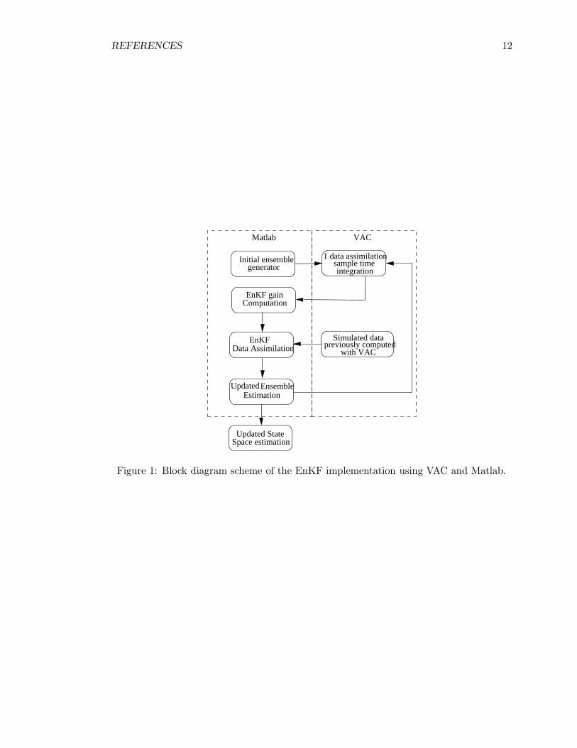
Figure 1 depicts a general scheme of the EnKF implementation by running Matlab andthe VAC code simultaneously. Since we can see in the scheme we did not need any extracode for the model, anyhow we had to write the code of the EnKF in Matlab, and somecode to read and write the VAC’s files where the initial and final conditions in each data-assimilation time-step are saved. As a result, we have got an modular data-assimilationsystem where the nonlinear model integration module is executed by the VAC code, whilethe data assimilation module for Matlab. This is one of the motivation for using the EnKF,because it is quite straightforward to implement, and the results are very confident.

To investigate the performance of the EnKF in MHD systems a magnetic storm aroundthe earth was simulated by changing the boundary conditions as mentioned above. Westudy three cases, for 10, 100, and 200 measurement points, and for each case we use 50,150, and 300 ensemble members, respectively.

Figure 2 shows the root mean square error (RMSE) of the state space estimationfor the whole scenarios. On the first column, when 50 ensemble members are used, canbe seen that the data assimilation process always crashes independent of the number ofmeasurement points, this is due to the fact that the number of ensemble members is smallcompare to the order or the system, hence, it is difficult for the EnKF to describe very

6 CONCLUSIONS 10

well the statistics of system, taking the system to regions where the model integrationbecomes unfeasible.

In the other cases, 150 and 300 members, the data assimilation process works morereliable, even for the cases with 10 measurement points. Although the worst performanceis for the case of 10 measurement points with 150 and 300 ensemble members, the resultsare closed to the other cases indicating that the number of ensemble members is moreimportant than the number of measurement points; however the number and the locationof the measurement points is important as well. In the experiments the location of themeasurement point are chosen such that at least half of the points were located in the right-half plane around the bowshock where the more drastic changes occurs, this guaranteesthat the data assimilation process will track the big changes in the system, otherwise theestimation would be very poor.

Figures 3-5, and 6-8 depict how the magnetic field and the plasma velocity around theearth are estimated respectively for the different cases. It can be seen clearer that themore ensemble members and measurement points are taken, the better the estimation is,as expected.

6 Conclusions

In this paper we introduced a new area of application for the EnKF, space weather forecast.The EnKF is an extension of the Kalman filter to the nonlinear case, where based on aMonte Carlo simulation approach the measurement and process noise errors are propa-gated. One of the advantages of the EnKF is its facility to be implemented as a modularsystem, with mainly two modules, namely, the model simulator and the data assimilationmodule. This scheme permits the use of specialized codes for each task, making the EnKFmore robust and reliable.

The EnKF performed very well in the experiment shown. The results are very promis-ing in the sense that with few measurement points located strategically, we can obtain agood estimation of the dynamics of the system. We mention this, because in the real casethere are very few satellites out there in the space which can be used as measurementpoints.

One of the drawbacks of the EnKF is that it is very demanding computationally,despite the fact that one can represent the statistics with a few number of ensemblemembers compared to the size of the system. Also the knowledge of the process andmeasurement noise are needed in order to have more accurate results.

7 Acknowledgment

Dr. Bart De Moor is a full professor at the Katholieke Universiteit Leuven, Belgium.Research supported by Research Council KUL: GOA-Mefisto 666, GOA-Ambiorics, sev-eral PhD/postdoc & fellow grants; Flemish Government: - FWO: PhD/postdoc grants,projects, G.0240.99 (multilinear algebra), G.0407.02 (support vector machines), G.0197.02

REFERENCES 11

(power islands), G.0141.03 (Identification and cryptography), G.0491.03 (control for in-tensive care glycemia), G.0120.03 (QIT), G.0452.04 (QC), G.0499.04 (robust SVM), re-search communities (ICCoS, ANMMM, MLDM); - AWI: Bil. Int. Collaboration Hungary/Poland; - IWT: PhD Grants, GBOU (McKnow) Belgian Federal Government: Belgian Fed-eral Science Policy Office: IUAP V-22 (Dynamical Systems and Control: Computation,Identification and Modelling, 2002-2006), PODO-II (CP/01/40: TMS and Sustainibil-ity); EU: FP5-Quprodis; ERNSI; Eureka 2063-IMPACT; Eureka 2419-FliTE; ContractResearch/agreements: ISMC/IPCOS, Data4s, TML, Elia, LMS, IPCOS, Mastercard.

References

[1] G.P. Burgers, P.J Van Leeuwen and G. Evensen, Analysis scheme in the ensembleKalman filter, Monthly Weather Review, 1998, vol. 126, pp. 1719-1724.

[2] R. Dendy, Plasma Physics: an Introductory Course, 1st edition, Cambridge UniversityPress, 1996.

[3] G. Evensen, Sequential data assimilaion with a nonlinear quasigeostrophic modelusing Monte Carlo methods to forecast error statistics, Geophys. Res., 1994, vol.99-C5, pp. 10143-10162.

[4] G. Evensen, The ensemble Kalman filter: theroretical formulation and practical im-plementation, Ocean Dynamics, 2003, vol. 53, pp. 343-367.

[5] A.H. Jazwinski, Stochastic processes and filtering theory, Academic Press, 1970.

[6] R.E. Kalman, A new approach to linear filtering and prediction problems, Transac-tions of hte AMSE-Journal of Basic Engineering, 1960, vol. 83D, pp. 35-45.

[7] R.E. Kalman and R.S. Bucy, New results in linear filtering and prediction theory,Transactions of hte AMSE-Journal of Basic Engineering, 1961, vol. 83D, pp. 95-108.

[8] G. Toth and R. Keppens, Versatile Advection Code, Universiteit Utrecht, The Nether-lands, 2003.

[9] A.C. Lorenc, Analysis methods for numerical weather prediction, Quart. J. Roy. Me-teor. Soc., 1986, vol. 112, pp. 1177-1194.

[10] D.F. Parrish and J.C. Derber, The National Meteorological Center’s Spectral Sta-tistical Interpolation Analysis System, Monthly Weather Review, 1992, vol. 120, pp.1747-1763.

REFERENCES 12

EnKF gainComputation

1 data assimilationsample time integration

Simulated datapreviously computed

with VAC

Space estimationUpdated State

generatorInitial ensemble

UpdatedEnsembleEstimation

Data AssimilationEnKF

VACMatlab

Figure 1: Block diagram scheme of the EnKF implementation using VAC and Matlab.

REFERENCES 13

050

100

0

1000

2000

e

50 m

emb.

050

100

0

100

200

150

ense

m. m

emb.

050

100

050100

150

300

ense

m. m

emb.

050

100

0

1000

2000

V

050

100

0510

050

100

0246

050

100

0510

B

itera

tions

050

100

0123

itera

tions

050

100

0123

itera

tions

Figure 2: Comparison of the performance of the EnKF for different number of mea-surement points as well as ensemble members, where e-energy density, V-velocity, andB-Magnetic field. Dotted line; RMSE for 10 measurement points, dashed line; RMSE for100 measurement points, and solid line; RMSE for 200 measurement points.

REFERENCES 14

k=

1

Best

150 ens.

0.2

0.4

0.6

0.8

1

2

3

Best

300 meas.

1

2

3

Breal

2

3

4k=

40

0.2

0.4

0.6

0.8

2

4

6

2

4

6

2

4

6

k=

70

0.2

0.4

0.6

0.8

24681012

24681012

5

10

15

k=

110

0.05 0.1 0.15

0.2

0.4

0.6

0.8

5

10

15

0.05 0.1 0.15

24681012

0.05 0.1 0.15

5

10

15

Figure 3: Comparison of performance for the case of 10 measurement points. At thetop-right, the big dots are the location of the measurement points on the grid.

REFERENCES 15

k=

1

Best

150 ens.

0.2

0.4

0.6

0.8

Best

300 meas. Breal

k=

40

0.2

0.4

0.6

0.8

k=

70

0.2

0.4

0.6

0.8

k=

110

0.05 0.1 0.15

0.2

0.4

0.6

0.8

0.05 0.1 0.15 0.05 0.1 0.15

1

2

3

1

2

3

2

3

4

1

2

3

4

5

2

4

6

2

4

6

24681012

5

10

15

5

10

15

2

4

6

8

10

2

4

6

8

10

5

10

15


REFERENCES 16

k=

1

Best

150 ens.

0.2

0.4

0.6

0.8

Best

300 meas. Breal

k=

40

0.2

0.4

0.6

0.8

k=

70

0.2

0.4

0.6

0.8

k=

110

0.05 0.1 0.15

0.2

0.4

0.6

0.8

0.05 0.1 0.15 0.05 0.1 0.15

1

2

3

1

2

3

2

3

4

2

4

6

1

2

3

4

5

2

4

6

5

10

15

5

10

15

5

10

15

5

10

15

24681012

5

10

15


REFERENCES 17

k=

1

Vest

150 ens.

0.2

0.4

0.6

0.8

5

10

15

Vest

300 ens.

5

10

15

20

Vreal

5

10

15k=

40

0.2

0.4

0.6

0.8

5

10

15

20

25

10

20

30

5

10

15

20

k=

70

0.2

0.4

0.6

0.8

10

20

30

40

50

10

20

30

40

50

5

10

15

20

k=

110

0.05 0.1 0.15

0.2

0.4

0.6

0.8

10

20

30

0.05 0.1 0.15

10

20

30

0.05 0.1 0.15

5

10

15


REFERENCES 18

k=

1

Vest

150 ens.

0.2

0.4

0.6

0.8

Vest

300 ens. Vreal

k=

40

0.2

0.4

0.6

0.8

k=

70

0.2

0.4

0.6

0.8

k=

110

0.05 0.1 0.15

0.2

0.4

0.6

0.8

0.05 0.1 0.15 0.05 0.1 0.15

5

10

15

20

5

10

15

20

5

10

15

10

20

30

10

20

30

5

10

15

20

10

20

30

5

10

15

20

25

5

10

15

20

10

20

30

40

50

5

10

15

20

25

5

10

15


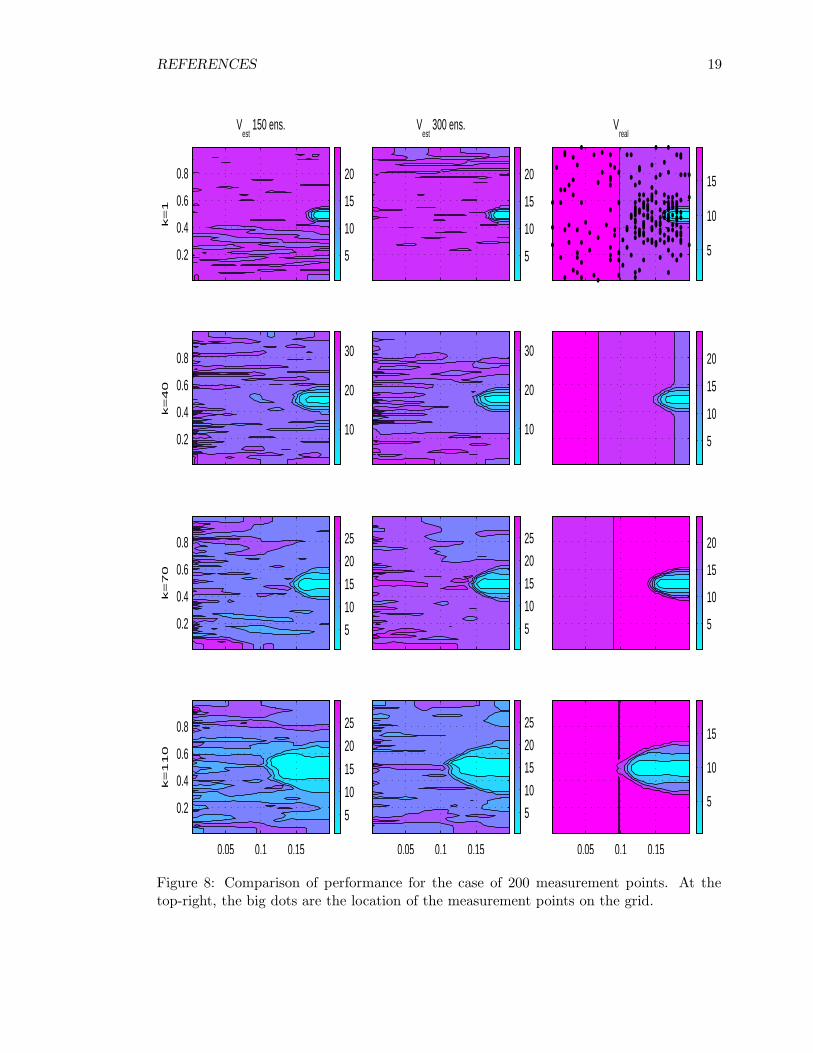
REFERENCES 19

k=

1

Vest

150 ens.

0.2

0.4

0.6

0.8

Vest

300 ens. Vreal

k=

40

0.2

0.4

0.6

0.8

k=

70

0.2

0.4

0.6

0.8

k=

110

0.05 0.1 0.15

0.2

0.4

0.6

0.8

0.05 0.1 0.15 0.05 0.1 0.15

5

10

15

20

5

10

15

20

5

10

15

10

20

30

10

20

30

5

10

15

20

5

10

15

20

25

5

10

15

20

25

5

10

15

20

5

10

15

20

25

5

10

15

20

25

5

10

15


Documents

Data Assimilation in 2D Magneto-Hydrodynamics Systems · Katholieke Universiteit Leuven Departement Elektrotechniek ESAT-SISTA/TR 04-74 Data Assimilation in 2D Magneto-Hydrodynamics