Data-capture and analysis with the BBC micro:bit and Microsoft MakeCode block editor and App.

Adrian Oldknow March 2018 adrian@ccite.org

The micro:bit has built-in sensors e.g. for acceleration, magnetic field, temperature and light

intensity. It also has a large number (>20) of input/output pins capable of reading and writing both

digital and analog data. It can exchange data with other devices either through the USB cable, or

with Bluetooth Low-Energy radio, or with full Bluetooth connection. The current Microsoft’s

MakeCode JavaScript blocks editor runs in a browser and provides a very easy to use, Scratch like,

graphical programming system for the micro:bit. Together, micro:bits and MakeCode provide a

very easy to use and low-cost gateway into physical computing, accessible to students learning

STEM subjects at KS2/3 (8-14 years). Circuits can be built with very common and cheap electronic

components familiar in secondary school science and DT departments for teaching electronics to

older students. There are also several UK companies which have developed relatively cheap kits to

help learners explore microelectronics and robotics with micro:bits, such as Kitronik, 4Tronik and

MonkMakes. There is also a range of resources to help learn the key principles, such as at STEM

Learning, Dendrite and at TechAgeKids.

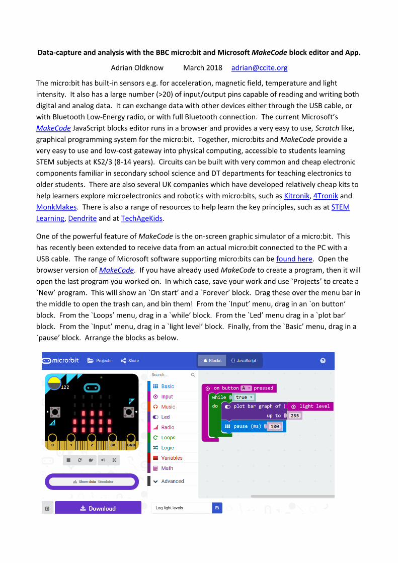
One of the powerful feature of MakeCode is the on-screen graphic simulator of a micro:bit. This

has recently been extended to receive data from an actual micro:bit connected to the PC with a

USB cable. The range of Microsoft software supporting micro:bits can be found here. Open the

browser version of MakeCode. If you have already used MakeCode to create a program, then it will

open the last program you worked on. In which case, save your work and use `Projects’ to create a

`New’ program. This will show an `On start’ and a `Forever’ block. Drag these over the menu bar in

the middle to open the trash can, and bin them! From the `Input’ menu, drag in an `on button’

block. From the `Loops’ menu, drag in a `while’ block. From the `Led’ menu drag in a `plot bar’

block. From the `Input’ menu, drag in a `light level’ block. Finally, from the `Basic’ menu, drag in a

`pause’ block. Arrange the blocks as below.

In order to test the program just press button A in the simulator. A simulated light sensor shows in

the upper left corner. With the mouse, you can drag the light level up and down. The greater the

light level, the greater the number of LEDs are displayed.

As it stands, the program has no means of

stopping. But there is a `pause’ button beneath

the simulator. Extend the program as shown.

Use the `Variables’ menu to bring in a `set’

block. Use the little red arrow next to the

`item’ and rename the variable to `state’. Use

the `Logic’ menu to drag in a `true’ block. From

the `Input’ menu, drag in another `on button’

block, and use the down arrow to change `A’ to

`B’. Now we can press A to start data-logging

and use button B to stop it. The recently added

feature is the `Show data’ button beneath the

simulator. Click on the `on start’ block to

restart the program. You may need to press the

`refresh’ button under the simulator. Press button

A to restart data collection, then drag the light-level

simulator up and down to check that the LEDs work according to plan. Then press the `Show data’

bar to show how the streamed data graph changes as you move the light level in the simulator.

Press the green `pause’ button above the simulator. The blue symbol next to it is used to create a

file from the data. This is saved to your PC as a text file in a standard format called `comma

separated variable’, CSV, format. This can be opened in a spreadsheet, such as Microsoft Excel, for

manipulation and analysis. In order to capture live data on the PC from the micro:bit we need to

move to the new beta version of the MakeCode editor as a Windows 10 App.

With the program uploaded to a micro:bit, the actual program should send data back down the USB

cable so that an additional `Show data’ button appears, this time labelled `Device’ rather than

`Simulator’. Then you can press button A on the micro:bit, check that the LEDs change as you move

it nearer or further from a light source and then press `Show data Device’ to start graphing and

logging the data. Press the `Pause’ and Download’ buttons to save the actual data as a CSV file.

This has not, at the time of writing, been fully implemented in the browser version of MakeCode.

However there is now a free-standing Windows 10 App in development for MakeCode. You can

install it free from the Windows App Store. Whenever you include a `plot bar graph’ block in a

program, the micro:bit will send the data back down the USB cable as well as showing LEDs on its

display. Here is an example of the light level program running in action, rather than simulated.

When you download the data

using the blue button at the top

right, the data is written to your

PC as a CSV file and automatically

opens in Excel. The elapsed times

in seconds are store in the A

column, and the light levels from

`source 1’ are stored in column B.

Inserting a scattergraph of B against A recaptures the data graph shown on MakeCode.

You can also use `Advanced’ to reveal the `Serial’ menu and use `serial write number’ and `serial

write line’ blocks to control exactly what is sent back down the USB cable to MakeCode.

Now when you use `Show data’ you will see the stream of numbers being sent as well as their

graph.

Now we have explored the new MakeCode tools for data-capture and display we can set up a more

realistic scientific experiment. The one I have chosen is for the classic capacitor discharge model.

In science we often meet models of simple linear relations such as Ohms law: V = iR. Using a

variable resistor (potentiometer) we can easily find that, for a fixed voltage V, the current i and the

resistance R are `inversely proportional’ – the greater the resistance, the lower the voltage, and

vice versa. The graph of i against R is a straight line of negative gradient. The classical models of

growth and decay are similar but it is the rate of growth which is proportional to the quantity being

observed. The Malthus model for unconstrained growth is that the greater the population the

faster the population grows. Newton’s law of cooling is a `decay’ model. The closer the

temperature of an object is to its environment, the slower it cools. When a capacitor has been

charged up fully and is then disconnected, its voltage will decay towards zero, but no steadily. The

greater its voltage, the faster it decays. Growth and decay are important phenomenon, but made

more complex by the terms `exponential growth’, like populations, and `exponential decay’, like

temperature and discharge.

For my experiment I have adapted the circuit and code from

Experiment 9 `Capacitor Discharge Circuit’ from the Kitronik Inventor’s

kit. The photo shows the circuit. There are two switches and a

potentiometer. There is also a 220 μF capacitor and two 2.2kΩ

resistors. The positive side of the capacitor is connected to pin P0.

Holding down the right-hand switch charges the capacitor. The rate is

determined by the setting of the potentiometer. The micro:bit’s LEDs

show the voltage increasing to a maximum of 3V voltage. Holding

down the left-hand switch discharges the capacitor back down to 0V.

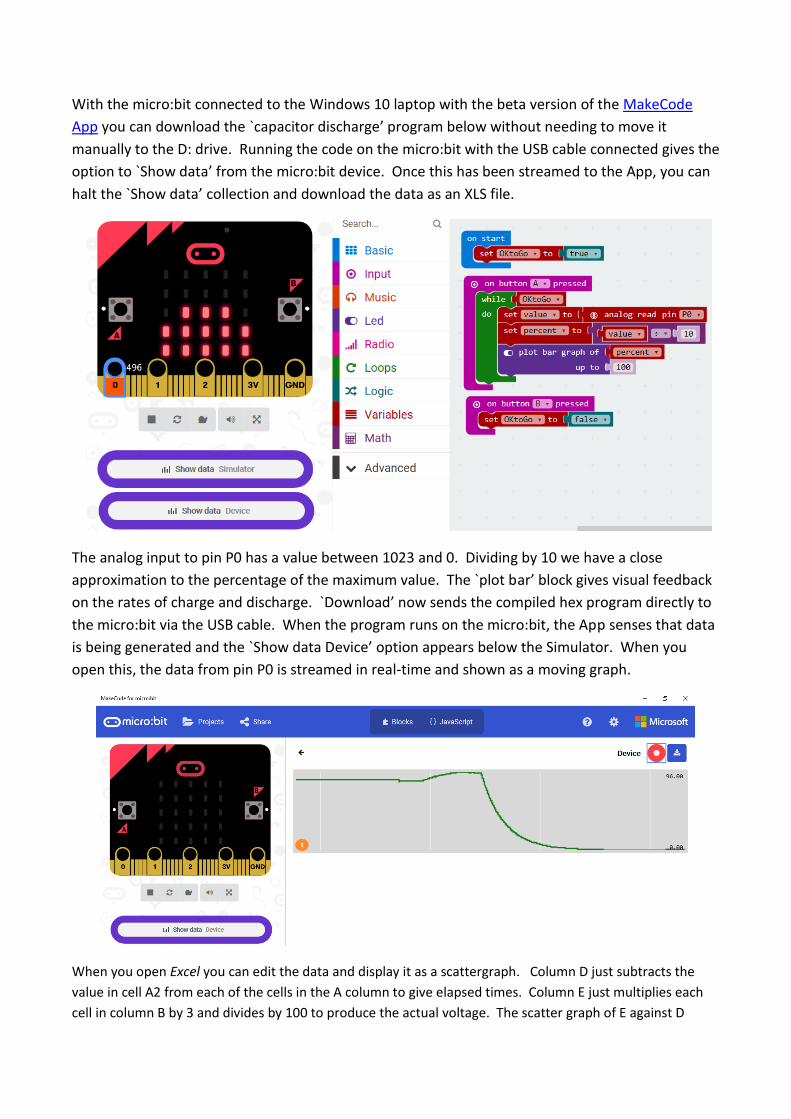
With the micro:bit connected to the Windows 10 laptop with the beta version of the MakeCode

App you can download the `capacitor discharge’ program below without needing to move it

manually to the D: drive. Running the code on the micro:bit with the USB cable connected gives the

option to `Show data’ from the micro:bit device. Once this has been streamed to the App, you can

halt the `Show data’ collection and download the data as an XLS file.

The analog input to pin P0 has a value between 1023 and 0. Dividing by 10 we have a close

approximation to the percentage of the maximum value. The `plot bar’ block gives visual feedback

on the rates of charge and discharge. `Download’ now sends the compiled hex program directly to

the micro:bit via the USB cable. When the program runs on the micro:bit, the App senses that data

is being generated and the `Show data Device’ option appears below the Simulator. When you

open this, the data from pin P0 is streamed in real-time and shown as a moving graph.

When you open Excel you can edit the data and display it as a scattergraph. Column D just subtracts the

value in cell A2 from each of the cells in the A column to give elapsed times. Column E just multiplies each

cell in column B by 3 and divides by 100 to produce the actual voltage. The scatter graph of E against D

shows how the voltage decays with time when the capacitor discharges The `trend line’ shows a nice

negative exponential decay!

We can also `prune’ the data in columns D and E by deleting rows where data has been duplicated.

Copying the resulting data in columns D and E allows us to paste the values into other applications

such as the free, open-source GeoGebra software.

The screen shot shows several of GeoGebra’s Views. The data from Excel has been pasted to the

Spreadsheet View on the right. That has a `Two variable regression analysis’ option, like the `trend-

line’ in Excel. Selecting columns A and B you can use this both to create the scattergram and to

compute the best fit for a number of possible regression models, including exponential. The red

graph is the best fit exponential function and its equation is shown in the Algebra View on the left.

The scattergram and graph appear in the Graphics View in the middle. Here we can create a

segment on the x-axis, shown in purple. The point C has been created to slide on this segment. The

perpendicular to the x-axis through C cuts the red graph at D. The tangent to the red graph at D is

drawn in brown. Its gradient is measured and stored as `slope’. The length of CD represents the

current voltage and its length is also measured and stored as `volts’. In the Input bar I have entered

the formula `ratio = slope/volts’ to define the ratio of slope to volts. This is written on Graphics

View as a text box. You can drag C along the segment AB to see that while the values of volts and

slope change, their ratio stays constant. You can also animate the point C using the start/stop

button in black at the bottom left corner of the Graphics View. So we have a very convincing

demonstration that the more the stored voltage the faster the capacitor discharges – which is what

we mean by a negative exponential decay. You can access the GeoGebra `Capacitor discharge’ file

from GeoGebra Tube.

Further examples of science experiments explored using micro:bits are on the MakeCode site, as

well as an extensive Computer Science course on micro:bits. Many thanks to all the folk at the

Micro:bit Educational Foundation and Microsoft who have made such a lovely tool available at just

the right time.