Data Compression, 4th Edition. Program and Pseudo … Compression, 4th Edition. Program and Pseudo-Code Listings (Advise the author about missing or bad listings.) Chapter 1 % Returns

Data Compression, 4th Edition. Program and Pseudo-Code Listings

(Advise the author about missing or bad listings.)

Chapter 1

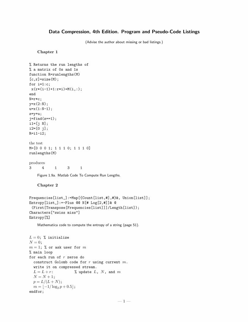
% Returns the run lengths of% a matrix of 0s and 1sfunction R=runlengths(M)[c,r]=size(M);for i=1:c;x(r*(i-1)+1:r*i)=M(i,:);endN=r*c;y=x(2:N);u=x(1:N-1);z=y+u;j=find(z==1);i1=[j N];i2=[0 j];R=i1-i2;

the testM=[0 0 0 1; 1 1 1 0; 1 1 1 0]runlengths(M)

produces3 4 1 3 1

Figure 1.9a. Matlab Code To Compute Run Lengths.

Chapter 2

Frequencies[list_]:=Map[{Count[list,#],#}&, Union[list]];Entropy[list_]:=-Plus @@ N[# Log[2,#]]& @(First[Transpose[Frequencies[list]]]/Length[list]);Characters["swiss miss"]Entropy[%]

Mathematica code to compute the entropy of a string (page 51).

L = 0; % initializeN = 0;m = 1; % or ask user for m% main loopfor each run of r zeros doconstruct Golomb code for r using current m.write it on compressed stream.L = L + r: % update L, N, and mN = N + 1;p = L/(L + N);m = �−1/ log2 p + 0.5�;

endfor;

— 1 —

Data Compression (4th Edition): Verbatim Listings

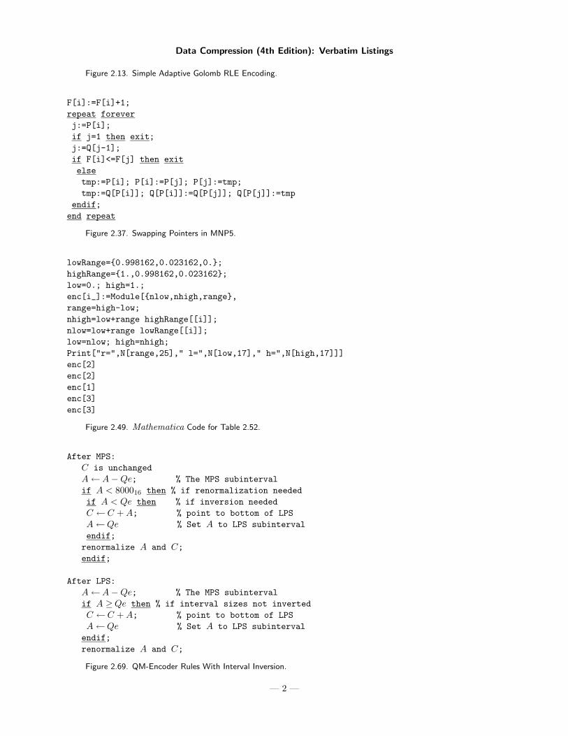
Figure 2.13. Simple Adaptive Golomb RLE Encoding.

F[i]:=F[i]+1;repeat foreverj:=P[i];if j=1 then exit;j:=Q[j-1];if F[i]<=F[j] then exitelsetmp:=P[i]; P[i]:=P[j]; P[j]:=tmp;tmp:=Q[P[i]]; Q[P[i]]:=Q[P[j]]; Q[P[j]]:=tmp

endif;end repeat

Figure 2.37. Swapping Pointers in MNP5.

lowRange={0.998162,0.023162,0.};highRange={1.,0.998162,0.023162};low=0.; high=1.;enc[i_]:=Module[{nlow,nhigh,range},range=high-low;nhigh=low+range highRange[[i]];nlow=low+range lowRange[[i]];low=nlow; high=nhigh;Print["r=",N[range,25]," l=",N[low,17]," h=",N[high,17]]]enc[2]enc[2]enc[1]enc[3]enc[3]

Figure 2.49. Mathematica Code for Table 2.52.

After MPS:C is unchangedA ←A − Qe; % The MPS subintervalif A < 800016 then % if renormalization neededif A < Qe then % if inversion neededC ←C + A; % point to bottom of LPSA ←Qe % Set A to LPS subintervalendif;

renormalize A and C;endif;

After LPS:A ←A − Qe; % The MPS subintervalif A ≥Qe then % if interval sizes not invertedC ←C + A; % point to bottom of LPSA ←Qe % Set A to LPS subinterval

endif;renormalize A and C;

Figure 2.69. QM-Encoder Rules With Interval Inversion.

— 2 —


Chapter 3

(QIC-122 BNF Description)<Compressed-Stream>::=[<Compressed-String>] <End-Marker><Compressed-String>::= 0<Raw-Byte> | 1<Compressed-Bytes><Raw-Byte> ::= (8-bit byte)<Compressed-Bytes> ::=<offset><length><offset> ::= 1 (a 7-bit offset)

|0 (an 11-bit offset)

<length> ::= (as per length table)<End-Marker> ::=110000000 (Compressed bytes with offset=0) ::=0|1

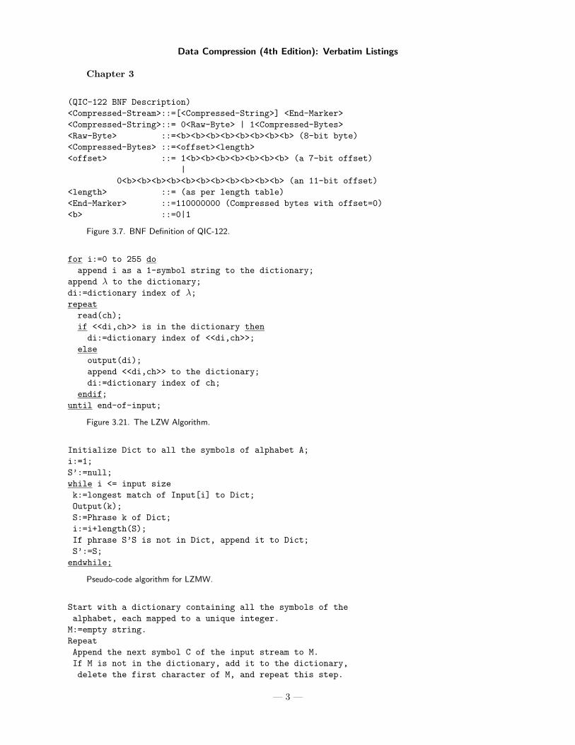
Figure 3.7. BNF Definition of QIC-122.

for i:=0 to 255 doappend i as a 1-symbol string to the dictionary;

append λ to the dictionary;di:=dictionary index of λ;repeatread(ch);if <<di,ch>> is in the dictionary thendi:=dictionary index of <<di,ch>>;

elseoutput(di);append <<di,ch>> to the dictionary;di:=dictionary index of ch;

endif;until end-of-input;

Figure 3.21. The LZW Algorithm.

Initialize Dict to all the symbols of alphabet A;i:=1;S’:=null;while i <= input sizek:=longest match of Input[i] to Dict;Output(k);S:=Phrase k of Dict;i:=i+length(S);If phrase S’S is not in Dict, append it to Dict;S’:=S;endwhile;

Pseudo-code algorithm for LZMW.

Start with a dictionary containing all the symbols of thealphabet, each mapped to a unique integer.M:=empty string.RepeatAppend the next symbol C of the input stream to M.If M is not in the dictionary, add it to the dictionary,delete the first character of M, and repeat this step.

— 3 —


Until end-of-input.

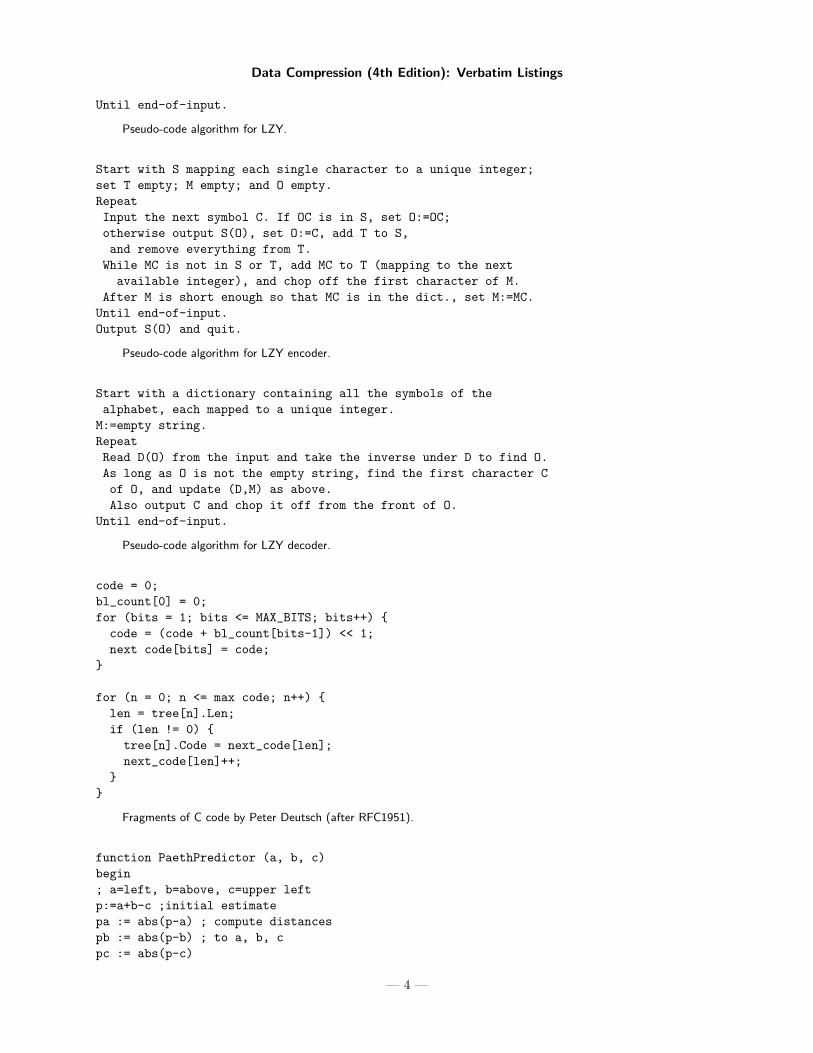
Pseudo-code algorithm for LZY.

Start with S mapping each single character to a unique integer;set T empty; M empty; and O empty.RepeatInput the next symbol C. If OC is in S, set O:=OC;otherwise output S(O), set O:=C, add T to S,and remove everything from T.While MC is not in S or T, add MC to T (mapping to the nextavailable integer), and chop off the first character of M.

After M is short enough so that MC is in the dict., set M:=MC.Until end-of-input.Output S(O) and quit.

Pseudo-code algorithm for LZY encoder.

Start with a dictionary containing all the symbols of thealphabet, each mapped to a unique integer.M:=empty string.RepeatRead D(O) from the input and take the inverse under D to find O.As long as O is not the empty string, find the first character Cof O, and update (D,M) as above.Also output C and chop it off from the front of O.

Until end-of-input.

Pseudo-code algorithm for LZY decoder.

code = 0;bl_count[0] = 0;for (bits = 1; bits <= MAX_BITS; bits++) {code = (code + bl_count[bits-1]) << 1;next code[bits] = code;

}

for (n = 0; n <= max code; n++) {len = tree[n].Len;if (len != 0) {tree[n].Code = next_code[len];next_code[len]++;

}}

Fragments of C code by Peter Deutsch (after RFC1951).

function PaethPredictor (a, b, c)begin; a=left, b=above, c=upper leftp:=a+b-c ;initial estimatepa := abs(p-a) ; compute distancespb := abs(p-b) ; to a, b, cpc := abs(p-c)

— 4 —


; return nearest of a,b,c,; breaking ties in order a,b,c.if pa<=pb AND pa<=pc then return aelse if pb<=pc then return belse return cend

Pseudo-code for the PaethPredictor function.

<card xmlns="http://businesscard.org"><name>Melvin Schwartzkopf</name><title>Chief person, Monster Inc.</title><email>[email protected]</email><phone>(212)555-1414</phone><logo url="widget.gif"/><red_backgrnd/>

</card>

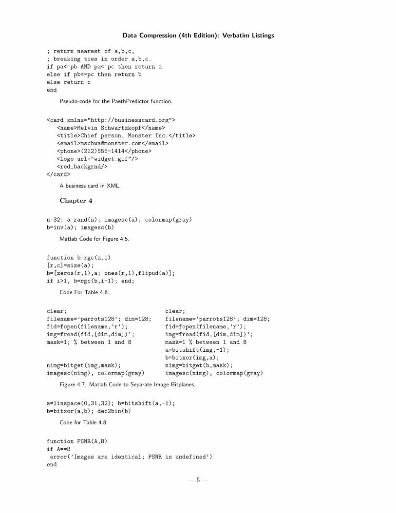
A business card in XML.

Chapter 4

n=32; a=rand(n); imagesc(a); colormap(gray)b=inv(a); imagesc(b)

Matlab Code for Figure 4.5.

function b=rgc(a,i)[r,c]=size(a);b=[zeros(r,1),a; ones(r,1),flipud(a)];if i>1, b=rgc(b,i-1); end;

Code For Table 4.6.

clear; clear;filename=’parrots128’; dim=128; filename=’parrots128’; dim=128;fid=fopen(filename,’r’); fid=fopen(filename,’r’);img=fread(fid,[dim,dim])’; img=fread(fid,[dim,dim])’;mask=1; % between 1 and 8 mask=1 % between 1 and 8

a=bitshift(img,-1);b=bitxor(img,a);

nimg=bitget(img,mask); nimg=bitget(b,mask);imagesc(nimg), colormap(gray) imagesc(nimg), colormap(gray)

Figure 4.7. Matlab Code to Separate Image Bitplanes.

a=linspace(0,31,32); b=bitshift(a,-1);b=bitxor(a,b); dec2bin(b)

Code for Table 4.8.

function PSNR(A,B)if A==Berror(’Images are identical; PSNR is undefined’)end

— 5 —


max2_A=max(max(A)); max2_B=max(max(B));min2_A=min(min(A)); min2_B=min(min(B));if max2_A>1 | max2_B>1 | min2_A<0 | min2_B<0

error(’pixels must be in [0,1]’)enddiffer=A-B;decib=20*log10(1/(sqrt(mean(mean(differ.^2)))));disp(sprintf(’PSNR = +%5.2f dB’,decib))

Figure 4.13. A Matlab Function to Compute PSNR.

p={{5,5},{6, 7},{12.1,13.2},{23,25},{32,29}};rot={{0.7071,-0.7071},{0.7071,0.7071}};Sum[p[[i,1]]p[[i,2]], {i,5}]q=p.rotSum[q[[i,1]]q[[i,2]], {i,5}]

Figure 4.15. Code For Rotating Five Points.

p=Table[Random[Real,{0,2}],{250}];p=Flatten[Append[p,Table[Random[Real,{1,3}],{250}]]];p=Flatten[Append[p,Table[Random[Real,{2,4}],{250}]]];p=Flatten[Append[p,Table[Random[Real,{3,5}],{250}]]];p=Flatten[Append[p,Table[Random[Real,{4,6}],{250}]]];p=Flatten[Append[p,Table[Random[Real,{0,6}],{150}]]];ListPlot[Table[{p[[i]],p[[i+1]]},{i,1,1399,2}]]

Mathematica code for Figure 4.16.

filename=’lena128’; dim=128;xdist=zeros(256,1); ydist=zeros(256,1);fid=fopen(filename,’r’);img=fread(fid,[dim,dim])’;for col=1:2:dim-1for row=1:dimx=img(row,col)+1; y=img(row,col+1)+1;xdist(x)=xdist(x)+1; ydist(y)=ydist(y)+1;endendfigure(1), plot(xdist), colormap(gray) %dist of x&y valuesfigure(2), plot(ydist), colormap(gray) %before rotationxdist=zeros(325,1); % clear arraysydist=zeros(256,1);for col=1:2:dim-1for row=1:dimx=round((img(row,col)+img(row,col+1))*0.7071);y=round((-img(row,col)+img(row,col+1))*0.7071)+101;xdist(x)=xdist(x)+1; ydist(y)=ydist(y)+1;endendfigure(3), plot(xdist), colormap(gray) %dist of x&y valuesfigure(4), plot(ydist), colormap(gray) %after rotation

Figure 4.17. Distribution of Image Pixels Before and After Rotation.

Needs["GraphicsImage‘"] (* Draws 2D Haar Coefficients *)n=8;h[k_,x_]:=Module[{p,q}, If[k==0, 1/Sqrt[n], (* h_0(x) *)p=0; While[2^p<=k ,p++]; p--; q=k-2^p+1; (* if k>0, calc. p, q *)

— 6 —


If[(q-1)/(2^p)<=x && x<(q-.5)/(2^p),2^(p/2),If[(q-.5)/(2^p)<=x && x<q/(2^p),-2^(p/2),0]]]];

HaarMatrix=Table[h[k,x], {k,0,7}, {x,0,7/n,1/n}] //N;HaarTensor=Array[Outer[Times, HaarMatrix[[#1]],HaarMatrix[[#2]]]&,{n,n}];Show[GraphicsArray[Map[GraphicsImage[#, {-2,2}]&, HaarTensor,{2}]]]

Code for Figure 4.20.

n=8;p={12.,10.,8.,10.,12.,10.,8.,11.};c=Table[If[t==1, 0.7071, 1], {t,1,n}];dct[i_]:=Sqrt[2/n]c[[i+1]]Sum[p[[t+1]]Cos[(2t+1)i Pi/16],{t,0,n-1}];q=Table[dct[i],{i,0,n-1}] (* use precise DCT coefficients *)q={28,0,0,2,3,-2,0,0}; (* or use quantized DCT coefficients *)idct[t_]:=Sqrt[2/n]Sum[c[[j+1]]q[[j+1]]Cos[(2t+1)j Pi/16],{j,0,n-1}];ip=Table[idct[t],{t,0,n-1}]

Figure 4.21. Experiments with the One-Dimensional DCT.

% 8x8 correlated valuesn=8;p=[00,10,20,30,30,20,10,00; 10,20,30,40,40,30,20,10; 20,30,40,50,50,40,30,20; ...30,40,50,60,60,50,40,30; 30,40,50,60,60,50,40,30; 20,30,40,50,50,40,30,20; ...10,20,30,40,40,30,12,10; 00,10,20,30,30,20,10,00];

figure(1), imagesc(p), colormap(gray), axis square, axis offdct=zeros(n,n);for j=0:7

for i=0:7for x=0:7

for y=0:7dct(i+1,j+1)=dct(i+1,j+1)+p(x+1,y+1)*cos((2*y+1)*j*pi/16)*cos((2*x+1)*i*pi/16);

end;end;

end;end;dct=dct/4; dct(1,:)=dct(1,:)*0.7071; dct(:,1)=dct(:,1)*0.7071;dctquant=[239,1,-90,0,0,0,0,0; 0,0,0,0,0,0,0,0; -90,0,0,0,0,0,0,0; 0,0,0,0,0,0,0,0; ...0,0,0,0,0,0,0,0; 0,0,0,0,0,0,0,0; 0,0,0,0,0,0,0,0; 0,0,0,0,0,0,0,0];

idct=zeros(n,n);for x=0:7

for y=0:7for i=0:7

if i==0 ci=0.7071; else ci=1; end;for j=0:7

if j==0 cj=0.7071; else cj=1; end;idct(x+1,y+1)=idct(x+1,y+1)+ ...

ci*cj*quant(i+1,j+1)*cos((2*y+1)*j*pi/16)*cos((2*x+1)*i*pi/16);end;

end;end;

end;idct=idct/4;idctfigure(2), imagesc(idct), colormap(gray), axis square, axis off

Figure 4.33. Code for Highly Correlated Pattern.

Table[N[t],{t,Pi/16,15Pi/16,Pi/8}]dctp[pw_]:=Table[N[Cos[pw t]],{t,Pi/16,15Pi/16,Pi/8}]dctp[0]dctp[1]...

— 7 —


dctp[7]

Code for Table 4.37.

dct[pw_]:=Plot[Cos[pw t], {t,0,Pi}, DisplayFunction->Identity,AspectRatio->Automatic];dcdot[pw_]:=ListPlot[Table[{t,Cos[pw t]},{t,Pi/16,15Pi/16,Pi/8}],DisplayFunction->Identity]Show[dct[0],dcdot[0], Prolog->AbsolutePointSize[4],DisplayFunction->$DisplayFunction]...Show[dct[7],dcdot[7], Prolog->AbsolutePointSize[4],DisplayFunction->$DisplayFunction]


dctp[fs_,ft_]:=Table[SetAccuracy[N[(1.-Cos[fs s]Cos[ft t])/2],3],{s,Pi/16,15Pi/16,Pi/8},{t,Pi/16,15Pi/16,Pi/8}]//TableFormdctp[0,0]dctp[0,1]...dctp[7,7]


Needs["GraphicsImage‘"] (* Draws 2D DCT Coefficients *)DCTMatrix=Table[If[k==0,Sqrt[1/8],Sqrt[1/4]Cos[Pi(2j+1)k/16]],{k,0,7}, {j,0,7}] //N;DCTTensor=Array[Outer[Times, DCTMatrix[[#1]],DCTMatrix[[#2]]]&,{8,8}];Show[GraphicsArray[Map[GraphicsImage[#, {-.25,.25}]&, DCTTensor,{2}]]]

Alternative Code for Figure 4.39.

DCTMatrix=Table[If[k==0,Sqrt[1/8],Sqrt[1/4]Cos[Pi(2j+1)k/16]],{k,0,7}, {j,0,7}] //N;DCTTensor=Array[Outer[Times, DCTMatrix[[#1]],DCTMatrix[[#2]]]&,{8,8}];img={{1,0,0,1,1,1,0,1},{1,1,0,0,1,0,1,1},{0,1,1,0,0,1,0,0},{0,0,0,1,0,0,1,0},{0,1,0,0,1,0,1,1},{1,1,1,0,0,1,1,0},{1,1,0,0,1,0,1,1},{0,1,0,1,0,0,1,0}};ShowImage[Reverse[img]]dctcoeff=Array[(Plus @@ Flatten[DCTTensor[[#1,#2]] img])&,{8,8}];dctcoeff=SetAccuracy[dctcoeff,4];dctcoeff=Chop[dctcoeff,.001];MatrixForm[dctcoeff]ShowImage[Reverse[dctcoeff]]


DCTMatrix=Table[If[k==0,Sqrt[1/8],Sqrt[1/4]Cos[Pi(2j+1)k/16]],{k,0,7}, {j,0,7}] //N;DCTTensor=Array[Outer[Times, DCTMatrix[[#1]],DCTMatrix[[#2]]]&,{8,8}];img={{0,1,0,1,0,1,0,1},{0,1,0,1,0,1,0,1},

— 8 —


{0,1,0,1,0,1,0,1},{0,1,0,1,0,1,0,1},{0,1,0,1,0,1,0,1},{0,1,0,1,0,1,0,1},{0,1,0,1,0,1,0,1},{0,1,0,1,0,1,0,1}};ShowImage[Reverse[img]]dctcoeff=Array[(Plus @@ Flatten[DCTTensor[[#1,#2]] img])&,{8,8}];dctcoeff=SetAccuracy[dctcoeff,4];dctcoeff=Chop[dctcoeff,.001];MatrixForm[dctcoeff]ShowImage[Reverse[dctcoeff]]


(* DCT-1. Notice (n+1)x(n+1) *)Clear[n, nor, kj, DCT1, T1];n=8; nor=Sqrt[2/n];kj[i_]:=If[i==0 || i==n, 1/Sqrt[2], 1];DCT1[k_]:=Table[nor kj[j] kj[k] Cos[j k Pi/n], {j,0,n}]T1=Table[DCT1[k], {k,0,n}]; (* Compute nxn cosines *)MatrixForm[T1] (* display as a matrix *)(* multiply rows to show orthonormality *)MatrixForm[Table[Chop[N[T1[[i]].T1[[j]]]], {i,1,n}, {j,1,n}]]

(* DCT-2 *)Clear[n, nor, kj, DCT2, T2];n=8; nor=Sqrt[2/n];kj[i_]:=If[i==0 || i==n, 1/Sqrt[2], 1];DCT2[k_]:=Table[nor kj[k] Cos[(j+1/2)k Pi/n], {j,0,n-1}]T2=Table[DCT2[k], {k,0,n-1}]; (* Compute nxn cosines *)MatrixForm[T2] (* display as a matrix *)(* multiply rows to show orthonormality *)MatrixForm[Table[Chop[N[T2[[i]].T2[[j]]]], {i,1,n}, {j,1,n}]]

(* DCT-3. This is the transpose of DCT-2 *)Clear[n, nor, kj, DCT3, T3];n=8; nor=Sqrt[2/n];kj[i_]:=If[i==0 || i==n, 1/Sqrt[2], 1];DCT3[k_]:=Table[nor kj[j] Cos[(k+1/2)j Pi/n], {j,0,n-1}]T3=Table[DCT3[k], {k,0,n-1}]; (* Compute nxn cosines *)MatrixForm[T3] (* display as a matrix *)(* multiply rows to show orthonormality *)MatrixForm[Table[Chop[N[T3[[i]].T3[[j]]]], {i,1,n}, {j,1,n}]]

(* DCT-4. This is DCT-1 shifted *)Clear[n, nor, DCT4, T4];n=8; nor=Sqrt[2/n];DCT4[k_]:=Table[nor Cos[(k+1/2)(j+1/2) Pi/n], {j,0,n-1}]T4=Table[DCT4[k], {k,0,n-1}]; (* Compute nxn cosines *)MatrixForm[T4] (* display as a matrix *)(* multiply rows to show orthonormality *)MatrixForm[Table[Chop[N[T4[[i]].T4[[j]]]], {i,1,n}, {j,1,n}]]

Figure 4.44. Code for Four DCT Types.

function [Q,R]=QRdecompose(A);% Computes the QR decomposition of matrix A

— 9 —


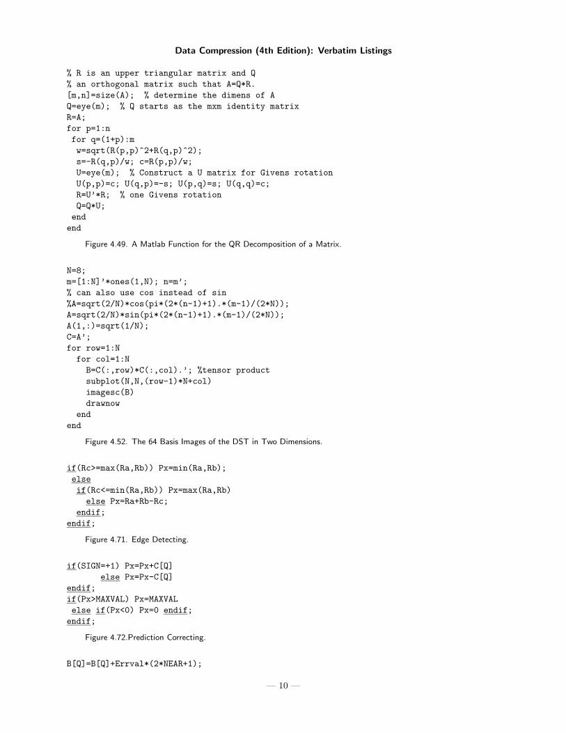
% R is an upper triangular matrix and Q% an orthogonal matrix such that A=Q*R.[m,n]=size(A); % determine the dimens of AQ=eye(m); % Q starts as the mxm identity matrixR=A;for p=1:nfor q=(1+p):mw=sqrt(R(p,p)^2+R(q,p)^2);s=-R(q,p)/w; c=R(p,p)/w;U=eye(m); % Construct a U matrix for Givens rotationU(p,p)=c; U(q,p)=-s; U(p,q)=s; U(q,q)=c;R=U’*R; % one Givens rotationQ=Q*U;endend

Figure 4.49. A Matlab Function for the QR Decomposition of a Matrix.

N=8;m=[1:N]’*ones(1,N); n=m’;% can also use cos instead of sin%A=sqrt(2/N)*cos(pi*(2*(n-1)+1).*(m-1)/(2*N));A=sqrt(2/N)*sin(pi*(2*(n-1)+1).*(m-1)/(2*N));A(1,:)=sqrt(1/N);C=A’;for row=1:Nfor col=1:NB=C(:,row)*C(:,col).’; %tensor productsubplot(N,N,(row-1)*N+col)imagesc(B)drawnow

endend

Figure 4.52. The 64 Basis Images of the DST in Two Dimensions.

if(Rc>=max(Ra,Rb)) Px=min(Ra,Rb);elseif(Rc<=min(Ra,Rb)) Px=max(Ra,Rb)else Px=Ra+Rb-Rc;

endif;endif;

Figure 4.71. Edge Detecting.

if(SIGN=+1) Px=Px+C[Q]else Px=Px-C[Q]

endif;if(Px>MAXVAL) Px=MAXVALelse if(Px<0) Px=0 endif;endif;

Figure 4.72.Prediction Correcting.

B[Q]=B[Q]+Errval*(2*NEAR+1);

— 10 —


A[Q]=A[Q]+abs(Errval);if(N[Q]=RESET) thenA[Q]=A[Q]>>1; B[Q]=B[Q]>>1; N[Q]=N[Q]>>1endif;N[Q]=N[Q]+1;

Figure 4.74. Updating Arrays A, B, and N .

RUNval=Ra;RUNcnt=0;while(abs(Ix-RUNval)<=NEAR)RUNcnt=RUNcnt+1;Rx=RUNval;if(EOLine=1) breakelse GetNextSample()endif;

endwhile;

Figure 4.75. Run Scanning.

while(RUNcnt>=(1<<J[RUNindex]))AppendToBitStream(1,1);RUNcnt=RUNcnt-(1<<J[RUNindex]);if(RUNindex<31)RUNindex=RUNindex+1;

endwhile;

Figure 4.76. Run Encoding: I.

if(EOLine=0) thenAppendToBitStream(0,1);AppendToBitStream(RUNcnt,J[RUNindex]);if(RUNindex>0)RUNindex=RUNindex-1;endif;else if(RUNcnt>0)AppendToBitStream(1,1);

Figure 4.77. Run Encoding: II.

for each level L dofor every pixel P in level L doCompute a prediction R for P using a group from level L-1;Compute E=R-P;Estimate the variance V to be used in encoding E;Quantize V and use it as an index to select a Laplace table LV;Use E as an index to table LV and retrieve LV[E];Use LV[E] as the probability to arithmetically encode E;endfor;Determine the pixels of the next level (rotate & scale);endfor;

Table 4.129. MLP Encoding.

— 11 —


Clear[Nh,P,U,W];Nh={{-4.5,13.5,-13.5,4.5},{9,-22.5,18,-4.5},{-5.5,9,-4.5,1},{1,0,0,0}};P={{p33,p32,p31,p30},{p23,p22,p21,p20},{p13,p12,p11,p10},{p03,p02,p01,p00}};U={u^3,u^2,u,1};W={w^3,w^2,w,1};u:=0.5;w:=0.5;Expand[U.Nh.P.Transpose[Nh].Transpose[W]]

Code to predict the value of a pixel as a polynomial interpolation of 16 of its near neighbors.

For all passesINITIALIZATION: N(d,t):=1; S(d,t):=0; d=0,1,...,L, t=0,1,...,2n;PARAMETERS: ak and wk are assigned their values;for all pixels x in the current pass do0: x =

∑nk=1 ak ·xk;

1: Δ =∑n

k=1 wk(xk − x);2: d = Quantize(Δ);3: Compute t = tn . . .t2t1;4: ε = S(d, t)/N(d, t);5: x = x + ε;6: ε = x − x;7: S(d, t) := S(d, t) + ε; N(d, t) := N(d, t) + 1;8: if N(d, t) ≥ 128 then

S(d, t) := S(d, t)/2; N(d, t) := N(d, t)/2;9: if S(d, t) < 0 encode(−ε, d) else encode(ε, d);endfor;end.

The CALIC encoder.

S=Table[N[Sin[t Degree]], {t,0,360,15}]Table[S[[i+1]]-S[[i]], {i,1,24}]


a={90.,95,100,80,90,85,75,96,91};b1={100,90,95,102,80,90,105,75,96};b2={101,128,108,100,90,95,102,80,90};b3={128,108,110,90,95,100,80,90,85};Solve[{b1.(a-w1 b1-w2 b2-w3 b3)==0,b2.(a-w1 b1-w2 b2-w3 b3)==0,b3.(a-w1 b1-w2 b2-w3 b3)==0},{w1,w2,w3}]

Figure 4.139. Solving for Three Weights.

x:=0; y:=0;for k:= n − 1 step −1 to 0 doif digit(k)=1 or 3 then y := y + 2k;if digit(k)=2 or 3 then x := x + 2k

endfor;

Figure 4.150. Pseudo-Code to Locate a Pixel in an Image.

— 12 —


/* Definitions:encode( value , min , max ); - function of encoding of value(output bits stream),min<=value<=max, the length of code is Log2(max-min+1) bits;Log2(N) - depth of pixel level of quadtree.struct knot_descriptor{int min,max; //min,max of the whole sub-planeint pix ; // value of pixel (in case of pixel level)int depth ; // depth of knot.knot_descriptor *square[4];//children’s sub-planes} ;Compact_quadtree (...) - recursive procedure of quadtree compression.*/Compact_quadtree (knot_descriptor *knot, int min, int max){encode( knot->min , min , max ) ;encode( knot->max , min , max ) ;if ( knot->min == knot->max ) return ;min = knot->min ;max= knot->max ;if ( knot->depth < Log2(N) ){Compact_quadtree(knot->square[ 0 ],min,max) ;Compact_quadtree(knot->square[ 1 ],min,max) ;Compact_quadtree(knot->square[ 2 ],min,max) ;Compact_quadtree(knot->square[ 3 ],min,max) ;}else{ // knot->depth == Log2(N) e pixel levelint slc = 0 ;encode( (knot->square[ 0 ])->pix , min , max );if ((knot->square[ 0 ])->pix == min) slc=1;else if ((knot->square[ 0 ])->pix==max) slc=2;encode( (knot->square[ 1 ])->pix , min , max );if ((knot->square[ 1 ])->pix == min) slc |= 1;else if ((knot->square[ 1 ])->pix==max) slc |= 2;switch( slc ){case 0:encode(((knot->square[2])->pix==max),0,1);return ;case 1:if ((knot->square[2])->pix==max){encode(1,0,1);encode((knot->square[ 3 ])->pix,min,max);}else{encode(0,0,1);encode((knot->square[ 2 ])->pix,min,max);}return ;case 2:if ((knot->square[2])->pix==min){encode(1,0,1);encode((knot->square[ 3 ])->pix,min,max);}else{encode(0,0,1);encode((knot->square[ 2 ])->pix,min,max);}return ;case 3:encode((knot->square[ 2 ])->pix,min,max);encode((knot->square[ 3 ])->pix,min,max);}}}

— 13 —


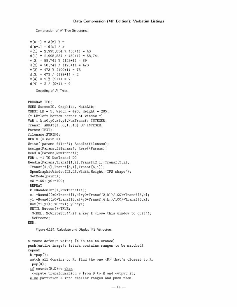
Compression of N -Tree Structures.

v[n+1] = d[n] % rd[n+1] = d[n] / rv[1] = 2,995,834 % (50+1) = 43d[1] = 2,995,834 / (50+1) = 58,741v[2] = 58,741 % (123+1) = 89d[2] = 58,741 / (123+1) = 473v[3] = 473 % (199+1) = 73d[3] = 473 / (199+1) = 2v[4] = 2 % (9+1) = 2d[4] = 2 / (9+1) = 0

Decoding of N -Trees.

PROGRAM IFS;USES ScreenIO, Graphics, MathLib;CONST LB = 5; Width = 490; Height = 285;(* LB=left bottom corner of window *)VAR i,k,x0,y0,x1,y1,NumTransf: INTEGER;Transf: ARRAY[1..6,1..10] OF INTEGER;Params:TEXT;filename:STRING;BEGIN (* main *)Write(’params file=’); Readln(filename);Assign(Params,filename); Reset(Params);Readln(Params,NumTransf);FOR i:=1 TO NumTransf DOReadln(Params,Transf[1,i],Transf[2,i],Transf[3,i],Transf[4,i],Transf[5,i],Transf[6,i]);OpenGraphicWindow(LB,LB,Width,Height,’IFS shape’);SetMode(paint);x0:=100; y0:=100;REPEATk:=RandomInt(1,NumTransf+1);x1:=Round((x0*Transf[1,k]+y0*Transf[2,k])/100)+Transf[5,k];y1:=Round((x0*Transf[3,k]+y0*Transf[4,k])/100)+Transf[6,k];Dot(x1,y1); x0:=x1; y0:=y1;UNTIL Button()=TRUE;ScBOL; ScWriteStr(’Hit a key & close this window to quit’);ScFreeze;

END.

Figure 4.184. Calculate and Display IFS Attractors.

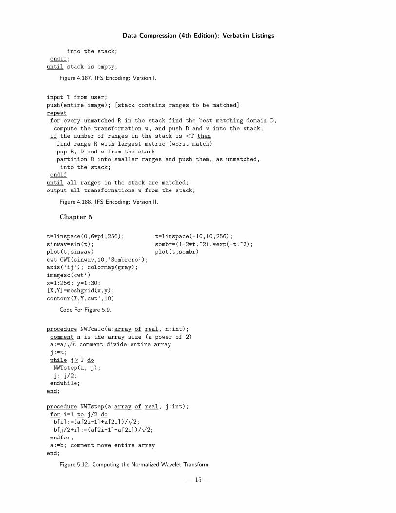
t:=some default value; [t is the tolerance]push(entire image); [stack contains ranges to be matched]repeatR:=pop();match all domains to R, find the one (D) that’s closest to R,pop(R);if metric(R,D)<t thencompute transformation w from D to R and output it;else partition R into smaller ranges and push them

— 14 —


into the stack;endif;

until stack is empty;

Figure 4.187. IFS Encoding: Version I.

input T from user;push(entire image); [stack contains ranges to be matched]repeatfor every unmatched R in the stack find the best matching domain D,compute the transformation w, and push D and w into the stack;if the number of ranges in the stack is <T thenfind range R with largest metric (worst match)pop R, D and w from the stackpartition R into smaller ranges and push them, as unmatched,into the stack;

endifuntil all ranges in the stack are matched;output all transformations w from the stack;

Figure 4.188. IFS Encoding: Version II.

Chapter 5

t=linspace(0,6*pi,256); t=linspace(-10,10,256);sinwav=sin(t); sombr=(1-2*t.^2).*exp(-t.^2);plot(t,sinwav) plot(t,sombr)cwt=CWT(sinwav,10,’Sombrero’);axis(’ij’); colormap(gray);imagesc(cwt’)x=1:256; y=1:30;[X,Y]=meshgrid(x,y);contour(X,Y,cwt’,10)

Code For Figure 5.9.

procedure NWTcalc(a:array of real, n:int);comment n is the array size (a power of 2)a:=a/

√n comment divide entire array

j:=n;while j≥ 2 doNWTstep(a, j);j:=j/2;endwhile;end;

procedure NWTstep(a:array of real, j:int);for i=1 to j/2 dob[i]:=(a[2i-1]+a[2i])/

√2;

b[j/2+i]:=(a[2i-1]-a[2i])/√

2;endfor;a:=b; comment move entire arrayend;

Figure 5.12. Computing the Normalized Wavelet Transform.

— 15 —


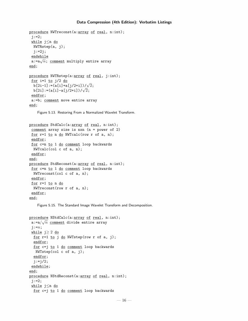
procedure NWTreconst(a:array of real, n:int);j:=2;while j≤n doNWTRstep(a, j);j:=2j;endwhilea:=a

√n; comment multiply entire array

end;

procedure NWTRstep(a:array of real, j:int);for i=1 to j/2 dob[2i-1]:=(a[i]+a[j/2+i])/

√2;

b[2i]:=(a[i]-a[j/2+i])/√

2;endfor;a:=b; comment move entire arrayend;

Figure 5.13. Restoring From a Normalized Wavelet Transform.

procedure StdCalc(a:array of real, n:int);comment array size is nxn (n = power of 2)for r=1 to n do NWTcalc(row r of a, n);endfor;for c=n to 1 do comment loop backwardsNWTcalc(col c of a, n);endfor;

end;procedure StdReconst(a:array of real, n:int);for c=n to 1 do comment loop backwardsNWTreconst(col c of a, n);endfor;for r=1 to n doNWTreconst(row r of a, n);endfor;end;

Figure 5.15. The Standard Image Wavelet Transform and Decomposition.

procedure NStdCalc(a:array of real, n:int);a:=a/

√n comment divide entire array

j:=n;while j≥ 2 dofor r=1 to j do NWTstep(row r of a, j);endfor;for c=j to 1 do comment loop backwardsNWTstep(col c of a, j);endfor;j:=j/2;endwhile;end;procedure NStdReconst(a:array of real, n:int);j:=2;while j≤n dofor c=j to 1 do comment loop backwards

— 16 —


NWTRstep(col c of a, j);endfor;for r=1 to j doNWTRstep(row r of a, j);endfor;j:=2j;endwhilea:=a

√n; comment multiply entire array

end;

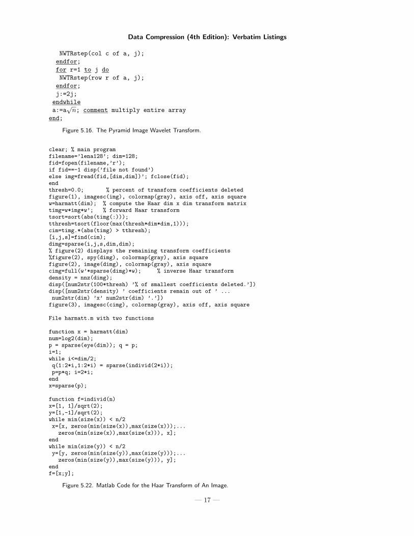
Figure 5.16. The Pyramid Image Wavelet Transform.

clear; % main programfilename=’lena128’; dim=128;fid=fopen(filename,’r’);if fid==-1 disp(’file not found’)else img=fread(fid,[dim,dim])’; fclose(fid);endthresh=0.0; % percent of transform coefficients deletedfigure(1), imagesc(img), colormap(gray), axis off, axis squarew=harmatt(dim); % compute the Haar dim x dim transform matrixtimg=w*img*w’; % forward Haar transformtsort=sort(abs(timg(:)));tthresh=tsort(floor(max(thresh*dim*dim,1)));cim=timg.*(abs(timg) > tthresh);[i,j,s]=find(cim);dimg=sparse(i,j,s,dim,dim);% figure(2) displays the remaining transform coefficients%figure(2), spy(dimg), colormap(gray), axis squarefigure(2), image(dimg), colormap(gray), axis squarecimg=full(w’*sparse(dimg)*w); % inverse Haar transformdensity = nnz(dimg);disp([num2str(100*thresh) ’% of smallest coefficients deleted.’])disp([num2str(density) ’ coefficients remain out of ’ ...num2str(dim) ’x’ num2str(dim) ’.’])figure(3), imagesc(cimg), colormap(gray), axis off, axis square

File harmatt.m with two functions

function x = harmatt(dim)num=log2(dim);p = sparse(eye(dim)); q = p;i=1;while i<=dim/2;q(1:2*i,1:2*i) = sparse(individ(2*i));p=p*q; i=2*i;endx=sparse(p);

function f=individ(n)x=[1, 1]/sqrt(2);y=[1,-1]/sqrt(2);while min(size(x)) < n/2x=[x, zeros(min(size(x)),max(size(x)));...zeros(min(size(x)),max(size(x))), x];

endwhile min(size(y)) < n/2y=[y, zeros(min(size(y)),max(size(y)));...zeros(min(size(y)),max(size(y))), y];

endf=[x;y];

Figure 5.22. Matlab Code for the Haar Transform of An Image.

— 17 —


function wc1=fwt1(dat,coarse,filter)% The 1D Forward Wavelet Transform% dat must be a 1D row vector of size 2^n,% coarse is the coarsest level of the transform% (note that coarse should be <<n)% filter is an orthonormal quadrature mirror filter% whose length should be <2^(coarse+1)n=length(dat); j=log2(n); wc1=zeros(1,n);beta=dat;for i=j-1:-1:coarsealfa=HiPass(beta,filter);wc1((2^(i)+1):(2^(i+1)))=alfa;beta=LoPass(beta,filter) ;

endwc1(1:(2^coarse))=beta;

function d=HiPass(dt,filter) % highpass downsamplingd=iconv(mirror(filter),lshift(dt));% iconv is matlab convolution tooln=length(d);d=d(1:2:(n-1));

function d=LoPass(dt,filter) % lowpass downsamplingd=aconv(filter,dt);% aconv is matlab convolution tool with time-% reversal of filtern=length(d);d=d(1:2:(n-1));

function sgn=mirror(filt)% return filter coefficients with alternating signssgn=-((-1).^(1:length(filt))).*filt;

Code for Function fwt1.

function dat=iwt1(wc,coarse,filter)% Inverse Discrete Wavelet Transformdat=wc(1:2^coarse);n=length(wc); j=log2(n);for i=coarse:j-1dat=ILoPass(dat,filter)+ ...IHiPass(wc((2^(i)+1):(2^(i+1))),filter);

end

function f=ILoPass(dt,filter)f=iconv(filter,AltrntZro(dt));

function f=IHiPass(dt,filter)f=aconv(mirror(filter),rshift(AltrntZro(dt)));


function f=AltrntZro(dt)% returns a vector of length 2*n with zeros% placed between consecutive valuesn =length(dt)*2; f =zeros(1,n);f(1:2:(n-1))=dt;

Figure 5.32: Code for the One-Dimensional Inverse Discrete Wavelet Transform.

function wc=fwt2(dat,coarse,filter)% The 2D Forward Wavelet Transform

— 18 —


% dat must be a 2D matrix of size (2^n:2^n),% "coarse" is the coarsest level of the transform% (note that coarse should be <<n)% filter is an orthonormal qmf of length<2^(coarse+1)q=size(dat); n = q(1); j=log2(n);if q(1)~=q(2), disp(’Nonsquare image!’), end;wc = dat; nc = n;for i=j-1:-1:coarse,top = (nc/2+1):nc; bot = 1:(nc/2);for ic=1:nc,row = wc(ic,1:nc);wc(ic,bot)=LoPass(row,filter);wc(ic,top)=HiPass(row,filter);endfor ir=1:nc,row = wc(1:nc,ir)’;wc(top,ir)=HiPass(row,filter)’;wc(bot,ir)=LoPass(row,filter)’;endnc = nc/2;end

function d=HiPass(dt,filter) % highpass downsamplingd=iconv(mirror(filter),lshift(dt));% iconv is matlab convolution tooln=length(d);d=d(1:2:(n-1));

function d=LoPass(dt,filter) % lowpass downsamplingd=aconv(filter,dt);% aconv is matlab convolution tool with time-% reversal of filtern=length(d);d=d(1:2:(n-1));


Function fwt2.

filename=’house128’; dim=128;fid=fopen(filename,’r’);if fid==-1 disp(’file not found’)else img=fread(fid,[dim,dim])’; fclose(fid);endfilt=[0.4830 0.8365 0.2241 -0.1294];fwim=fwt2(img,4,filt);figure(1), imagesc(fwim), axis off, axis squarerec=iwt2(fwim,4,filt);figure(2), imagesc(rec), axis off, axis square

Test of Function fwt2.

function dat=iwt2(wc,coarse,filter)% Inverse Discrete 2D Wavelet Transformn=length(wc); j=log2(n);dat=wc;nc=2^(coarse+1);for i=coarse:j-1,top=(nc/2+1):nc; bot=1:(nc/2); all=1:nc;for ic=1:nc,dat(all,ic)=ILoPass(dat(bot,ic)’,filter)’ ...+IHiPass(dat(top,ic)’,filter)’;

— 19 —


end % icfor ir=1:nc,dat(ir,all)=ILoPass(dat(ir,bot),filter) ...+IHiPass(dat(ir,top),filter);

end % irnc=2*nc;end % i





Figure 5.34, Function iwt2

filename=’house128’; dim=128;fid=fopen(filename,’r’);if fid==-1 disp(’file not found’)else img=fread(fid,[dim,dim])’; fclose(fid);endfilt=[0.4830 0.8365 0.2241 -0.1294];fwim=fwt2(img,4,filt);figure(1), imagesc(fwim), axis off, axis squarerec=iwt2(fwim,4,filt);figure(2), imagesc(rec), axis off, axis square

A test of fwt2 and iwt2.

clear, colormap(gray);filename=’lena128’; dim=128;fid=fopen(filename,’r’);img=fread(fid,[dim,dim])’;filt=[0.23037,0.71484,0.63088,-0.02798, ...-0.18703,0.03084,0.03288,-0.01059];fwim=fwt2(img,3,filt);figure(1), imagesc(fwim), axis squarefwim(1:16,17:32)=fwim(1:16,17:32)/2;fwim(1:16,33:128)=0;fwim(17:32,1:32)=fwim(17:32,1:32)/2;fwim(17:32,33:128)=0;fwim(33:128,:)=0;figure(2), colormap(gray), imagesc(fwim)rec=iwt2(fwim,3,filt);figure(3), colormap(gray), imagesc(rec)

Code For Figure Ans.54.

function multres(wc,coarse,filter)% A multi resolution plot of a 1D wavelet transformscale=1./max(abs(wc));n=length(wc); j=log2(n);LockAxes([0 1 -(j) (-coarse+2)]);t=(.5:(n-.5))/n;

— 20 —


for i=(j-1):-1:coarsez=zeros(1,n);z((2^(i)+1):(2^(i+1)))=wc((2^(i)+1):(2^(i+1)));dat=iwt1(z,i,filter);plot(t,-(i)+scale.*dat);endz=zeros(1,n);z(1:2^(coarse))=wc(1:2^(coarse));dat=iwt1(z,coarse,filter);plot(t,(-(coarse-1))+scale.*dat);UnlockAxes;

a test routine

n=1024; t=(1:n)./n;dat=spikes(t); % several spikes%p=floor(n*.37); dat=1./abs(t-(p+.5)/n); % one spikefigure(1), plot(t,dat)filt=[0.4830 0.8365 0.2241 -0.1294];wc=fwt1(dat,2,filt);figure(2), plot(t,wc)figure(3)multres(wc,2,filt);

function dat=spikes(t)pos=[.05 .11 .14 .22 .26 .41 .44 .64 .77 .79 .82];hgt=[5 5 4 4.5 5 3.9 3.3 4.6 1.1 5 4];wth=[.005 .005 .006 .01 .01 .03 .01 .01 .005 .008 .005];dat=zeros(size(t));for i=1:length(pos)dat=dat+hgt(i)./(1+abs((t-pos(i))./wth(i))).^4;end;

Figure 5.39. Matlab Code for the Multiresolution Decomposition of a One-Dimensional Row Vector.

1. Initialization:Initialize LP with all Ci,j in LFS,Initialize LIS with all parent nodes,Output n = �log2(max |Ci,j |/q)�.Set the threshold T = q2n, where q is a quality factor.

2. Sorting:for each node k in LIS dooutput ST (k)if ST (k) = 1 thenfor each child of k domove coefficients to LPadd to LIS as a new nodeendforremove k from LIS

endifendfor

3. Quantization: For each element in LP,quantize and encode using ACTCQ.(use TCQ step size Δ = α · q).

4. Update: Remove all elements in LP. Set T = T/2. Go to step 2.

Figure 5.61. QTCQ Encoding.

Chapter 7

— 21 —


% File ’LaplaceWav.m’filename=’a8.wav’;dim=2950; % size of file a8.wavdist=zeros(256,1); ddist=zeros(512,1);fid=fopen(filename,’r’);buf=fread(fid,dim,’uint8’); %input unsigned integersfor i=46:dim % skip .wav file headerx=buf(i)+1; dif=buf(i)-buf(i-1)+256;dist(x)=dist(x)+1; ddist(dif)=ddist(dif)+1;endfigure(1), plot(dist), colormap(gray) %dist of audio samplesfigure(2), plot(ddist), colormap(gray) %dist of differencesdist=zeros(256,1); ddist=zeros(512,1); % clear buffersbuf=randint(dim,1,[0 255]); % many random numbersfor i=2:dimx=buf(i)+1; dif=buf(i)-buf(i-1)+256;dist(x)=dist(x)+1; ddist(dif)=ddist(dif)+1;endfigure(3), plot(dist), colormap(gray) %dist of random numbersfigure(4), plot(ddist), colormap(gray) %dist of differences

Code For Figure 7.4.

dat=linspace(0,1,1000);mu=255;plot(dat*8159,128*log(1+mu*dat)/log(1+mu));

Matlab code for Figure 7.12.

(* Uniform Cubic Lagrange polynomial for 4th-order prediction in FLAC *)Clear[Q,t]; t0=0; t1=1; t2=2; t3=3;Q[t_] := Plus @@ {((t-t1)(t-t2)(t-t3))/((t0-t1)(t0-t2)(t0-t3))P4,((t-t0)(t-t2)(t-t3))/((t1-t0)(t1-t2)(t1-t3))P3,((t-t0)(t-t1)(t-t3))/((t2-t0)(t2-t1)(t2-t3))P2,((t-t0)(t-t1)(t-t2))/((t3-t0)(t3-t1)(t3-t2))P1}

Figure 7.30. Code For a Lagrange Polynomial.

for first audio frame:rest:=0;padding:=no;

for each subsequent audio frame:if layer=Ithen dif:=(12 × bitrate) modulo (sampling-frequency)else dif:=(144 × bitrate) modulo (sampling-frequency);

rest:=rest−dif;if rest<0 then

padding:=yes;rest:=rest+(sampling-frequency)

else padding:=no;

Algorithm used by the mp3 encoder to determine whether or not padding is necessary.

if (unsigned) {mod = lav + 1;off = 0;

}else {

— 22 —


mod = 2*lav + 1;off = lav;

}if (dim == 4) {w = INT(idx/(mod*mod*mod)) - off;idx -= (w+off)*(mod*mod*mod)x = INT(idx/(mod*mod)) - off;idx -= (x+off)*(mod*mod)y = INT(idx/mod) - off;idx -= (y+off)*modz = idx - off;

}else {y = INT(idx/mod) - off;idx -= (y+off)*modz = idx - off;

}

Figure 7.81. Decoding Frequency Coefficients in AAC.

Chapter 8

Input the first item. This is a raw symbol. Output it.while not end-of-fileInput the next item. This is the rank of a symbol.If this rank is > the total number of distinct symbols seen so farthen Input the next item. This is a raw symbol. Output it.else Translate the rank into a symbol using the current

context ranking. Output this symbol.endifThe string that has been output so far is the current context.Insert it into the table of sorted contexts.

endwhile

Figure 8.17. The Decoding Algorithm of Section 8.4.

Clear[t]; t=Log[4]; (* natural log *)Table[{n,N[0.5 Log[2,4^n/(n t)],3]}, {n,1,12}]//TableForm

Mathematica Code for Table 8.27.

procedure RowCol(ind,R1,R2,C1,C2: integer);case ind of0: R2:=(R1+R2)÷2; C2:=(C1+C2)÷2;1: R2:=(R1+R2)÷2; C1:=((C1+C2)÷2) + 1;2: R1:=((R1+R2)÷2) + 1; C2:=(C1+C2)÷2;3: R1:=((R1+R2)÷2) + 1; C1:=((C1+C2)÷2) + 1;endcase;if ind≤n then RowCol(ind+1,R1,R2,C1,C2);end RowCol;

main programinteger ind, R1, R2, C1, C2;integer array id[10];bit array M[2n, 2n];ind:=0; R1:=0; R2:=2n − 1; C1:=0; C2:=2n − 1;

— 23 —


RowCol(ind, R1, R2, C1, C2);M[R1,C1]:=1;end;

Figure 8.28. Recursive Procedure RowCol (Section 8.5.5).

procedure RowCol(ind,R1,R2,C1,C2: integer);case ind of0: R2:=(R1+R2)÷2; C2:=(C1+C2)÷2;1: R2:=(R1+R2)÷2; C1:=((C1+C2)÷2) + 1;2: R1:=((R1+R2)÷2) + 1; C2:=(C1+C2)÷2;3: R1:=((R1+R2)÷2) + 1; C1:=((C1+C2)÷2) + 1;endcase;if ind≤n then RowCol(ind+1,R1,R2,C1,C2);end RowCol;

main programinteger ind, R1, R2, C1, C2;integer array id[10];bit array M[2n, 2n];ind:=0; R1:=0; R2:=2n − 1; C1:=0; C2:=2n − 1;RowCol(ind, R1, R2, C1, C2);M[R1,C1]:=1;end;

Figure 8.28. Recursive Procedure RowCol.

repeatinput an alphanumeric word W;if W is in the A-tree thenoutput code of W;increment count of W;elseoutput an A-escape;output W (perhaps coded);add W to the A-tree with a count of 1;Increment the escape countendif;rearrange the A-tree if necessary;input an ‘‘other’’ word P;if P is in the P-tree then...... code similar to the above...until end-of-file.

Figure 8.29. Word-Based Adaptive Huffman Algorithm.

S:=empty string;repeatif currentIsAlph then input alphanumeric word W

else input non-alphanumeric word W;endif;if W is a new word then

— 24 —


if S is not the empty string then output string # of S; endif;output an escape followed by the text of W;S:=empty string;elseif startIsAlph then search A-dictionary for string S,W

else search P-dictionary for string S,W;endif;if S,W was found then S:=S,Welseoutput string numer of S;add S to either the A- or the P-dictionary;startIsAlph:=currentIsAlph;S:=W;

endif;endif;currentIsAlph:=not currentIsAlph;until end-of-file.

Figure 8.30. Word-Based LZW.

prevW:=escape;repeatinput next punctuation word WP and output its text;input next alphanumeric word WA;if WA is new thenoutput an escape;output WA arithmetically encoded by characters;add AW to list of words;set frequency of pair (prevW,WA) to 1;increment frequency of the pair (prevW,escape) by 1;elseoutput WA arithmetically encoded;increment frequency of the pair (prevW,WA);endif;prevW:=WA;until end-of-file.

Figure 8.31. Word-Based Order-1 Predictor.

H=H|E; % append E to historyg.m=0; g.n.m=0; g.p.m=0; % unmark edgesif StackEmpty then stopelse PopStack; g=StackTop;% start on next regionendif

Figure 8.45. Handling Case E of Edgebreaker.

H=H|C; % append C to historyP=P|g.v; % append v to Pg.m=0; g.p.o.m=1; % update flagsg.n.o.m=1; g.v.m=1;g.p.o.P=g.P; g.P.N=g.p.o; % fix link 1g.p.o.N=g.n.o; g.n.o.P=g.p.o; % fix link 2g.n.o.N=g.N; g.N.P=g.n.o; % fix link 3g=g.n.o; StackTop=g; % advance gate

— 25 —


Figure 8.46. Handling Case C of Edgebreaker.

H=H|L; % append L to historyg.m=0; g.P.m=0; g.n.o.m=1; % update flagsg.P.P.n=g.n.o; g.n.o.P=g.P.P; % fix link 1g.n.o.N=g.N; g.N.P=g.n.o; % fix link 2g=g.n.o; StackTop=g; % advance gate

Figure 8.47. Handling Case L of Edgebreaker.

H=H|R; % append R to historyg.m=0; g.N.m=0; g.p.o.m=1; % update flagsg.N.N.P=g.p.o; g.p.o.N=g.N.N. % fix link 1g.p.o.P=g.P; g.P.N=g.p.o; % fix link 2g=g.p.o; StackTop=g; % advance gate

Figure 8.48. Handling Case R of Edgebreaker.

H=H|S; % append S to historyg.m=0; g.n.o.m=1; g.p.o.m=1; % update flagsb=g.n; % initial candidate for bwhile not b.m do b=b.o.p;

% turn around v to marked bg.P.N=g.p.o; g.p.o.P=g.P. % fix link 1g.p.o.N=b.N; b.N.P=g.p.o; % fix link 2b.N=g.n.o; g.n.o.P=b; % fix link 3g.n.o.N=g.N; g.N.P=g.n.o; % fix link 4StackTop=g.p.o; PushStack; % save new regiong=g.n.o; StackTop=g; % advance gate

Figure 8.49. Handling Case S of Edgebreaker.

(* 3D DCT for hyperspectral data *)Clear[Pixl, DCT];Cr[i_]:=If[i==0,1/Sqrt[2],1];DCT[i_,j_,k_]:=(Sqrt[2]/32) Cr[i]Cr[j]Cr[k]Sum[Pixl[[x+1,y+1,z+1]]Cos[(2x+1)i Pi/8]Cos[(2y+1)j Pi/8]Cos[(2z+1)k Pi/8],{x, 0, 3}, {y, 0, 3}, {z, 0, 3}];Pixl = Table[Random[Integer, {30, 60}],{4},{4},{4}];Table[Round[DCT[m,n,p]],{m,0,3},{n,0,3},{p,0,3}];MatrixForm[%]

Figure 8.62. Three-Dimensional DCT Applied to Correlated Data.

Answers to exercises

a=rand(32); b=inv(a);figure(1), imagesc(a), colormap(gray); axis squarefigure(2), imagesc(b), colormap(gray); axis squarefigure(3), imagesc(cov(a)), colormap(gray); axis squarefigure(4), imagesc(cov(b)), colormap(gray); axis square

Code for Figure Ans.28.

a=linspace(0,31,32); b=bitshift(a,-1);b=bitxor(a,b); dec2bin(b)

Code For Table Ans.29.

— 26 —


M=3; N=2^M; H=[1 1; 1 -1]/sqrt(2);for m=1:(M-1) % recursionH=[H H; H -H]/sqrt(2);

endA=H’;map=[1 5 7 3 4 8 6 2]; % 1:Nfor n=1:N, B(:,n)=A(:,map(n)); end;A=B;sc=1/(max(abs(A(:))).^2); % scale factorfor row=1:Nfor col=1:NBI=A(:,row)*A(:,col).’; % tensor productsubplot(N,N,(row-1)*N+col)oe=round(BI*sc); % results in -1, +1imagesc(oe), colormap([1 1 1; .5 .5 .5; 0 0 0])drawnow

endend

Matlab Code for Figure Ans.31.

Clear[Nh,p,pnts,U,W];p00={0,0,0}; p10={1,0,1}; p20={2,0,1}; p30={3,0,0};p01={0,1,1}; p11={1,1,2}; p21={2,1,2}; p31={3,1,1};p02={0,2,1}; p12={1,2,2}; p22={2,2,2}; p32={3,2,1};p03={0,3,0}; p13={1,3,1}; p23={2,3,1}; p33={3,3,0};Nh={{-4.5,13.5,-13.5,4.5},{9,-22.5,18,-4.5},{-5.5,9,-4.5,1},{1,0,0,0}};pnts={{p33,p32,p31,p30},{p23,p22,p21,p20},{p13,p12,p11,p10},{p03,p02,p01,p00}};U[u_]:={u^3,u^2,u,1}; W[w_]:={w^3,w^2,w,1};(* prt [i] extracts component i from the 3rd dimen of P *)prt[i_]:=pnts[[Range[1,4],Range[1,4],i]];p[u_,w_]:={U[u].Nh.prt[1].Transpose[Nh].W[w],U[u].Nh.prt[2].Transpose[Nh].W[w], \U[u].Nh.prt[3].Transpose[Nh].W[w]};g1=ParametricPlot3D[p[u,w], {u,0,1},{w,0,1},Compiled->False, DisplayFunction->Identity];g2=Graphics3D[{AbsolutePointSize[2],Table[Point[pnts[[i,j]]],{i,1,4},{j,1,4}]}];Show[g1,g2, ViewPoint->{-2.576, -1.365, 1.718}]

Code For Figure Ans.37.

dim=256;for i=1:dimfor j=1:dimm(i,j)=(i+j-2)/(2*dim-2);

endendm

Figure Ans.45. Matlab Code for A Matrix mi,j = (i + j)/2.

cleara1=[1/2 1/2 0 0 0 0 0 0; 0 0 1/2 1/2 0 0 0 0;0 0 0 0 1/2 1/2 0 0; 0 0 0 0 0 0 1/2 1/2;1/2 -1/2 0 0 0 0 0 0; 0 0 1/2 -1/2 0 0 0 0;0 0 0 0 1/2 -1/2 0 0; 0 0 0 0 0 0 1/2 -1/2];% a1*[255; 224; 192; 159; 127; 95; 63; 32];a2=[1/2 1/2 0 0 0 0 0 0; 0 0 1/2 1/2 0 0 0 0;1/2 -1/2 0 0 0 0 0 0; 0 0 1/2 -1/2 0 0 0 0;

— 27 —


0 0 0 0 1 0 0 0; 0 0 0 0 0 1 0 0;0 0 0 0 0 0 1 0; 0 0 0 0 0 0 0 1];a3=[1/2 1/2 0 0 0 0 0 0; 1/2 -1/2 0 0 0 0 0 0;0 0 1 0 0 0 0 0; 0 0 0 1 0 0 0 0;0 0 0 0 1 0 0 0; 0 0 0 0 0 1 0 0;0 0 0 0 0 0 1 0; 0 0 0 0 0 0 0 1];w=a3*a2*a1;dim=8; fid=fopen(’8x8’,’r’);img=fread(fid,[dim,dim])’; fclose(fid);w*img*w’ % Result of the transform

Code for Figure Ans.52, Calculation of Matrix W and Transform W ·I ·WT .

function dat=iwt1(wc,coarse,filter)% Inverse Discrete Wavelet Transformdat=wc(1:2^coarse);n=length(wc); j=log2(n);for i=coarse:j-1dat=ILoPass(dat,filter)+ ...IHiPass(wc((2^(i)+1):(2^(i+1))),filter);

end





Figure Ans.53. Code For the 1D Inverse Discrete Wavelet Transform.

n=16; t=(1:n)./n;dat=sin(2*pi*t)filt=[0.4830 0.8365 0.2241 -0.1294];wc=fwt1(dat,1,filt)rec=iwt1(wc,1,filt)

Test of iwt1

Clear[p,a,b,c,d,e,f];p[t_]:=a t^5+b t^4+c t^3+d t^2+e t+f;Solve[{p[0]==p1, p[1/5.]==p2, p[2/5.]==p3,p[3/5.]==p4, p[4/5.]==p5, p[1]==p6}, {a,b,c,d,e,f}];sol=ExpandAll[Simplify[%]];Simplify[p[0.5] /.sol]

Figure Ans.55. Code for a Degree-5 Interpolating Polynomial.

clear;N=8; k=N/2;

— 28 —


x=[112,97,85,99,114,120,77,80];% Forward IWT into yfor i=0:k-2,y(2*i+2)=x(2*i+2)-floor((x(2*i+1)+x(2*i+3))/2);end;y(N)=x(N)-x(N-1);y(1)=x(1)+floor(y(2)/2);for i=1:k-1,y(2*i+1)=x(2*i+1)+floor((y(2*i)+y(2*i+2))/4);end;% Inverse IWT into zz(1)=y(1)-floor(y(2)/2);for i=1:k-1,z(2*i+1)=y(2*i+1)-floor((y(2*i)+y(2*i+2))/4);end;for i=0:k-2,z(2*i+2)=y(2*i+2)+floor((z(2*i+1)+x(2*i+3))/2);end;z(N)=y(N)+z(N-1);

Figure Ans.56. Matlab Code For Forward and Inverse IWT.

(* Points on a circle. Used in exercise to check4th-order prediction in FLAC *)r = 10;ci[x_] := Sqrt[100 - x^2];ci[0.32r]4ci[0] - 6ci[0.08r] + 4ci[0.16r] - ci[0.24r]

Figure Ans.57. Code For Checking 4th-Order Prediction.

[End of listings for the 4th edition.]

— 29 —

Documents

Data Compression, 4th Edition. Program and Pseudo … Compression, 4th Edition. Program and Pseudo-Code Listings (Advise the author about missing or bad listings.) Chapter 1 % Returns