Embed Size (px)
Citation preview
DATA DRIVEN MODEL DISCOVERY AND CONTROL OF LONGITUDINAL
MISSILE DYNAMICS
A THESIS SUBMITTED TO
THE GRADUATE SCHOOL OF NATURAL AND APPLIED SCIENCES
OF
MIDDLE EAST TECHNICAL UNIVERSITY
BY
HASAN MATPAN
IN PARTIAL FULFILLMENT OF THE REQUIREMENTS
FOR
THE DEGREE OF MASTER OF SCIENCE
IN
MECHANICAL ENGINEERING
SEPTEMBER 2021


Approval of the thesis:
DATA DRIVEN MODEL DISCOVERY AND CONTROL OF
LONGITUDINAL MISSILE DYNAMICS
submitted by HASAN MATPAN in partial fulfillment of the requirements for the
degree of Master of Science in Mechanical Engineering, Middle East Technical
University by,
Prof. Dr. Halil Kalıpçılar
Dean, Graduate School of Natural and Applied Sciences
Prof. Dr. M. A. Sahir Arıkan
Head of the Department, Mechanical Engineering
Assoc. Prof. Dr. A. Buğra Koku
Supervisor, Mechanical Engineering
Examining Committee Members:
Assoc. Prof. Dr. Yiğit Yazıcıoğlu
Mechanical Engineering, METU
Assoc. Prof. Dr. A. Buğra Koku
Mechanical Engineering, METU
Assoc. Prof. Dr. Mehmet Bülent Özer
Mechanical Engineering, METU
Assist. Prof. Dr. Ali Emre Turgut
Mechanical Engineering, METU
Prof. Dr. Duygun Erol Barkana
Electrical and Electronics Eng., Yeditepe Uni.
Date: 07.09.2021

iv
I hereby declare that all information in this document has been obtained and
presented in accordance with academic rules and ethical conduct. I also declare
that, as required by these rules and conduct, I have fully cited and referenced all
material and results that are not original to this work.
Name, Surname:
Signature:
Hasan Matpan
v
ABSTRACT
DATA DRIVEN MODEL DISCOVERY AND CONTROL OF
LONGITUDINAL MISSILE DYNAMICS
Matpan, Hasan
Master of Science, Mechanical Engineering
Supervisor: Assoc. Prof. Dr. A. Buğra Koku
September 2021, 105 pages
Dynamical systems in nature are generally nonlinear and usually contains many
hidden dynamics. Therefore, the need for data-driven model discovery and control
methods continues. The most popular of these methods is neural networks-based
methods nowadays. However, excessive data requirements, long training times and
most importantly lack of interpretability of results are the main problems in neural
networks-based system identification methods. Among the many other methods used
for model discovery, SINDY (Sparce Identification of Non-linear Dynamical
Systems) has recently attracted great attention with its simple and effective nature.
SINDY, which has many extensions, also has various open problems.
The proposed extension in this study is called SINDY-SAIC and combines the
methods from Stepwise Sparse Regression (SSR) and Akaike Information Criteria
(AIC) model selection algorithm. The need for tuning threshold parameter in SINDY
is relaxed using SSR and the robustness to noisy measurements is increased with a
newly used state derivative calculation method in sparse regression. In addition,
presence of model selection with AIC enables sparse solution by penalizing the
number of terms and prevents the algorithm to converge collinear basis.

vi
Studied dynamical systems are controlled by Model Predictive Control using
discovered models. MPC is a control method that uses prediction models mostly
discovered from data and try to minimize a given cost function subjected to the
constraints. Both linear and nonlinear prediction models are generated using SINDY-
SAIC and used in MPC as prediction models. The traditional state feedback (SF)
controller is also presented for comparison.
The proposed SINDY-SAIC algorithm and the controllers (MPC and SF) are tested
for linear and highly non-linear longitudinal missile dynamics under moderate and
high level of noise conditions.
Keywords: SINDY, AIC, Model Discovery, System Identification, Sparse Regression,
Model Selection, Model Predictive Control (MPC), State Feedback Control, Missile
Dynamics

vii
ÖZ
FÜZE DİNAMİK MODELİNİN VERİ TABANLI YÖNTEMLER İLE
KESTİRİMİ VE KONTROLÜ
Matpan, Hasan
Yüksek Lisans, Makine Mühendisliği
Tez Danışmanı: Doç. Dr. A. Buğra Koku
Eylül 2021, 105 sayfa
Doğada bulunan dinamik sistemler genellikle doğrusal değildirler ve bazı gizli
dinamikler içerirler. Bu nedenle veri tabanlı model kestirimi ve kontrol yöntemlerine
olan ihtiyaç hala devam etmektedir. Bu yöntemler arasında günümüzde en tanınmış
olanı yapay sinir ağı tabanlı sistem tanımlama yöntemleridir. Ancak aşırı miktarda
veri ihtiyacı, uzun eğitim süreleri ve en önemlisi sonuçların yorumlanma zorluğu bu
yöntemlerin temel problemlerindendir. Model dinamiğinin bulunması için kullanılan
diğer birçok yöntem arasında SINDY, yalın ve verimli yapısı ile son zamanlarda
büyük ilgi görmektedir. Birçok türeve sahip olan SINDY algoritmasının hala
çözülmemiş bazı problemleri de bulunmaktadır.
Bu çalışmada önerilen algoritma SINDY-SAIC olarak adlandırılmıştır ve Adımsal
Seyrek Regresyon (SSR) ile Akaike Bilgi Kriterleri (AIC) model seçiminden gelen
yöntemleri birleştirmektedir. SSR kullanılarak eşik parametresinin ayarlanması
ihtiyacı azaltılmıştır ve seyrek regresyonda ilk kez kullanılan bir durum türevi
hesaplama yöntemi ile gürültülü ölçümlere karşı dayanım artırılmıştır. Ayrıca AIC ile
model seçiminin varlığı, terim sayısını cezalandırarak seyrek çözüme olanak
tanımakta ve algoritmanın eşdoğrusal çözümlere yakınmasını engellemektedir.

viii
İncelenen dinamik sistemler, keşfedilen modeller kullanılarak Model Öngörülü
Kontrol (MPC) ile kontrol edilmiştir. MPC, çoğunlukla veri tabanlı model kestirimi
yöntemleri ile oluşturulan tahmin modellerini kullanan ve kısıtlamalara tabi belirli bir
maliyet fonksiyonunu en aza indirmeye çalışan bir kontrol yöntemidir. Bu çalışmada
hem doğrusal hem de doğrusal olmayan tahmin modelleri SINDY-SAIC kullanılarak
oluşturulmuştur ve MPC algoritmasında tahmin modelleri olarak kullanılmıştır.
Karşılaştırma yapabilmek için geleneksel Durum Geri Besleme (SF) kontrolcüsüne ait
sonuçlar da sunulmuştur.
Önerilen SINDY-SAIC algoritması ve kontrol yöntemleri (MPC ve SF), orta ve
yüksek seviyede gürültü koşulları altında doğrusal ve yüksek seviyede doğrusal
olmayan füze dinamik modelleri ile test edilmiştir.
Anahtar Kelimeler: SINDY, AIC, Model Kestirimi, Sistem Tanımlama, Regresyon,
Model Seçimi, Model Öngörülü Kontrol, Durum Geri Besleme Kontrolü, Füze
Dinamiği

ix
To my family

x
ACKNOWLEDGEMENTS
I would like to thank to my thesis supervisor Assoc. Prof. Dr. A. Buğra Koku for his
advice and invaluable support all throughout the study. In addition to his academic
guidance, I am also deeply grateful to him for constantly encouraging his students to
think differently.
Next, I would like to thank to Assoc. Prof. Dr. Yiğit Yazıcıoğlu, Assoc. Prof. Dr.
Mehmet Bülent Özer, Assist. Prof. Dr. Ali Emre Turgut and Prof. Dr. Duygun Erol
Barkana who were my thesis committee members for their valuable support and
feedbacks.
I would also like to thank to my colleagues and managers at ROKETSAN, who helped
me gain experience and supported me in every way.
Finally, I would like to thank my mother, sister and brother who always believed and
supported me.

xi
TABLE OF CONTENTS
ABSTRACT ................................................................................................................. v
ÖZ… ......................................................................................................................... vii
ACKNOWLEDGEMENTS ......................................................................................... x
TABLE OF CONTENTS ........................................................................................... xi
LIST OF TABLES ................................................................................................... xiv
LIST OF FIGURES ................................................................................................. xvi
LIST OF ABBREVIATIONS .................................................................................... xx
CHAPTERS
1. INTRODUCTION ................................................................................................ 1
1.1. System Identification ......................................................................................... 1
1.2. Thesis Statement ................................................................................................ 5
2. SPARSE IDENTIFICATION OF DYNAMICAL SYSTEMS ............................ 7
2.1. Dynamical Systems and Measurement Data ..................................................... 7
2.2. Regression on Over Determined Systems ......................................................... 8
2.3. Sparsity Promoting Algorithms ......................................................................... 9
2.4. Overfitting and Underfitting ............................................................................ 11
2.5. Cross Validation .............................................................................................. 11
2.6. Model Selection ............................................................................................... 12
2.7. SINDY-SAIC Method for Nonlinear System Identification ........................... 15
3. MODEL PREDICTIVE CONTROL .................................................................. 21
3.1. Working Principle of MPC .............................................................................. 21
3.2. MPC Design Parameters.................................................................................. 22

xii
3.2.1. Sample Time ( 𝑇𝑠 ) ................................................................................... 23
3.2.2. Prediction Horizon ( 𝐻𝑝 ) ......................................................................... 23
3.2.3. Control Horizon ( 𝐻𝑚 ) ............................................................................ 24
3.2.4. Constraints ................................................................................................ 24
3.2.5. Weights ..................................................................................................... 24
3.3. Prediction Formulation and Solution of MPC Problems ................................ 25
3.3.1. Prediction Formulation ............................................................................. 25
3.3.2. Solution of MPC Problem ........................................................................ 28
3.4. MPC Framework with SINDY-SAIC Algorithm and Integral Action ........... 30
4. MISSILE DYNAMIC MODEL AND STATE FEEDBACK CONTROL ........ 33
4.1. Longitudinal Missile Dynamics ...................................................................... 33
4.2. State Feedback Control ................................................................................... 37
5. NUMERICAL RESULTS .................................................................................. 41
5.1. Prediction Comparison .................................................................................... 41
5.1.1. Linear Missile Dynamics - Longitudinal .................................................. 41
5.1.1.1. Clean State (𝑥) - Clean Derivative (𝑑𝑥) Case .................................... 44
5.1.1.2. Noisy State (𝑥) - Derivative (𝑑𝑥) Calculated from Noisy Data ........ 47
5.1.2. Highly Nonlinear Missile Dynamics – Longitudinal ............................... 56
5.1.2.1. Clean State (𝑥) - Clean Derivative (𝑑𝑥) Case .................................... 58
5.1.2.2. Noisy State (𝑥) - Derivative (𝑑𝑥) Calculated from Noisy Data ........ 62
5.1.3. Comparison of SINDY-SAIC with Sequential Threshold Least Square
SINDY (SINDY-T) Algorithm ......................................................................... 69
5.2. Control Performance Comparison .................................................................. 72
5.2.1. Control Performance Comparison for Linear Missile Model .................. 73

xiii
5.2.1.1. Control of Linear Missile Model Discovered from Clean Data ......... 75
5.2.1.2. Control of Linear Missile Model Discovered from Noisy Data ........ 80
5.2.2. Control Performance Comparison for Non-Linear Missile Model ........... 86
5.2.2.1. Control of Non-Linear Missile Model Discovered from Clean Data 88
5.2.2.2. Control of Non-Linear Missile Model Discovered from Noisy Data 94
6. DISCUSSION ................................................................................................... 101
REFERENCES ......................................................................................................... 103

xiv
LIST OF TABLES
TABLES
Table 4.1. Definitions for missile equations of motion ............................................. 36
Table 5.1. Candidate models that SINDY generates. ................................................ 44
Table 5.2. RMSE values for training and test data (clean measurements) ................ 47
Table 5.3. Noise levels for Linear Missile Dynamics ............................................... 48
Table 5.4. Candidate models that SINDY generates (moderate noise level) ............ 49
Table 5.5. RMSE values for training and test data (moderate noise) ........................ 52
Table 5.6. True and discovered model for high level of noise .................................. 53
Table 5.7. RSME values for high level of noise ........................................................ 55
Table 5.8. Candidate models that SINDY generates for 𝑥1 (clean data) .................. 59
Table 5.9. Candidate models that SINDY generates for 𝑥2 (clean data) .................. 59
Table 5.10. RMSE values for training and test data .................................................. 62
Table 5.11. Noise levels for Non-Linear Missile Dynamics ..................................... 63
Table 5.12. Candidate models that SINDY generates for 𝑥1 (moderate noise
level) .......................................................................................................................... 64
Table 5.13. Candidate models that SINDY generates for 𝑥2 (moderate noise level) 64
Table 5.14. RMSE values for training and test data (moderate noise level) ............. 67
Table 5.15. True and discovered model for high level of noise ................................ 67
Table 5.16. RSME values for high level of noise ...................................................... 69
Table 5.17. Comparison of SINDY methods for 𝑥1.................................................. 70
Table 5.18. Comparison of SINDY methods for 𝑥2.................................................. 71
Table 5.19. RSME values of SINDY methods .......................................................... 71
Table 5.20. Discovered models using SINDY ........................................................... 73
Table 5.21. MPC design parameters for linear system .............................................. 73
Table 5.22. SF design parameters .............................................................................. 74
Table 5.23. Performance Metrics of MPC and SF for Different ICs ......................... 79

xv
Table 5.24. Performance Metrics of MPC and SF for Different ICs ......................... 84
Table 5.25. Discovered models using SINDY ........................................................... 87
Table 5.26. MPC design parameters for linear system .............................................. 87
Table 5.27. SF design parameters .............................................................................. 88
Table 5.28. Performance Metrics for Different ICs ................................................... 93
Table 5.29. Performance Metrics for Different ICs ................................................... 99

xvi
LIST OF FIGURES
FIGURES
Figure 2.1. The shape of matrices for overdetermined system .................................... 9
Figure 2.2. Over-fitting and Under-fitting [25] ......................................................... 11
Figure 2.3. Procedure for k-fold cross validation [25] .............................................. 12
Figure 2.4. Model error vs model complexity [26] ................................................... 13
Figure 2.5. Sample AIC score with increasing model complexity ............................ 15
Figure 2.6. Schematic of SINDY-SAIC algorithm .................................................... 16
Figure 3.1. MPC working principle [26] ................................................................... 22
Figure 3.2. Schematic of SINDY-SAIC and MPC framework ................................. 30
Figure 3.3. Schematic of integral action in MPC ...................................................... 31
Figure 3.4. Output of non-linear function for different gain values [34] .................. 32
Figure 4.1. State Feedback Controller Structure [36] ................................................ 37
Figure 5.1. Control Input (u)...................................................................................... 42
Figure 5.2. Angle of Attack (x1) ................................................................................ 43
Figure 5.3. Pitch Rate (x2) ......................................................................................... 43
Figure 5.4. AIC scores of the candidate models (the figure on the right is zoomed for
better readability) ....................................................................................................... 45
Figure 5.5. Prediction over training data of SINDY vs true model for clean
measurements ............................................................................................................ 45
Figure 5.6. Prediction over test data of SINDY for clean measurements of states .. 46
Figure 5.7. Control Input u for the Test Data ............................................................ 46
Figure 5.8. State measurements with and without noise ........................................... 47
Figure 5.9. AIC scores of the candidate models (the figure on the right is zoomed for
better readability) ....................................................................................................... 50
Figure 5.10. Prediction over training data of SINDY vs true model for noisy
measurements of states and calculated derivatives .................................................... 51

xvii
Figure 5.11. Prediction over test data of SINDY vs true model for noisy
measurements of states ............................................................................................... 52
Figure 5.12. State measurements with different noise levels ..................................... 53
Figure 5.13. Prediction over training data of SINDY vs true model for high level of
noise ........................................................................................................................... 54
Figure 5.14. Prediction over test data of SINDY vs true model for high level of
noise ........................................................................................................................... 55
Figure 5.15. Control Input (u) .................................................................................... 57
Figure 5.16. Angle of Attack (x1) .............................................................................. 57
Figure 5.17. Pitch Rate (x2) ........................................................................................ 58
Figure 5.18. AIC scores of the candidate models (the figure on the right is zoomed for
better readability) ....................................................................................................... 60
Figure 5.19. Prediction over training data of SINDY vs true model for clean
measurements of states and derivatives ..................................................................... 61
Figure 5.20. Prediction over test data of SINDY for clean measurements of states 61
Figure 5.21. Control Input u for the Test Data ........................................................... 62
Figure 5.22. State measurements with and without noise .......................................... 63
Figure 5.23. AIC scores of the candidate models (the figure on the right is zoomed for
better readability) ....................................................................................................... 65
Figure 5.24. Prediction over training data of SINDY vs true model for noisy
measurements of states and calculated derivatives .................................................... 66
Figure 5.25. Prediction over test data of SINDY vs true model for noisy
measurements of states ............................................................................................... 66
Figure 5.26. Prediction over training data of SINDY vs true model for high level of
noise ........................................................................................................................... 68
Figure 5.27. Prediction over test data of SINDY vs true model for high level of
noise ........................................................................................................................... 69
Figure 5.28. Open loop response for 𝑥0 = [0 0] and 𝑥0 = [5 15] ........................... 74
Figure 5.29. Angle of attack results for 𝑥0 = [0 0] ................................................... 75
Figure 5.30. Pitch rate results for 𝑥0 = [0 0] ............................................................ 75

xviii
Figure 5.31. Delta results for 𝑥0 = [0 0] .................................................................. 76
Figure 5.32. Delta dot results for 𝑥0 = [0 0] ............................................................ 76
Figure 5.33. Angle of attack results for 𝑥0 = [5 15] ................................................ 77
Figure 5.34. Angle of attack results for 𝑥0 = [5 15] ................................................ 77
Figure 5.35. Angle of attack results for 𝑥0 = [5 15] ................................................ 78
Figure 5.36. Angle of attack results for 𝑥0 = [5 15] ................................................ 78
Figure 5.37. Angle of attack results for 𝑥0 = [0 0] .................................................. 80
Figure 5.38. Pitch rate results for 𝑥0 = [0 0] ............................................................ 80
Figure 5.39. Delta results for 𝑥0 = [0 0] .................................................................. 81
Figure 5.40. Delta dot results for 𝑥0 = [0 0] ............................................................ 81
Figure 5.41. Angle of attack results for 𝑥0 = [5 15] ................................................ 82
Figure 5.42. Angle of attack results for 𝑥0 = [5 15] ................................................ 82
Figure 5.43. Angle of attack results for 𝑥0 = [5 15] ................................................ 83
Figure 5.44. Angle of attack results for 𝑥0 = [5 15] ................................................ 83
Figure 5.45. Angle of attack results for 𝑥0 = [0 0] .................................................. 85
Figure 5.46. Angle of attack results for 𝑥0 = [5 15] ................................................ 85
Figure 5.47. Angle of attack results for 𝑥0 = [0 0] .................................................. 88
Figure 5.48. Pitch rate results for 𝑥0 = [0 0] ............................................................ 89
Figure 5.49. Delta results for 𝑥0 = [0 0] .................................................................. 89
Figure 5.50. Delta dot results for 𝑥0 = [0 0] ............................................................ 90
Figure 5.51. Angle of attack results for 𝑥0 = [5 15] ................................................ 91
Figure 5.52. Pitch rate results for 𝑥0 = [5 15] .......................................................... 91
Figure 5.53. Delta results for 𝑥0 = [5 15] ................................................................ 92
Figure 5.54. Delta dot results for 𝑥0 = [5 15] .......................................................... 92
Figure 5.55. Angle of attack results for 𝑥0 = [0 0] .................................................. 94
Figure 5.56. Pitch rate results for 𝑥0 = [0 0] ............................................................ 95
Figure 5.57. Delta results for 𝑥0 = [0 0] .................................................................. 95
Figure 5.58. Delta dot results for 𝑥0 = [0 0] ............................................................ 96
Figure 5.59. Angle of attack results for 𝑥0 = [5 15] ................................................ 97

xix
Figure 5.60. Pitch rate results for 𝑥0 = [5 15] .......................................................... 97
Figure 5.61. Delta results for 𝑥0 = [5 15] ................................................................. 98
Figure 5.62. Delta dot results for 𝑥0 = [5 15]........................................................... 98

xx
LIST OF ABBREVIATIONS
ABBREVIATIONS
AIC Akaike Information Criteria
CE Control Expenditure
CL Closed Loop
CPU Central Processing Unit
CRE Control Rate Expenditure
DL Deep Learning
DOF Degree of Freedom
FPGA Field Programmable Gate Array
GPU Graphics Processing Unit
KL Kullback-Leibler
LS Least Square
MPC Model Predictive Control
NN Neural Networks
RSS Residual Sum of Squares
SF State Feedback
SINDY Sparse Identification of Nonlinear Dynamical System
SSR Stepwise Sparse Regression
TE Tracking Error

1
CHAPTER 1
1. INTRODUCTION
This chapter will provide general information about system identification (SI) or
model discovery. Commonly used SI methods will be described and compared in
terms of data requirements, speed of convergence and interpretability. Finally, a brief
introduction of the proposed model discovery method will be given.
1.1. System Identification
The identification of dynamical systems attracts great attention in many fields, such
as engineering, biology, and finance. Obtaining the terms and coefficients in
governing equation of a dynamic system is very important to predict the future
behavior of this system. In addition to prediction, system identification plays an
important role in understanding the nature of the system and detection of errors.
It is also easier to control a system whose behavior is adequately determined. For these
reasons, various methods have been studied to identify dynamical systems.
Studies in which the relationship between input and output is determined as a black
box model frequently draw attention. The most common and popular of these methods
is neural networks-based methods. System identification and control of an aerobatic
helicopter are studied using fully connected neural networks in [1] and convolutional
neural networks in [2]. Long execution times, need for large amount of data and lack
of interpretability of results are the main issues in these studies. If enough data is
available, in theory, it is possible to model any dynamical system with a deep neural
network [3], [4]. These methods usually require large amount of data and training
time. Therefore, they are usually used offline. Thanks to the rapid development of
deep learning (DL) architectures, networks have a very high predictive capacity.
However, since it is a black box method, it cannot give much information about the
2
inherent structure of the dynamic system. Another problem related to the DL system
identification methods is lacking of any guarantees on convergence especially in low
data limit [5].
Recently, physics informed neural networks are gaining attention in system
identification community. This method attempts to reduce the problem of black box
nature of neural network by incorporating physical law into the cost function
formulation [5]. However, the need for long training periods remains. Another type of
physics informed neural networks called structured neural network (SNN) [6], [7] are
also proposed to deal with training issues in classic neural network architectures. The
main idea of SNN is based on the divide-and-conquer approach. In other words, prior
knowledge of the system is used to break down the identification problem into its basic
components. Several small networks are then designed to solve these fundamental
problems and are eventually combined to come up with a general solution. There are
several approaches and still issues for improvement in this area.
Another method used in system identification is the newly popular Koopman based
predictors. Koopman B. O. proposed his method in 1931 [8] . So far, many
developments and applications are studied [9], [10]. The theory behind this method
states that a nonlinear system appears linear in an infinite-dimensional space after
passing through some observer functions [11]. In other words, some observer
functions are tried to be found that will transform or lift the data into this high
dimensional space in which systems becomes linear. With these observer functions
and Koopman matrix, the system can be advanced over time with a linear model. In
this way, both the system identification is performed, and the non-linear system is
transformed to a linear model. Therefore, standard linear control theory can be applied
to the identified linear model. The most important problem in Koopman based SI
methods is that it is not known how to determine the observer functions. Polynomials
[12], basis functions [13] and neural networks are mostly used to determine these
functions. Although neural networks have great potential to find observer functions, a
general solution for different dynamical systems has not been achieved yet. A lot of

3
work is still being done on this subject. In [14], very successful implementation of
encoder-decoder type network for determining observer functions is performed,
although the issue for generalizability still exists. Network structure requires lots of
adaptation which is highly problem dependent. In general, since it is not very practical
to determine observer functions in infinite dimensional space, the aim of Koopman
based techniques is to find an accurate approximation in which the system behaves
acceptably linear.
Another system identification method is called SINDY that is based on sparse
regression. In this method, a non-linear function library is prepared, and sparse
regression is performed to ensure that the system is represented with this library
functions. In this way, the equations and coefficients governing the dynamic system
are determined.
SINDY has some advantages over NN based system identification methods. SINDY
is not a black box model like neural networks, so it is possible to study and interpret
the system behavior in detail. Also compared to neural networks, SINDY is much
faster to train and requires much less data [15]. The advantages of SINDY over
Koopman-based SI methods can be expressed as that SINDY does not have hard-to-
detect observer functions like Koopman. Also, SINDY finds a much more explicit and
interpretable form of the dynamic system than Koopman [16]. The main issues in
SINDY type SI techniques are as follows. At first, calculation of the state derivatives
with enough precision is required for almost all extensions of SINDY. Secondly, an
effective method of solving regression problem is crucial. Lastly, selecting the best
model from among possible candidates is very important. So far, various studies are
performed to overcome these problems.
In [17], L1 regularized least-square minimization is used to discover unknown
dynamics. The method gives accurate results under the assumption that state
derivatives are measured accurately and then noise is added to the state derivatives
after. However, in real life scenarios, generally states are measured with noise and

4
state derivatives are calculated from noisy state measurements. Therefore, a robust
method to calculate state derivatives from noisy data is required.
The most popular SINDY implementation is given in [18] and abbreviated as SINDY-
T throughout this thesis. In related work, “sequential thresholded least-square
algorithm” is used to solve the regression problem. This is an iterative algorithm, that
is, initially coefficients of the unknown dynamical system are found by standard least-
square solution without any regularization. Then the coefficients smaller than some
cut-off value are thresholded. Next, using the remaining active terms, new least-square
solution is obtained for non-zero indices. This new solution is thresholded again. This
procedure is repeated until all the coefficients are above the threshold value. Finally,
the coefficients of the unknown dynamical system are obtained. The algorithm is more
efficient and simpler than the previous regression type SI methods and convergences
to a sparse solution rapidly. However, in cases where a suitable threshold value cannot
be determined, it may be necessary to run the algorithm multiple times for different
threshold values. This negatively affects the execution time.
Another extension of SINDY framework called SINDY-PI (SINDY Parallel Implicit)
is in given in [19]. This approach is used to identify a dynamical system including
partial derivatives and rational functions. The main difference from standard SINDY
is that SINDY-PI considers every candidate function as a possible solution of
regression equations and solve multiple optimization algorithms in parallel. Noise
robustness of this extension is better than SINDY-I algorithm [20] which is developed
to identify the dynamical systems including rational function.
The final SINDY extension examined is called Stepwise Sparse Regression (SSR)
algorithm [21]. It is inspired by SINDY-T algorithm in the original SINDY study [18].
In SSR, thresholding approach is modified to remove only one coefficient per iteration
to enforce sparsity. This modification eliminates the need of searching a threshold
parameter and has the best accuracy and rate of convergence performance among the
other SINDY applications. However, absence of model selection that penalizes the

5
number of terms result in solutions that are not sparse enough. Therefore, it is seen
that algorithm may converge to non-sparse collinear basis depending on the library
selection.
1.2. Thesis Statement
Many dynamical systems in nature are nonlinear and contain many uncertainties.
Therefore, there is always a need for a data-driven model discovery and control
methods for dynamic systems specialists. The most common and popular of these
methods is neural networks-based methods. Long execution times, need for large
amount of data and lack of interpretability of results are the main issues in neural
networks-based SI methods. Among the many other methods used for system
identification, SINDY has recently attracted great attention with its simple and
effective nature. SINDY, which has many extensions, also has various open problems.
Instead of commonly used sequential thresholded SINDY-T, in this study an existing
but rarely used sparsity promoting technique called “Stepwise Sparse Regression
(SSR)” is used with AIC model selection algorithm. The proposed extension is called
SINDY-SAIC and combines the methods from SSR [21] and AIC (Akaike
information criteria) model selection [22], [23]. Shortly, in SINDY-SAIC, the safely
determined expected number of terms (n) in the dynamical systems are used as
threshold for regression to promote sparsity. Hence, SINDY-SAIC produces n
candidate models that includes number of active terms ranging from 1 to n. Then, the
best model is selected using AIC scores of the candidate models.
SINDY-SAIC does not require tuning of any threshold parameter as in the case of
SINDY-T and state derivatives are estimated using a sliding window approach which
improves the performance of model discovery over the traditional total variational
regularization [24] . In addition, presence of model selection with AIC enables sparse
solution by penalizing the number of terms and prevents the algorithm to converge to

6
collinear basis. Hence, SINDY-SAIC has speed and accuracy advantages over
previously studied SINDY extensions.
In addition, the dynamical system is controlled by Model Predictive Control (MPC)
using discovered models. MPC is a control method that uses short-term predictions
using approximate system model to minimize a given cost function subjected to
constraints. Both linear and nonlinear models are prepared for MPC. Traditional state
feedback (SF) controller is also presented for comparison.
The proposed SINDY-SAIC algorithm and the controllers (MPC and SF) are tested
for linear and highly non-linear longitudinal missile dynamics under moderate and
high level of noise conditions.
7
CHAPTER 2
2. SPARSE IDENTIFICATION OF DYNAMICAL SYSTEMS
In this chapter, general form of the dynamical system equations and the type of
regression methods used for model discovery will be presented. Cross validation and
AIC algorithm that are used to select the best model among candidates will be
explained. Finally, proposed SINDY extension will be presented.
2.1. Dynamical Systems and Measurement Data
𝑑
𝑑𝑡𝑥(𝑡) = 𝑓(𝑥(𝑡), 𝑢) (2-1)
Almost all the dynamical systems exist in nature have some degree of nonlinearity and
can be defined as Eqn. (2-1) where 𝑥 is the state, 𝑢 is the control input of the system,
and 𝑓 is the non-linear function that possibly depends on 𝑥 and 𝑢. The non-linearity
in some dynamical systems may be quite low whereas, many other dynamical systems
are highly nonlinear. However, the common feature of real dynamical systems is that
their mathematical models usually have a simple and sparse form at least on an
appropriate basis. Therefore, it may be possible to extract simple yet accurate
mathematical models using a suitable system identification method.
The data required by the system identification methods are measured by means of
various sensors on these systems. By using measurement data and the specified library
functions, the system identification problem is transformed into a linear regression
problem with the SINDY algorithm.
The measurement data is often not completely clean and contains some amount of
noise. The amount of noise affects the system identification performance. Every
system identification method has a noise upper limit at which it fails.
8
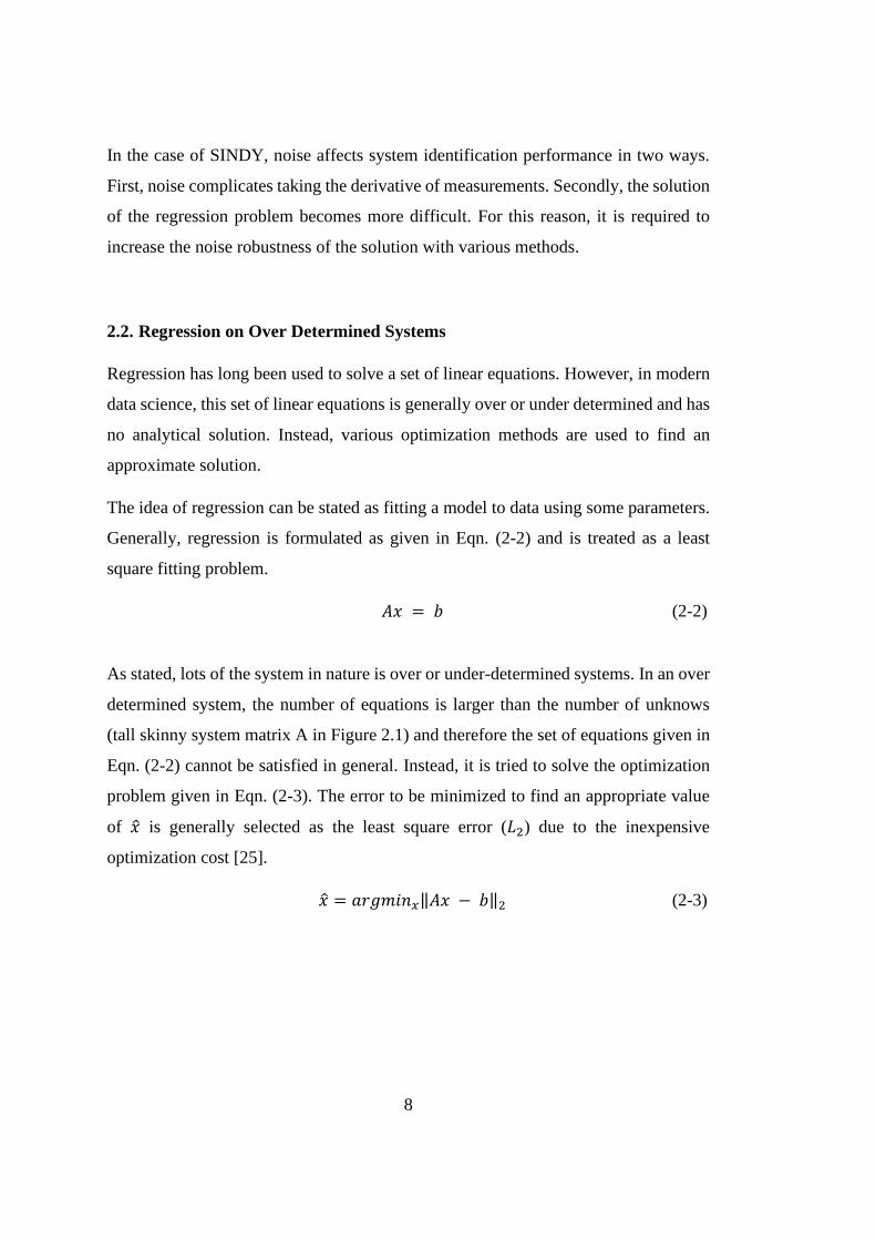
In the case of SINDY, noise affects system identification performance in two ways.
First, noise complicates taking the derivative of measurements. Secondly, the solution
of the regression problem becomes more difficult. For this reason, it is required to
increase the noise robustness of the solution with various methods.
2.2. Regression on Over Determined Systems
Regression has long been used to solve a set of linear equations. However, in modern
data science, this set of linear equations is generally over or under determined and has
no analytical solution. Instead, various optimization methods are used to find an
approximate solution.
The idea of regression can be stated as fitting a model to data using some parameters.
Generally, regression is formulated as given in Eqn. (2-2) and is treated as a least
square fitting problem.
𝐴𝑥 = 𝑏 (2-2)
As stated, lots of the system in nature is over or under-determined systems. In an over
determined system, the number of equations is larger than the number of unknows
(tall skinny system matrix A in Figure 2.1) and therefore the set of equations given in
Eqn. (2-2) cannot be satisfied in general. Instead, it is tried to solve the optimization
problem given in Eqn. (2-3). The error to be minimized to find an appropriate value
of �̂� is generally selected as the least square error (𝐿2) due to the inexpensive
optimization cost [25].
�̂� = 𝑎𝑟𝑔𝑚𝑖𝑛𝑥‖𝐴𝑥 − 𝑏‖2 (2-3)

9
Figure 2.1. The shape of matrices for overdetermined system
In general, solution architecture given in Eqn. (2-3) does not give satisfactory results
without any constraint on the solution of 𝑥. Therefore, optimization formulation is
modified to enforce both minimizing the least square error and satisfying the
constraint on the 𝑥. Parameters 𝜆1 and 𝜆2 given in Eqn. (2-4) are the penalization of
the 𝐿1 and 𝐿2 norms, respectively.
�̂� = 𝑎𝑟𝑔𝑚𝑖𝑛𝑥(‖𝐴𝑥 − 𝑏‖2 + 𝜆1‖𝑥‖1 + 𝜆2‖𝑥‖2) (2-4)
The terms including 𝜆1,2 and 𝐿1,2 norms are called regularization in machine learning
literature. Some form of regularization is required and very important for model
selection, which will be discussed in following section.
2.3. Sparsity Promoting Algorithms
In order to solve overdetermined regression problems, some form of regularization
should be used to promote sparsity in the solution. The commonly used sparsity
promoting methods are 𝐿1 (Lasso), 𝐿2 (Ridge) and Elastic Net regularizations.
In Ridge regression, the penalty term equivalent to square of the magnitude of
coefficients is added to regression equation that is term 𝜆2 in Eqn. (2-4) becomes non-

10
zero and 𝜆1 is zero. On the other hand, in Lasso regression, 𝜆2 in Eqn. (2-4) are set
to zero and 𝜆1 is non-zero. In Elastic Net regression, both 𝜆1 and 𝜆2 are non-zero in
Eqn. (2-4).
Furthermore, “sequential threshold least square algorithm” proposed by [18] is
another powerful sparsity promoting algorithm which is an extension of hard
thresholded regression. Initially coefficients of the unknown dynamical system are
found by ordinary least square (LS) solution without any regularization. Then the
coefficients smaller than some cut-off value is hard thresholded that is forced to be
zero. Next, using the remaining active terms, new ordinary LS solution is obtained for
non-zero indices. This new solution is thresholded again. This procedure is repeated
until all the coefficients are above the threshold value. Finally, the coefficients of the
unknown dynamical system are obtained with promoting sparsity.
The final sparsity promoting algorithm is called Stepwise Sparse Regression (SSR)
algorithm [21] and is inspired by previously mentioned sequential thresholded
regression[18]. In SSR, thresholding approach is modified to remove only one
coefficient per iteration to enforce sparsity. This modification eliminates the need of
searching a threshold parameter and has the best accuracy and rate of convergence
performance among the other applications. However, absence of model selection that
penalizes the number of terms result in solutions that are not sparse enough. Therefore,
it is seen that SSR algorithm may converge to non-sparse collinear basis depending
on the library selection.
In this study, the SSR algorithm will be used to promote sparsity to the solution of
regression equation whereas AIC model selection is included to solve the issues
encountered during SSR implementation.
To sum up, all methods reduce the complexity of regression equation to prevent
overfitting by means of penalizing the coefficients in the solution using different
approaches.
11
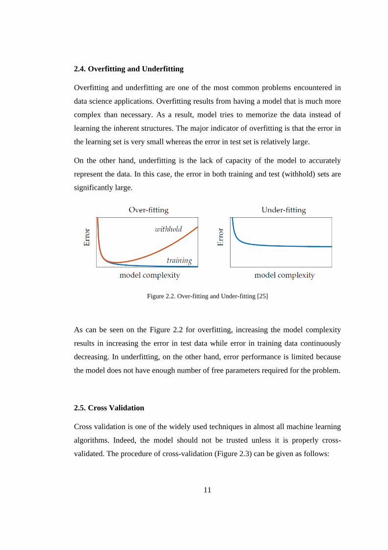
2.4. Overfitting and Underfitting
Overfitting and underfitting are one of the most common problems encountered in
data science applications. Overfitting results from having a model that is much more
complex than necessary. As a result, model tries to memorize the data instead of
learning the inherent structures. The major indicator of overfitting is that the error in
the learning set is very small whereas the error in test set is relatively large.
On the other hand, underfitting is the lack of capacity of the model to accurately
represent the data. In this case, the error in both training and test (withhold) sets are
significantly large.
Figure 2.2. Over-fitting and Under-fitting [25]
As can be seen on the Figure 2.2 for overfitting, increasing the model complexity
results in increasing the error in test data while error in training data continuously
decreasing. In underfitting, on the other hand, error performance is limited because
the model does not have enough number of free parameters required for the problem.
2.5. Cross Validation
Cross validation is one of the widely used techniques in almost all machine learning
algorithms. Indeed, the model should not be trusted unless it is properly cross-
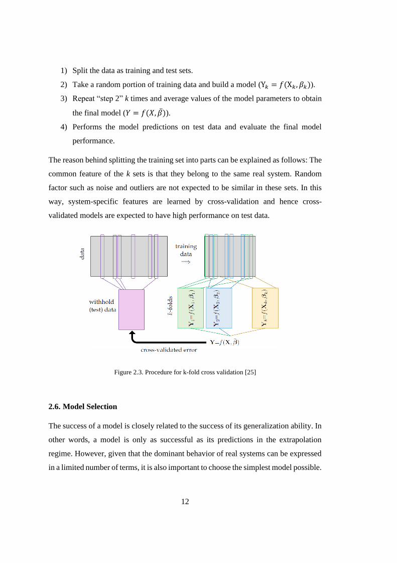
validated. The procedure of cross-validation (Figure 2.3) can be given as follows:
12
1) Split the data as training and test sets.
2) Take a random portion of training data and build a model (Y𝑘 = 𝑓(X𝑘 , 𝛽𝑘)).
3) Repeat “step 2” k times and average values of the model parameters to obtain
the final model (𝑌 = 𝑓(𝑋, �̅�)).
4) Performs the model predictions on test data and evaluate the final model
performance.
The reason behind splitting the training set into parts can be explained as follows: The
common feature of the k sets is that they belong to the same real system. Random
factor such as noise and outliers are not expected to be similar in these sets. In this
way, system-specific features are learned by cross-validation and hence cross-
validated models are expected to have high performance on test data.
Figure 2.3. Procedure for k-fold cross validation [25]
2.6. Model Selection
The success of a model is closely related to the success of its generalization ability. In
other words, a model is only as successful as its predictions in the extrapolation
regime. However, given that the dominant behavior of real systems can be expressed
in a limited number of terms, it is also important to choose the simplest model possible.
13
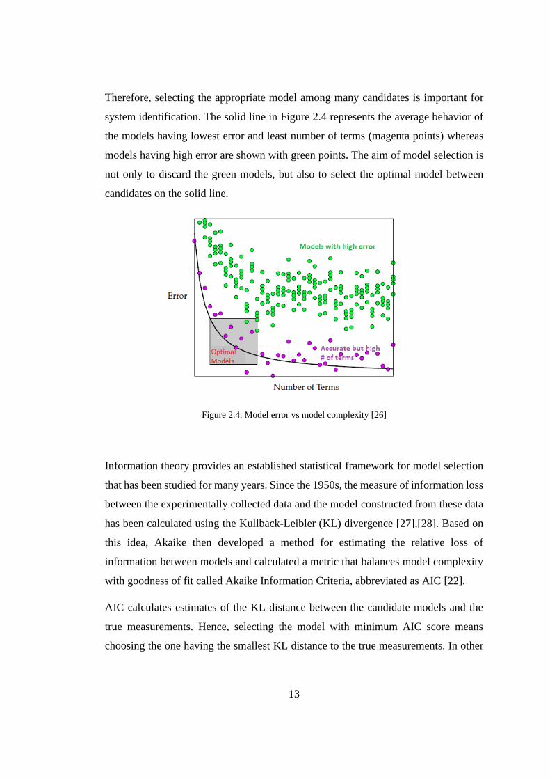
Therefore, selecting the appropriate model among many candidates is important for
system identification. The solid line in Figure 2.4 represents the average behavior of
the models having lowest error and least number of terms (magenta points) whereas
models having high error are shown with green points. The aim of model selection is
not only to discard the green models, but also to select the optimal model between
candidates on the solid line.
Figure 2.4. Model error vs model complexity [26]
Information theory provides an established statistical framework for model selection
that has been studied for many years. Since the 1950s, the measure of information loss
between the experimentally collected data and the model constructed from these data
has been calculated using the Kullback-Leibler (KL) divergence [27],[28]. Based on
this idea, Akaike then developed a method for estimating the relative loss of
information between models and calculated a metric that balances model complexity
with goodness of fit called Akaike Information Criteria, abbreviated as AIC [22].
AIC calculates estimates of the KL distance between the candidate models and the
true measurements. Hence, selecting the model with minimum AIC score means
choosing the one having the smallest KL distance to the true measurements. In other

14
words, AIC is used to compare and select candidate models. The AIC score for each
candidate model j can be calculated using Eqn. (2-5).
𝐴𝐼𝐶𝑗 = 2𝑘 − 2𝑙𝑛(𝐿(𝑥, �̂�)) (2-5)
where k is the number of free parameters which corresponds to model complexity,
𝐿(𝑥, �̂�) = 𝑃(𝑥|𝜇) is the likelihood function of measurements 𝑥 given candidate model
parameters 𝜇 [22].
In general, for finite sample size AIC score formulation requires a correction [29] as
given in Eqn. (2-6);
𝐴𝐼𝐶𝑐 = 𝐴𝐼𝐶 + 2(𝑘 + 1)(𝑘 + 2)/( 𝑚 − 𝑘 − 2) (2-6)
where 𝑚 is the number of observations and 𝐴𝐼𝐶𝑐 is the corrected AIC score.
If residual sum of squares (RSS) is used in likelihood function, AIC formulation
becomes as given in Eqn. (2-7)
𝐴𝐼𝐶 = 𝑚 ∙ 𝑙𝑛(𝑅𝑆𝑆/𝑚) + 2𝑘 (2-7)
where 𝑅𝑆𝑆 = ∑ (𝑦𝑖 − 𝑔(𝑥𝑖; 𝜇))2𝑚𝑖=1 and 𝑔 is the candidate model and 𝑦𝑖 , 𝑥𝑖 are the
observed outcomes and independent variables, respectively.
Note that Eqn. (2-7) penalizes models that have many free parameters and do not
match with the observed outputs by increasing their AIC scores. An example AIC
scores of the candidate models with increasing number of terms is given in Figure 2.5.
As can be seen, if AIC model selection is applied to these candidate models, the model
having 5 number of terms will be selected.
Note that AIC scores are stated as relative to each other. In other words, the minimum
of the AIC score of the candidate models is found first and subtracted from all scores.
Therefore, the minimum AIC score value is always equal to zero and does not always
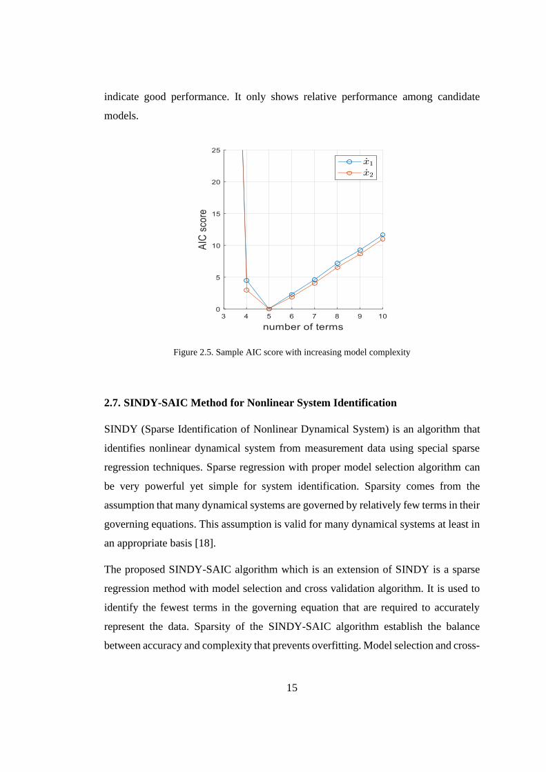
15
indicate good performance. It only shows relative performance among candidate
models.
Figure 2.5. Sample AIC score with increasing model complexity
2.7. SINDY-SAIC Method for Nonlinear System Identification
SINDY (Sparse Identification of Nonlinear Dynamical System) is an algorithm that
identifies nonlinear dynamical system from measurement data using special sparse
regression techniques. Sparse regression with proper model selection algorithm can
be very powerful yet simple for system identification. Sparsity comes from the
assumption that many dynamical systems are governed by relatively few terms in their
governing equations. This assumption is valid for many dynamical systems at least in
an appropriate basis [18].
The proposed SINDY-SAIC algorithm which is an extension of SINDY is a sparse
regression method with model selection and cross validation algorithm. It is used to
identify the fewest terms in the governing equation that are required to accurately
represent the data. Sparsity of the SINDY-SAIC algorithm establish the balance
between accuracy and complexity that prevents overfitting. Model selection and cross-

16
validation allow the selection of the model with the fewest terms and at the same time
having most representation capacity among the many candidate models. Therefore,
SINDY-SAIC is not only a regression method, but it is a set of algorithms that are
used to obtain a system model from measurement data.
In general, many system identification techniques such as neural networks result in
black box models which are difficult to examine and control. On the other hand,
SINDY-SAIC explicitly gives dominant terms in the governing equations.
The general flow of SINDY-SAIC algorithm is given in Figure 2.6.
Figure 2.6. Schematic of SINDY-SAIC algorithm
To find unknown and possibly non-linear system of equations purely from data using
SINDY-SAIC, following algorithm can be used.

17
Step 1. Measure 𝑥𝑖(𝑡𝑗)
𝑥𝑖(𝑡𝑗) is the measurement of the ith state of the system at time j. In other words,
i is the subscript for states of the system ranging from 1 to the number of states
n and j is the subscript for the measurements ranging from 1 to the number of
measurements m. For example, a system can have 1000 measurements and 2
states such as position and velocity.
Step 2. Split measurement data into training and test sets and select number of folds k
for cross validation. Selection of k mainly depends on the time response characteristics
of the interested dynamical system and quality of measurement data. It is not
recommended to select too large k value that will prevent the transient and steady state
behavior to occur.
Step 3. Construct the measurement matrix 𝑋 from training data.
𝑋 = [
𝑥1(𝑡1)
𝑥1(𝑡2)⋮
𝑥1(𝑡𝑚)
𝑥2(𝑡1) ⋯ 𝑥𝑛(𝑡1)
𝑥2(𝑡2) ⋯ 𝑥𝑛(𝑡2)⋮ ⋱ ⋮
𝑥2(𝑡𝑚) ⋯ 𝑥𝑛(𝑡𝑚)
] (2-8)
Step 4. Calculate derivative �̇�𝑖(𝑡𝑗) and construct the matrix �̇�
• �̇�𝑖(𝑡𝑗) is the derivative of measurement data. Derivative is calculated using
proper methods. Note that in case of noisy data, using difference formulas to
calculate derivative generally fails. Therefore, in this study local slope for a
sequence of points is estimated using sliding window approach. In this
approach, a polynomial of given model order is fitted to the noisy data of
selected windows size. Then the polynomial derivative is taken.

18
�̇� = [
�̇�1(𝑡1)
�̇�1(𝑡2)⋮
�̇�1(𝑡𝑚)
�̇�2(𝑡1) ⋯ �̇�𝑛(𝑡1)
�̇�2(𝑡2) ⋯ �̇�𝑛(𝑡2)⋮ ⋱ ⋮
�̇�2(𝑡𝑚) ⋯ �̇�𝑛(𝑡𝑚)
] (2-9)
Step 5. Select the library of candidate functions and construct the matrix Θ
Proper choice of candidate function is crucial for success of SINDY
algorithms. In general, polynomials up to order n and trigonometric functions
are used as library functions. Note that it is better to choose library functions
from a wide range and gradually reduce them. Also, already known terms in
the equation of the dynamical system can be selected as library functions.
𝑋𝑢 = [
𝑥1(𝑡1)
𝑥1(𝑡2)⋮
𝑥1(𝑡𝑚)
𝑥2(𝑡1) ⋯ 𝑥𝑛(𝑡1)
𝑥2(𝑡2) ⋯ 𝑥𝑛(𝑡2)⋮ ⋱ ⋮
𝑥2(𝑡𝑚) ⋯ 𝑥𝑛(𝑡𝑚)
|𝑢] (2-10)
where 𝑋𝑢 is the “augmented state-control matrix” formed by state 𝑋 and control input
𝑢.
Θ(𝑋𝑢) = [
| | | | ⋯ | | | | ⋯
1 𝑋𝑢 𝑋𝑢𝑃2 𝑋𝑢
𝑃3 ⋯ 𝑠𝑖𝑛(𝑋𝑢) 𝑐𝑜𝑠(𝑋𝑢) 𝑠𝑖𝑛(2𝑋𝑢) 𝑐𝑜𝑠(2𝑋𝑢) ⋯| | | | ⋯ | | | | ⋯
] (2-11)
𝑋𝑢𝑃2 =
[ 𝑥1
2(𝑡1)
𝑥12(𝑡2)⋮⋮
𝑥12(𝑡𝑚)
𝑥1(𝑡1)𝑥2(𝑡1) ⋯ 𝑥1(𝑡1)𝑢 𝑥22(𝑡1) 𝑥2(𝑡1)𝑥3(𝑡1) 𝑥2(𝑡1)𝑢 ⋯ 𝑥𝑛
2(𝑡1)
𝑥1(𝑡2)𝑥2(𝑡2) ⋯ 𝑥1(𝑡2)𝑢 𝑥22(𝑡2) 𝑥2(𝑡2)𝑥3(𝑡2) 𝑥2(𝑡2)𝑢 ⋯ 𝑥𝑛(𝑡2)
⋮ ⋮ ⋮ ⋮ ⋮ ⋮ ⋮ ⋮⋮ ⋮ ⋮ ⋮ ⋮ ⋮ ⋮ ⋮
𝑥1(𝑡𝑚)𝑥2(𝑡𝑚) ⋯ 𝑥1(𝑡𝑚)𝑢 𝑥22(𝑡𝑚) 𝑥2(𝑡𝑚)𝑥3(𝑡𝑚) 𝑥2(𝑡𝑚)𝑢 ⋯ 𝑥𝑛(𝑡𝑚)]
(2-12)
Step 6. Solve for coefficient matrix C using Stepwise Sparse Regression (SSR)
technique [21] on training data.
Each column of C contains the sparse coefficient for every row of the
governing equations. Sparsity is promoted during the calculation of C.

19
�̇� = Θ(𝑋𝑢)C (2-13)
𝐶 = [𝑐1 𝑐2 … 𝑐𝑛] (2-14)
Step 7. Perform cross-validation on k folded test data and calculate the error in test
data. Error is defined as residual sum of square (RSS) of the difference between the
true and prediction value in the test data.
Step 8. Using the RSS error and the number of terms in the candidate models, apply
Akaike Information Criteria (AIC) to select the appropriate model among many others
using Eqn. (2-6).
The SINDY-SAIC algorithm provides a suitable environment for model discovery and
selection. The discovered model will be more useful when used in conjunction with a
data-driven control method such as Model Predictive Control. In the next chapter, the
details about MPC will be given.


21
CHAPTER 3
3. MODEL PREDICTIVE CONTROL
MPC is a control strategy that uses a model to predict future plant output and solves
an optimization problem with constraints to select the optimal control action. MPC is
multi variable controller that can handle multi-input multi-output systems and can
handle constraints that prevent the system from undesired consequences [30].
However, MPC requires a powerful, fast processing units and a large amount of
memory because it solves an online optimization problem at each time step. In general,
linear MPC solve the convex quadratic problem, thereby requires less computational
power. On the other hand, nonlinear MPC solves non-convex optimization problem,
thereby requires much more processing power, memory, and time [11]. Considering
the rapid development of computational capacities, it is not difficult to predict that the
use of nonlinear MPC will increase sharply in the near future.
3.1. Working Principle of MPC
MPC is formulated as an open-loop optimization problem. As with all optimization
problems, MPC has a cost function to minimize and constraints to satisfy at each time
step. The basic working principle of MPC is as follows: At current time 𝑡0, future
prediction up to 𝑡0 + 𝐻𝑝 (prediction horizon) time is calculated using the approximate
model of the real system and is called output prediction. Next, the cost function is
calculated using the difference between the set point and the output prediction. By
using a proper optimization routine, the cost function and constraints are tried to be
satisfied and the control input u is calculated. Usually, the control input u is kept
constant after time 𝑡0 + 𝐻𝑚 (control horizon) during the calculation of the output
prediction. Finally, only the first value of the control input is applied to the system and
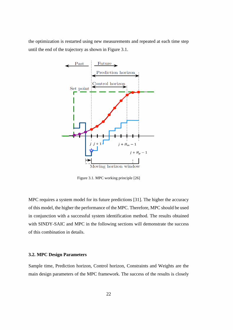
22
the optimization is restarted using new measurements and repeated at each time step
until the end of the trajectory as shown in Figure 3.1.
Figure 3.1. MPC working principle [26]
MPC requires a system model for its future predictions [31]. The higher the accuracy
of this model, the higher the performance of the MPC. Therefore, MPC should be used
in conjunction with a successful system identification method. The results obtained
with SINDY-SAIC and MPC in the following sections will demonstrate the success
of this combination in details.
3.2. MPC Design Parameters
Sample time, Prediction horizon, Control horizon, Constraints and Weights are the
main design parameters of the MPC framework. The success of the results is closely

23
dependent on the appropriate selection of these design parameters. Therefore, in this
section, some recommendations for the selection of these parameters will be given.
3.2.1. Sample Time ( 𝑇𝑠 )
𝑇𝑠 is the rate at which the controller executes the controller algorithm. The large
sample time means that the controller cannot react fast enough to disturbances and
changes in the reference input. On the other hand, in case of very small sample time
controller can react much faster to disturbances and set point changes, but this
introduces computational overloads. To balance the performance and the
computational efforts, a general recommendation is to choose sample time between 5
-10 % of the rise time ( 𝑇𝑟 ) of the open loop response.
0.05 𝑇𝑟 ≤ 𝑇𝑠 ≤ 0.1 𝑇𝑟
However, the designers should determine sampling time according to their
performance expectations, available hardware, and other application specific
requirements.
3.2.2. Prediction Horizon ( 𝐻𝑝 )
The number of predicted future time steps is called prediction horizon and determines
how far the controller predicts into the future. In MPC, the model of the system is used
for future predictions and as it is known, no model is perfect. In addition, unexpected
situations may arise during long trajectories. Therefore, long-term predictions are not
very accurate. Choosing a large prediction horizon does not offer much benefit, but
also increases the computational burden. On the other hand, very small prediction
horizon should not be chosen than the system dynamics allows. The general
recommendation is to choose prediction horizon bigger than the settling time
(𝑇𝑠𝑒𝑡𝑡𝑙𝑖𝑛𝑔 ) of the open loop response.
𝐻𝑝 ≥ 𝑇𝑠𝑒𝑡𝑡𝑙𝑖𝑛𝑔
𝑇𝑠

24
3.2.3. Control Horizon ( 𝐻𝑚 )
The number of steps after which the control remains constant is called the control
horizon. Control horizon determines the number of free variables to be chosen by the
optimizer. So, the smaller the control horizon, the fewer the computations. Too small
control horizon worsens the future predictions. The rule of thumb to choose control
horizon is between 10-20% of the prediction horizon and having 2-3 steps at least.
0.1 𝐻𝑝 ≤ 𝐻𝑚 ≤ 0.2 𝐻𝑝
3.2.4. Constraints
In MPC, constraints on inputs, rate of change of inputs and outputs can be
incorporated. These constraints can be soft and hard constraints. Hard constraints
cannot be violated whereas soft constraints can be violated. Hard constraints generally
come from the physical limits such as maximum allowable deflection of a missile
canard, or the gas pedal limits of a car. On the other hand, soft limits are mostly due
to performance requirements and measures taken to prevent the system from
approaching operating limits of some of the subsystems. Setting hard constraints on
both input and output at the same time should be avoided as these requirements may
conflict and leading to an unfeasible solution for optimization.
3.2.5. Weights
In MPC, multiple goals are present, such as reference tracking and smooth control
input. The importance of these goals relative to each other are specified with weights.
In addition, reference tracking of the outputs can be weighted within itself. For
example, if the reference tracking of the first output is important than the second,
bigger weight should be selected for the first output.

25
3.3. Prediction Formulation and Solution of MPC Problems
Linearized, discrete time state space model of a dynamical system can be given in the
form
𝑥(𝑘 + 1) = 𝐴𝑥(𝑘) + 𝐵𝑢(𝑘)
𝑦(𝑘) = C𝑦𝑥(𝑘)
𝑧(𝑘) = C𝑧𝑥(𝑘)
(3-1)
where x is the state vector, y is the measured outputs, z is the outputs which are to be
controlled and u is the input vector. Generally, y and z are the same that is all
controlled outputs frequently are measured.
The general formulation of the controlled output z is given in Eqn. (3-2)
𝑧(𝑘) = 𝐶𝑧𝑥(𝑘) + 𝐷𝑧𝑢(𝑘) (3-2)
However, 𝐷𝑧 is assumed to be zero in this study for the ease of computation of optimal
𝑢(𝑘). If in real system, 𝐷𝑧 is not equal to zero, this complication can be avoided by
defining a new variable as follows,
�̃�(𝑘) = 𝑧(𝑘) − 𝐷𝑧𝑢(𝑘) (3-3)
3.3.1. Prediction Formulation
The predicted values of the controlled variables �̂�(𝑘 + 𝑖|𝑘) should be calculated using
the estimate of the current state �̂�(𝑘|𝑘), the latest input 𝑢(𝑘 − 1) and the assumed
future input changes ∆�̂�(𝑘 + 𝑖|𝑘).
In case of no disturbances and full state measurements that is �̂�(𝑘|𝑘) = 𝑥(𝑘) = 𝑦(𝑘),
the future prediction of states can be calculated simply by iterating the state space
model as derived in Eqn. (3-4),
26
�̂�(𝑘 + 1|𝑘) = 𝐴𝑥(𝑘) + 𝐵�̂�(𝑘|𝑘)
�̂�(𝑘 + 2|𝑘) = 𝐴�̂�(𝑘 + 1|𝑘) + 𝐵�̂�(𝑘 + 1|𝑘)
= 𝐴2𝑥(𝑘) + 𝐴𝐵�̂�(𝑘|𝑘) + 𝐵�̂�(𝑘 + 1|𝑘)
.
.
�̂�(𝑘 + 𝐻𝑝|𝑘) = 𝐴�̂�(𝑘 + 𝐻𝑝 − 1|𝑘) + 𝐵�̂�(𝑘 + 𝐻𝑝 − 1|𝑘)
= 𝐴𝐻𝑝𝑥(𝑘) + 𝐴𝐻𝑝−1𝐵�̂�(𝑘|𝑘)+. . . +𝐵�̂�(𝑘 + 𝐻𝑝 − 1|𝑘)
(3-4)
For the sake of optimization, it is better to express predictions in terms of ∆�̂�(𝑘 +
𝑖|𝑘) rather than �̂�(𝑘 + 𝑖|𝑘). Note that ∆�̂�(𝑘 + 𝑖|𝑘) = �̂�(𝑘 + 𝑖|𝑘) − �̂�(𝑘 + 𝑖 − 1|𝑘),
then,
�̂�(𝑘|𝑘) = ∆�̂�(𝑘|𝑘) + 𝑢(𝑘 − 1)
�̂�(𝑘 + 1|𝑘) = ∆�̂�(𝑘 + 1|𝑘) + ∆�̂�(𝑘|𝑘) + 𝑢(𝑘 − 1)
.
.
�̂�(𝑘 + 𝐻𝑚 − 1|𝑘) = ∆�̂�(𝑘 + 𝐻𝑚 − 1|𝑘)+. . . +∆�̂�(𝑘|𝑘) + 𝑢(𝑘 − 1)
(3-5)
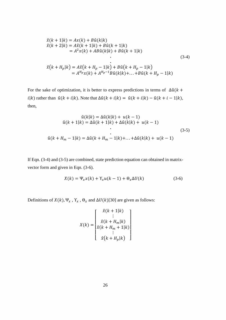
If Eqn. (3-4) and (3-5) are combined, state prediction equation can obtained in matrix-
vector form and given in Eqn. (3-6).
𝑋(𝑘) = Ψ𝑥𝑥(𝑘) + Υ𝑥𝑢(𝑘 − 1) + Θ𝑥∆𝑈(𝑘) (3-6)
Definitions of 𝑋(𝑘),Ψ𝑥 , Υ𝑥 , Θ𝑥 and ∆𝑈(𝑘)[30] are given as follows:
𝑋(𝑘) =
[
�̂�(𝑘 + 1|𝑘)⋮
�̂�(𝑘 + 𝐻𝑚|𝑘)
�̂�(𝑘 + 𝐻𝑚 + 1|𝑘)⋮
�̂�(𝑘 + 𝐻𝑝|𝑘) ]
27
Ψ𝑥 =
[
𝐴⋮
𝐴𝐻𝑚
𝐴𝐻𝑚+1
⋮𝐴𝐻𝑝 ]
, Υ𝑥 =
[
𝐵⋮
∑ 𝐴𝑖𝐵𝐻𝑚−1
𝑖=0
∑ 𝐴𝑖𝐵𝐻𝑚
𝑖=0
⋮
∑ 𝐴𝑖𝐵𝐻𝑝−1
𝑖=0 ]
Θ𝑥 =
[
𝐵 ⋯ 0𝐴𝐵 + 𝐵 ⋯ 0
⋮ ⋱ ⋮
∑ 𝐴𝑖𝐵𝐻𝑚−1
𝑖=0⋯ 𝐵
∑ 𝐴𝑖𝐵𝐻𝑚
𝑖=0⋯ 𝐴𝐵 + 𝐵
⋮ ⋮ ⋮
∑ 𝐴𝑖𝐵𝐻𝑝−1
𝑖=0⋯ ∑ 𝐴𝑖𝐵
𝐻𝑝−𝐻𝑚
𝑖=0 ]
𝑎𝑛𝑑 ∆𝑈(𝑘) = [∆�̂�(𝑘|𝑘)
⋮∆�̂�(𝑘 + 𝐻𝑚 − 1|𝑘)
]
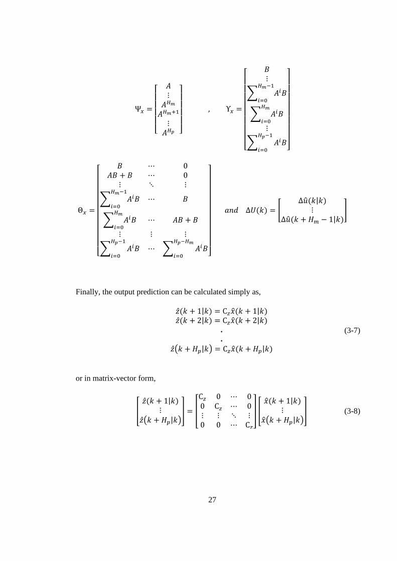
Finally, the output prediction can be calculated simply as,
�̂�(𝑘 + 1|𝑘) = C𝑧�̂�(𝑘 + 1|𝑘)
�̂�(𝑘 + 2|𝑘) = C𝑧�̂�(𝑘 + 2|𝑘)
.
.
�̂�(𝑘 + 𝐻𝑝|𝑘) = C𝑧�̂�(𝑘 + 𝐻𝑝|𝑘)
(3-7)
or in matrix-vector form,
[
�̂�(𝑘 + 1|𝑘)⋮
�̂�(𝑘 + 𝐻𝑝|𝑘)] = [
C𝑧 0 ⋯ 00 C𝑧 ⋯ 0⋮ ⋮ ⋱ ⋮0 0 ⋯ C𝑧
] [
�̂�(𝑘 + 1|𝑘)⋮
�̂�(𝑘 + 𝐻𝑝|𝑘)] (3-8)

28
3.3.2. Solution of MPC Problem
𝑍(𝑘) = [
�̂�(𝑘 + 𝐻𝑤|𝑘)⋮
�̂�(𝑘 + 𝐻𝑝|𝑘)] , 𝑇(𝑘) = [
�̂�(𝑘 + 𝐻𝑤|𝑘)⋮
�̂�(𝑘 + 𝐻𝑝|𝑘)], ∆𝑈(𝑘) = [
∆�̂�(𝑘|𝑘)⋮
∆�̂�(𝑘 + 𝐻𝑚 − 1|𝑘)]
𝑍(𝑘), 𝑇(𝑘), ∆𝑈(𝑘) are the outputs, reference (Target trajectory) and change in the
control inputs respectively. Note that if the start index (𝐻𝑤) is selected greater than
unity, it means that the deviations of 𝑧 from 𝑟 are not penalized immediately. If Eqn.
(3-6) and (3-8) are combined with the 𝑍(𝑘), 𝑇(𝑘), ∆𝑈(𝑘) definitions, the following
output prediction equation is obtained,
𝑍(𝑘) = Ψ𝑥(𝑘) + Υ𝑢(𝑘 − 1) + Θ∆𝑈(𝑘) (3-9)
where
Ψ = [
C𝑧 0 ⋯ 00 C𝑧 ⋯ 0⋮ ⋮ ⋱ ⋮0 0 ⋯ C𝑧
]Ψ𝑥 , Υ = [
C𝑧 0 ⋯ 00 C𝑧 ⋯ 0⋮ ⋮ ⋱ ⋮0 0 ⋯ C𝑧
] Υ𝑥
Θ = [
C𝑧 0 ⋯ 00 C𝑧 ⋯ 0⋮ ⋮ ⋱ ⋮0 0 ⋯ C𝑧
]Θ𝑥
The cost function that should be minimized is given as [30],
𝐽(𝑘) = ∑ ‖�̂�(𝑘 + 𝑖|𝑘) − �̂�(𝑘 + 𝑖|𝑘)‖𝑄(𝑖)2
𝐻𝑝
𝑖=𝐻𝑤
+ ∑ ‖∆�̂�(𝑘 + 𝑖|𝑘)‖𝑅(𝑖)2
𝐻𝑚−1
𝑖=0
(3-10)
Or in more compact form,

29
𝐽(𝑘) = ‖𝑍(𝑘) − 𝑇(𝑘)‖𝑄2 + ‖∆𝑈(𝑘)‖𝑅
2 (3-11)
The tracking error Ε, that is the difference between Target trajectory and the “free
response” of the system is
Ε(𝑘) = 𝑇(𝑘) − Ψ𝑥(𝑘) − Υ𝑢(𝑘 − 1) (3-12)
Free response of the system is the output of the system that changes in the input is
zero (∆𝑈(𝑘) = 0).
Using Eqns. (3-11) and (3-12),
𝐽(𝑘) = ‖Θ∆𝑈(𝑘) − Ε(𝑘)‖𝑄2 + ‖∆𝑈(𝑘)‖𝑅
2
= [∆𝑈(𝑘)𝑇Θ𝑇 − Ε(𝑘)𝑇]𝑄[Θ∆𝑈(𝑘) − Ε(𝑘)]+ ∆𝑈(𝑘)𝑇𝑅∆𝑈(𝑘)
= Ε(𝑘)𝑇𝑄Ε(𝑘) − 2∆𝑈(𝑘)𝑇Θ𝑇𝑄Ε(𝑘) + ∆𝑈(𝑘)𝑇[Θ𝑇𝑄Θ + 𝑅] ∆𝑈(𝑘)
(3-13)
Let’s define 𝐺 = 2Θ𝑇𝑄Ε(𝑘) and 𝐻 = Θ𝑇𝑄Θ + 𝑅), then cost equation becomes,
𝐽(𝑘) = 𝑐𝑜𝑛𝑠𝑡 − ∆𝑈(𝑘)𝑇𝐺 + ∆𝑈(𝑘)𝑇𝐻∆𝑈(𝑘) (3-14)
As seen 𝐺 and 𝐻 does not depends on ∆𝑈(𝑘). To find the optimal value of ∆𝑈(𝑘), the
gradient of 𝐽(𝑘) with respect to ∆𝑈(𝑘) should be calculated and set to zero.
∇∆𝑈(𝑘)𝐽 = −𝐺 + 2𝐻∆𝑈(𝑘) → 0
∆𝑈(𝑘)𝑜𝑝𝑡 =
1
2𝐻−𝟏𝐺 (3-15)
As stated, in MPC only the first part of the solution (Eqn. (3-15)) should be used
because of the receding horizon concept. Note that this ensures the closed loop
behavior of MPC.
30
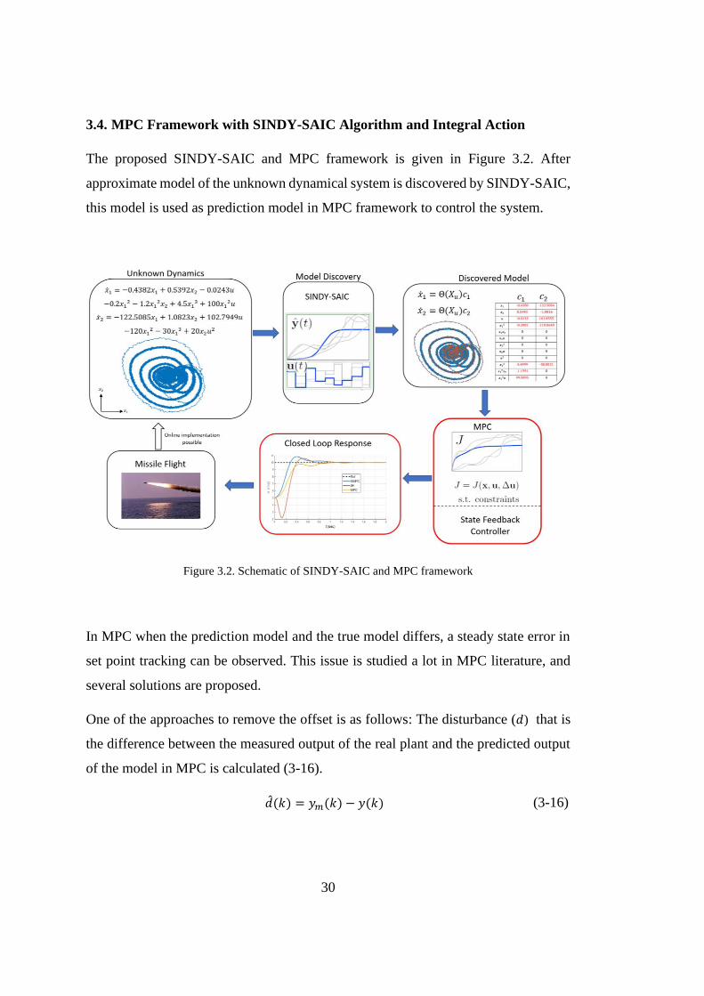
3.4. MPC Framework with SINDY-SAIC Algorithm and Integral Action
The proposed SINDY-SAIC and MPC framework is given in Figure 3.2. After
approximate model of the unknown dynamical system is discovered by SINDY-SAIC,
this model is used as prediction model in MPC framework to control the system.
Figure 3.2. Schematic of SINDY-SAIC and MPC framework
In MPC when the prediction model and the true model differs, a steady state error in
set point tracking can be observed. This issue is studied a lot in MPC literature, and
several solutions are proposed.
One of the approaches to remove the offset is as follows: The disturbance (𝑑) that is
the difference between the measured output of the real plant and the predicted output
of the model in MPC is calculated (3-16).
�̂�(𝑘) = 𝑦𝑚(𝑘) − 𝑦(𝑘) (3-16)
31
The steady state error is removed from the system by shifting the prediction output as
given in Eqn. (3-17). The corrected prediction output (𝑦∗) is fed to the PID controller
to remove the offset from tracking. The assumption that disturbance stays constant is
not valid for some cases, therefore, in this method the offset free tracking cannot be
obtained at all conditions. The details of the implementation can be found in [32].
𝑦∗(𝑘 + 𝑖) = 𝑦(𝑘 + 𝑖) + �̂�(𝑘) (3-17)
Another approach is to include the tracking error into the states of the system by
augmentation [33]. However, this is valid only for linear prediction models and
increases the system order that affects the MPC computation time.
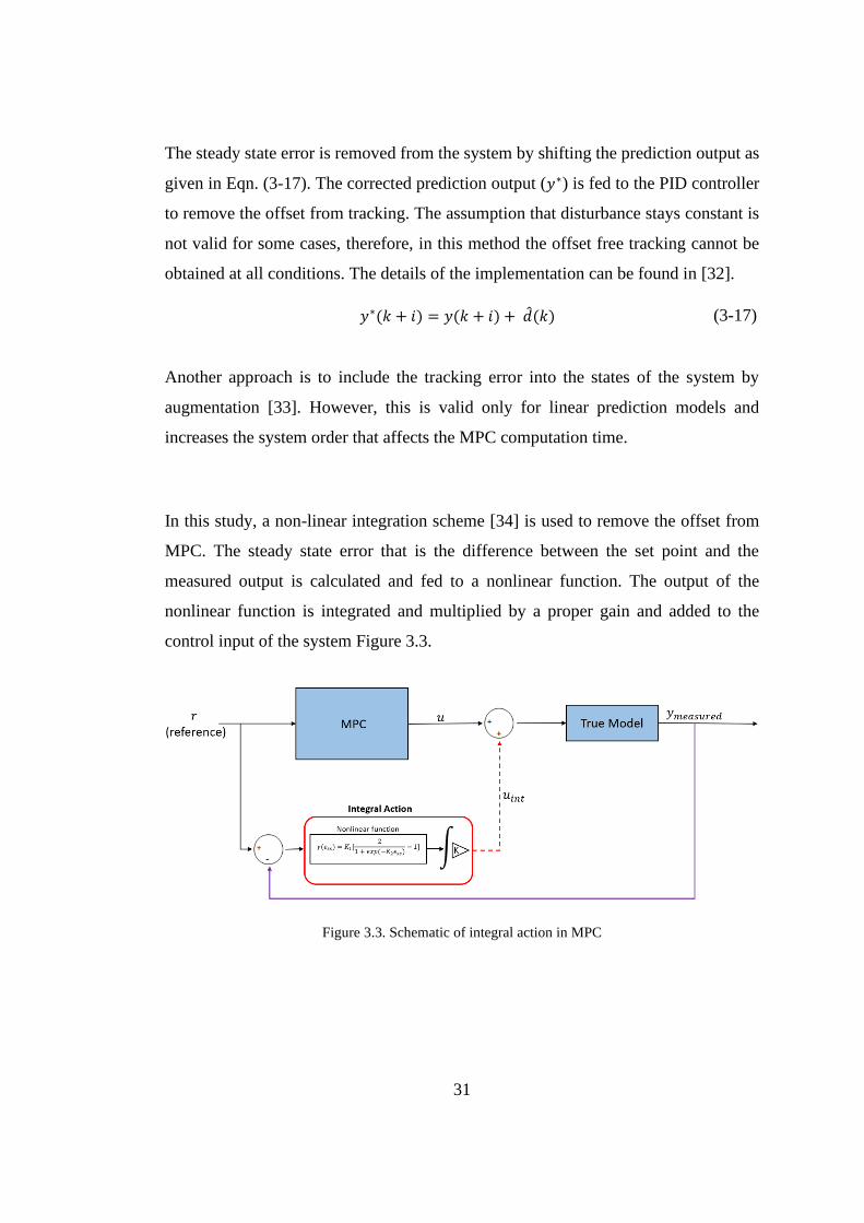
In this study, a non-linear integration scheme [34] is used to remove the offset from
MPC. The steady state error that is the difference between the set point and the
measured output is calculated and fed to a nonlinear function. The output of the
nonlinear function is integrated and multiplied by a proper gain and added to the
control input of the system Figure 3.3.
Figure 3.3. Schematic of integral action in MPC
32
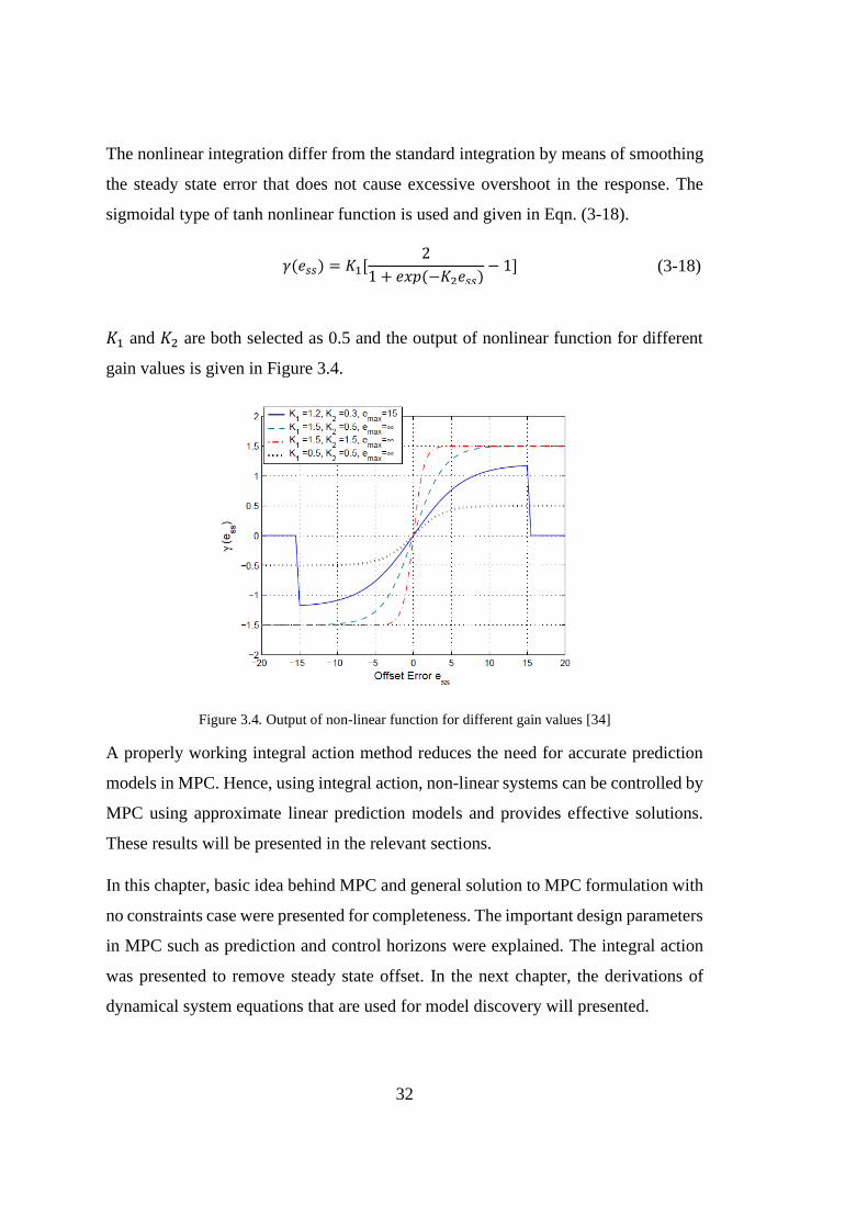
The nonlinear integration differ from the standard integration by means of smoothing
the steady state error that does not cause excessive overshoot in the response. The
sigmoidal type of tanh nonlinear function is used and given in Eqn. (3-18).
𝛾(𝑒𝑠𝑠) = 𝐾1[
2
1 + 𝑒𝑥𝑝(−𝐾2𝑒𝑠𝑠)− 1] (3-18)
𝐾1 and 𝐾2 are both selected as 0.5 and the output of nonlinear function for different
gain values is given in Figure 3.4.
Figure 3.4. Output of non-linear function for different gain values [34]
A properly working integral action method reduces the need for accurate prediction
models in MPC. Hence, using integral action, non-linear systems can be controlled by
MPC using approximate linear prediction models and provides effective solutions.
These results will be presented in the relevant sections.
In this chapter, basic idea behind MPC and general solution to MPC formulation with
no constraints case were presented for completeness. The important design parameters
in MPC such as prediction and control horizons were explained. The integral action
was presented to remove steady state offset. In the next chapter, the derivations of
dynamical system equations that are used for model discovery will presented.
33
CHAPTER 4
4. MISSILE DYNAMIC MODEL AND STATE FEEDBACK CONTROL
In this chapter missile dynamic model that will be discovered using SINDY-SAIC will
be derived using 6 DOF motion equations. Then, the general architecture of state
feedback control used for comparison with MPC will be given.
4.1. Longitudinal Missile Dynamics
6 DOF motion equations [35] are given in Eqn. (4-1) through Eqn. (4-6).
𝐹𝑋 = 𝑚(�̇� + 𝑞𝑤 − 𝑟𝑣 + 𝑔𝑠𝑖𝑛(𝜃)) (4-1)
𝐹𝑌 = 𝑚(�̇� + 𝑟𝑢 − 𝑝𝑤 − 𝑔𝑐𝑜𝑠(𝜃) sin(𝜙)) (4-2)
𝐹𝑧 = 𝑚(�̇� + 𝑝𝑣 − 𝑞𝑢 − 𝑔𝑐𝑜𝑠(𝜃) cos(𝜙)) (4-3)
𝑀𝐿 = 𝐼𝑥𝑥�̇� − 𝐼𝑦𝑧(𝑞2 − 𝑟2) − 𝐼𝑧𝑥(�̇� + 𝑝𝑞) − 𝐼𝑥𝑦(�̇� − 𝑟𝑝)
− (𝐼𝑦𝑦 − 𝐼𝑧𝑧)𝑞𝑟 (4-4)
𝑀𝑀 = 𝐼𝑦𝑦�̇� − 𝐼𝑧𝑥(𝑟2 − 𝑝2) − 𝐼𝑥𝑦(�̇� + 𝑞𝑟) − 𝐼𝑦𝑧(�̇� − 𝑝𝑞)
− (𝐼𝑧𝑧 − 𝐼𝑥𝑥)𝑟𝑝 (4-5)
𝑀𝑁 = 𝐼𝑧𝑧�̇� − 𝐼𝑥𝑦(𝑝2 − 𝑞2) − 𝐼𝑦𝑧(�̇� + 𝑟𝑝) − 𝐼𝑧𝑥(�̇� − 𝑞𝑟)
− (𝐼𝑥𝑥 − 𝐼𝑦𝑦)𝑝𝑞 (4-6)
In this study, only the longitudinal dynamics will be discovered using SINDY-SAIC.
Hence, Eqns. (4-3) and (4-5) are the ones defining the longitudinal motion of the
missile.

34
For rotationally symmetric missiles, cross product of inertia terms is generally
neglected for simplicity that is 𝐼𝑧𝑥 = 𝐼𝑥𝑦 = 𝐼𝑦𝑧 = 0. In addition, roll rate of the missile
is usually controlled by roll autopilot and can be assumed to zero (𝑝 = 0). Hence,
Eqns. (4-3) and (4-5) becomes,
𝐹𝑧 = 𝑚(�̇� − 𝑞𝑢 − 𝑔𝑐𝑜𝑠(𝜃) cos(𝜙)) (4-7)
𝑀𝑀 = 𝐼𝑦𝑦�̇� (4-8)
where 𝑚 is the mass of the missile, 𝑢 and 𝑤 are the body frame velocities in 𝑥 and 𝑧
directions respectively, 𝜙 and 𝜃 are the roll and pitch angles, 𝑞 is the pitch rate, 𝑔 is
the gravitational acceleration, 𝐼𝑦𝑦 is the moment of inertia in longitudinal plane, 𝐹𝑧
and 𝑀𝑀 are the aerodynamic force and moment in longitudinal plane.
During the longitudinal autopilot design, the gravitational acceleration acting on the
missile generally considered as a disturbance, therefore 𝑔 is assumed to be zero.
Hence, simplified longitudinal equations of missile becomes,
𝐹𝑧 = 𝑚(�̇� − 𝑞𝑢) (4-9)
𝑀𝑀 = 𝐼𝑦𝑦�̇� (4-10)
Note that only the terms belonging to longitudinal dynamics exist in Eqns. (4-9) and
(4-10). All the dependence on roll and yaw dynamics are eliminated.
The states that are measured in this study is determined as 𝛼 and 𝑞. Hence, conversion
from 𝑤 to 𝛼 is required. This accomplished by using small angle assumption. Angle
of attack (𝛼) smaller than 15 degrees can be approximated using Eqn. (4-11).
𝛼 = tan−1 (𝑤
𝑢) ≅
𝑤
𝑢 (4-11)

35
The derivative of Eqn. (4-11) under the assumption of constant 𝑢 velocity gives,
�̇� =
�̇�
𝑢 (4-12)
Therefore, the equations of motion in longitudinal plane become,
�̇� =
𝐹𝑧
𝑚𝑢+ 𝑞 (4-13)
�̇� =
𝑀𝑀
𝐼𝑦𝑦 (4-14)
Strong nonlinearity comes from the force and moment terms in Eqns. (4-13) and
(4-14). In this study, 𝐹𝑧 and 𝑀𝑀 are expressed as follows,
𝐹𝑧 = 𝑄𝐴 (𝐶𝑧𝛼 ∙ 𝛼 + 𝐶𝑧𝛿𝑒
∙ 𝛿𝑒 + 𝐶𝑧𝑞 ∙ 𝑞𝑑
2𝑉+ 𝐶𝑧𝛼2
∙ 𝛼2
+ 𝐶𝑧𝑞𝛼2∙ 𝑞𝛼2 + 𝐶𝑧𝛼3
∙ 𝛼3 + 𝐶𝑧𝛼2𝛿𝑒∙ 𝛼2𝛿𝑒)
(4-15)
𝑀𝑀 = 𝑄𝐴𝑙𝑟𝑒𝑓 (𝐶𝑚𝛼 ∙ 𝛼 + 𝐶𝑚𝛿𝑒
∙ 𝛿𝑒 + 𝐶𝑚𝑞 ∙ 𝑞𝑑
2𝑉
+ 𝐶𝑚𝛼2∙ 𝛼2 + 𝐶𝑚𝛼3
∙ 𝛼3 + 𝐶𝑚𝑞𝛿𝑒2∙ 𝑞𝛿𝑒
2)
(4-16)
Note that the type of nonlinearities in 𝐹𝑧 and 𝑀𝑀 can change depending on the
aerodynamic characteristics of the missile.
It is better to use some definition for the clarity of the results. The definitions are given
in Table 4.1.
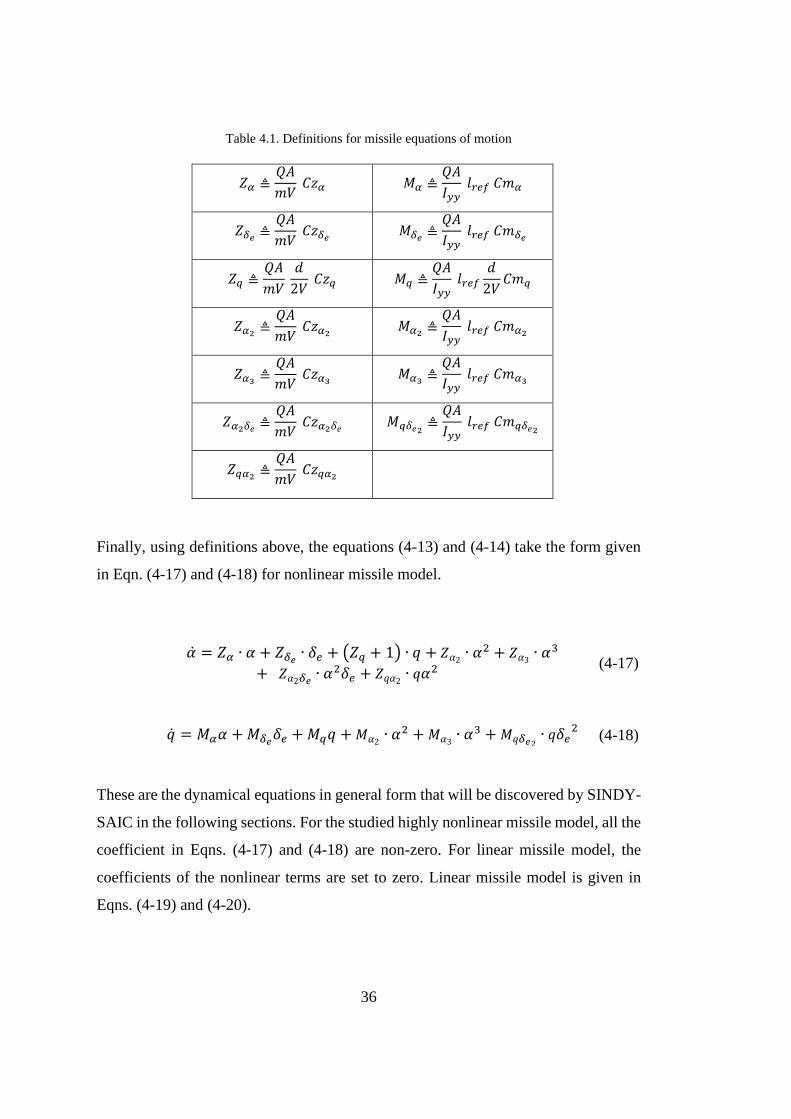
36
Table 4.1. Definitions for missile equations of motion
𝑍𝛼 ≜𝑄𝐴
𝑚𝑉 𝐶𝑧𝛼 𝑀𝛼 ≜
𝑄𝐴
𝐼𝑦𝑦 𝑙𝑟𝑒𝑓 𝐶𝑚𝛼
𝑍𝛿𝑒≜
𝑄𝐴
𝑚𝑉 𝐶𝑧𝛿𝑒
𝑀𝛿𝑒≜
𝑄𝐴
𝐼𝑦𝑦 𝑙𝑟𝑒𝑓 𝐶𝑚𝛿𝑒
𝑍𝑞 ≜𝑄𝐴
𝑚𝑉 𝑑
2𝑉 𝐶𝑧𝑞 𝑀𝑞 ≜
𝑄𝐴
𝐼𝑦𝑦 𝑙𝑟𝑒𝑓
𝑑
2𝑉𝐶𝑚𝑞
𝑍𝛼2≜
𝑄𝐴
𝑚𝑉 𝐶𝑧𝛼2
𝑀𝛼2≜
𝑄𝐴
𝐼𝑦𝑦 𝑙𝑟𝑒𝑓 𝐶𝑚𝛼2
𝑍𝛼3≜
𝑄𝐴
𝑚𝑉 𝐶𝑧𝛼3
𝑀𝛼3≜
𝑄𝐴
𝐼𝑦𝑦 𝑙𝑟𝑒𝑓 𝐶𝑚𝛼3
𝑍𝛼2𝛿𝑒≜
𝑄𝐴
𝑚𝑉 𝐶𝑧𝛼2𝛿𝑒
𝑀𝑞𝛿𝑒2≜
𝑄𝐴
𝐼𝑦𝑦 𝑙𝑟𝑒𝑓 𝐶𝑚𝑞𝛿𝑒2
𝑍𝑞𝛼2≜
𝑄𝐴
𝑚𝑉 𝐶𝑧𝑞𝛼2
Finally, using definitions above, the equations (4-13) and (4-14) take the form given
in Eqn. (4-17) and (4-18) for nonlinear missile model.
�̇� = 𝑍𝛼 ∙ 𝛼 + 𝑍𝛿𝑒
∙ 𝛿𝑒 + (𝑍𝑞 + 1) ∙ 𝑞 + 𝑍𝛼2∙ 𝛼2 + 𝑍𝛼3
∙ 𝛼3
+ 𝑍𝛼2𝛿𝑒∙ 𝛼2𝛿𝑒 + 𝑍𝑞𝛼2
∙ 𝑞𝛼2 (4-17)
�̇� = 𝑀𝛼𝛼 + 𝑀𝛿𝑒𝛿𝑒 + 𝑀𝑞𝑞 + 𝑀𝛼2
∙ 𝛼2 + 𝑀𝛼3∙ 𝛼3 + 𝑀𝑞𝛿𝑒2
∙ 𝑞𝛿𝑒2 (4-18)
These are the dynamical equations in general form that will be discovered by SINDY-
SAIC in the following sections. For the studied highly nonlinear missile model, all the
coefficient in Eqns. (4-17) and (4-18) are non-zero. For linear missile model, the
coefficients of the nonlinear terms are set to zero. Linear missile model is given in
Eqns. (4-19) and (4-20).

37
�̇� = 𝑍𝛼 ∙ 𝛼 + 𝑍𝛿𝑒∙ 𝛿𝑒 + (𝑍𝑞 + 1) ∙ 𝑞 (4-19)
�̇� = 𝑀𝛼𝛼 + 𝑀𝛿𝑒𝛿𝑒 + 𝑀𝑞𝑞 (4-20)
4.2. State Feedback Control
The state space formulation of linear or linearized system (for non-linear missile
model) is given by Eqns. (4-21) and (4-22). Here the states are 𝑥 = [𝛼, 𝑞]𝑇 and the
output to be controlled is angle of attack, 𝛼.
𝑨 = [𝑍𝛼 (𝑍𝑞 + 1)
𝑀𝛼 𝑀𝑞] , 𝑩 = [
𝑍𝛿𝑒
𝑀𝛿𝑒
] (4-21)
𝑪 = [1 0], 𝐷 = [ 0] (4-22)
The plant A has no integrator and therefore an integrator will be added in the
feedforward path. The schematic of the state feedback controller is given in Figure
4.1.
Figure 4.1. State Feedback Controller Structure [36]
From Figure 4.1, the following set of equations can be obtained [36] ,

38
�̇� = 𝑨𝒙 + 𝑩𝑢
𝑦 = 𝑪𝒙
𝑢 = −𝑲𝒙 + 𝑘𝐼𝜉
�̇� = 𝑟 − 𝑦 = 𝑟 − 𝑪𝑥
(4-23)
where 𝑢 is the control input, 𝑦 =output of the system, 𝜉 is the output of the integrator
(augmented state variable) and 𝑟 is the reference signal. If the n dimensional state 𝑥
and the integrator output 𝜉 are augmented to form a new state space model,
Eqns.(4-23) can be expressed in the form,
[ �̇��̇� ] = [
𝑨 𝟎−𝑪 0
] [ 𝒙𝜉 ] + [
𝑩0 ] 𝑢(𝑡) + [
𝟎1 ] 𝑟(𝑡) (4-24)
Note that at steady state 𝜉(t)̇ = 0 and y(∞) = 𝑟.
[ �̇�(∞)
�̇�(∞) ] = [
𝑨 𝟎−𝑪 0
] [ 𝒙(∞)𝜉(∞)
] + [ 𝑩0 ] 𝑢(∞) + [
𝟎1 ] 𝑟(∞) (4-25)
Notice that 𝑟(𝑡) is a step input and hence, 𝑟(∞) = 𝑟(𝑡) = 𝑟.
Subtracting Eqn. (4-25) from (4-24) yields,
[ �̇�𝒆(𝑡)
�̇�𝑒(𝑡) ] = [
𝑨 𝟎−𝑪 0
] [ 𝒙𝒆(𝑡)𝜉𝑒(𝑡)
] + [ 𝑩0 ] 𝑢𝑒(𝑡) (4-26)
where 𝒙𝒆(𝒕) = 𝒙(𝒕) − 𝒙(∞) and same definitions are valid for 𝜉e(t) and 𝑢e(𝑡).
𝑢e(𝑡) = −𝑲𝒙𝐞(𝑡) + 𝑘𝐼𝜉e(t).
In more compact form, Eqn. (4-26) can be given as [36],
�̇� = �̂�𝒆 + �̂�𝑢e (4-27)

39
where
�̂� = [𝑨 𝟎−𝑪 0
] , �̂� = [ 𝑩0 ] , 𝒆 = [
𝒙𝒆
𝜉𝑒 ] , 𝑢e = −�̂�𝑒 (4-28)
�̂� = [𝑲 , −𝑘𝐼]
The error equation of states can be obtained by substituting 𝑢e = −�̂�𝑒 into Eqn.
(4-27).
�̇� = (�̂� − �̂��̂�)𝒆 (4-29)
The desired closed loop poles of the �̂� − �̂��̂� matrix is specified during the design of
the State Feedback (SF) controller in this study. 𝑲 𝑎𝑛𝑑 𝑘𝐼 are determined by means
of pole placement technique.
Note that if the matrix [𝑨 𝑩
−𝑪 0] has rank (n+1), then the system defined by Eqn.
(4-29) is completely controllable [36].
In this section, nonlinear and linear equations of longitudinal missile dynamics were
derived using 6 DOF motion equations. The brief information about state feedback
control were given for completeness.
In the next section, numerical results about SINDY-SAIC algorithm will be presented
as prediction comparison. Then, the comparison of the control methods (MPC, NMPC
and SF) will be given.


41
CHAPTER 5
5. NUMERICAL RESULTS
In this chapter, the results obtained from SINDY-SAIC algorithm will be presented in
Prediction Comparison section. Then, the control performance results of the MPC,
NMPC and SF controllers will be presented using discovered linear and nonlinear
models.
5.1. Prediction Comparison
The prediction performance of SINDY algorithm for the interested dynamical system
is presented in this section.
The dynamical systems whose prediction performances are presented is as follows,
1. Longitudinal Linear Missile Dynamics
2. Longitudinal Highly non-linear Missile Dynamics
5.1.1. Linear Missile Dynamics - Longitudinal
The continuous formulation of linear longitudinal missile dynamic derived earlier is
given in Eqn. (5-1)
�̇� = 𝑍𝛼𝛼 + 𝑍𝛿𝑒
𝛿𝑒 + (𝑍𝑞 + 1)𝑞
�̇� = 𝑀𝛼𝛼 + 𝑀𝛿𝑒𝛿𝑒 + 𝑀𝑞𝑞
(5-1)
where
𝑍𝛼 = −0.4382 𝑍𝛿𝑒= −0.0243 𝑍𝑞 = −0.4608
𝑀𝛼 = −122.5085 𝑀𝛿𝑒= 102.7949 𝑀𝑞 = −1.0823
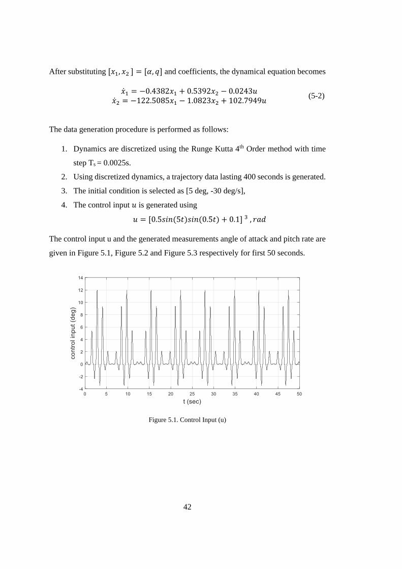
42
After substituting [𝑥1, 𝑥2 ] = [𝛼, 𝑞] and coefficients, the dynamical equation becomes
�̇�1 = −0.4382𝑥1 + 0.5392𝑥2 − 0.0243𝑢
�̇�2 = −122.5085𝑥1 − 1.0823𝑥2 + 102.7949𝑢 (5-2)
The data generation procedure is performed as follows:
1. Dynamics are discretized using the Runge Kutta 4th Order method with time
step Ts = 0.0025s.
2. Using discretized dynamics, a trajectory data lasting 400 seconds is generated.
3. The initial condition is selected as [5 deg, -30 deg/s],
4. The control input 𝑢 is generated using
𝑢 = [0.5𝑠𝑖𝑛(5𝑡)𝑠𝑖𝑛(0.5𝑡) + 0.1] 3 , 𝑟𝑎𝑑
The control input u and the generated measurements angle of attack and pitch rate are
given in Figure 5.1, Figure 5.2 and Figure 5.3 respectively for first 50 seconds.
Figure 5.1. Control Input (u)
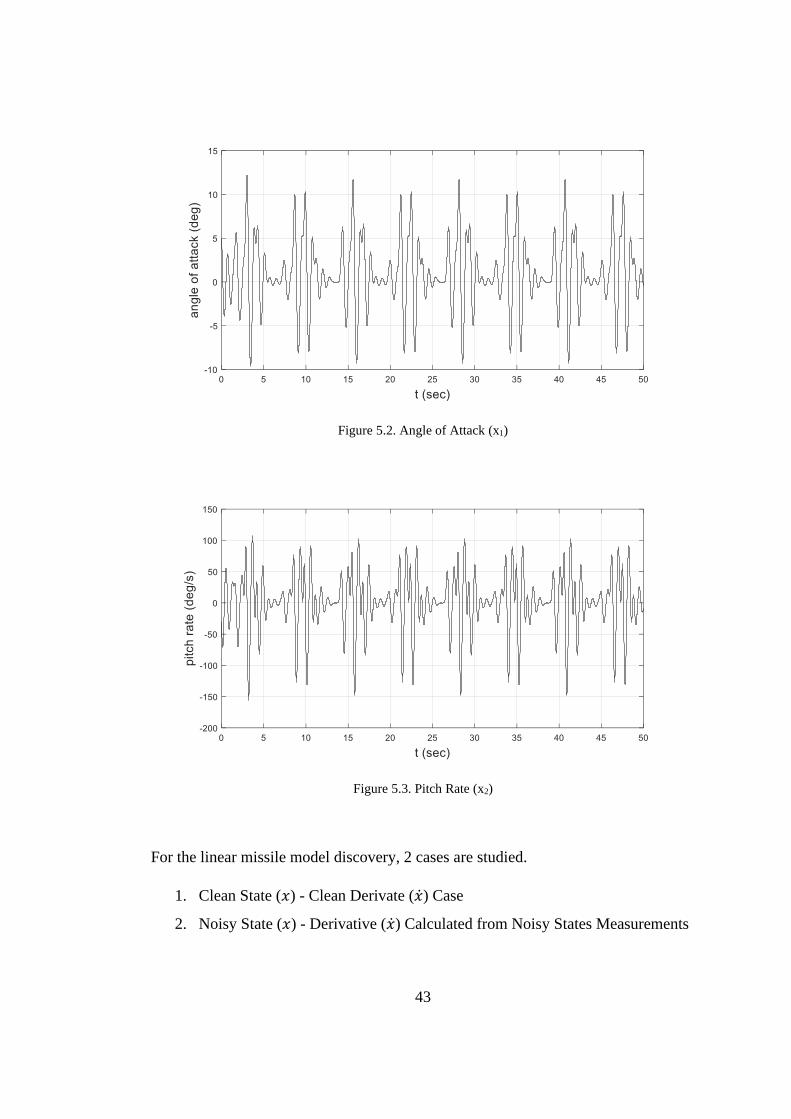
43
Figure 5.2. Angle of Attack (x1)
Figure 5.3. Pitch Rate (x2)
For the linear missile model discovery, 2 cases are studied.
1. Clean State (𝑥) - Clean Derivate (�̇�) Case
2. Noisy State (𝑥) - Derivative (�̇�) Calculated from Noisy States Measurements

44
5.1.1.1. Clean State (𝑥) - Clean Derivative (𝑑𝑥) Case
In this case, it is assumed that states are measured without noise and derivatives are
measured directly or calculated from clean state measurements perfectly.
Polynomial orders up to 2 is used to construct the library functions. Number of terms
in the discovered model is restricted between 1 to 7. All the models that SINDY
generated are given in Table 5.1. According to the AIC scores of these models, the
model with the minimum AIC score is selected. As can be seen in Figure 5.4, the
minimum AIC scores is obtained for the models with 3 number of terms both for �̇�1
and �̇�2 equations.
Table 5.1. Candidate models that SINDY generates.
True model
Number of Terms in the Discovered Model
1 2 3 4 5 6 7
�̇�𝟏
𝒙𝟏 -0.4382 0 -0.45104 -0.4382 -0.4382 -0.4382 -0.4382 -0.4382
𝒙𝟐 0.5392 0.535881 0.538839 0.5392 0.5392 0.5392 0.5392 0.5392
𝒖 -0.0243 0 0 -0.0243 -0.0243 -0.0243 -0.0243 -0.0243
𝒙𝟏𝟐 0 0 0 0 0 0 -7E-07 -1.6E-06
𝒙𝟏𝒙𝟐 0 0 0 0 0 0 0 -1.5E-07
𝒙𝟏𝒖 0 0 0 0 0 -3.5E-07 1.45E-06 4.83E-06
𝒙𝟐𝟐 0 0 0 0 0 0 0 0
𝒙𝟐𝒖 0 0 0 0 0 0 0 0
𝒖𝟐 0 0 0 0 -7.2E-07 -4.3E-07 -9.1E-07 -2.4E-06
�̇�𝟐
𝒙𝟏 -122.5085 -67.802 -119.873 -122.5085 -122.508 -122.508 -122.508 -122.508
𝒙𝟐 -1.0823 0 0 -1.0823 -1.0823 -1.0823 -1.0823 -1.0823
𝒖 102.7949 0 96.26163 102.7949 102.7949 102.7949 102.7949 102.7949
𝒙𝟏𝟐 0 0 0 0 6.9E-06 1.57E-05 1.79E-05 1.79E-05
𝒙𝟏𝒙𝟐 0 0 0 0 0 0 0 0
𝒙𝟏𝒖 0 0 0 0 0 -2.4E-05 -2.4E-05 -2.4E-05
𝒙𝟐𝟐 0 0 0 0 0 0 -5.2E-08 -5.2E-08
𝒙𝟐𝒖 0 0 0 0 0 0 0 0
𝒖𝟐 0 0 0 0 0 0 0 1.46E-07
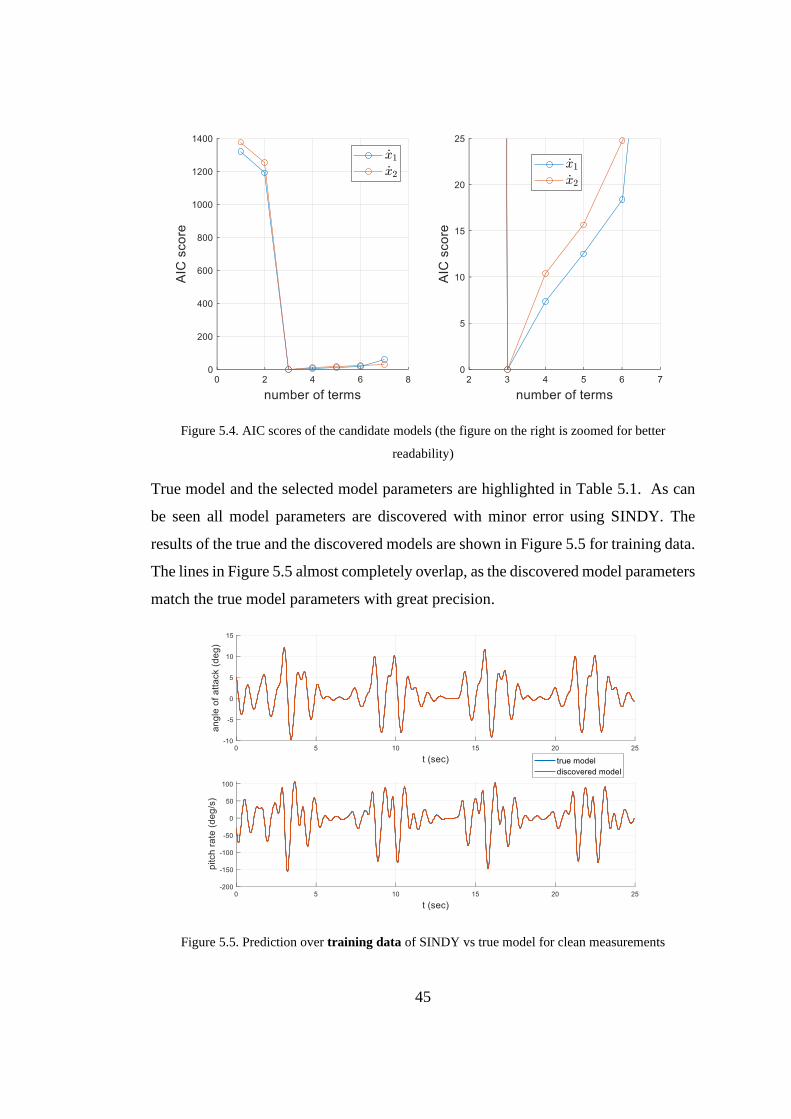
45
Figure 5.4. AIC scores of the candidate models (the figure on the right is zoomed for better
readability)
True model and the selected model parameters are highlighted in Table 5.1. As can
be seen all model parameters are discovered with minor error using SINDY. The
results of the true and the discovered models are shown in Figure 5.5 for training data.
The lines in Figure 5.5 almost completely overlap, as the discovered model parameters
match the true model parameters with great precision.
Figure 5.5. Prediction over training data of SINDY vs true model for clean measurements
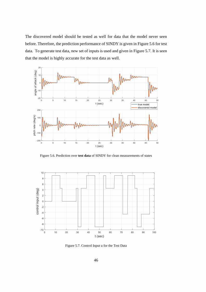
46
The discovered model should be tested as well for data that the model never seen
before. Therefore, the prediction performance of SINDY is given in Figure 5.6 for test
data. To generate test data, new set of inputs is used and given in Figure 5.7. It is seen
that the model is highly accurate for the test data as well.
Figure 5.6. Prediction over test data of SINDY for clean measurements of states
Figure 5.7. Control Input u for the Test Data
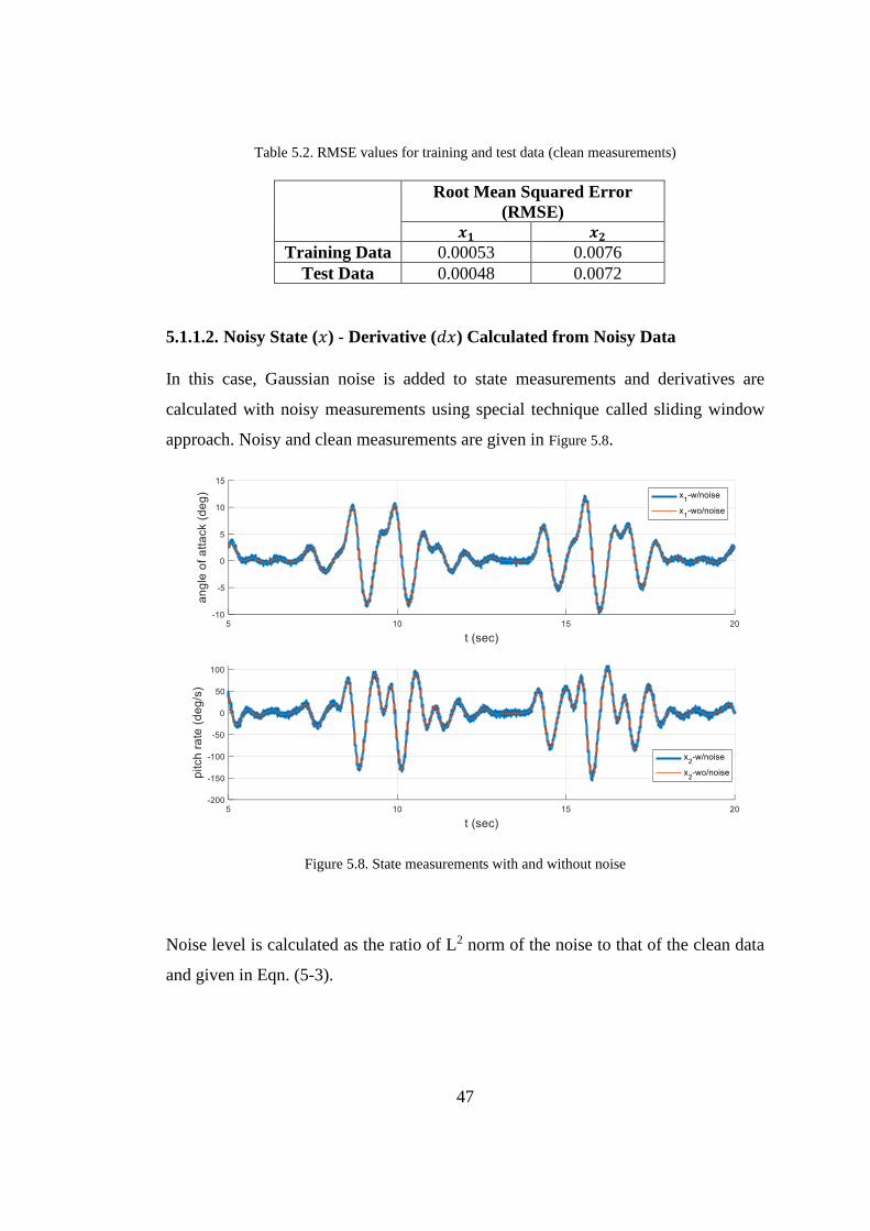
47
Table 5.2. RMSE values for training and test data (clean measurements)
Root Mean Squared Error
(RMSE)
𝒙𝟏 𝒙𝟐
Training Data 0.00053 0.0076
Test Data 0.00048 0.0072
5.1.1.2. Noisy State (𝑥) - Derivative (𝑑𝑥) Calculated from Noisy Data
In this case, Gaussian noise is added to state measurements and derivatives are
calculated with noisy measurements using special technique called sliding window
approach. Noisy and clean measurements are given in Figure 5.8.
Figure 5.8. State measurements with and without noise
Noise level is calculated as the ratio of L2 norm of the noise to that of the clean data
and given in Eqn. (5-3).

48
𝑛𝑜𝑖𝑠𝑒𝑙𝑒𝑣𝑒𝑙(%) =
‖𝑥𝑛𝑜𝑖𝑠𝑦 − 𝑥𝑐𝑙𝑒𝑎𝑛‖2
‖𝑥𝑐𝑙𝑒𝑎𝑛‖2𝑥100
(5-3)
Two noise levels (moderate and high) are used and given in Table 5.3.
Table 5.3. Noise levels for Linear Missile Dynamics
Noise Level (%) of
𝒙𝟏
Noise Level (%) of 𝒙𝟐
Clean 0 0
Moderate 6.0 7.7
High 18.1 23.0
.
Polynomial orders up to 3 is used to construct the library functions. Number of terms
in the discovered model is restricted between 1 to 7. All the models that SINDY
generated are given in Table 5.4.

49
Table 5.4. Candidate models that SINDY generates (moderate noise level)
Number of Terms in the Discovered Model
True
Model 1 2 3 4 5 6 7
�̇�𝟏
𝒙𝟏 -0.4382 0 -0.4413 -0.43828 -0.43999 -0.45161 -0.45144 -0.45621
𝒙𝟐 0.5392 0.532667 0.5356 0.535711 0.535669 0.536512 0.536491 0.53633
𝒖 -0.0243 0 0 0 0 0 0 0
𝒙𝟏𝟐 0 0 0 0 0 0 0 0
𝒙𝟏𝒙𝟐 0 0 0 0 0 0 0 0
𝒙𝟏𝒖 0 0 0 0 0 0 0 0
𝒙𝟐𝟐 0 0 0 0 0 0 0 0
𝒙𝟐𝒖 0 0 0 0 0 0 0 -0.13134
𝒖𝟐 0 0 0 0 0 0 0 0
𝒙𝟏𝟑 0 0 0 0 0 0 0 0
𝒙𝟏𝟐𝒙𝟐 0 0 0 0 0 0 0 0
𝒙𝟏𝟐𝒖 0 0 0 0 0 0 0 0
𝒙𝟏𝒙𝟐𝟐 0 0 0 0 0 0 0 0
𝒙𝟏𝒙𝟐𝒖 0 0 0 0 0 -0.85899 -0.81243 -1.40003
𝒙𝟏𝒖𝟐 0 0 0 0 0.767156 9.595147 9.359713 15.15915
𝒙𝟐𝟑 0 0 0 0 0 0 0 0
𝒙𝟐𝟐𝒖 0 0 0 0 0 0 0 0
𝒙𝟐𝒖𝟐 0 0 0 0 0 0 -0.03851 1.064786
𝒖𝟑 0 0 0 -0.35735 -0.77426 -3.36561 -3.1842 -6.5649
�̇�𝟐
𝒙𝟏 -122.5085 -67.5105 -119.062 -121.647 -121.172 -121.085 -120.065 -120.062
𝒙𝟐 -1.0823 0 0 -1.06267 -1.06291 -1.06275 -1.06738 -1.07369
𝒖 102.7949 0 95.55336 101.9802 99.95954 99.60682 96.70618 96.73651
𝒙𝟏𝟐 0 0 0 0 0 0 -8.1123 -11.6288
𝒙𝟏𝒙𝟐 0 0 0 0 0 0 0 0
𝒙𝟏𝒖 0 0 0 0 0 0 0 13.93773
𝒙𝟐𝟐 0 0 0 0 0 0 0 0
𝒙𝟐𝒖 0 0 0 0 0 0 0 0
𝒖𝟐 0 0 0 0 11.65835 20.97148 65.26909 54.83435
𝒙𝟏𝟑 0 0 0 0 0 0 0 0
𝒙𝟏𝟐𝒙𝟐 0 0 0 0 0 0 0 0
𝒙𝟏𝟐𝒖 0 0 0 0 0 0 0 0
𝒙𝟏𝒙𝟐𝟐 0 0 0 0 0 0 0 0
𝒙𝟏𝒙𝟐𝒖 0 0 0 0 0 0 0 0
𝒙𝟏𝒖𝟐 0 0 0 0 0 0 0 0
𝒙𝟐𝟑 0 0 0 0 0 0 0 0
𝒙𝟐𝟐𝒖 0 0 0 0 0 0 0 0
𝒙𝟐𝒖𝟐 0 0 0 0 0 0 0 0
𝒖𝟑 0 0 0 0 0 -43.6794 -197.461 -178.765
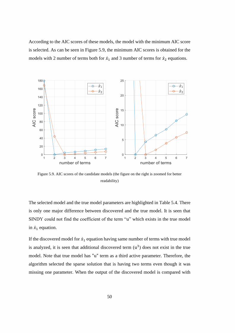
50
According to the AIC scores of these models, the model with the minimum AIC score
is selected. As can be seen in Figure 5.9, the minimum AIC scores is obtained for the
models with 2 number of terms both for �̇�1 and 3 number of terms for �̇�2 equations.
Figure 5.9. AIC scores of the candidate models (the figure on the right is zoomed for better
readability)
The selected model and the true model parameters are highlighted in Table 5.4. There
is only one major difference between discovered and the true model. It is seen that
SINDY could not find the coefficient of the term “u” which exists in the true model
in �̇�1 equation.
If the discovered model for �̇�1 equation having same number of terms with true model
is analyzed, it is seen that additional discovered term (u3) does not exist in the true
model. Note that true model has "u" term as a third active parameter. Therefore, the
algorithm selected the sparse solution that is having two terms even though it was
missing one parameter. When the output of the discovered model is compared with
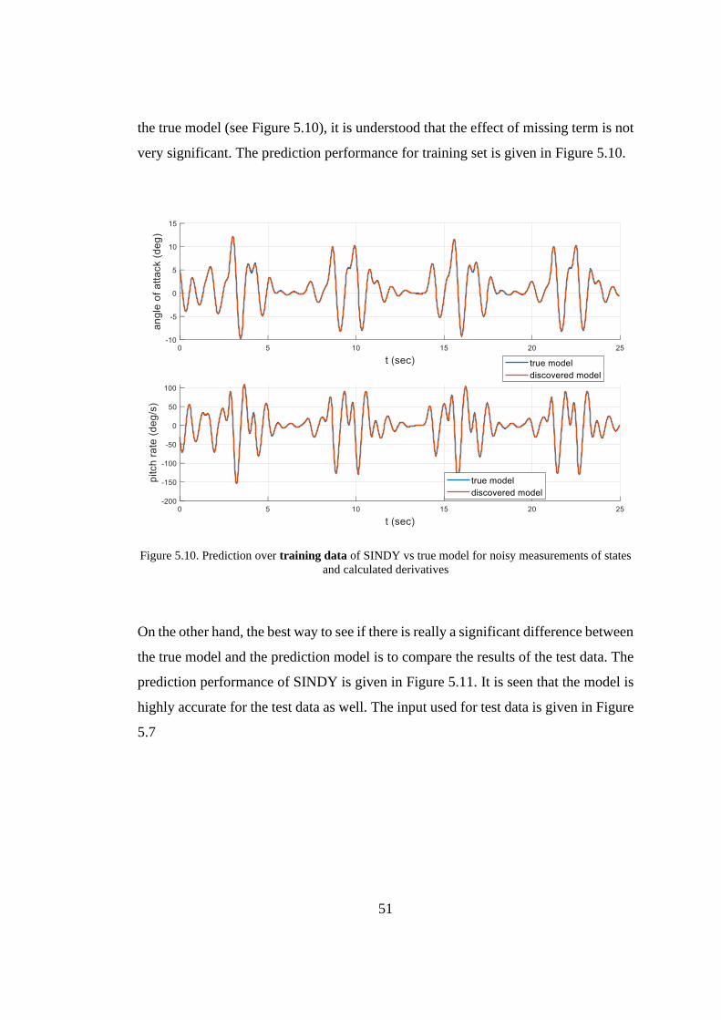
51
the true model (see Figure 5.10), it is understood that the effect of missing term is not
very significant. The prediction performance for training set is given in Figure 5.10.
Figure 5.10. Prediction over training data of SINDY vs true model for noisy measurements of states
and calculated derivatives
On the other hand, the best way to see if there is really a significant difference between
the true model and the prediction model is to compare the results of the test data. The
prediction performance of SINDY is given in Figure 5.11. It is seen that the model is
highly accurate for the test data as well. The input used for test data is given in Figure
5.7
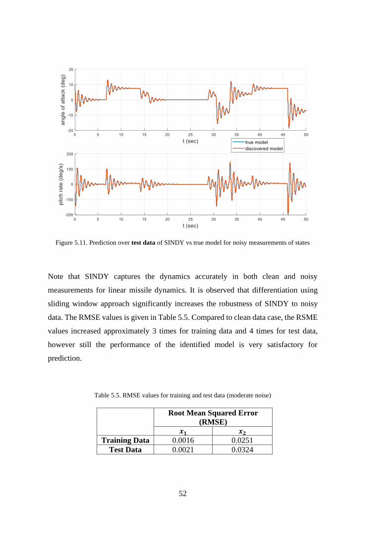
52
Figure 5.11. Prediction over test data of SINDY vs true model for noisy measurements of states
Note that SINDY captures the dynamics accurately in both clean and noisy
measurements for linear missile dynamics. It is observed that differentiation using
sliding window approach significantly increases the robustness of SINDY to noisy
data. The RMSE values is given in Table 5.5. Compared to clean data case, the RSME
values increased approximately 3 times for training data and 4 times for test data,
however still the performance of the identified model is very satisfactory for
prediction.
Table 5.5. RMSE values for training and test data (moderate noise)
Root Mean Squared Error
(RMSE)
𝒙𝟏 𝒙𝟐
Training Data 0.0016 0.0251
Test Data 0.0021 0.0324
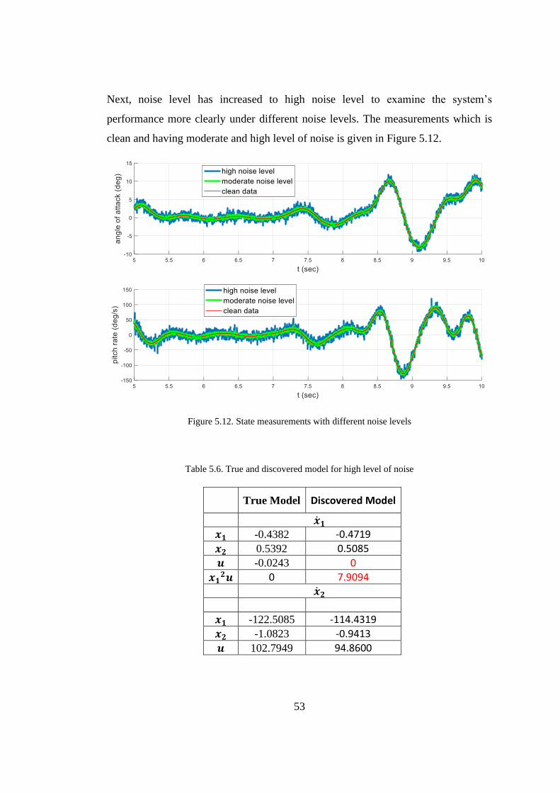
53
Next, noise level has increased to high noise level to examine the system’s
performance more clearly under different noise levels. The measurements which is
clean and having moderate and high level of noise is given in Figure 5.12.
Figure 5.12. State measurements with different noise levels
Table 5.6. True and discovered model for high level of noise
True Model Discovered Model
�̇�𝟏 𝒙𝟏 -0.4382 -0.4719
𝒙𝟐 0.5392 0.5085
𝒖 -0.0243 0
𝒙𝟏𝟐𝒖 0 7.9094 �̇�𝟐
𝒙𝟏 -122.5085 -114.4319
𝒙𝟐 -1.0823 -0.9413
𝒖 102.7949 94.8600
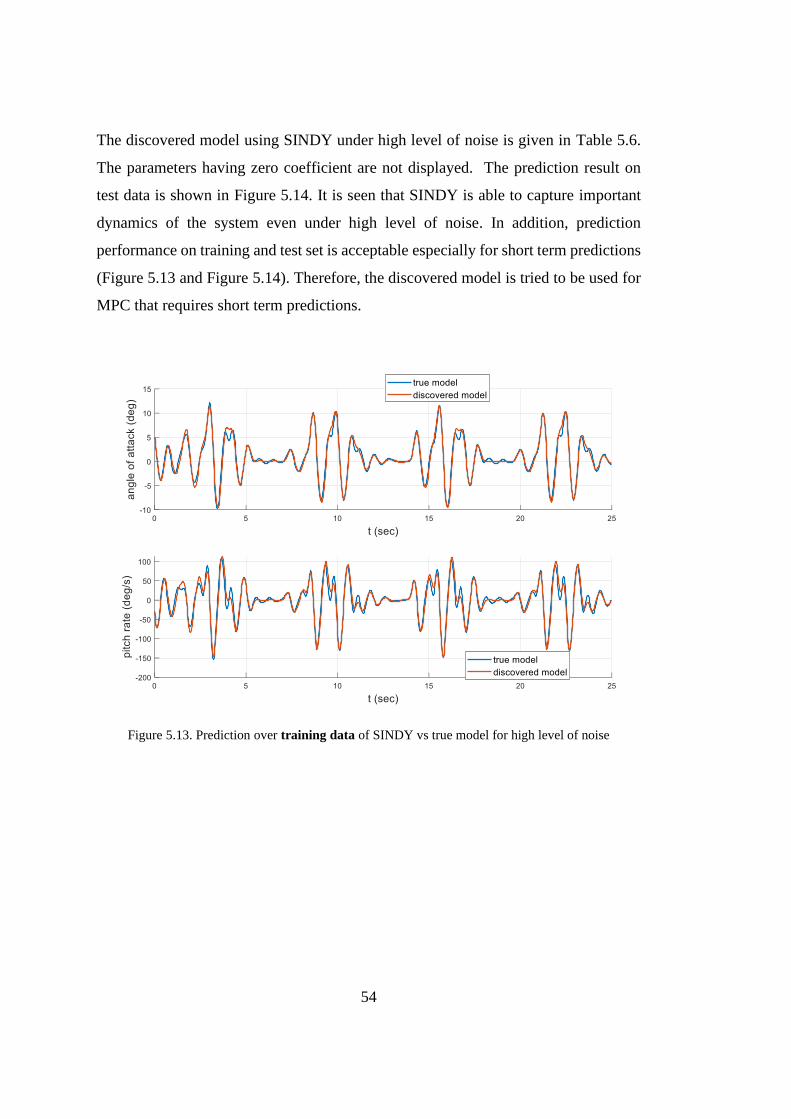
54
The discovered model using SINDY under high level of noise is given in Table 5.6.
The parameters having zero coefficient are not displayed. The prediction result on
test data is shown in Figure 5.14. It is seen that SINDY is able to capture important
dynamics of the system even under high level of noise. In addition, prediction
performance on training and test set is acceptable especially for short term predictions
(Figure 5.13 and Figure 5.14). Therefore, the discovered model is tried to be used for
MPC that requires short term predictions.
Figure 5.13. Prediction over training data of SINDY vs true model for high level of noise
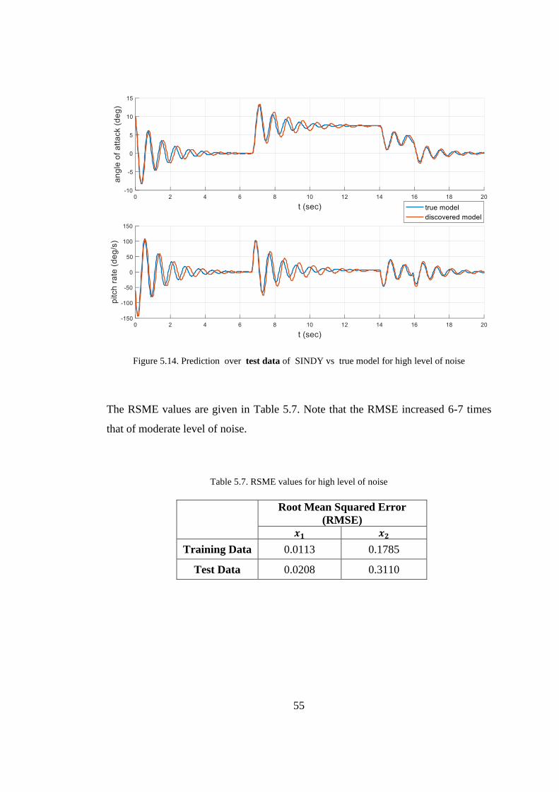
55
Figure 5.14. Prediction over test data of SINDY vs true model for high level of noise
The RSME values are given in Table 5.7. Note that the RMSE increased 6-7 times
that of moderate level of noise.
Table 5.7. RSME values for high level of noise
Root Mean Squared Error
(RMSE)
𝒙𝟏 𝒙𝟐
Training Data 0.0113 0.1785
Test Data 0.0208 0.3110
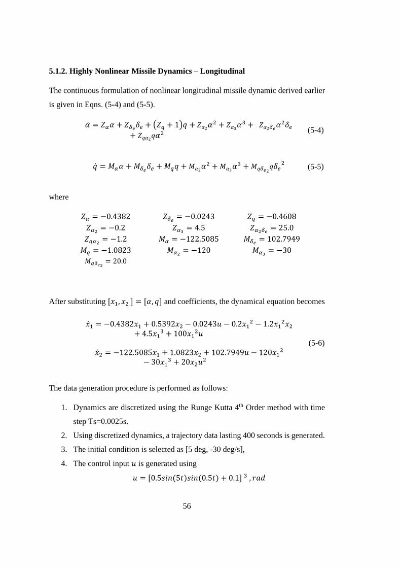
56
5.1.2. Highly Nonlinear Missile Dynamics – Longitudinal
The continuous formulation of nonlinear longitudinal missile dynamic derived earlier
is given in Eqns. (5-4) and (5-5).
�̇� = 𝑍𝛼𝛼 + 𝑍𝛿𝑒
𝛿𝑒 + (𝑍𝑞 + 1)𝑞 + 𝑍𝛼2𝛼2 + 𝑍𝛼3
𝛼3 + 𝑍𝛼2𝛿𝑒𝛼2𝛿𝑒
+ 𝑍𝑞𝛼2𝑞𝛼2
(5-4)
�̇� = 𝑀𝛼𝛼 + 𝑀𝛿𝑒𝛿𝑒 + 𝑀𝑞𝑞 + 𝑀𝛼2
𝛼2 + 𝑀𝛼3𝛼3 + 𝑀𝑞𝛿𝑒2
𝑞𝛿𝑒2 (5-5)
where
𝑍𝛼 = −0.4382 𝑍𝛿𝑒= −0.0243 𝑍𝑞 = −0.4608
𝑍𝛼2= −0.2 𝑍𝛼3
= 4.5 𝑍𝛼2𝛿𝑒= 25.0
𝑍𝑞𝛼2= −1.2 𝑀𝛼 = −122.5085 𝑀𝛿𝑒
= 102.7949
𝑀𝑞 = −1.0823 𝑀𝛼2= −120 𝑀𝛼3
= −30
𝑀𝑞𝛿𝑒2= 20.0
After substituting [𝑥1, 𝑥2 ] = [𝛼, 𝑞] and coefficients, the dynamical equation becomes
�̇�1 = −0.4382𝑥1 + 0.5392𝑥2 − 0.0243𝑢 − 0.2𝑥12 − 1.2𝑥1
2𝑥2
+ 4.5𝑥13 + 100𝑥1
2𝑢
�̇�2 = −122.5085𝑥1 + 1.0823𝑥2 + 102.7949𝑢 − 120𝑥12
− 30𝑥13 + 20𝑥2𝑢
2
(5-6)
The data generation procedure is performed as follows:
1. Dynamics are discretized using the Runge Kutta 4th Order method with time
step Ts=0.0025s.
2. Using discretized dynamics, a trajectory data lasting 400 seconds is generated.
3. The initial condition is selected as [5 deg, -30 deg/s],
4. The control input 𝑢 is generated using
𝑢 = [0.5𝑠𝑖𝑛(5𝑡)𝑠𝑖𝑛(0.5𝑡) + 0.1] 3 , 𝑟𝑎𝑑
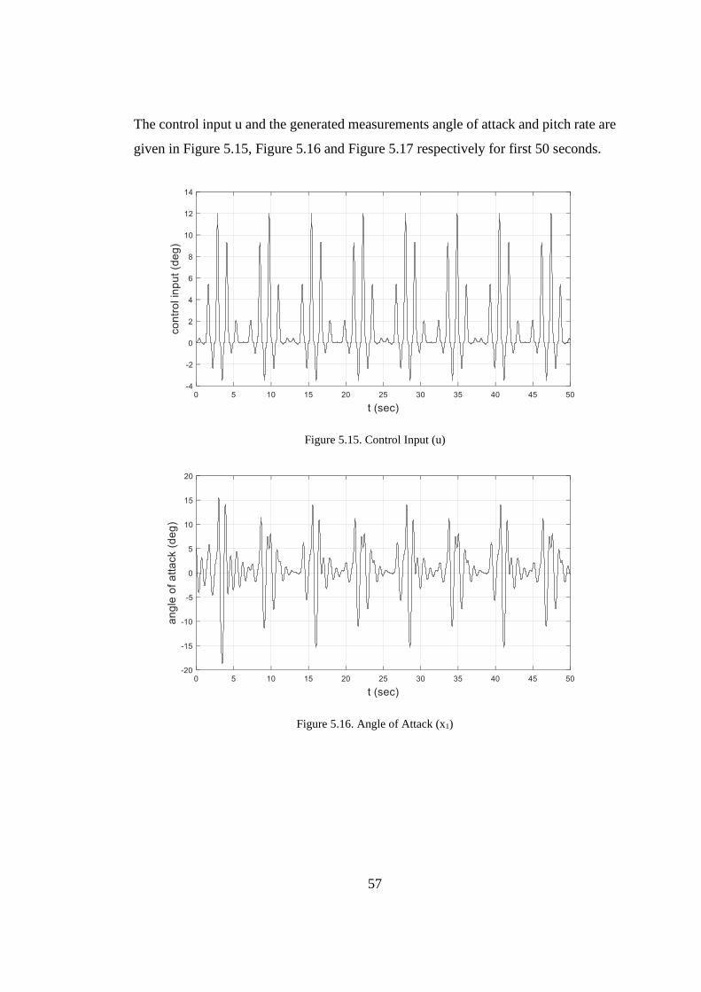
57
The control input u and the generated measurements angle of attack and pitch rate are
given in Figure 5.15, Figure 5.16 and Figure 5.17 respectively for first 50 seconds.
Figure 5.15. Control Input (u)
Figure 5.16. Angle of Attack (x1)

58
Figure 5.17. Pitch Rate (x2)
For the non-linear missile model, 2 cases are studied which are:
1. Clean State (𝑥) - Clean Derivate (�̇�) Case
2. Noisy State (𝑥) - Derivative (�̇�) Calculated from Noisy States Measurements
5.1.2.1. Clean State (𝑥) - Clean Derivative (𝑑𝑥) Case
In this case, it is assumed that states are measured without noise and derivatives are
measured directly or calculated from clean state measurements perfectly.
Polynomial orders up to 3 is used to construct the library functions. Number of terms
in the discovered model is restricted between 1 to 10. All the models that SINDY
generated are given in Table 5.8 and Table 5.9. According to the AIC scores of these
models, the model with the minimum AIC score is selected. As can be seen in Figure
5.18, the minimum AIC scores is obtained for the models containing 6 number of
terms for both �̇�1 and �̇�2 equations.

59
Table 5.8. Candidate models that SINDY generates for �̇�1 (clean data)
Table 5.9. Candidate models that SINDY generates for �̇�2 (clean data)
It is obvious that for �̇�1 equation, model having 7 number of terms instead of 6 would
be a better choice (see Table 5.8). However, missing term has little effect on system
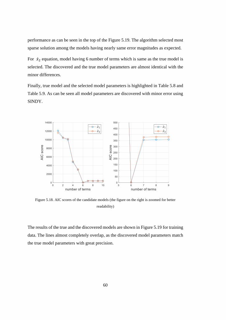
60
performance as can be seen in the top of the Figure 5.19. The algorithm selected most
sparse solution among the models having nearly same error magnitudes as expected.
For �̇�2 equation, model having 6 number of terms which is same as the true model is
selected. The discovered and the true model parameters are almost identical with the
minor differences.
Finally, true model and the selected model parameters is highlighted in Table 5.8 and
Table 5.9. As can be seen all model parameters are discovered with minor error using
SINDY.
Figure 5.18. AIC scores of the candidate models (the figure on the right is zoomed for better
readability)
The results of the true and the discovered models are shown in Figure 5.19 for training
data. The lines almost completely overlap, as the discovered model parameters match
the true model parameters with great precision.
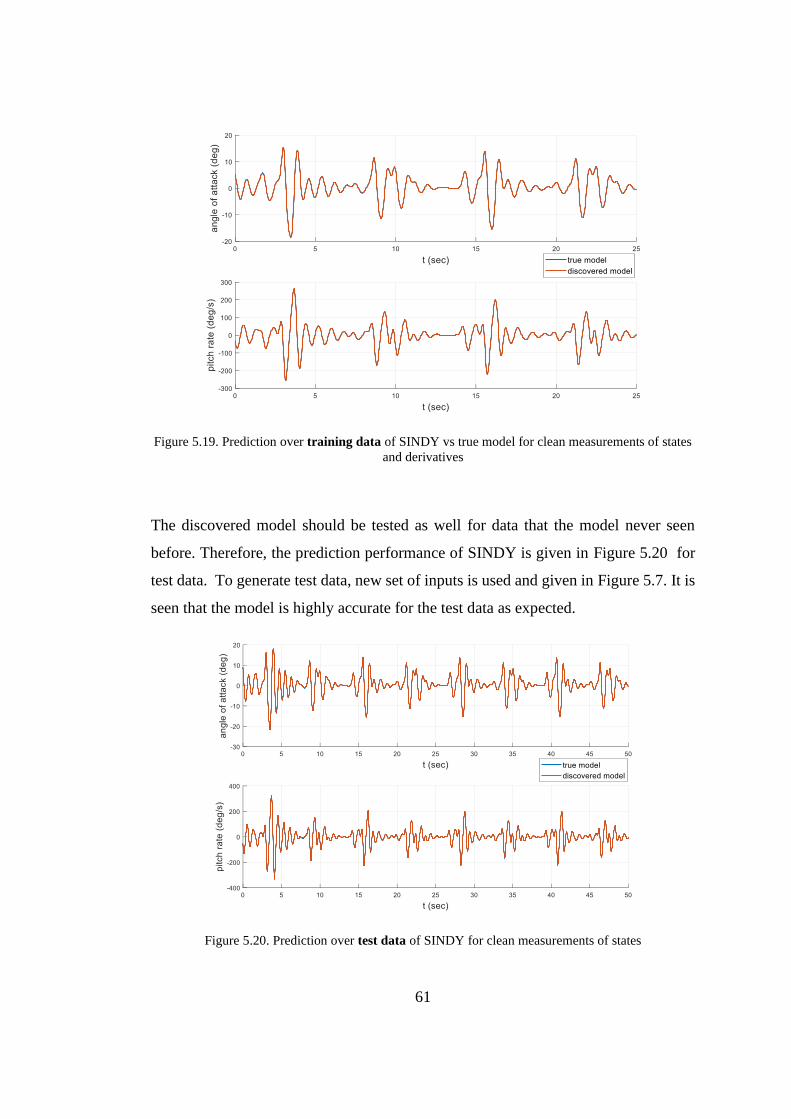
61
Figure 5.19. Prediction over training data of SINDY vs true model for clean measurements of states
and derivatives
The discovered model should be tested as well for data that the model never seen
before. Therefore, the prediction performance of SINDY is given in Figure 5.20 for
test data. To generate test data, new set of inputs is used and given in Figure 5.7. It is
seen that the model is highly accurate for the test data as expected.
Figure 5.20. Prediction over test data of SINDY for clean measurements of states
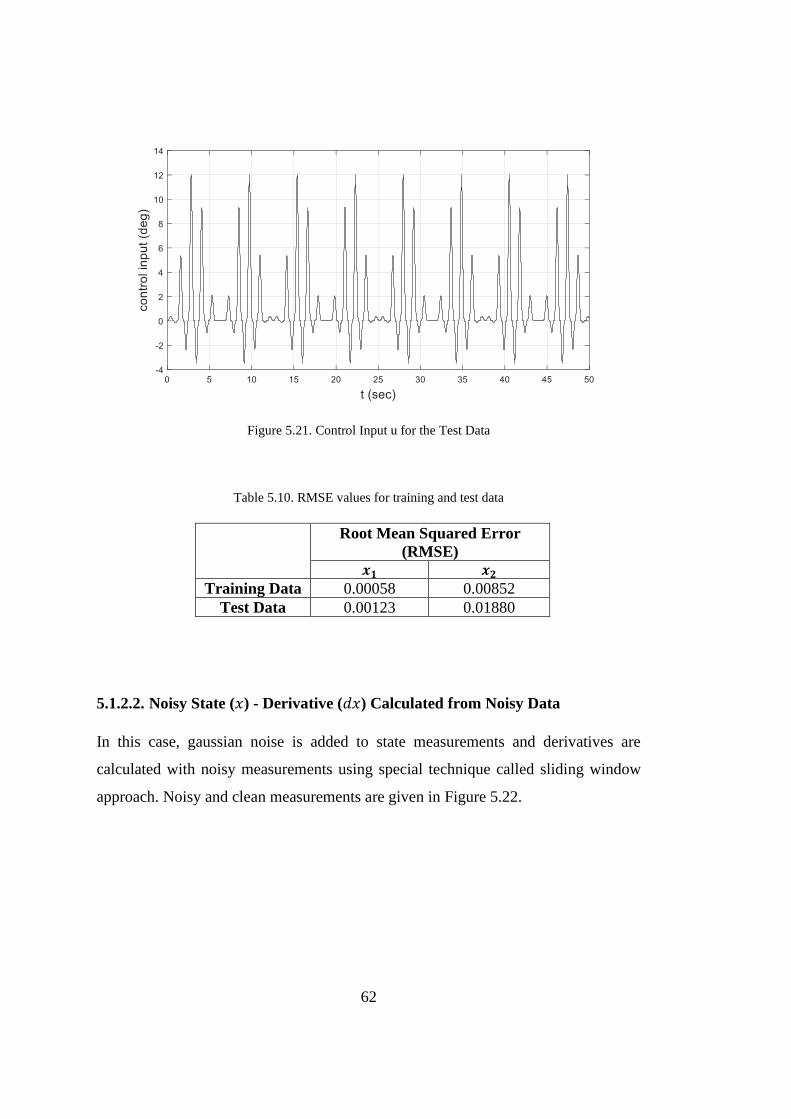
62
Figure 5.21. Control Input u for the Test Data
Table 5.10. RMSE values for training and test data
Root Mean Squared Error
(RMSE)
𝒙𝟏 𝒙𝟐
Training Data 0.00058 0.00852
Test Data 0.00123 0.01880
5.1.2.2. Noisy State (𝑥) - Derivative (𝑑𝑥) Calculated from Noisy Data
In this case, gaussian noise is added to state measurements and derivatives are
calculated with noisy measurements using special technique called sliding window
approach. Noisy and clean measurements are given in Figure 5.22.
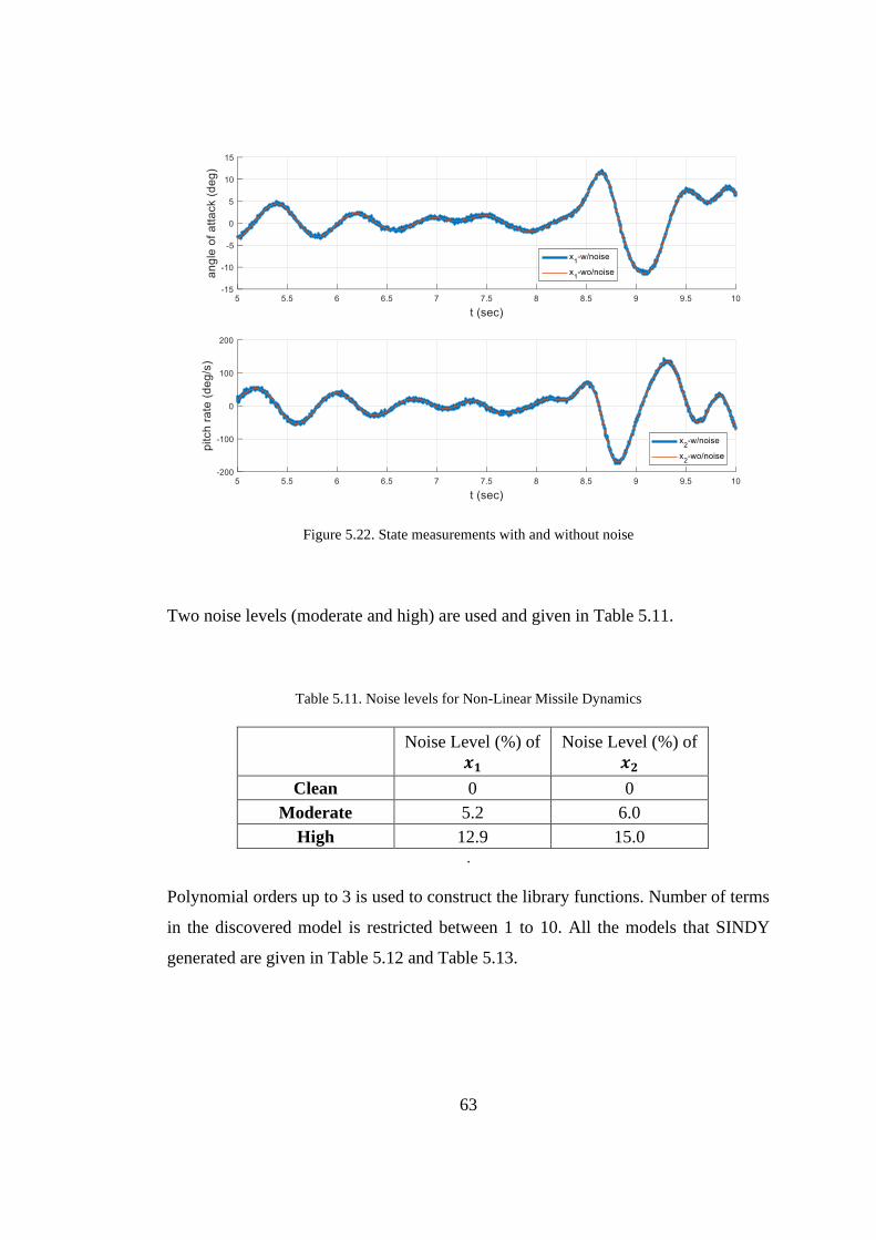
63
Figure 5.22. State measurements with and without noise
Two noise levels (moderate and high) are used and given in Table 5.11.
Table 5.11. Noise levels for Non-Linear Missile Dynamics
Noise Level (%) of
𝒙𝟏
Noise Level (%) of 𝒙𝟐
Clean 0 0
Moderate 5.2 6.0
High 12.9 15.0 .
Polynomial orders up to 3 is used to construct the library functions. Number of terms
in the discovered model is restricted between 1 to 10. All the models that SINDY
generated are given in Table 5.12 and Table 5.13.

64
Table 5.12. Candidate models that SINDY generates for �̇�1 (moderate noise level)
Table 5.13. Candidate models that SINDY generates for �̇�2 (moderate noise level)
Based on the AIC scores of these models, the model having minimum AIC score is
selected. As can be seen in Figure 5.23, the minimum AIC scores is obtained for the
models with 5 number of terms both for �̇�1 and �̇�2 equations.
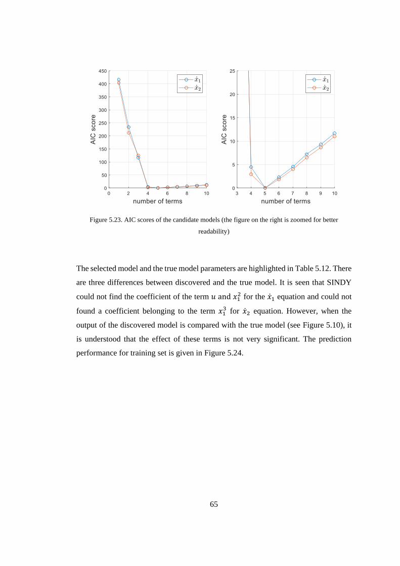
65
Figure 5.23. AIC scores of the candidate models (the figure on the right is zoomed for better
readability)
The selected model and the true model parameters are highlighted in Table 5.12. There
are three differences between discovered and the true model. It is seen that SINDY
could not find the coefficient of the term 𝑢 and 𝑥12 for the �̇�1 equation and could not
found a coefficient belonging to the term 𝑥13 for �̇�2 equation. However, when the
output of the discovered model is compared with the true model (see Figure 5.10), it
is understood that the effect of these terms is not very significant. The prediction
performance for training set is given in Figure 5.24.
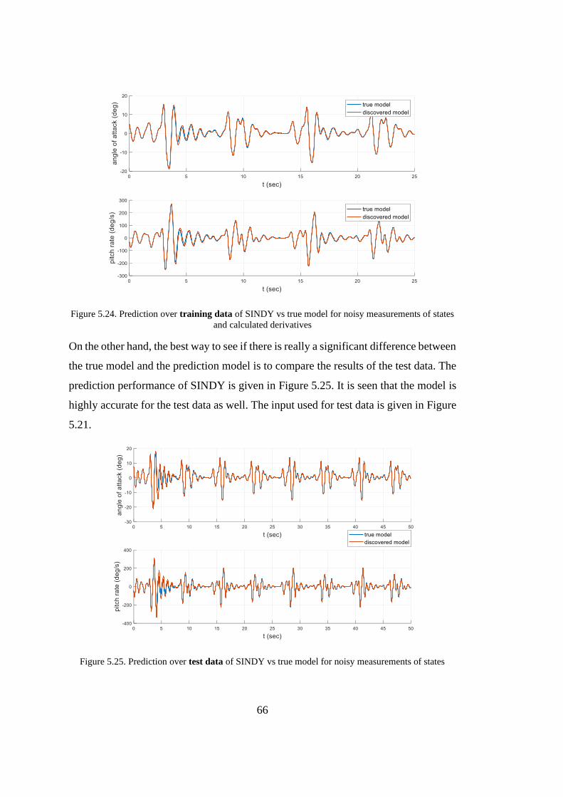
66
Figure 5.24. Prediction over training data of SINDY vs true model for noisy measurements of states
and calculated derivatives
On the other hand, the best way to see if there is really a significant difference between
the true model and the prediction model is to compare the results of the test data. The
prediction performance of SINDY is given in Figure 5.25. It is seen that the model is
highly accurate for the test data as well. The input used for test data is given in Figure
5.21.
Figure 5.25. Prediction over test data of SINDY vs true model for noisy measurements of states
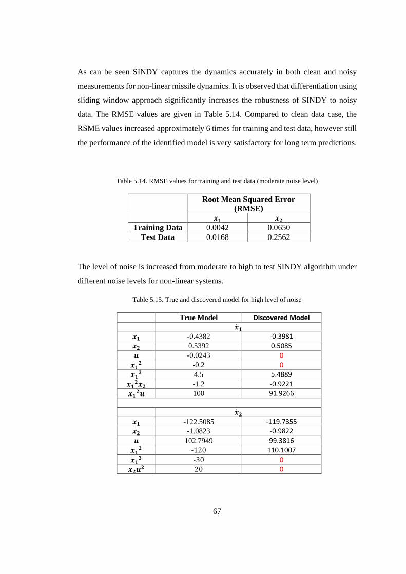
67
As can be seen SINDY captures the dynamics accurately in both clean and noisy
measurements for non-linear missile dynamics. It is observed that differentiation using
sliding window approach significantly increases the robustness of SINDY to noisy
data. The RMSE values are given in Table 5.14. Compared to clean data case, the
RSME values increased approximately 6 times for training and test data, however still
the performance of the identified model is very satisfactory for long term predictions.
Table 5.14. RMSE values for training and test data (moderate noise level)
Root Mean Squared Error
(RMSE)
𝒙𝟏 𝒙𝟐
Training Data 0.0042 0.0650
Test Data 0.0168 0.2562
The level of noise is increased from moderate to high to test SINDY algorithm under
different noise levels for non-linear systems.
Table 5.15. True and discovered model for high level of noise
True Model Discovered Model
�̇�𝟏 𝒙𝟏 -0.4382 -0.3981
𝒙𝟐 0.5392 0.5085
𝒖 -0.0243 0
𝒙𝟏𝟐 -0.2 0
𝒙𝟏𝟑 4.5 5.4889
𝒙𝟏𝟐𝒙𝟐 -1.2 -0.9221
𝒙𝟏𝟐𝒖 100 91.9266
�̇�𝟐
𝒙𝟏 -122.5085 -119.7355
𝒙𝟐 -1.0823 -0.9822
𝒖 102.7949 99.3816
𝒙𝟏𝟐 -120 110.1007
𝒙𝟏𝟑 -30 0
𝒙𝟐𝒖𝟐 20 0
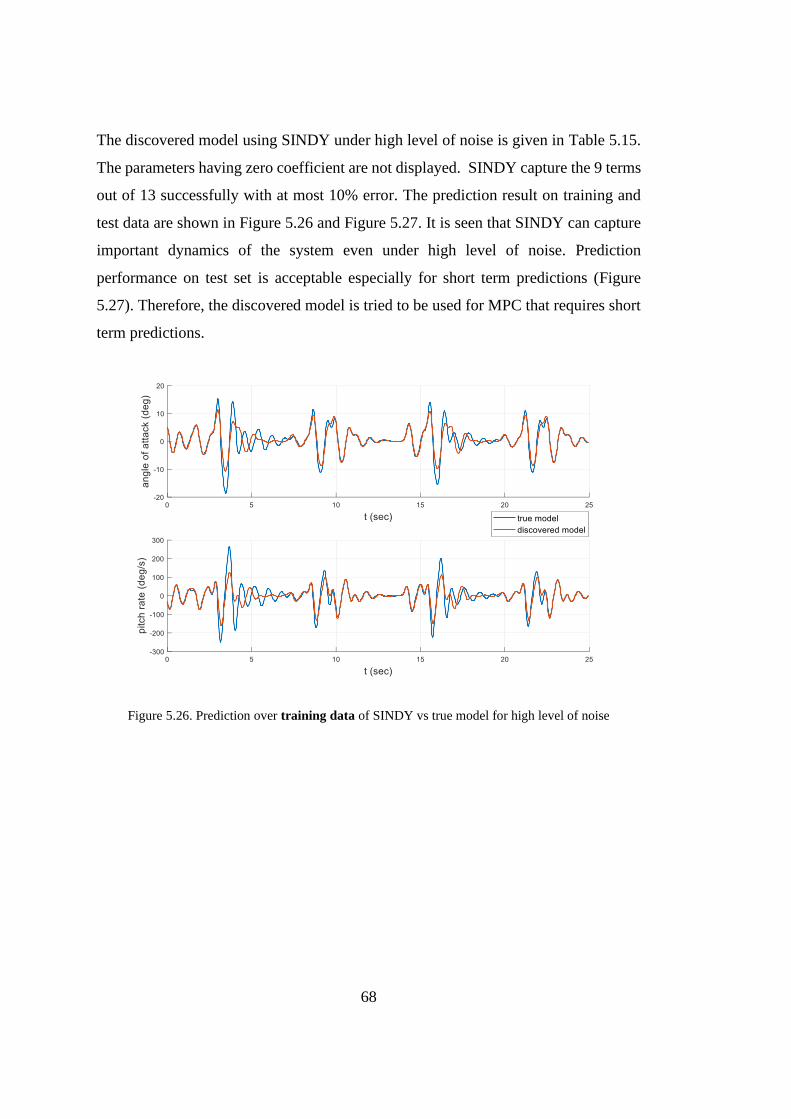
68
The discovered model using SINDY under high level of noise is given in Table 5.15.
The parameters having zero coefficient are not displayed. SINDY capture the 9 terms
out of 13 successfully with at most 10% error. The prediction result on training and
test data are shown in Figure 5.26 and Figure 5.27. It is seen that SINDY can capture
important dynamics of the system even under high level of noise. Prediction
performance on test set is acceptable especially for short term predictions (Figure
5.27). Therefore, the discovered model is tried to be used for MPC that requires short
term predictions.
Figure 5.26. Prediction over training data of SINDY vs true model for high level of noise
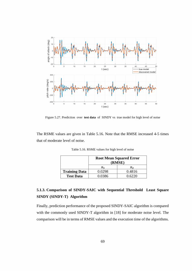
69
Figure 5.27. Prediction over test data of SINDY vs true model for high level of noise
The RSME values are given in Table 5.16. Note that the RMSE increased 4-5 times
that of moderate level of noise.
Table 5.16. RSME values for high level of noise
Root Mean Squared Error
(RMSE)
𝒙𝟏 𝒙𝟐
Training Data 0.0298 0.4816
Test Data 0.0386 0.6220
5.1.3. Comparison of SINDY-SAIC with Sequential Threshold Least Square
SINDY (SINDY-T) Algorithm
Finally, prediction performance of the proposed SINDY-SAIC algorithm is compared
with the commonly used SINDY-T algorithm in [18] for moderate noise level. The
comparison will be in terms of RMSE values and the execution time of the algorithms.

70
The discovered model parameters of both methods and their percent error in model
parameters are given in Table 5.17 and Table 5.18 for �̇�1 and �̇�2 equations
respectively. It is seen that both methods successfully discovered the important
dynamics. However, for the examined dynamical system, SINDY- SAIC has slightly
lover percent error in some of the coefficients for �̇�2 equation. Furthermore, SINDY-
SAIC captures the dynamics related to 𝑥2𝑢2 term successfully whereas SINDY-T does
not.
Table 5.17. Comparison of SINDY methods for �̇�1
�̇�𝟏 % Error in the Parameters
True Model SINDY-SAIC SINDY-T SINDY-SAIC SINDY-T
𝒙𝟏 -0.4382 -0.4454 -0.4454 1.64 1.65
𝒙𝟐 0.5392 0.5368 0.5368 0.45 0.45
𝒖 -0.0243 0 0 100.00 100.00
𝒙𝟏𝟐 -0.2000 0 0 100.00 100.00
𝒙𝟏𝒙𝟐 0 0 0
𝒙𝟏𝒖 0 0 0
𝒙𝟐𝟐 0 0 0
𝒖𝟐 0 0 0
𝒙𝟏𝟑 4.5000 5.7781 5.7781 28.40 28.40
𝒙𝟏𝟐𝒙𝟐 -1.2000 -1.1508 -1.1508 4.10 4.10
𝒙𝟏𝟐𝒖 100.0000 95.9496 95.9496 4.05 4.05
𝒙𝟏𝒙𝟐𝟐 0 0 0
𝒙𝟏𝒙𝟐𝒖 0 0 0
𝒙𝟏𝒖𝟐 0 0 0
𝒙𝟐𝟑 0 0 0
𝒙𝟐𝟐𝒖 0 0 0
𝒙𝟐𝒖𝟐 0 0 0
𝒖𝟑 0 0 0

71
Table 5.18. Comparison of SINDY methods for �̇�2
�̇�𝟏 % Error in the Parameters
True Model SINDY-SAIC SINDY-T SINDY-SAIC SINDY-T
𝒙𝟏 -122.5081 -122.9884 -122.9857 0.39 0.39
𝒙𝟐 -1.0823 -1.0666 -1.0204 1.45 5.72
𝒖 102.7944 102.5359 102.9230 0.25 0.13
𝒙𝟏𝟐 -120.0000 -117.9593 -117.1365 1.70 2.39
𝒙𝟏𝒙𝟐 0 0 0
𝒙𝟏𝒖 0 0 0
𝒙𝟐𝟐 0 0 0
𝒙𝟐𝒖 0 0 0
𝒖𝟐 0 0 0
𝒙𝟏𝟑 -30.0000 0 0
𝒙𝟏𝟐𝒙𝟐 0 0 0
𝒙𝟏𝟐𝒖 0 0 0
𝒙𝟏𝒙𝟐𝟐 0 0 0
𝒙𝟏𝒙𝟐𝒖 0 0 0
𝒙𝟏𝒖𝟐 0 0 0
𝒙𝟐𝟑 0 0 0
𝒙𝟐𝟐𝒖 0 0 0
𝒙𝟐𝒖𝟐 20.0000 20.0004 0 0.00 100.00
𝒖𝟑 0 0 0
The RMSE values of both algorithms are given in Table 5.19. It is seen that SINDY-
SAIC algorithm has lover RSME values than the SINDY-T algorithm. This result is
consistent with that the later one captured one less term than the former.
Table 5.19. RSME values of SINDY methods
Root Mean Squared Error
(RMSE)
𝒙𝟏 𝒙𝟐 SINDY-SAIC SINDY-T SINDY-SAIC SINDY-T
Training Data 0.0042 0.0048 0.0650 0.0735
Test Data 0.0168 0.0371 0.2565 0. 4807
The time of execution for methods are measured and observed that SINDY-SAIC
converges 5.6 faster than the SINDY-T. SINDY-SAIC algorithm produces a much

72
smaller number of candidate models and hence execution time is much shorter. In this
example, SINDY-SAIC algorithm generated 10 candidate models, while the SINDY-
T algorithm generated 56 candidate models. All the time difference come from the
number of candidate models generated by methods.
5.2. Control Performance Comparison
In this section control performances of the discovered models and the different kind
of controller are to be analyzed. The cases studied are given as follows.
1. Linear Missile Model Control (with clean and noisy measurement)
1. MPC
2. State Feedback (SF)
2. Non-Linear Missile Model (with clean and noisy measurement)
1. Non-linear MPC
2. State Feedback (SF)
3. MPC
The performances are to be compared in terms of The Tracking Error (TE), Control
Expenditure (CE) and Control Rate Expenditure (CRE) and the definitions are given
in Eqn. (5-7).
𝑇𝑟𝑎𝑐𝑘𝑖𝑛𝑔 𝐸𝑟𝑟𝑜𝑟 ∶= ∫ |(𝛼 − 𝛼𝑟𝑒𝑓)|𝑇𝑠𝑒𝑡𝑡𝑙𝑖𝑛𝑔
0
𝐶𝑜𝑛𝑡𝑟𝑜𝑙 𝐸𝑥𝑝𝑎𝑛𝑑𝑖𝑡𝑢𝑟𝑒 ∶= ∫ |𝛿|𝑇𝑠𝑒𝑡𝑡𝑙𝑖𝑛𝑔
0
𝐶𝑜𝑛𝑡𝑟𝑜𝑙 𝑅𝑎𝑡𝑒 𝐸𝑥𝑝𝑎𝑛𝑑𝑖𝑡𝑢𝑟𝑒 ∶= ∫ |�̇�|𝑇𝑠𝑒𝑡𝑡𝑙𝑖𝑛𝑔
0
(5-7)

73
5.2.1. Control Performance Comparison for Linear Missile Model
In this section, discovered model is used to control the linear missile model using MPC
and state feedback (SF) control methods. In MPC discovered model is used for
prediction whereas in state feedback control it is used during the pole placement
procedure. Both control methods are compared for clean and noisy measurements. The
true model and the previously discovered models for clean and noisy measurements
are given in Table 5.20.
Table 5.20. Discovered models using SINDY
True model Model-1
(Clean Measurement) Model-2
(Moderate Noise) Model-3
(High Noise)
�̇�𝟏
𝒙𝟏 -0.4382 -0.4382 -0.4413 -0.4719
𝒙𝟐 0.5392 0.5392 0.5355 0.5085
𝒖 -0.0243 -0.0243 0 0
�̇�𝟐
𝒙𝟏 -122.5085 -122.5085 -121.6470 -114.4319
𝒙𝟐 -1.0823 -1.0823 -1.0627 -0.9413
𝒖 102.7949 102.7949 101.9802 94.8600
MPC and State Feedback (SF) design parameters are given in Table 5.21 and Table
5.22 respectively.
Table 5.21. MPC design parameters for linear system
MPC Design Parameters Values
Sample Time (Ts) 0.025
Prediction Horizon (Hp) 35
Control Horizon (Hm) 4
Output Weight (Q) 1
Input Rate Weight (R) 2.5
Input Constraints [-15, 15] deg
Input Rate Constraints [-250, 250] deg/s
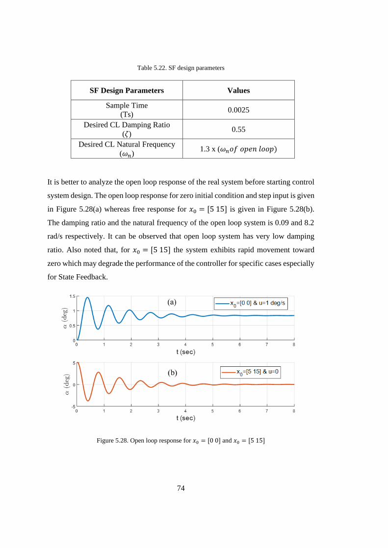
74
Table 5.22. SF design parameters
SF Design Parameters Values
Sample Time
(Ts) 0.0025
Desired CL Damping Ratio
(𝜁) 0.55
Desired CL Natural Frequency
(𝜔𝑛) 1.3 x (𝜔𝑛𝑜𝑓 𝑜𝑝𝑒𝑛 𝑙𝑜𝑜𝑝)
It is better to analyze the open loop response of the real system before starting control
system design. The open loop response for zero initial condition and step input is given
in Figure 5.28(a) whereas free response for 𝑥0 = [5 15] is given in Figure 5.28(b).
The damping ratio and the natural frequency of the open loop system is 0.09 and 8.2
rad/s respectively. It can be observed that open loop system has very low damping
ratio. Also noted that, for 𝑥0 = [5 15] the system exhibits rapid movement toward
zero which may degrade the performance of the controller for specific cases especially
for State Feedback.
Figure 5.28. Open loop response for 𝑥0 = [0 0] and 𝑥0 = [5 15]
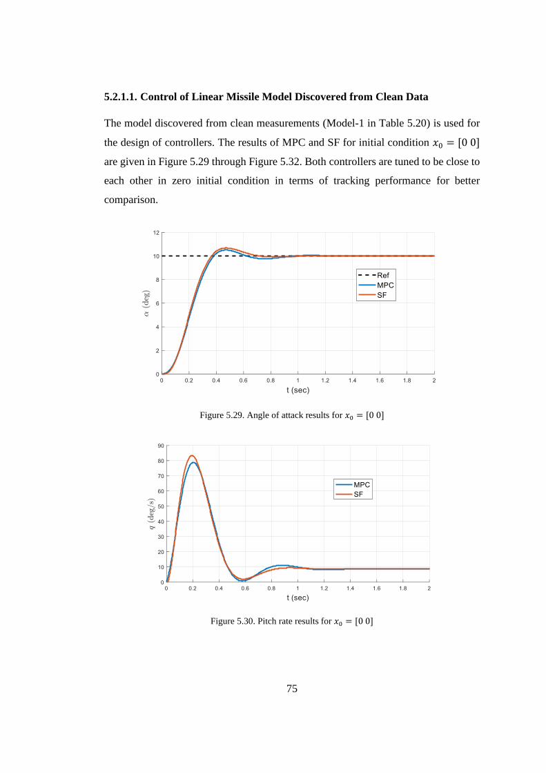
75
5.2.1.1. Control of Linear Missile Model Discovered from Clean Data
The model discovered from clean measurements (Model-1 in Table 5.20) is used for
the design of controllers. The results of MPC and SF for initial condition 𝑥0 = [0 0]
are given in Figure 5.29 through Figure 5.32. Both controllers are tuned to be close to
each other in zero initial condition in terms of tracking performance for better
comparison.
Figure 5.29. Angle of attack results for 𝑥0 = [0 0]
Figure 5.30. Pitch rate results for 𝑥0 = [0 0]
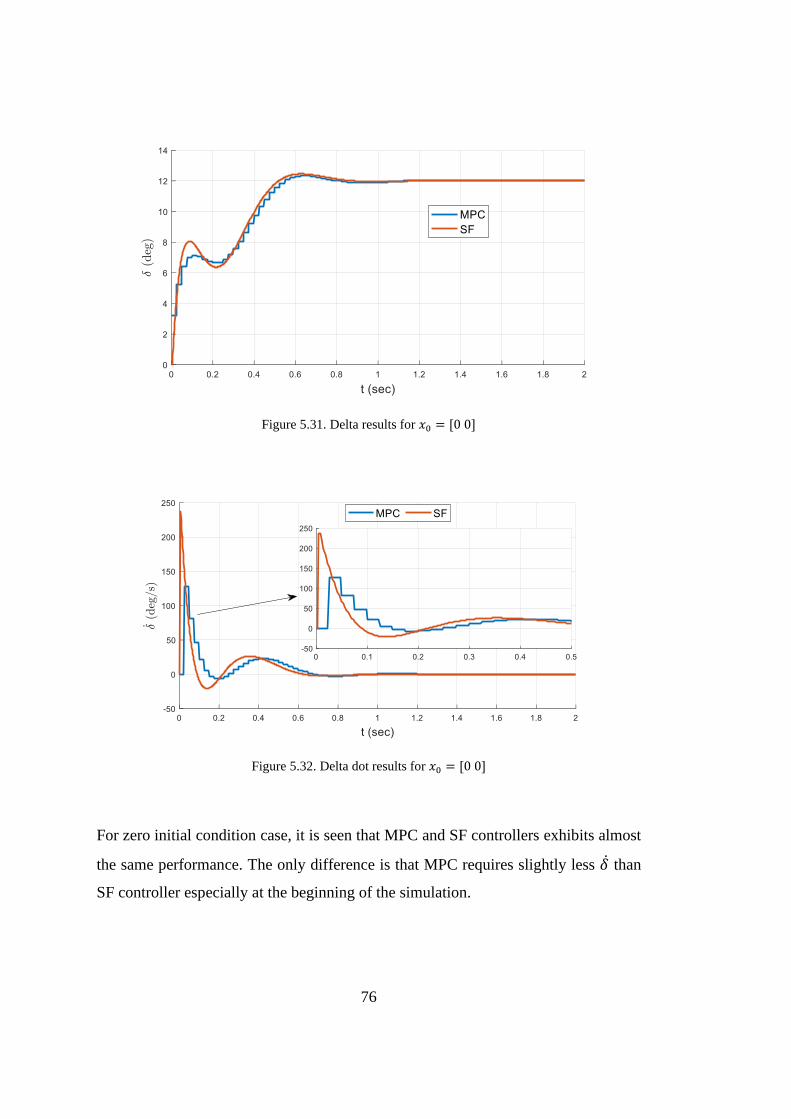
76
Figure 5.31. Delta results for 𝑥0 = [0 0]
Figure 5.32. Delta dot results for 𝑥0 = [0 0]
For zero initial condition case, it is seen that MPC and SF controllers exhibits almost
the same performance. The only difference is that MPC requires slightly less �̇� than
SF controller especially at the beginning of the simulation.
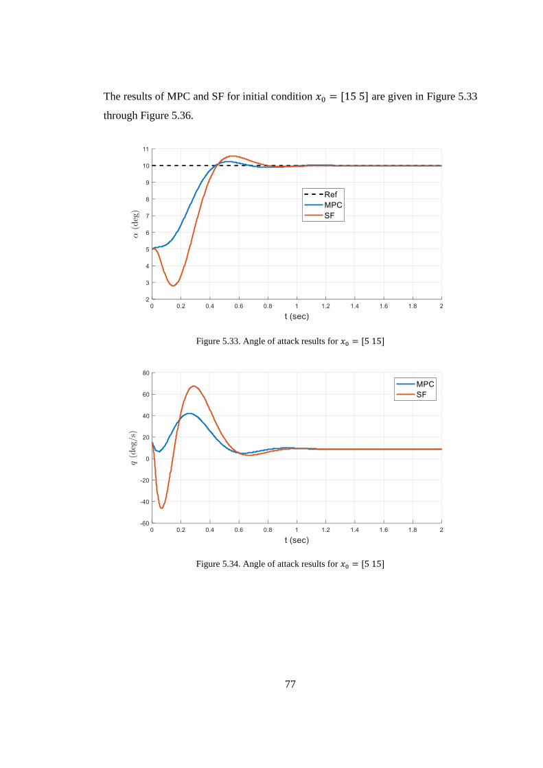
77
The results of MPC and SF for initial condition 𝑥0 = [15 5] are given in Figure 5.33
through Figure 5.36.
Figure 5.33. Angle of attack results for 𝑥0 = [5 15]
Figure 5.34. Angle of attack results for 𝑥0 = [5 15]
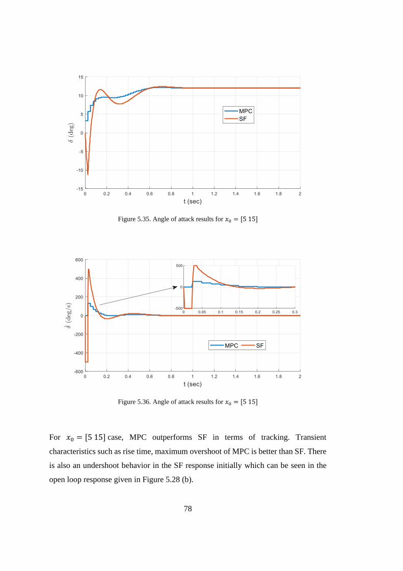
78
Figure 5.35. Angle of attack results for 𝑥0 = [5 15]
Figure 5.36. Angle of attack results for 𝑥0 = [5 15]
For 𝑥0 = [5 15] case, MPC outperforms SF in terms of tracking. Transient
characteristics such as rise time, maximum overshoot of MPC is better than SF. There
is also an undershoot behavior in the SF response initially which can be seen in the
open loop response given in Figure 5.28 (b).
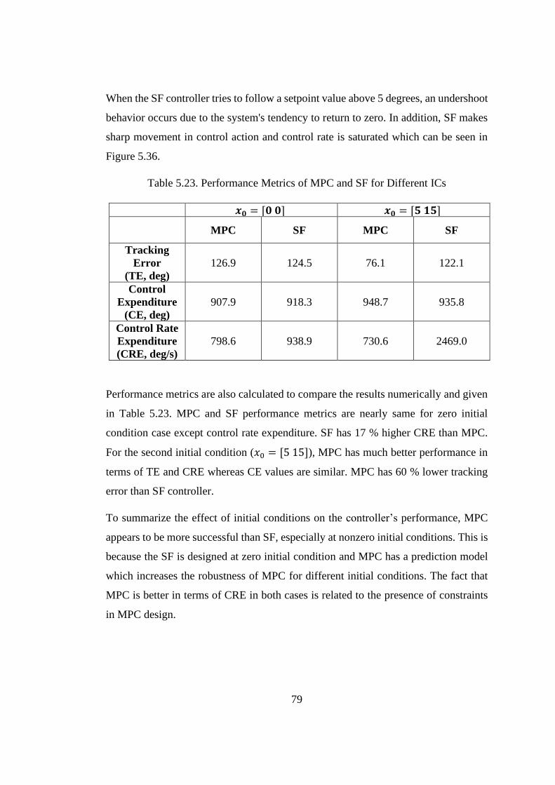
79
When the SF controller tries to follow a setpoint value above 5 degrees, an undershoot
behavior occurs due to the system's tendency to return to zero. In addition, SF makes
sharp movement in control action and control rate is saturated which can be seen in
Figure 5.36.
Table 5.23. Performance Metrics of MPC and SF for Different ICs
𝒙𝟎 = [𝟎 𝟎] 𝒙𝟎 = [𝟓 𝟏𝟓]
MPC SF MPC SF
Tracking
Error
(TE, deg)
126.9 124.5 76.1 122.1
Control
Expenditure
(CE, deg)
907.9 918.3 948.7 935.8
Control Rate
Expenditure
(CRE, deg/s)
798.6 938.9 730.6 2469.0
Performance metrics are also calculated to compare the results numerically and given
in Table 5.23. MPC and SF performance metrics are nearly same for zero initial
condition case except control rate expenditure. SF has 17 % higher CRE than MPC.
For the second initial condition (𝑥0 = [5 15]), MPC has much better performance in
terms of TE and CRE whereas CE values are similar. MPC has 60 % lower tracking
error than SF controller.
To summarize the effect of initial conditions on the controller’s performance, MPC
appears to be more successful than SF, especially at nonzero initial conditions. This is
because the SF is designed at zero initial condition and MPC has a prediction model
which increases the robustness of MPC for different initial conditions. The fact that
MPC is better in terms of CRE in both cases is related to the presence of constraints
in MPC design.
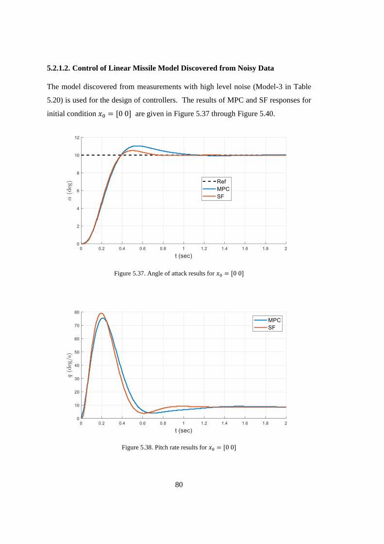
80
5.2.1.2. Control of Linear Missile Model Discovered from Noisy Data
The model discovered from measurements with high level noise (Model-3 in Table
5.20) is used for the design of controllers. The results of MPC and SF responses for
initial condition 𝑥0 = [0 0] are given in Figure 5.37 through Figure 5.40.
Figure 5.37. Angle of attack results for 𝑥0 = [0 0]
Figure 5.38. Pitch rate results for 𝑥0 = [0 0]
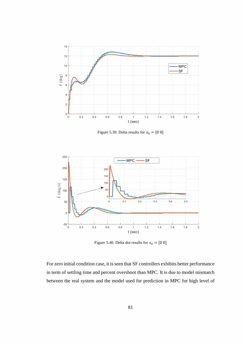
81
Figure 5.39. Delta results for 𝑥0 = [0 0]
Figure 5.40. Delta dot results for 𝑥0 = [0 0]
For zero initial condition case, it is seen that SF controllers exhibits better performance
in term of settling time and percent overshoot than MPC. It is due to model mismatch
between the real system and the model used for prediction in MPC for high level of
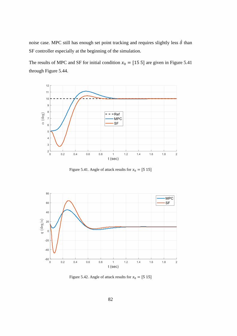
82
noise case. MPC still has enough set point tracking and requires slightly less �̇� than
SF controller especially at the beginning of the simulation.
The results of MPC and SF for initial condition 𝑥0 = [15 5] are given in Figure 5.41
through Figure 5.44.
Figure 5.41. Angle of attack results for 𝑥0 = [5 15]
Figure 5.42. Angle of attack results for 𝑥0 = [5 15]
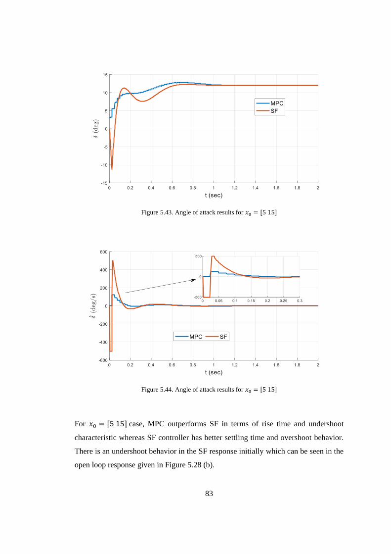
83
Figure 5.43. Angle of attack results for 𝑥0 = [5 15]
Figure 5.44. Angle of attack results for 𝑥0 = [5 15]
For 𝑥0 = [5 15] case, MPC outperforms SF in terms of rise time and undershoot
characteristic whereas SF controller has better settling time and overshoot behavior.
There is an undershoot behavior in the SF response initially which can be seen in the
open loop response given in Figure 5.28 (b).
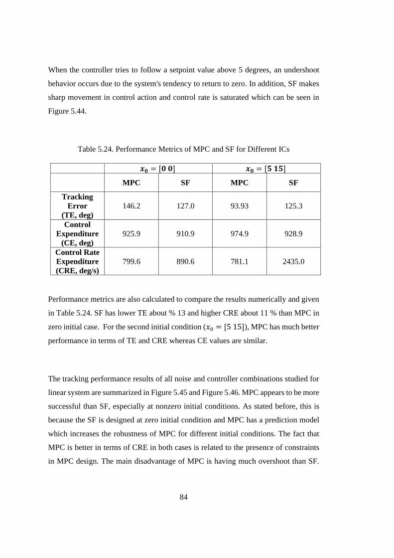
84
When the controller tries to follow a setpoint value above 5 degrees, an undershoot
behavior occurs due to the system's tendency to return to zero. In addition, SF makes
sharp movement in control action and control rate is saturated which can be seen in
Figure 5.44.
Table 5.24. Performance Metrics of MPC and SF for Different ICs
𝒙𝟎 = [𝟎 𝟎] 𝒙𝟎 = [𝟓 𝟏𝟓]
MPC SF MPC SF
Tracking
Error
(TE, deg)
146.2 127.0 93.93 125.3
Control
Expenditure
(CE, deg)
925.9 910.9 974.9 928.9
Control Rate
Expenditure
(CRE, deg/s)
799.6 890.6 781.1 2435.0
Performance metrics are also calculated to compare the results numerically and given
in Table 5.24. SF has lower TE about % 13 and higher CRE about 11 % than MPC in
zero initial case. For the second initial condition (𝑥0 = [5 15]), MPC has much better
performance in terms of TE and CRE whereas CE values are similar.
The tracking performance results of all noise and controller combinations studied for
linear system are summarized in Figure 5.45 and Figure 5.46. MPC appears to be more
successful than SF, especially at nonzero initial conditions. As stated before, this is
because the SF is designed at zero initial condition and MPC has a prediction model
which increases the robustness of MPC for different initial conditions. The fact that
MPC is better in terms of CRE in both cases is related to the presence of constraints
in MPC design. The main disadvantage of MPC is having much overshoot than SF.
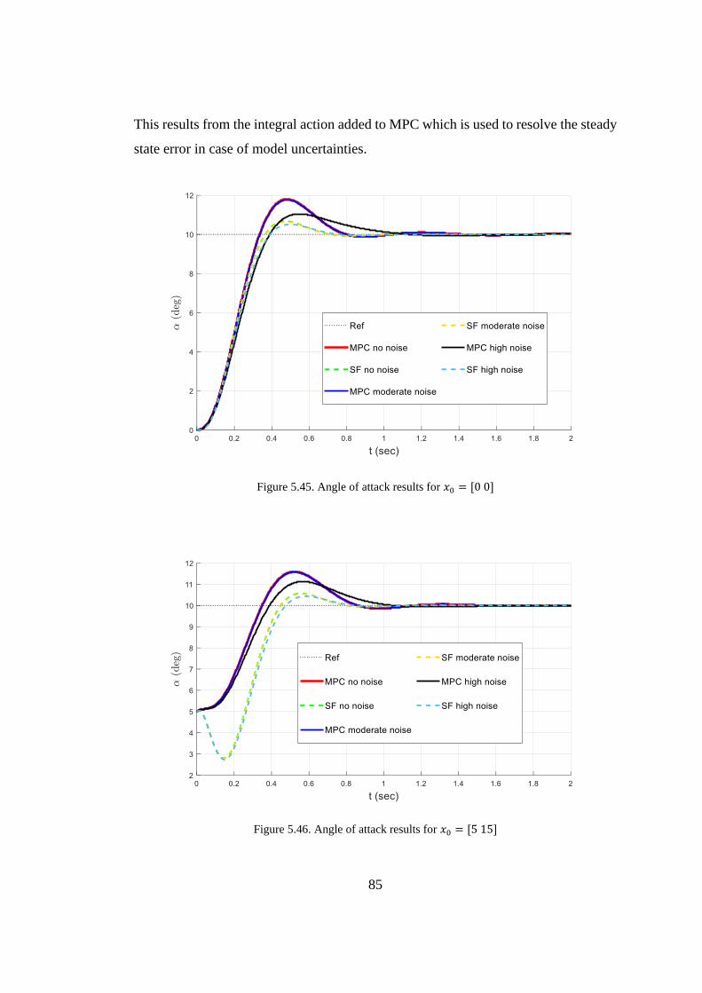
85
This results from the integral action added to MPC which is used to resolve the steady
state error in case of model uncertainties.
Figure 5.45. Angle of attack results for 𝑥0 = [0 0]
Figure 5.46. Angle of attack results for 𝑥0 = [5 15]

86
5.2.2. Control Performance Comparison for Non-Linear Missile Model
In this section, 3 control methods that is non-linear MPC, linear MPC and State
Feedback will be compared. In all methods, nonlinear system model given by Eqn.
(5-6) is used as true system model. The description of the methods is as follows.
1. Non-liner MPC (NMPC)
True system is controlled by MPC using the non-linear system model
discovered by SINDY.
2. Linear MPC (MPC)
True system is controlled by the MPC using the linearized system model that
is obtained using non-linear SINDY model.
3. State Feedback (SF)
True system is controlled by the state feedback using the linearized system
model that is obtained using non-linear SINDY model.
With this comparison, the performance of MPC and SF in the control of a nonlinear
system will be examined. In addition, the performances of using linear and nonlinear
prediction models in MPC will be analyzed. The true model and the previously
discovered models for clean and noisy measurements are given in Table 5.25.

87
Table 5.25. Discovered models using SINDY
True
model
Model-4
(Clean
Measurement)
Model-5
(Moderate
Noise)
Model-6
(High Noise)
�̇�𝟏
𝒙𝟏 -0.4382 -0.4495 -0.4454 -0.3981
𝒙𝟐 0.5392 0.5392 0.5368 0.5085
𝒖 -0.0243 0 0 0
𝒙𝟏𝟐 -0.2 -0.190 0 0
𝒙𝟏𝟑 4.5 4.927 5.7781 5.4889
𝒙𝟏𝟐𝒙𝟐 -1.2 -1.197 -1.1508 -0.9221
𝒙𝟏𝟐𝒖 100 98.77 95.9496 91.9266
�̇�𝟐
𝒙𝟏 -122.5085 -122.5085 -122.9884 -119.7355
𝒙𝟐 -1.0823 -1.0823 -1.0666 -0.9822
𝒖 102.7949 102.7949 102.5359 99.3816
𝒙𝟏𝟐 -120 -120.0000 -117.9593 110.1007
𝒙𝟏𝟑 -30 -30.0000 0 0
𝒙𝟐𝒖𝟐 20 20.0000 20.0004 0
MPC and State Feedback (SF) design parameters are given in Table 5.26 and Table
5.27 respectively.
Table 5.26. MPC design parameters for linear system
MPC Design
Parameters Values
Sample Time (Ts) 0.025
Prediction Horizon (Hp) 35
Control Horizon (Hm) 10
Output Weight (Q) 1.0
Input Rate Weight (R) 2.0
Input Constraints [-15, 15] deg
Input Rate Constraints [-250, 250] deg/s
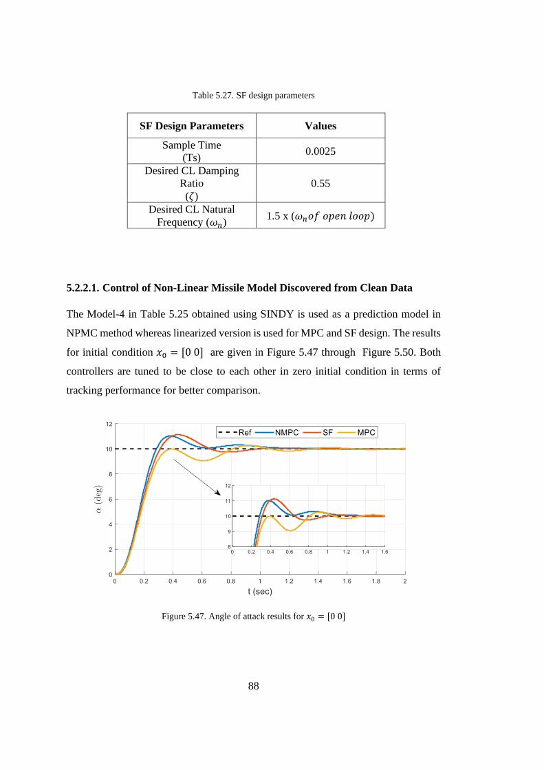
88
Table 5.27. SF design parameters
SF Design Parameters Values
Sample Time
(Ts) 0.0025
Desired CL Damping
Ratio
(𝜁)
0.55
Desired CL Natural
Frequency (𝜔𝑛) 1.5 x (𝜔𝑛𝑜𝑓 𝑜𝑝𝑒𝑛 𝑙𝑜𝑜𝑝)
5.2.2.1. Control of Non-Linear Missile Model Discovered from Clean Data
The Model-4 in Table 5.25 obtained using SINDY is used as a prediction model in
NPMC method whereas linearized version is used for MPC and SF design. The results
for initial condition 𝑥0 = [0 0] are given in Figure 5.47 through Figure 5.50. Both
controllers are tuned to be close to each other in zero initial condition in terms of
tracking performance for better comparison.
Figure 5.47. Angle of attack results for 𝑥0 = [0 0]
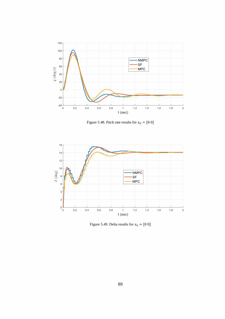
89
Figure 5.48. Pitch rate results for 𝑥0 = [0 0]
Figure 5.49. Delta results for 𝑥0 = [0 0]
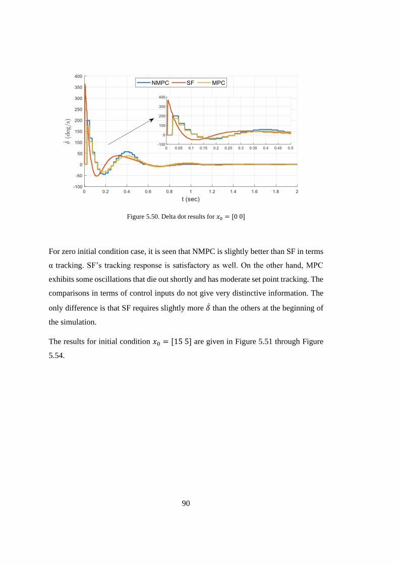
90
Figure 5.50. Delta dot results for 𝑥0 = [0 0]
For zero initial condition case, it is seen that NMPC is slightly better than SF in terms
α tracking. SF’s tracking response is satisfactory as well. On the other hand, MPC
exhibits some oscillations that die out shortly and has moderate set point tracking. The
comparisons in terms of control inputs do not give very distinctive information. The
only difference is that SF requires slightly more �̇� than the others at the beginning of
the simulation.
The results for initial condition 𝑥0 = [15 5] are given in Figure 5.51 through Figure
5.54.
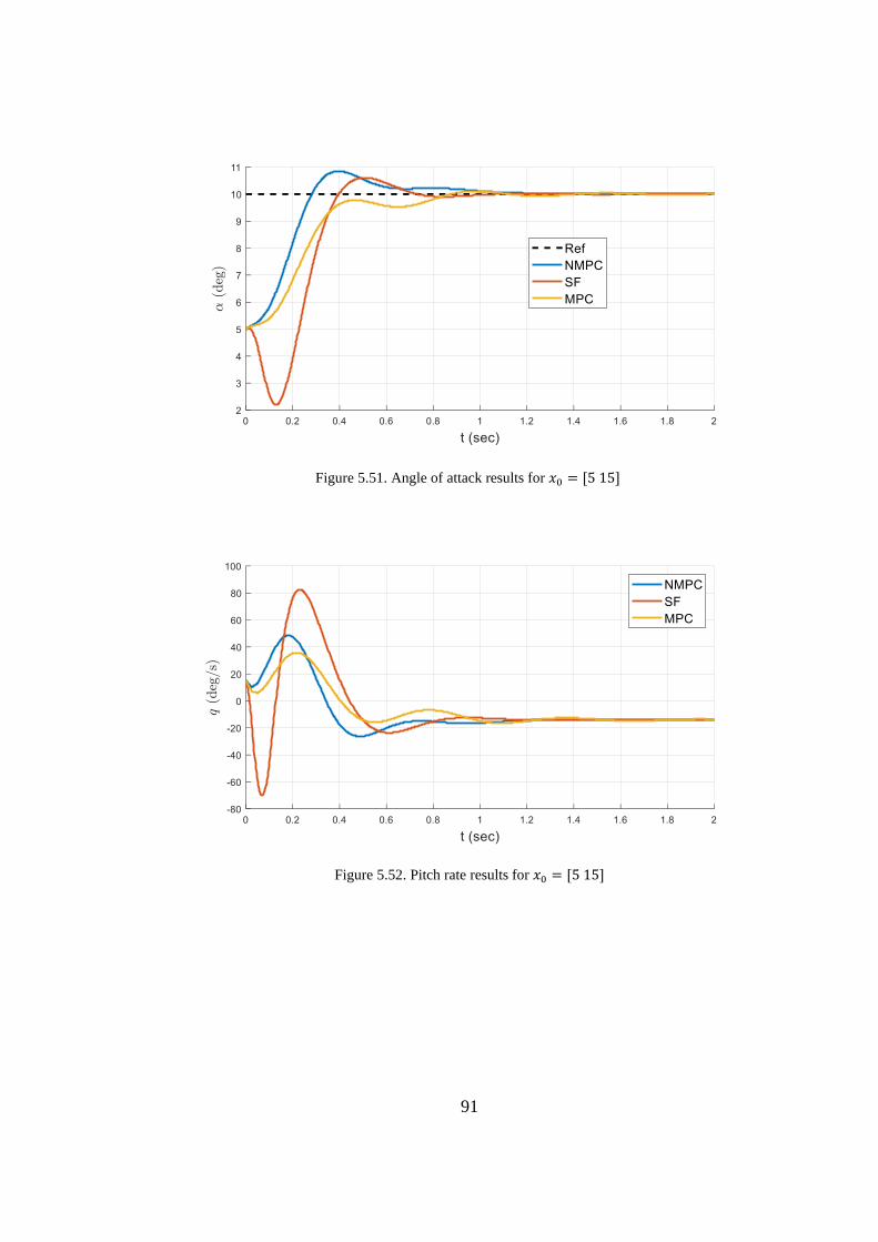
91
Figure 5.51. Angle of attack results for 𝑥0 = [5 15]
Figure 5.52. Pitch rate results for 𝑥0 = [5 15]
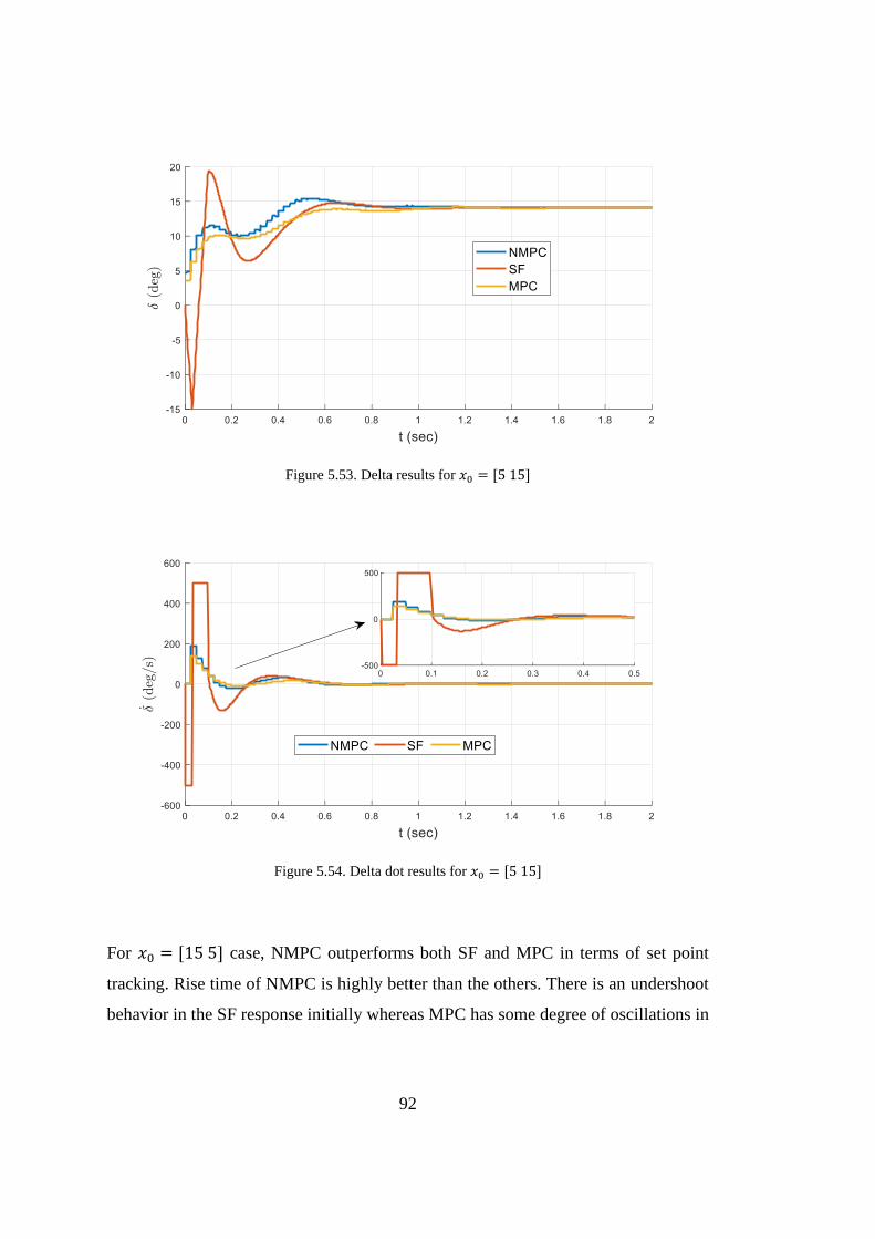
92
Figure 5.53. Delta results for 𝑥0 = [5 15]
Figure 5.54. Delta dot results for 𝑥0 = [5 15]
For 𝑥0 = [15 5] case, NMPC outperforms both SF and MPC in terms of set point
tracking. Rise time of NMPC is highly better than the others. There is an undershoot
behavior in the SF response initially whereas MPC has some degree of oscillations in
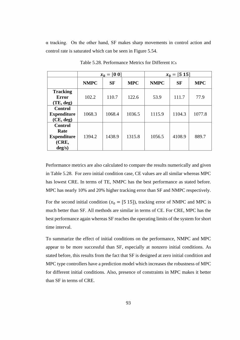
93
α tracking. On the other hand, SF makes sharp movements in control action and
control rate is saturated which can be seen in Figure 5.54.
Table 5.28. Performance Metrics for Different ICs
𝒙𝟎 = [𝟎 𝟎] 𝒙𝟎 = [𝟓 𝟏𝟓]
NMPC SF MPC NMPC SF MPC
Tracking
Error
(TE, deg)
102.2 110.7 122.6 53.9 111.7 77.9
Control
Expenditure
(CE, deg)
1068.3 1068.4 1036.5 1115.9 1104.3 1077.8
Control
Rate
Expenditure
(CRE,
deg/s)
1394.2 1438.9 1315.8 1056.5 4108.9 889.7
Performance metrics are also calculated to compare the results numerically and given
in Table 5.28. For zero initial condition case, CE values are all similar whereas MPC
has lowest CRE. In terms of TE, NMPC has the best performance as stated before.
MPC has nearly 10% and 20% higher tracking error than SF and NMPC respectively.
For the second initial condition (𝑥0 = [5 15]), tracking error of NMPC and MPC is
much better than SF. All methods are similar in terms of CE. For CRE, MPC has the
best performance again whereas SF reaches the operating limits of the system for short
time interval.
To summarize the effect of initial conditions on the performance, NMPC and MPC
appear to be more successful than SF, especially at nonzero initial conditions. As
stated before, this results from the fact that SF is designed at zero initial condition and
MPC type controllers have a prediction model which increases the robustness of MPC
for different initial conditions. Also, presence of constraints in MPC makes it better
than SF in terms of CRE.
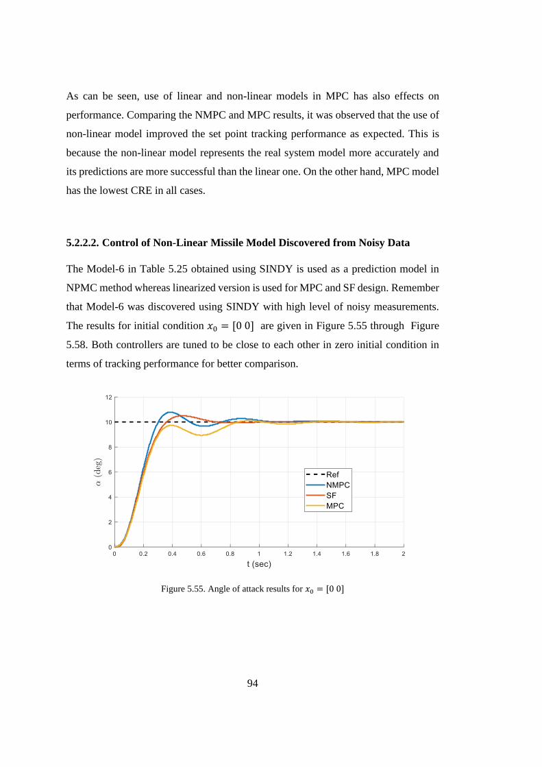
94
As can be seen, use of linear and non-linear models in MPC has also effects on
performance. Comparing the NMPC and MPC results, it was observed that the use of
non-linear model improved the set point tracking performance as expected. This is
because the non-linear model represents the real system model more accurately and
its predictions are more successful than the linear one. On the other hand, MPC model
has the lowest CRE in all cases.
5.2.2.2. Control of Non-Linear Missile Model Discovered from Noisy Data
The Model-6 in Table 5.25 obtained using SINDY is used as a prediction model in
NPMC method whereas linearized version is used for MPC and SF design. Remember
that Model-6 was discovered using SINDY with high level of noisy measurements.
The results for initial condition 𝑥0 = [0 0] are given in Figure 5.55 through Figure
5.58. Both controllers are tuned to be close to each other in zero initial condition in
terms of tracking performance for better comparison.
Figure 5.55. Angle of attack results for 𝑥0 = [0 0]
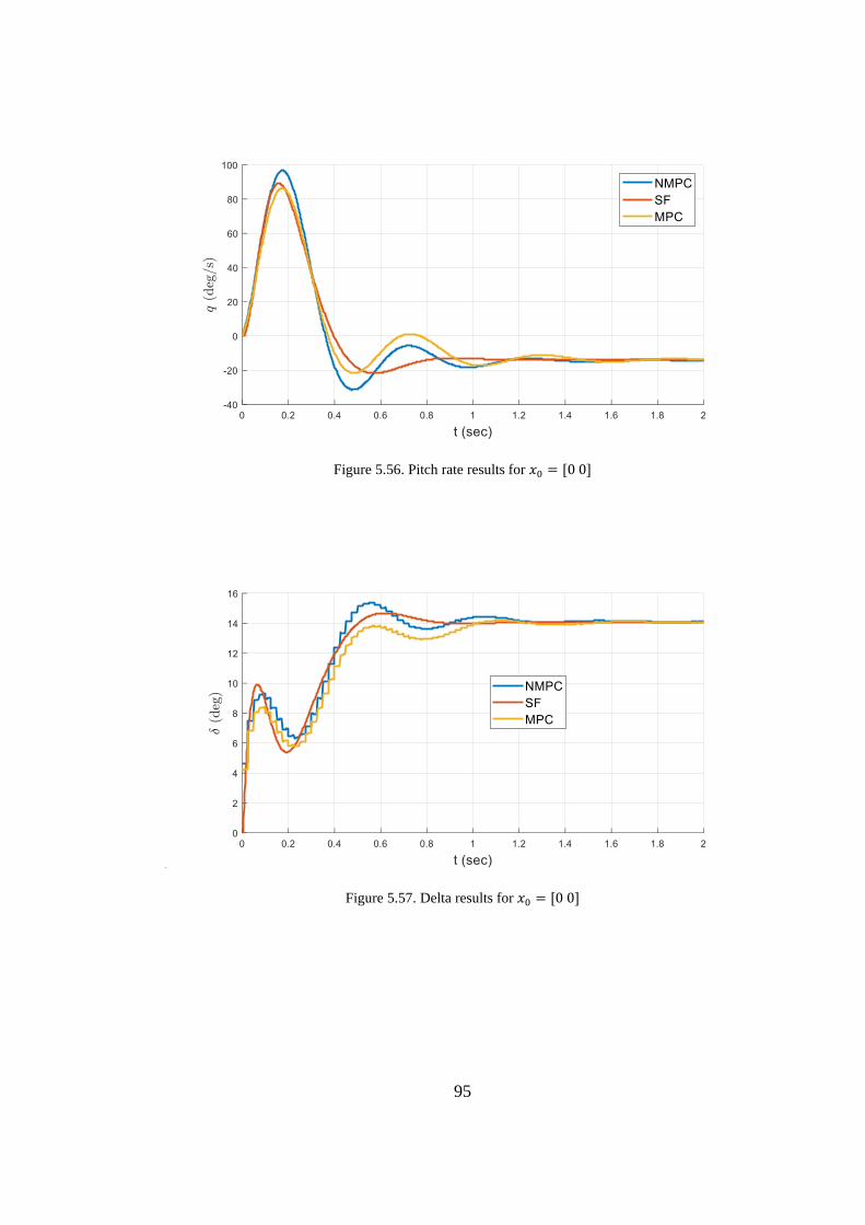
95
Figure 5.56. Pitch rate results for 𝑥0 = [0 0]
Figure 5.57. Delta results for 𝑥0 = [0 0]
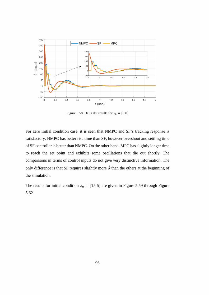
96
Figure 5.58. Delta dot results for 𝑥0 = [0 0]
For zero initial condition case, it is seen that NMPC and SF’s tracking response is
satisfactory. NMPC has better rise time than SF, however overshoot and settling time
of SF controller is better than NMPC. On the other hand, MPC has slightly longer time
to reach the set point and exhibits some oscillations that die out shortly. The
comparisons in terms of control inputs do not give very distinctive information. The
only difference is that SF requires slightly more �̇� than the others at the beginning of
the simulation.
The results for initial condition 𝑥0 = [15 5] are given in Figure 5.59 through Figure
5.62
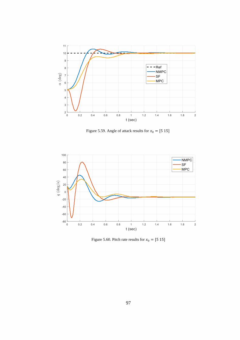
97
Figure 5.59. Angle of attack results for 𝑥0 = [5 15]
Figure 5.60. Pitch rate results for 𝑥0 = [5 15]
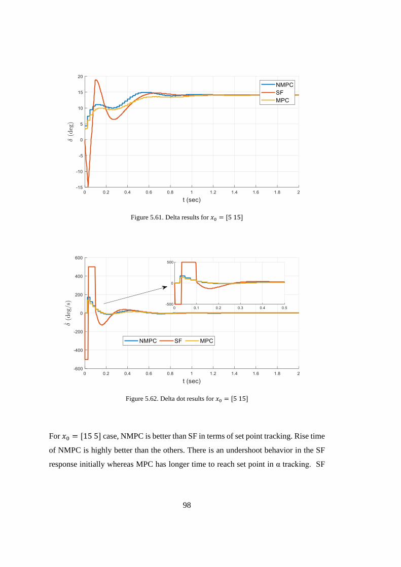
98
Figure 5.61. Delta results for 𝑥0 = [5 15]
Figure 5.62. Delta dot results for 𝑥0 = [5 15]
For 𝑥0 = [15 5] case, NMPC is better than SF in terms of set point tracking. Rise time
of NMPC is highly better than the others. There is an undershoot behavior in the SF
response initially whereas MPC has longer time to reach set point in α tracking. SF
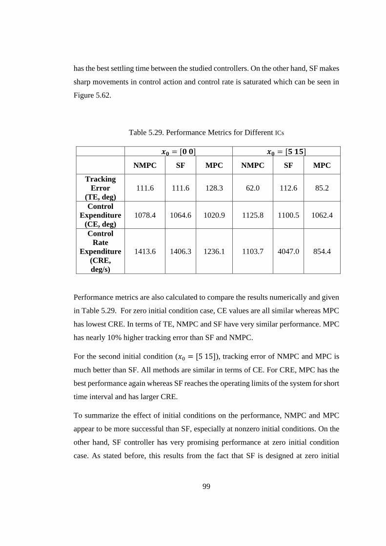
99
has the best settling time between the studied controllers. On the other hand, SF makes
sharp movements in control action and control rate is saturated which can be seen in
Figure 5.62.
Table 5.29. Performance Metrics for Different ICs
𝒙𝟎 = [𝟎 𝟎] 𝒙𝟎 = [𝟓 𝟏𝟓]
NMPC SF MPC NMPC SF MPC
Tracking
Error
(TE, deg)
111.6 111.6 128.3 62.0 112.6 85.2
Control
Expenditure
(CE, deg)
1078.4 1064.6 1020.9 1125.8 1100.5 1062.4
Control
Rate
Expenditure
(CRE,
deg/s)
1413.6 1406.3 1236.1 1103.7 4047.0 854.4
Performance metrics are also calculated to compare the results numerically and given
in Table 5.29. For zero initial condition case, CE values are all similar whereas MPC
has lowest CRE. In terms of TE, NMPC and SF have very similar performance. MPC
has nearly 10% higher tracking error than SF and NMPC.
For the second initial condition (𝑥0 = [5 15]), tracking error of NMPC and MPC is
much better than SF. All methods are similar in terms of CE. For CRE, MPC has the
best performance again whereas SF reaches the operating limits of the system for short
time interval and has larger CRE.
To summarize the effect of initial conditions on the performance, NMPC and MPC
appear to be more successful than SF, especially at nonzero initial conditions. On the
other hand, SF controller has very promising performance at zero initial condition
case. As stated before, this results from the fact that SF is designed at zero initial

100
condition and MPC type controllers have a prediction model which increases the
robustness of MPC for different initial conditions. Also, presence of constraints in
MPC makes it better than SF in terms of CRE.
As can be seen, use of linear and non-linear models in MPC has also effects on
performance. Similar to the case of clean measurements at previous section,
comparing the NMPC and MPC results show that the use of non-linear model
improved the set point tracking performance as expected. This is because the non-
linear model represents the real system model more accurately and its predictions are
more successful than the linear one. On the other hand, MPC model has the lowest
CRE in all cases.

101
CHAPTER 6
6. DISCUSSION
The proposed SINDY-SAIC algorithm determined the important dynamics of the
longitudinal missile system accurately for clean, moderate and high level of noise
cases. In case of clean measurement of states, SINDY-SAIC could find the
coefficients of the true model with great accuracy whereas for noisy data, all the
important dynamics of the system was captured with at most 10% error in the
coefficients.
Calculation of state derivatives using sliding window approach significantly increased
the robustness of SINDY-SAIC to noise.
In addition, the proposed algorithm eliminated the need for threshold parameters
tuning and presence of AIC model selection enables to select the most sparse solutions
among many others.
Furthermore, MPC and state feedback controllers were designed using discovered
models. All controller’s performances such as tracking, control expenditure and
control rate expenditure were compared. For linear missile system, MPC appears to
be more successful than SF, especially at nonzero initial conditions. This is because
MPC uses the prediction model to overcome initial condition changes. Also, MPC
requires less control rate due to the presence of constraints inherently.
For non-linear missile system, NMPC and SF performed similarly for zero initial
condition case whereas MPC has slightly longer time to reach the set point and
exhibits some oscillations. In non-zero initial condition, NMPC is better than SF.
MPC and SF are similar in terms of set point tracking. All controllers tracked the set
point successfully and exhibit stable behavior under uncertainties. Therefore, an
appropriate controller can be selected according to the controller requirements.

102
This study motivates several future investigations and extensions such as:
• Measurement data obtained from real flight tests could be used to check the
robustness of the SINDY-SAIC algorithm.
• Hardware implementation of the algorithm and the controllers could be done
on cost effective platforms such as CPUs, GPUs, or FPGAs.
• It is possible to use SINDY-SAIC online since its convergence rate is very
high. Especially with linear SINDY, an approximate linear model could be
built quickly, and then more exact nonlinear model could be estimated in
parallel with increasing amount of data online.
• In addition, if there are known terms, functions, and constraints in the dynamic
model of the system, this knowledge could also be included in the SINDY-
SAIC algorithm to increase accuracy and speed.
• The required full-state measurements were assumed to be available in this
study. Instead, state estimation and mapping techniques could be used to
convert measurements to appropriate basis for better generalization.
• Nonlinear integral action was added to MPC to avoid steady state errors in case
of model uncertainties. This resulted in slight overshoot in the response.
Different nonlinear functions for integral action could be further analyzed.
103
REFERENCES
[1] A. Punjani and P. Abbeel, “Deep learning helicopter dynamics models,” in
IEEE International Conference on Robotics and Automation (ICRA), 2015, vol.
20, pp. 3223–3230.
[2] Y. Kang, S. Chen, X. Wang, and Y. Cao, “Deep Convolutional Identifier for
Dynamic Modeling and Adaptive Control of Unmanned Helicopter,” in IEEE
Transactions on Neural Networks and Learning Systems, 2019, vol. 30, no. 2,
pp. 524–538.
[3] D. Rolnick and M. Tegmark, “The power of deeper networks for expressing
natural functions,” 6th Int. Conf. Learn. Represent. ICLR, pp. 1–14, 2018.
[4] H. W. Lin, M. Tegmark, and D. Rolnick, “Why does deep and cheap learning
work so well?,” J. Stat. Phys., vol. 168, no. 6, pp. 1223–1247, 2017.
[5] M. Raissi, P. Perdikaris, and G. E. Karniadakis, “Physics Informed Deep
Learning (Part II): Data-driven Discovery of Nonlinear Partial Differential
Equations,” no. Part II, pp. 1–19, 2017.
[6] E. Kilic, M. Dolen, A. B. Koku, H. Caliskan, and T. Balkan, “Accurate pressure
prediction of a servo-valve controlled hydraulic system,” Mechatronics, vol. 22
(7), pp. 997–1014, 2012.
[7] E. Kilic, M. Dolen, H. Caliskan, A. B. Koku, and T. Balkan, “Pressure
prediction on a variable-speed pump controlled hydraulic system using
structured recurrent neural networks,” Control Eng. Pract., vol. 26, pp. 51–71,
2014.
[8] B. O. Koopman, “Hamiltonian Systems and Transformations in Hilbert Space,”
Mathematics, vol. 17, pp. 315–318, 1931.
[9] M. Budišić, R. Mohr, and I. Mezić, “Applied Koopmanism,” Chaos, vol. 22,
no. 4, 2012.
[10] I. Mezić, “Spectral properties of dynamical systems, model reduction and
decompositions,” Nonlinear Dyn., vol. 41, no. 1–3, pp. 309–325, 2005.
[11] M. Korda and I. Mezić, “Linear predictors for nonlinear dynamical systems:
Koopman operator meets model predictive control,” Automatica, vol. 93, pp.
149–160, 2018.
[12] J. P. Boyd, “Chebyshev & Fourier Series,” Chebyshev Fourier Spectr. Methods,
pp. 19–60, 2000.
[13] H. Wendland, “Meshless Galerkin methods using radial basis functions,” Math.
Comput., vol. 68, no. 228, pp. 1521–1532, 1999.
[14] B. Lusch, J. N. Kutz, and S. L. Brunton, “Deep learning for universal linear
104
embeddings of nonlinear dynamics,” Nat. Commun., vol. 9, no. 1, 2018.
[15] M. Quade, M. Abel, J. Nathan Kutz, and S. L. Brunton, “Sparse identification
of nonlinear dynamics for rapid model recovery,” Chaos, vol. 28, no. 6, pp. 1–
10, 2018.
[16] S. L. Brunton, J. L. Proctor, and J. Nathan Kutz, “Supporting Information for:
Discovering governing equations from data: Sparse identification of nonlinear
dynamical systems,” Nat. Commun., vol. 8, no. 1, pp. 1–38, 2017.
[17] H. Schaeffer, “Learning partial differential equations via data discovery and
sparse optimization,” Proc. R. Soc. A Math. Phys. Eng. Sci., vol. 473, no. 2197,
2017.
[18] S. L. Brunton, J. L. Proctor, J. N. Kutz, and W. Bialek, “Discovering governing
equations from data by sparse identification of nonlinear dynamical systems,”
Proc. Natl. Acad. Sci. U. S. A., vol. 113, no. 15, pp. 3932–3937, 2016.
[19] K. Kaheman, J. N. Kutz, and S. L. Brunton, “SINDy-PI: A robust algorithm for
parallel implicit sparse identification of nonlinear dynamics: SINDy-PI,” Proc.
R. Soc. A Math. Phys. Eng. Sci., vol. 476, no. 2242, 2020.
[20] N. M. Mangan, S. L. Brunton, J. L. Proctor, and J. N. Kutz, “Inferring
Biological Networks by Sparse Identification of Nonlinear Dynamics,” IEEE
Trans. Mol. Biol. Multi-Scale Commun., vol. 2, no. 1, pp. 52–63, 2016.
[21] L. Boninsegna, F. Nüske, and C. Clementi, “Sparse learning of stochastic
dynamical equations,” J. Chem. Phys., vol. 148, no. 24, 2018.
[22] H. Akaike, “Information Theory and an Extension of the Maximum Likelihood
Principle,” 2nd Int. Symp. Inf. Theory, vol. 90, no. 29, pp. 267–281, 1973.
[23] H. Akaike, “A New Look at the Statistical Model Identification,” IEEE Trans.
Automat. Contr., vol. 19, no. 6, pp. 716–723, 1974.
[24] L. I. Rudin, S. Osher, and E. Fatemi, “Nonlinear total variation based noise
removal algorithms,” Phys. D, vol. 60, no. 1–4, pp. 259–268, 1992.
[25] S. L. Brunton and J. N. Kutz, Data Driven Science & Engineering - Machine
Learning, Dynamical Systems, and Control. Lauren Cowles,Cambridge, 2017.
[26] E. Kaiser, J. N. Kutz, and S. L. Brunton, “Sparse identification of nonlinear
dynamics for model predictive control in the low-data limit,” Proc. R. Soc. A
Math. Phys. Eng. Sci., vol. 474, no. 2219, 2018.
[27] H. Zhu, “On Information and Sufficiency,” Ann. Stat., pp. 1–5, 1997.
[28] S. Kullback, Information theory and statistics. Dover Publications, 1968.
[29] C. M. Hurvich and C. L. Tsai, “Regression and time series model selection in
105
small samples,” Biometrika, vol. 76, no. 2, pp. 297–307, 1989.
[30] J. M. Maciejowski, Predictive Control with Constraints. Prentice Hall, 2000.
[31] R. H. Bishop, Model Based Predictive Control-A Practical Approach. CRC
Press LLC, 2005.
[32] K. R. Muske and T. A. Badgwell, “Disturbance modeling for offset-free linear
model predictive control,” J. Process Control, vol. 12, no. 5, pp. 617–632,
2002.
[33] C. V Rao, S. J. Wright, and J. B. Rawlings, “Application of interior-point
methods to model predictive control,” vol. 99, no. 3, pp. 723–758, 1998.
[34] Y. Cao, “Nonlinear Model Predictive Control Using Automatic
Differentiation,” IFAC Proc. Vol., vol. 16, pp. 1037–1042, 2005.
[35] R. M. Howard, “Dynamics of Flight: Stability and Control; Third Edition,” J.
Guid. Control. Dyn., vol. 20, no. 4, pp. 839–840, 1997.
[36] K. Ogata, Modern Control Engineering, 4th ed., vol. 39, no. 12. Prentice Hall,
New Jersey, 2002.