Data-driven patient motion compensation in cardiac positron

emission tomography

by

Spencer Thomas Manwell

A thesis submitted to the Faculty of Graduate and Postdoctoral Affairs in partial

fulfillment of the requirements for the degree of

Doctor of Philosophy

in

Physics

Specialization in Medical Physics

Ottawa-Carleton Institute for Physics

Department of Physics

Carleton University

Ottawa, Ontario

© 2020, Spencer Thomas Manwell

i

Abstract

Positron emission tomography (PET) is a molecular imaging modality that has been

demonstrated to be a powerful, non-invasive, tool for the assessment and diagnosis of

cardiac pathologies like coronary artery disease. The accuracy of these clinical

examinations for detecting and prognosticating disease can be marred in cases where

patient motion is severe. Clinical use of motion tracking/compensation tools, however, is

relatively uncommon partly due to the increases in complexity and time of patient setup

prior to imaging. The purpose of the work described here was to develop and evaluate new

methods of patient motion detection and compensation in the context of cardiac PET

imaging studies that are less complex than standard commercial options in the hope of

reducing barriers to clinical adoption.

The proposed methods are based on measuring and tracking the motion of a low-activity

radioactive marker placed on patients using the positron emission tracking (PeTrack)

algorithm. Motion information was employed to compensate and/or correct for either

respiratory or whole-body patient motion.

The performance of PeTrack for respiratory tracking and motion compensation was

evaluated in a clinical population in comparison with a commonly used commercial optical

tracking device. Within a practical comparison framework PeTrack was shown to perform

comparably to the commercial system. From this comparison shortcomings of both

PeTrack and the commercial system were identified; knowledge of the former can inform

future development and improvement.

A method for whole-body patient motion correction (WBMC) in static cardiac perfusion

studies using PeTrack was developed. Motion corrected images demonstrated significantly

ii

less blurring of the myocardial walls and improved contrast. Relative perfusion

measurements among the clinical data sets were not significantly affected although the

extent of patient motion was limited.

The WBMC algorithm was extended for dynamic acquisitions used for quantification of

myocardial blood flow. Motion detection and estimation with PeTrack was compared to

that of another data-driven motion tracking algorithm within a clinical population. Body

motion estimation with PeTrack was more robust than the alternative method. Motion

correction using PeTrack demonstrated improvement among various quality indicators of

the kinetic modelling used to estimate blood flow.

iii

Acknowledgements

There were many who contributed to this work either directly and indirectly and it is

difficult to overstate the importance of each. I will do my best to acknowledge these

individuals and organizations here, but I am sure that I will not do so sufficiently. I had

the unique experience of being co-supervised by three people. In no particular order, I

would like to express my sincere gratitude to Dr. Ran Klein, Dr. Robert deKemp, and Dr.

Tong Xu for investing their time and resources into my training during my doctoral

studies. Each of these individuals have unique strengths and I am confident that I was

able to absorb some of these from each of them. Ran Klein is a spectacular engineer and

he never missed an opportunity to impress upon me the value of good design and the

importance of automation. Together these concepts lead to the development of things that

are, hopefully, as easy as possible to use and to share with others. Whether I was writing

computer code, or imagining an experiment, I tried in earnest to incorporate these

notions. Robert deKemp showed me the importance of understanding the data within a

study and how important findings can be made that are outside of the principle research

questions and are often found in the fringe cases of your study. Unless one closely

examines all the data points and asks questions regarding their relationships, information

will undoubtedly go unnoticed. Tong Xu is a very talented physicist and regularly

demonstrated how important it was to consider questions and interpret results from first

principles - in the end everything is explainable and one should seek to do so with respect

to basic concepts that are well founded. Thank you, all of you, for sharing your gifts with

me.

iv

While less directly involved in my work, the people with whom I spent most of my

office/study time with also are deserving of my thanks. My peers, my colleagues, my

friends, provided useful suggestions, necessary distractions, and companionship beyond

the boundaries of study. So, Sarah Cuddy-Walsh, Owen Clarkin, Jennifer Renaud, Hanif

Juma, Odai Salman, Chad Hunter, Zahra Ashoori, Robert Miner, Eric Christiansen, Chris

Dydula, Ming Liu, Alexandra Bourguoin, Marc Chamberland, Martin Martinov, Nick

Majtenyi, Iymad Mansour, and Nathan Murtha, thank you for your friendship, your help,

and your encouragement.

Several other staff at researchers at University of Ottawa Heart Institute and Carleton

University were also very helpful and supportive during my studies. Dr. R. Glenn Wells,

thank you for helpful comments on several presentations that I delivered and also for

letting me borrow one your text books – at the time of writing this I still have yet to

return it to you. Ms. May Aung, Ms Kimberly Gardner, and Ms. Azmina Merani, are

nuclear medicine technologists at UOHI, all of whom were incredibly helpful, friendly,

and patient with me when I needed to use the PET scanner console. Thank you all very

much for your help, getting to know each of you was my privilege. Ms. Alison Conley,

and Ms. Ann Nguyen of UOHI Research Services helped me on many occasions with

travel/funding applications, thank you both. Ms. Eva Lacelle and Ms. Temi Gouti both

held the incredibly important position of Graduate Student Administrator with the

Carleton Physics Department. These two individuals acted as the buffer between anxious

graduate students (myself, at least) and the confusing world of university bureaucracy,

most importantly both of you helped make sure that I received my funding; thank you

very, very much. Several Carleton Physics faculty members involved with advising

v

graduate students also deserve my thanks; Dr. Heather Logan, Dr. Paul Johns, Dr. Kevin

Graham, thank you all very much for your dedication to graduate student success in our

department.

I would also like to acknowledge the research funding agencies who not only supported

my work, but who help facilitate the provision of financial support for graduate students

who, in many cases, sacrifice higher pay in the workforce to pursue their passions and

help drive Canadian research. The Government of Ontario, the National Sciences and

Engineering Research Council of Canada, the Canadian Institutes of Health research, the

Carleton University Faculty of Graduate and Post-Doctoral Affairs, the Ottawa Heart

Institute Research Corporation, and the IEEE Nuclear and Plasma Sciences Society, have

all contributed to varying degrees to my research and travel funding.

To my parents, thank you for your love and support not only during this degree but

during my whole life. I am sure that you have shaped the curiosities I now have about the

world which have certainly guide me to path on which I now find myself. You have

helped me, and my own young family, with so many things that allowed me to continue

to focus on my research – I only hope that I can someday return the kindness.

To my wife and partner, Robyn, it is impossible to express in words the appreciation,

admiration, and respect that I have for you. You supported us and made the life that we

have built together possible while I underwent this half-decade pursuit. Beyond your love

and encouragement, you have given me (us) two beautiful sons who at the current ages of

3 years and 2 weeks, have completely reshaped my life, values, and purpose. I will never

fail to recognize and appreciate the personal sacrifices that you have made so that we can

have the life we’d hoped for while I spent this time chasing a dream. Thank you.

vi

To my sons,

Henry and Oliver.

“I would not be one of those who will foolishly drive a nail into mere

lath and plastering; such a deed would keep me awake nights. Give me

a hammer, and let me feel for the furring. Do not depend on the putty.

Drive a nail home and clinch it so faithfully that you can wake up in the

night and think of your work with satisfaction -- a work at which you

would not be ashamed…”

This passage, from Henry David Thoreau’s Walden, really struck me when I first came

upon it. What I took from it was this; whatever it is that you choose to do, do it with all

your heart and to the best of your ability.

vii

Contributions

The work described in this thesis represent a detailed summary of my research

activities during my doctoral studies. All work was performed under the co-supervision

of (in no particular order) Dr. Ran Klein, Dr. Robert deKemp, and Dr. Tong Xu, each of

whom provided guidance to me while designing studies, analyzing data, interpreting

results and preparing materials for dissemination during presentations or manuscripts.

This work represents the most comprehensive application of the Positron Emission

Tracking (PeTrack) algorithm to the clinical setting for the purpose of patient motion

compensation in cardiac PET imaging. It also represents the first application of PeTrack

for to whole-body motion correction in dynamic cardiac PET studies, as well as to

cardiac PET studies that used 13N-Ammonia as the radiotracer.

All image reconstructions described in this thesis were performed using research

software developed by the manufacturer (GE Healthcare) of the PET scanners at the

University of Ottawa Heart Institute. I developed various additions to this package that

were necessary to generate gated images from list-mode data. I created utilities that gated

dead time and single-event count rate data from the list-mode data files, incorporated

respiratory and body-motion triggers from algorithms developed and/or implemented,

incorporated spatial transformations to extend the software to permit motion

compensation, and extended the DICOM file writing utilities to include fields needed for

image viewers to correctly interpret 4D image data sets. Lastly, I extended the software to

perform post-reconstruction image registration for estimating patient body motion. Prior

to my use of it, the reconstruction software was significantly refactored for ease of use by

Dr. Chad Hunter.

viii

I drafted the study protocol which was submitted to the UOHI Ethics Board to attain

retrospective access to the clinical data sets described in this thesis. The protocol was

additionally reviewed by Dr. Robert deKemp and Ms. Linda Garrard. The protocol was

modified by myself and reviewed by Dr. Tong Xu for submission to the Carleton

University Ethics Board to attain permission to conduct my research involving human

patient data. I collected all clinical data sets used within this thesis following the de-

identification and archival measures described in the REB-approved study protocol.

The PeTrack ADROI code used extensively throughout my work was developed by Dr.

Marc Chamberland and Dr. Tong Xu. I contributed to this software package by including

methods for producing respiratory and body-motion triggers from PeTrack motion traces.

I implemented a respiratory trigger detection algorithm had been previously published

(described in Chapter 3) and created two methods for body-motion detection (described

in Chapter 4 and Chapter 5). I included methods for stochastically sampling list-mode

data files to manipulate image noise (described in Chapter 3). Based on the PeTrack

ADROI code, I also implemented a previously published data-driven motion tracking

algorithm known as the Centroid-of-Distribution (COD) method which modifications that

allows the user to limit the list-mode events that are used during tracking (described in

Chapter 5). I developed an automated tool to measure myocardial wall thicknesses from

PET images as described in Chapter 3 and Appendix A. I also proposed a respiratory

trigger quality control framework based on previous work aimed at cardiac (ECG)

triggering.

ix

I designed the phantom experiment described in Chapter 4 and fabricated a translatable

table with which rigid patient motion was simulated. The experiment was performed by

Dr. Robert deKemp, Dr. Tong Xu, Dr. Ran Klein and myself.

I disseminated my research through peer-review publication, conference proceedings,

and oral and poster presentations. These are listed below.

Peer-reviewed papers:

1. Spencer Manwell, Ran Klein, Tong Xu, Robert deKemp, “Clinical comparison of

the Positron Emission Tracking (PeTrack) algorithm with the Real-Time Position

Management System for respiratory gating in cardiac positron emission

tomography”, Medical Physics 2020; 47(4): 1713-1726, DOI:

10.1002/mp.14052.i,151

Conference proceedings:

1. S. Manwell, R. Klein, R. deKemp, T. Xu, “Whole-body motion correction 13N-

ammonia myocardial perfusion imaging using positron emission tracking”, 2019

IEEE Nuclear Science Symposium and Medical Imaging Conference (NSS/MIC)

Record, Manchester UK, November 2019, pp 1-5, DOI:

10.1109/NSS/MIC42101.2019.9059704ii,168

2. S. Manwell, R. Klein, R. deKemp, T. Xu, “Whole-body motion correction in

cardiac PET/CT using Positron Emission Tracking: A phantom validation study”,

2018 IEEE Nuclear Science Symposium and Medical Imaging Conference

i This publication was modified for inclusion in this thesis and comprises the content of Chapter 3. ii The poster for this abstract was shown again at the Carleton University Life Sciences Day, Ottawa,

ON, May 2018 and awarded 1st place among graduate student posters.

x

(NSS/MIC) Record, Sydney, AU, October 2018, pp 1-3, DOI:

10.1109/NSSMIC.2018.8824715.iii,167

3. S. Manwell, M. Chamberland, R. Klein, T. Xu, R. deKemp, “Evaluation of the

clinical efficacy of the PeTrack motion tracking system for respiratory gating in

cardiac PET imaging”, Proc. SPIE 10132, Medical Imaging 2017: Physics of

Medical Imaging, 1013251 (9 March 2017), Orlando, FL, 10.1117/12.2255544.157

Conference abstracts:

1. Spencer Manwell, Ran Klein, Tong Xu, and Robert deKemp, “‘Bad-Breath’

Rejection: quality control metrics for respiratory gating in PET/CT.”, Society of

Nuclear Medicine and Molecular Imaging (SNMMI) Annual Meeting, Anaheim,

CA, June 2019. Published in J. Nucl. Med. May 1, 2019, vol. 60 no. supplement 1,

1366.

2. Spencer Manwell, Ran Klein, Tong Xu, and Robert deKemp, “Data-driven

respiratory gating in cardiac PET/CT using the Positron Emission Tracking

Algorithm”, Society of Nuclear Medicine and Molecular Imaging (SNMMI)

Annual Meeting, Philadelphia, PA, June 2018. Published in J. Nucl. Med. May 1,

2018, vol. 59 no. supplement 1, 16.

3. Spencer Manwell, Ran Klein, Robert deKemp, Tong Xu, “Patient motion

management using the positron emission tracking (PeTrack) algorithm in cardiac

iii This abstract was reformatted abstract as an oral presentation and presented at The Ottawa Hospital

Department of Medicine Research Day, Ottawa, ON, May 2019, and awarded Best Graduate Student

Scientific Presentation. The original poster was also presented at the Carleton University Life Sciences

Day, Ottawa, ON, May 2017 and awarded 2nd place among graduate student posters.

xi

PET without time-of-flight”, Canadian Organization of Medical Physicists 63rd

Annual Scientific Meeting, Ottawa, Canada, July 2017.

xii

Table of Contents

Abstract ........................................................................................................................... i

Acknowledgements ....................................................................................................... iii

Contributions ............................................................................................................... vii

Table of Contents ......................................................................................................... xii

List of Tables .............................................................................................................. xvii

List of Illustrations ..................................................................................................... xix

List of Acronyms ...................................................................................................... xxxv

Chapter 1 Introduction ........................................................................................... 1

1.1 Physics of Nuclear Medicine .......................................................................................... 2

1.1.1 Nuclear Structure, Stability and Radioactive Decay .............................................. 2

1.1.2 Interactions of Radiation with Matter .................................................................... 8

1.2 Positron Emission Tomography ................................................................................... 13

1.2.1 Photon Detection with Scintillators ..................................................................... 14

1.2.2 PET System Design and Performance ................................................................. 20

1.2.2.1 Spatial Resolution ....................................................................................... 24

1.2.2.2 Energy Resolution ....................................................................................... 25

1.2.2.3 Timing Resolution ....................................................................................... 25

1.2.2.4 Dead Time and Count Rate Performance .................................................... 25

1.2.2.5 Sensitivity .................................................................................................... 27

1.2.2.6 Performance Characteristics of GE Discovery 690 PET/CT System .......... 28

1.2.3 Data Correction for Quantitative PET ................................................................. 29

1.2.3.1 Normalization correction ............................................................................ 30

1.2.3.2 Random Coincidence Correction ................................................................ 30

1.2.3.3 Dead Time Correction ................................................................................. 31

xiii

1.2.3.4 Attenuation Correction ................................................................................ 31

1.2.3.5 Scatter Correction........................................................................................ 33

1.2.4 Tomographic Image Reconstruction .................................................................... 35

1.3 Imaging the Heart with PET ......................................................................................... 40

1.3.1 Anatomy of the Heart and Electrocardiographic Signals ..................................... 40

1.3.2 Myocardial Perfusion Imaging with PET ............................................................ 45

1.3.3 Kinetic Tracer Modelling and Estimate of Absolute Myocardial Blood Flow .... 51

1.4 Thesis Summary ........................................................................................................... 57

Chapter 2 Patient Motion Tracking and Compensation ................................... 59

2.1 Patient Motions: Respiratory, Cardiac and Body ......................................................... 59

2.2 Motion Tracking ........................................................................................................... 63

2.2.1 Hardware-Based Tracking ................................................................................... 65

2.2.2 Data-Driven Tracking .......................................................................................... 68

2.3 Compensation and Correction ...................................................................................... 71

2.3.1 Breath-hold Techniques and Patient Immobilization .......................................... 71

2.3.2 Respiratory and Cardiac Gating ........................................................................... 73

2.3.3 Motion Correction................................................................................................ 76

2.4 Positron Emission Tracking (PeTrack) ......................................................................... 80

2.4.1 The Tracking Algorithm ...................................................................................... 80

2.4.2 Motivation for the Use of PeTrack in PET .......................................................... 85

Chapter 3 Respiratory Gating in Cardiac Perfusion PET ................................ 89

3.1 Motivation .................................................................................................................... 89

3.2 Methods ........................................................................................................................ 90

3.2.1 Respiratory-Gated Acquisition ............................................................................ 90

3.2.2 Patient Population ................................................................................................ 92

3.2.3 Respiratory-Signal Generation ............................................................................ 93

xiv

3.2.4 Respiratory-Gating and Image Reconstruction .................................................... 94

3.2.5 Measurements for Comparison ............................................................................ 95

3.2.6 Comparing Respiratory Signals and Triggers ...................................................... 96

3.2.7 Comparing Image-Based Measurements ............................................................. 98

3.2.8 Statistical Methods ............................................................................................. 101

3.3 Results ........................................................................................................................ 101

3.4 Discussion................................................................................................................... 109

3.4.1 Respiratory Signal and Trigger Measurements .................................................. 110

3.4.2 Quality Control .................................................................................................. 113

3.4.3 Image based motion estimates ........................................................................... 116

3.4.4 Considerations for PeTrack ............................................................................... 117

3.4.5 Clinical Use of PeTrack for Respiratory Gating ................................................ 119

3.5 Conclusion .................................................................................................................. 121

Chapter 4 Whole-Body Motion Correction in Myocardial Perfusion Imaging

with PET/CT ............................................................................................................. 122

4.1 Motivation .................................................................................................................. 122

4.2 Methods ...................................................................................................................... 123

4.2.1 Whole-Body Motion Correction Framework ..................................................... 123

4.2.2 Validation Using an Anthropomorphic Torso Phantom .................................... 127

4.2.3 Application to 13N-Ammonia Perfusion Studies ................................................ 128

4.2.4 Quantitative Measurements ............................................................................... 129

4.3 Results ........................................................................................................................ 133

4.3.1 Motion Tracking Validation .............................................................................. 133

4.3.2 LV Wall Thickness and Blood Pool Volume Comparison ................................ 137

4.3.3 Effects of Motion Correction on CNR ............................................................... 141

4.3.4 Relative Perfusion and Left-Ventricular Volumes ............................................ 144

xv

4.4 Discussion................................................................................................................... 144

4.5 Conclusions ................................................................................................................ 150

Chapter 5 Whole-Body Motion Correction for Absolute Blood Flow

Quantification ............................................................................................................. 151

5.1 Motivation .................................................................................................................. 151

5.2 Methods ...................................................................................................................... 152

5.2.1 Centroid of Distribution (COD) Motion Tracking ............................................. 152

5.2.2 Whole-Body Motion Detection ......................................................................... 155

5.2.3 Motion Estimation and Correction .................................................................... 158

5.2.4 Clinical Dataset .................................................................................................. 162

5.2.5 Verification of COD Tracking and Image Registration Methods ...................... 164

5.2.6 Absolute Blood Flow Quantification and Figures of Merit ............................... 166

5.3 Results ........................................................................................................................ 170

5.3.1 Verification of COD Tracking ........................................................................... 170

5.3.2 Verification of the Image Registration Method ................................................. 173

5.3.3 Evaluation of the Body-Motion Detection and Estimation Methods ................. 174

5.3.4 Sensitivity of Kinetic Modelling Quality Metrics to Motion ............................. 176

5.3.5 Patient Motion Assessment Among Severe Motion Cases ................................ 177

5.3.6 Kinetic Modelling Results Among Severe Motion Cases ................................. 182

5.4 Discussion................................................................................................................... 187

5.4.1 Motion Estimation with PeTrack ....................................................................... 188

5.4.2 COD Motion Estimation .................................................................................... 189

5.4.3 Optimization of Motion Detection ..................................................................... 192

5.4.4 Motion Estimation Using Image Registration ................................................... 195

5.4.5 Classification of Cases Which Could Benefit from Motion Correction ............ 197

5.5 Conclusions ................................................................................................................ 199

xvi

Chapter 6 Conclusions and Future Work ......................................................... 201

6.1 Summary of Findings ................................................................................................. 201

6.2 Final Thoughts and Suggestions for Future Work ...................................................... 203

Appendices ................................................................................................................. 207

Appendix A Left-Ventricular Wall Segmentation from 1-D Profiles ........................... 207

Appendix B Elastix Image Registration Input Parameters ............................................ 213

References .................................................................................................................. 215

xvii

List of Tables

Table 1.1 Selection of physical properties of three inorganic scintillation crystals

commonly used in PET systems. Measured values correspond to interactions with 511

keV annihilation photons. These data have been reproduced from Table 2.5 of Physics

and Instrumentation in PET by D. L. Bailey, J. S. Karp, and S. Surti.22 .......................... 15

Table 1.2 Performance measurements of the GE Discovery 690 PET system.27 .......... 29

Table 1.3 Physical and practical characteristics of commonly used PET radiotracers for

MPI imaging. The references associated with each characteristic are indicated after their

names in the first column. ................................................................................................. 51

Table 2.1 Five commercial respiratory gating systems are described. Comments about

their use, strengths, and weaknesses are also provided. Information about these systems

has largely been attained from the following review papers on the topic of motion

management in PET imaging: Motion-tracking hardware and advanced applications in

PET and PET/CT by V. Bettinardi et al.94; and Respiratory Motion in Positron Emission

Tomography/Computed Tomography: A Review by S. A. Nehmeh and Y. E. Erdi.100 .... 67

Table 3.1 Mean anterior and inferior LV wall widths for each reconstruction method

for the entire cohort as well as for the subset of cases with SI motion ≥ 7 mm.

Additionally, the mean differences are shown for each paired comparison. Comparisons

with statistically significant differences (p < 0.05) are written in bold font. .................. 107

Table 3.2 SI motion measurements for each gated reconstruction method for the cohort

as well as for the subset of cases with motion ≥ 7 mm. Additionally, the mean differences

xviii

in SI motion among all paired comparisons are shown. Statistically significant differences

(p < 0.05) are emphasized with bold font. ...................................................................... 108

Table 4.1 LV thicknesses measured for each phantom trial averaged among all 16

segments. Standard deviations (SD) are also provided. Reported p-values correspond to a

two-tailed paired Student’s t-test for each trial compared to the reference measurements –

data were paired by segment for these tests. The image label ‘MC’ indicates motion

correction. ....................................................................................................................... 139

Table 4.2 LV thicknesses measured for the clinical dataset averaged among all 16

segments. Standard deviations (SD) are also provided. Reported p-values correspond to a

two-tailed paired Student’s t-test for acquisition between non-corrected and corrected

images – data were paired by segment for these tests. Patients were labelled with the

characters A, B, and C, and the physiologic state of each acquisition is indicated. Patient

motion indicators such as the number of triggers and motion frames as well as the

maximum displacement magnitudes are also provided .................................................. 140

Table 4.3 Mean relative myocardial perfusion in the LV among the clinical dataset of

this study. Measurements are reported within the LAD, LCX, and RCA territories as well

as for the entire LV. The measurements were made from the non-corrected and motion-

corrected images. ............................................................................................................ 144

Table 5.1 Summary statistics of proposed motion correction figures of merit for

motion-negative (NMN = 13) and motion-positive (NMP = 4) groups. The relative change

in the value from the motion-negative to motion-positive groups are also provided. .... 176

xix

List of Illustrations

Figure 1.1 Partial decay scheme of 82Rb (rubidium-82) which decays primarily via β+

decay to produce stable 82Kr (krypton-82). Solid horizontal lines indicate various energy

levels of the parent and daughter nuclei, each of which are labelled with their energy

levels. Note that the ‘g.s.’ line of 82Rb corresponds to its ground state. The solid and

dashed arrows indicate isobaric and isomeric transitions, respectively. Each β+ transition

is labelled with the associated probabilities of occurring, and similarly the γ decay

transitions are labelled with their relative likelihoods with respect to the energy level

from which they originate. The data in this figure were acquired from the nuclear data

publication of the Laboratoire National Henri Bequerel in Gif-sur-Yvette Cedex,

France.14 .............................................................................................................................. 7

Figure 1.2 Schematic representation of a colinear and non-colinear annihilation of an

electron-positron pair. The energy and momentum of the positron, β+ are indicated as E+

and p+, respectively in the upper row of the image (“Interaction”). The annihilation

photons and their energies are denoted at γ1, γ2, Eγ1, and Eγ2, respectively in the lower

row of the image (“Annihilation”). It is assumed that the electron has zero kinetic energy

and momentum.................................................................................................................. 11

Figure 1.3 Schematic representation of a full-ring multi-slice PET detector

configuration. Cross-sectional views from the front face of the gantry and from the side

are shown in sub-figures A, and B, respectively. Each gray rectangle represents a

detector. In sub-figure A, the transverse coordinate directions, x, and y, are depicted by

dashed lines. The transverse origin is shown as a circle at the intersection of the x and y

xx

axes. A line of response (LOR), which originates at the position marked by the lightning

bolt, subtends an azimuthal angle φ with the positive y axis. A model patient is

represented by the blue ellipse. In sub-figure B, the span of axial direction, or z axis, is

shown. The same LOR subtends a polar angle θ with the positive z axis. The vector

𝑠(𝑠, 𝑢) describes the position of the LOR. ........................................................................ 21

Figure 1.4 Arrangement of 64 scintillation crystal elements and 4 PMTs in detector

block design. The block quadrants A, B, C, and D correspond to unique PMTs. ............ 22

Figure 1.5 An example oblique projection plane intersecting an eccentric cylindrical

object. The sinogram elements of this projection are described by 𝑝 = (𝑠, 𝜑, 𝑢, 𝜃). The

transverse and axial components of the projection are shown in left and right drawings,

respectively. Individual LORs are depicted as double-headed arrows. The origin of the

FOV is marked as O. ......................................................................................................... 37

Figure 1.6 An example sinogram and image from a PET acquisition of an

anthropomorphic torso phantom. This sinogram corresponds to the set of projections

described by (s,φ) with a polar angle θ = 0º and a fixed u coordinate. A reconstructed

transverse image of the phantom is shown on the right and is defined on x and y for a

fixed z-coordinate. The most intense feature of the image is the cardiac model which has

a horseshoe-like appearance in this perspective. An air-bubble in the cardiac insert caused

the void at the highest region of the insert. ....................................................................... 40

Figure 1.7 Basic anatomical diagram of the heart containing the four chambers, valves

and major veins and arteries. This figure has been reproduced from the public domain

clipart repository WPClipart. The file was accessed on February 10, 2020. .................... 42

xxi

Figure 1.8 The American Heart Association 17-segment model provides a 2D polar

map representation of the left ventricle. The coronary artery territories are indicated with

gray shading. The region corresponding to the left-anterior descending (LAD), left-

circumflex (LCX) and right coronary (RCA) arteries are shown in white, light gray, and

gray, respectively. The outer annulus (segments 1 – 6) corresponds to the basal region,

the middle annulus (segments 7 – 12) corresponds to mid region, the inner annulus

(segments 13 – 16) corresponds to the apical level of the LV, and the apex (segment 17)

is shown at the center. ....................................................................................................... 44

Figure 1.9 Schematic representation of a normal ECG signal. The P, QRS and T waves

are indicated along the waveform. So too are the phases of ventricular systole and

diastole. The period spanning subsequent R-waves is referred to as the R-R interval. The

amplitude of the R-wave makes is easy to detect on ECG signals and serves as an

indicator of the start of each cardiac contraction. The waveform shown in this figure was

simulated using an open source MATLAB function called ECG simulation and was

created by R. Karthik. ....................................................................................................... 45

Figure 1.10 One- (A) and Two-Tissue-Compartment (B) model representations of

blood flow within the myocardium. In both cases, capillary (Blood) regions and

myocardial tissue are coloured as white and gray, respectively. Black arrows indicate the

directions of tracer flux across compartmental boundaries, each of which is labelled with

its respective rate constant. In the Two-Compartment model the myocardial tissue region

is divided into two more specific compartments which are the myocytes and the

extracellular space. ............................................................................................................ 53

xxii

Figure 1.11 Example kinetic modelling data from a clinical dataset. The time-activity

curve (A) data are shown for the measured blood pool (red), measured myocardium (blue

dots), the modelled activity of the myocardium (blue line), and modelled tissue (cyan)

activity. The blood pool data have been averaged over a volume of interest in the LV

cavity and the myocardium data shown correspond to an average across the entire LV.

The polar map (B) depicts the estimated blood flow values in each of the voxels sampled

within the myocardium. The mean ± SD flow value for this case is also indicated. ........ 56

Figure 2.1 Schematic representation of the gating process. Triggers can be derived

from physiologic monitoring devices, e.g. ECG or respiratory monitoring systems, as

well as based on pre-defined dynamic time frames. In the dynamic acquisition the list-

mode data from each reconstructed frame come from contiguous blocks. In the ECG or

respiratory gated acquisitions, the data corresponding to each frame are sampled

throughout the original data set in a repeating fashion corresponding to the physiologic

state of each frame. The ECG signal shown here was produced using an open-source

function by Kathrik Raviprakash (2020). ......................................................................... 75

Figure 2.2 The adaptive region-of-interest procedure is exemplified in this figure which

shows the histogram of LORs with a perpendicular distance ‘r’ (denoted in this work as

𝑑𝑳𝑛, 𝑚) from the estimated marker position from a phantom acquisition. The columns

with hashed lines indicate the events following the initial ROI and TOF based rejection

techniques. The solid black line represents a fit of the combined marker PDF and linear

background model. The marker PDF and linear background fits are shown as the dotted

and dashed lines, respectively. The solid gray bars indicate the events that remain

following subtraction of the linear background fit. In this example the ADROI size was

xxiii

set as 8 mm. This figure was used with permission from the work of Chamberland,

deKemp and Xu.92 ............................................................................................................. 84

Figure 3.1 Photograph of the GE Discovery 690 PET/CT scanner used in this work. An

anthropomorphic torso phantom is set on the bed and its situated at the level of the CT

system the lies near the front face of the scanner. The geometric axes have been

annotated using red arrows. The x-axis corresponds to the lateral direction in the photo.

The y-axis corresponds to the vertical direction. The z-axis, shown here going to the page,

corresponds to the axial direction of the scanner coordinate system. ............................... 91

Figure 3.2 Anterior-inferior activity profiles acquired from the reoriented images of

one patient. Image A depicts five 1D profiles that are indicated in the inset vertical long-

axis slice image. Image B depicts the average of the five raw profiles as well as the

smooth profile which was extracted from the same image volume after convolution with

a 3D 7.5 mm FWHM Gaussian smoothing kernel. Image B also depicts the peak and

trough locations, which were automatically generated to identify the anterior wall, LV

blood pool and inferior wall regions. Note that the inset image corresponds to the

smoothed volume. ........................................................................................................... 100

Figure 3.3 Histogram of log-transformed, normalized respiratory rates pooled from

RPM and PeTrack gating systems for all 50 acquisitions. The shaded area corresponds to

the respiratory cycles that fall within the acceptance criteria determined using the boxplot

approach. The limits determined using this method were found to be [38.3, 161.7%] of

the patient-specific median respiratory rate after the log-transformation was applied. .. 102

Figure 3.4 Example respiratory signals and triggers (A) and respiratory rate histogram

(B) from a single acquisition. Data are shown for each gating system. Image A shows

xxiv

high concordance between RPM and PeTrack signals (𝜌 = 0.81, p < 0.001) within a

randomly selected temporal window of 200 s to 250 s. Additionally, the respiratory

triggers generated by each approach are overlaid on their corresponding signals. The

number of triggers for each are indicated. Image B shows the respiratory rate histogram

for the same case. Respiratory rate acceptance limits are denoted by the vertical dashed

lines. The percentage of respiratory cycles identified as outliers is indicated for each

gating approach. .............................................................................................................. 104

Figure 3.5 Median respiratory rates (A) and IQR (B) for each gating system for the

entire cohort. Mean, ±1 SD, and individual measurements are represented as solid-red

lines, dashed-gray lines, and gray points, respectively. P-values produced from paired t-

tests are shown in instances where statistically significant differences were observed. 105

Figure 3.6 Respiratory cycle outlier rates for each of the gating systems. Mean, ±1 SD,

and individual measurements are represented as solid-red lines, dashed-gray lines, and

gray points, respectively. P-values produced from paired t-tests are shown in instances

where statistically significant differences were observed. RPMretro had significantly

fewer outliers compared to RPM and PT ........................................................................ 106

Figure 3.7 LV width measurements for both anterior and inferior regions for entire

cohort (A) as well as the subset of cases with mean SI LV motion ≥ 7 mm (B). The

means, ± 1 SD ranges, and individual measurements for each are indicated by the solid-

red lines, dashed-gray lines, and gray points, respectively. Statistically significant p-

values, computed from paired t-tests, are indicated. ....................................................... 108

Figure 3.8 SI motion of the LV observed from each gated image series for the entire

cohort (A) and the subset of cases with mean motion ≥ 7 mm (B). The mean differences,

xxv

± 1 SD ranges, and individual measurements for each are indicated by the solid-red lines,

dashed-gray lines, and gray dots, respectively. Statistically significant p-values,

computed from paired t-tests, are indicated. ................................................................... 109

Figure 3.9 Inter-gate motion comparison for the exemplary case selected for Figure 3.4.

On the left, coronal views at end-expiration are shown for comparison from non-gated,

PeTrack, RPM, and RPMretro images. Note that the non-gated images were statistically

sampled such that they were noise-matched with the gated images. On the right, the

superior-inferior displacement of the LV as observed across the six gates using each

gating system is plotted: PeTrack in blue squares, RPM in red circles, and RPMretro in

gray triangles. Displacements were recorded with respect to the corresponding phase-

averaged position. In this example the motion extent observed while gating with PeTrack

and RPMretro was substantially larger than that observed with RPM. Note that the

images shown here were smoothed with a 10 mm FWHM 3D Gaussian kernel for display

purposes. ......................................................................................................................... 115

Figure 4.1 An example 1D motion trace is shown from the patient cohort to

demonstrate the production of motion triggers after applying the moving mean filter. To

simplify the example, only the motion the left-right direction is shown here. The original

and filtered traces are depicted by blue and black curves, respectively. The motion

triggers are shown as vertical, dashed lines. The motion thresholds are also indicated as

the vertical limits of the gray bands which span the domain of the plot. ....................... 125

Figure 4.2 A schematic representation of the whole-body motion correction algorithm.

Prior to the reconstruction of each motion frame, the AC map was transformed rigidly

(3D) based on the mean displacement of the marker during the frame. After

xxvi

reconstruction, motion frames were spatially aligned using the reversed transformations.

After alignment, a single weighted-average image was produced where the weights were

determined by the number of coincidence events in each frame. This figure has been

reused168 with some modification with permission; original copyright 978-1-7281-4164-

0/19 ©2019 IEEE ............................................................................................................ 126

Figure 4.3 Diagram of the radial profile locations cast on the reoriented image volumes

for the purpose of making LV thickness measurements. Image A shows a single short-

axis slice on which four radial profiles can be seen originating at the LV center and

spanning outward across the LV wall. Image B shows a horizontal long-axis image slice

depicting the series of short axis slices that were used. The figure is derived from the

reference trial reconstruction of the anthropomorphic phantom. A region within the

model LV wall can be seen within the apex to be void of activity; this region corresponds

to an air-bubble. Note that these profile indicators are only qualitative representations of

the profile locations that were actually used for the measurements. .............................. 131

Figure 4.4 Phantom motion trace derived from PeTrack algorithm. Images A and B

depict the axial and lateral displacements as a function of time during the acquisitions.

Traces are shown for each acquisition: reference (blue); axial motion (red); lateral motion

(yellow); and diagonal motion (purple). ......................................................................... 134

Figure 4.5 Correlation (A) and Bland-Altman (B) plots for the phantom study

indicating the agreement of motion measured using PeTrack to that measured in each of

the non-corrected (Dynamic) ‘motion-frames’. Measurements for the axial, lateral, and

diagonal motion trials are indicated by red, yellow and purple points, respectively. Plot A

contains a grey line of identity and a black line of best fit. Only the dominant motion

xxvii

component was used for each case, e.g. axial motion is considered for the Diagonal case.

In plot B, the paired differences between the dynamic image and PeTrack measurements

are denoted by ‘∆’. .......................................................................................................... 134

Figure 4.6 Comparison of marker 3D displacements from PeTrack (PT) and image-

based (Img) measurements for the stress acquisition of patient B. Image measurements

were made from dynamic reconstructions of the entire acquisition with 1-minute frames.

Symbols with error bars indicate the centroid and ±1 SD limits of the marker in each

dimension (RL = right-left, AP = anterior-posterior, IS = inferior-superior) for each of the

frames. Note that the standard deviations of the centroids were calculated by using Eq.

3.1. This figure has been reused168 with permission and was modified from its original

version; original copyright 978-1-7281-4164-0/19 ©2019 IEEE ................................... 136

Figure 4.7 Correlation (A) and Bland-Altman (B) plots comparing PeTrack and image-

based marker displacements for all human acquisitions. The PeTrack displacements

shown here were averaged over the 1 min duration of each dynamic frame. The paired

differences in B were computed as ‘PeTrack - Image’. The Bland-Altman plot shows

excellent agreement giving strong evidence for tracking quality with PeTrack in this

cohort. ............................................................................................................................. 136

Figure 4.8 17-segment polar maps of the model LV of the phantom indicating absolute

changes in the thickness compared to the reference image for each motion case before

(‘Non-Corrected’: A, C, and E) and after motion correction (‘Corrected’: B, D, and F).

All values are in units of millimeters. Graphically, the colour intensity reflects the

severity of mismatch between a segment thickness of a trial image with that of the

reference. Note that the colour map is identical for all sub-figures. ............................... 138

xxviii

Figure 4.9 LV blood pool volume measurements for each of the clinical acquisitions.

Values from the Non-Corrected and Corrected images are shown in red and yellow,

respectively. .................................................................................................................... 141

Figure 4.10 Example short axis images from the four phantom acquisitions. The

Reference, Non-Corrected, and Corrected images for each motion case are shown to

emphasize the effects of motion correction on this data set. All images are displayed on

the same intensity range. This figure has been reused167 with permission; original

copyright 978-1-5386-8495-5/18 ©2018 IEEE. ............................................................. 142

Figure 4.11 CNR bar plots for the phantom (A) and 13N-ammonia (B) acquisitions.

Reference, non-corrected and motion-corrected data are shown in blue, orange, and

yellow, respectively. Note that in sub-figure A, the Reference column is repeated for each

of the three motion cases. In sub-figure B, individual patients are indicated by the

character labels A, B, and C and the physiological state or rest or stress is also indicated.

......................................................................................................................................... 143

Figure 4.12 Example images of the stress scans of the clinical data set. Non-corrected

and corrected images are shown in the first and second columns, respectively. All images

are displayed on a common intensity range. The arrows on the images of Patient C

demark the most pronounced intensity change associated with motion correction. This

case demonstrated the largest maximum displacements among the clinical data set. .... 143

Figure 4.13 Effect of radioactive decay between phantom acquisitions on CNR. The

signal decay, CNR and acquisition start times are indicated by the solid line, dashed line,

and markers, respectively. All data have been normalized to their respective initial value

to focus on their relative changes over time. .................................................................. 147

xxix

Figure 5.1 Schematic representation of the acceptance/rejection method used to

determine the set of LORs used for COD tracking. The volume of interest (VOI) was

drawn about the heart (shown in red) as a black rectangle. Two LORs are drawn as

dashed arrows originating from the annihilation locations indicated by the lightning bolts.

While the true annihilation locations cannot be known, they are indicated here for

demonstration purposes. The most-likely annihilation (MLA) points are indicated as

empty circles. While both LORs have MLA points within the VOI, the probability of the

LOR shown in the upper left is small and is thus rejected. The other, however, likely

originated within the LV myocardium and has high probability of being included. ...... 154

Figure 5.2 Example motion detection where the processed trace is depicted along the

calculated normal vector. Only the anterior-posterior component of the motion trace is

shown. The time domain is split to isolate two body motion triggers (dashed vertical

lines) that were identified at 103 s and 238 s. The trigger at 103 s (trigger ‘a’)

corresponds to change in position with a relatively steep gradient, whereas the trigger at

238 s (trigger ‘b’) corresponds to a low gradient, steady change in position. The local

linear fits at each of the triggers are shown by red dashed lines. The angles between the

generalized vectors and the vertical direction are indicated as for each trigger. Note that

the length of the arrows is arbitrary as they are scaled automatically to ensure the arrow

tips do not cross adjacent arrows. ................................................................................... 156

Figure 5.3 Demonstration of the FlowQuant LV sampling method. The spline fit,

shown as a solid red curve, and its control points, empty circles, are shown on horizontal

long-axis (HLA) and vertical-long axis (VLA) images. The blood sampling volumes of

interest are indicated as regions bounded by a solid black border with the labels A

xxx

(atrium), B (base), and C (cavity). Dashed lines represent the profiles along which the

myocardium is sampled. Note that the apical slices which appear to fan outward are

defined by conical surfaces which intersect the myocardium; all other slices are planar

short-axis slices. The red dashed line additionally indicates the basal extent of the LV

used for myocardial sampling. ........................................................................................ 168

Figure 5.4 Centroid of Distribution (COD) motion trace (A) derived from the reference

phantom acquisition where no motion occurred and the LOR probability cut-off (pCut)

was set as 0.0. The components belonging to the right-left, anterior-posterior, and

inferior-superior directions of motion are shown as blue, orange, and yellow,

respectively. The mean position of each component and the corresponding standard

deviation (SD) are plotted as functions of pCut in sub-figures (B) and (C), respectively.

......................................................................................................................................... 171

Figure 5.5 Inferior-superior motion trace components observed while tracking the

phantom motion using COD and PeTrack. The COD traces are shown for pCut ∈

[0.1,0.3,0.4] to simply the figure. The domain of 100 – 200 s is shown on the right to

enhance the differences among the various COD traces. ............................................... 172

Figure 5.6 Inferior-superior component of the motion traces of PeTrack (gray) and

COD (yellow) for the axial motion phantom acquisition. The triggers (tbm) identified for

each trace are also shown as dashed lines; they are colour-matched with the trace to

which they belong. Due to the limited ability of COD to estimate motion, the trigger

corresponding to the first change in position near 60 s was not detected. ...................... 174

Figure 5.7 Comparison of PeTrack (PT6D) and COD (CD6D) motion correction when

image registration was used to estimate motion. The non-corrected image is shown for

xxxi

comparison. Both motion corrected images demonstrated reduced blurring compared to

the non-corrected image. The PT6D image shows marginally higher contrast in the model

LV walls compared to CD6D. Some residual blurring at the lung-liver interface

(indicated by arrows) is apparent in the CD6D image. ................................................... 175

Figure 5.8 PeTrack (upper plot) and COD (lower plot) motion traces for the D(Stress)

acquisition. Right-left, anterior-posterior, and inferior-superior motion trace components

are shown as blue, green, and red lines, respectively. Visual assessment indicated a 6 mm

translation in the superior direction at 240 s, indicated by point a. ................................ 177

Figure 5.9 PeTrack (upper plot) and COD (lower plot) motion traces for the H(Rest)

acquisition. Right-left, anterior-posterior, and inferior-superior motion trace components

are shown as blue, green, and red lines, respectively. Visual assessment indicated a

protracted 7 mm translation in the superior direction beginning between 240 and 360 s

(indicated by point a) and continuing until the end of the acquisition. .......................... 179

Figure 5.10 PeTrack (upper plot) and COD (lower plot) motion traces for the H(Stress)

acquisition. Right-left, anterior-posterior, and inferior-superior motion trace components

are shown as blue, green, and red lines, respectively. Visual assessment indicated a

protracted 10 mm translation toward the right which occurred between 180 and 600 s,

indicated by point a. A counter-clockwise rotation about the inferior-superior axis of the

patient around 240 s, indicated by point b. A series of clockwise rotations about the

inferior-superior axis of the patient began around 480 s (indicated by point c) and

continued until the end of the acquisition. ...................................................................... 180

Figure 5.11 Transverse uptake images of the LV for acquisition H(Stress) for each of

the reconstruction methods. These images were averaged from frames 10 – 17 of each

xxxii

series, which corresponds to 90 – 1200 s of the acquisition. The PT3D image shows the

most well resolved representation of the LV with the greatest contrast and uptake

uniformity. ...................................................................................................................... 181

Figure 5.12 PeTrack (upper plot) and COD (lower plot) motion traces for the I(Stress)

acquisition. Right-left, anterior-posterior, and inferior-superior motion trace components

are shown as blue, green, and red lines, respectively. Visual assessment indicated a 10

mm translation toward the left which occurred around 360 s, indicated by point a. A

protracted superior translation of 5 mm was also observed starting after 360 s and

continuing until the end of the acquisition, indicated by point b.................................... 182

Figure 5.13 MBF measurements for the severe motion acquisitions. Mean

measurements are shown as solid markers with error bars that span ± 1 SD. Minimum

and maximum measurements for each reconstruction are indicated as empty markers.

Data points corresponding to NMC, PT3D, PT6D, and CD6D reconstructions are shown

as blue circles, green squares, red diamonds, and gray triangles, respectively. ............. 183

Figure 5.14 Coefficient of determination (R2) goodness-of-fit measurements for the

myocardial TACs for the severe motion acquisitions. Mean measurements are shown as

solid markers with error bars that span ± 1 SD. Minimum and maximum measurements

for each reconstruction are indicated as empty markers. Data points corresponding to

NMC, PT3D, PT6D, and CD6D reconstructions are shown as blue circles, green squares,

red diamonds, and gray triangles, respectively. .............................................................. 184

Figure 5.15 Root-mean-square error (RMSETAC) goodness-of-fit measurements for the

myocardial TACs for the severe motion acquisitions. Mean measurements are shown as

solid markers with error bars that span ± 1 SD. Minimum and maximum measurements

xxxiii

for each reconstruction are indicated as empty markers. Data points corresponding to

NMC, PT3D, PT6D, and CD6D reconstructions are shown as blue circles, green squares,

red diamonds, and gray triangles, respectively. .............................................................. 184

Figure 5.16 Voxel-wise MBF precision (FlowSD) measurements for the severe motion

acquisitions. Mean measurements are shown as solid markers with error bars that span ±

1 SD. Minimum and maximum measurements for each reconstruction are indicated as

empty markers. Data points corresponding to NMC, PT3D, PT6D, and CD6D

reconstructions are shown as blue circles, green squares, red diamonds, and gray

triangles, respectively. .................................................................................................... 186

Figure 5.17 Voxel-wise total blood volume precision (TBVSD) measurements for the

severe motion acquisitions. Mean measurements are shown as solid markers with error

bars that span ± 1 SD. Minimum and maximum measurements for each reconstruction are

indicated as empty markers. Data points corresponding to NMC, PT3D, PT6D, and

CD6D reconstructions are shown as blue circles, green squares, red diamonds, and gray

triangles, respectively. .................................................................................................... 186

Figure 5.18 LV polar maps depicting coefficient of determination (R2) values for the

myocardium TACs for the NMC and PT3D images for the H(Stress) acquisition.

Anatomic labels ‘A’, ‘S’, ‘L’, and ‘P’ correspond to the anterior, septal, lateral, and

posterior regions of the LV, respectively. Motion correction with PT3D approach

improved R2 values in the septal and lateral regions of the LV in the presence of severe

lateral patient motion. ..................................................................................................... 189

Figure 5.19 Centroid-of-Distribution motion trace for acquisition B(Stress) along each

anatomical direction. Right-left, anterior-posterior, and inferior-superior components of

xxxiv

the COD displacement are shown in blue, green, and red, respectively. The body-motion

triggers are shown as vertical dashed lines. This case exhibited no apparent motion

following visual assessment of the NMC image............................................................. 190

Figure 5.20 Partial PeTrack motion traces for C(Stress) (A) and D(Stress) (B)

acquisitions where conspicuous translations were not detected as body motion triggers.

Only the component of the trace which exhibited the dominant motion signal is shown

here. ................................................................................................................................. 192

xxxv

List of Acronyms

1D – One dimensional

2D – Two dimensional

3D – Three dimensional

6D – Six dimensional

AC – attenuation correction

ADROI – Adaptive region of interest

AI – Anterior-inferior

AP – Anterior-posterior

APD – Avalanche photodiodes

ASNC – American Society of Nuclear Cardiology

BGO – Bismuth germanate

CAD – Coronary artery disease

CD3D – 3D motion correction with COD

CD6D – 6D motion correction with COD

CFR – Coronary flow reserve

COD – Centroid-of-Distribution

CT – Computed tomography

CTAC - Computed tomography attenuation correction

DICOM – Digital Imaging and Communication in Medicine

ECG – Electrocardiogram

FDG – Fluorodeoxyglucose

xxxvi

FOV – Field-of-view

FWHM – Full-width at half-maximum

HLA – Horizontal-long axis

IQR – Interquartile range

LA – Left atrium

LAD – Left-anterior descending artery

LCX – Left-circumflex artery

LOR – Line of response

LV – Left ventricle

LSO - Lutetium oxyorthosilicate

MAD – Mean absolute difference

MAF – Multiple acquisition frame

MBF - Myocardial blood flow

MC – Motion correction

MFR – Myocardial flow reserve

MLA – Most likely annihilation

MLEM – Maximum likelihood expectation maximization

MPI – Myocardial perfusion imaging

MR – Magnetic resonance

NaI(Tl) – Thallium doped sodium iodide

NMC – Non-motion corrected

OSEM – Ordered subsets expectation maximization

PCA – principal component analysis

xxxvii

PDF – probability density function

PET – Positron emission tomography

PeTrack – Positron emission tracking

PMT – Photomultiplier tube

PT3D – 3D motion correction with PeTrack

PT6D – 6D motion correction with PeTrack

RA – Right atrium

RCA – Right coronary artery

RL – Right-left

RMSE – Root mean square error

ROI – Region of interest

RPM – Real-time Position Management system

RV – Right ventricle

SA – Short axis

SDS – Summed differences score

SI – Superior-inferior

SiPM – Silicon photomultiplier

SL – Septal-lateral

SNMMI – Society of Nuclear Medicine and Molecular Imaging

SPECT – Single photon emission computed tomography

SRS – Summed Rest Score

SS – Sum of squares

SSS – Summed Stress Score

xxxviii

TAC – Time-activity curve

TOF – Time-of-flight

VLA – Vertical-long axis

VOI – Volume of interest

1

Chapter 1 Introduction

The connections between the fields of physics and medicine are not always intuitive or

obvious to many. The advent of diagnostic imaging, for example, is intimately associated

with the discovery of x rays in 1895 by the German physicist Wilhelm Röntgen.1 In his

work Röntgen demonstrated a new type of “ray” could be produced through collisions of

electrons with metallic targets inside cathode ray tubes. An immediate application of this

technology was to peer through the hand of a human subject (his wife) by developing a

silhouette of these x rays onto a photographic plate. While diagnostic imaging is now

ubiquitous it may be easy to take for granted that these discoveries, and the incredible

technological advancement that followed, have given modern societies the ability to

‘look’ inside of the human body without the need to perform invasive surgical

procedures. Modern medicine now benefits immensely from x ray and computed

tomography (CT) as well as nuclear medicine imaging like single photon emission

computed tomography (SPECT) and positron emission tomography (PET).

The work that is presented in this thesis is on the topic of patient motion compensation

in PET imaging procedures that are aimed at diagnosing diseases of the heart, like

ischemic coronary artery disease. The Chapter 1 reviews fundamental concepts in physics

and medicine as a basis upon which the motivation for this work can be explained.

Chapter 2 focuses on the problem of patient motion during PET imaging procedures and

describes the current state of methods that have been developed to detect and/or

compensate for patient motion. Chapters 3, 4 and 5 describe experiments that were

performed to develop and evaluate a method of patient motion detection and correction in

cardiac PET. In particular, Chapter 3 describes a study aimed at detecting and

2

compensating for respiratory motion in comparison to a conventional, commercial

approach. Chapter 4 describes a proof-of-concept study in which a method of correcting

for gross, or whole-body motion was developed and validated. The work of Chapter 4

was then applied to motion correction on dynamic images of the heart, prior to absolute

blood flow quantification in cardiac PET studies as is described in Chapter 5. A summary

and final thoughts are presented in Chapter 6 to conclude.

1.1 Physics of Nuclear Medicine

The aim of this section is to provide the reader with a review of the basics of radiation

physics such that the fundamental principles of emission tomography are understood. The

concepts of interest are as follows: atomic nuclei and their properties, nuclear instability

and radioactivity, radioactive decay, and interactions of radiation with matter.

1.1.1 Nuclear Structure, Stability and Radioactive Decay

Our current understanding of the basic elements of matter stems from question raised

thousands of years ago by Greek philosophers and began to take recognizable form

toward the end of the eighteenth century.2 The English chemist, John Dalton, postulated

that chemical substances were composed of unique discrete elements, or atoms.3 It took

nearly one hundred years before experimental evidence suggested that atoms had some

internal structure. In 1897, the English physicist J. J. Thomson produced such evidence in

the discovery of the electron4: a sub-atomic particle that carried with it a negative electric

charge. Our model of the basic structure of matter was transformed once more in 1911

when E. Rutherford conducted experiments in his laboratory in Cambridge, UK that

provided evidence that suggested the existence of a second atomic constituent: the

positively charged nucleus about which electrons orbited.5 While the structure and nature

3

of the atomic nucleus continued to develop into the twentieth century, with, for example,

the discovery of protons (by Rutherford in 1919)6 and neutrons (by Chadwick in 1932)7,

scientists had already been directly observing their properties without knowledge of their

existence. Around the time of Thomson’s discovery of the electron, the nuclear property

of radioactivity was observed by Henri Becquerel (1896).8 Additionally, Pierre and Marie

Curie identified and classified various substances which were radioactive (1898).9 It is

difficult to overstate the important of these monumental discoveries which, truly, set the

stage for the emergence of new branches of physics, collectively referred to as modern

physics, which includes quantum, atomic, nuclear, particle, and, to a large extent, medical

physics.

It was, perhaps, careless to mention the nuclear property of radioactivity without first

describing the concepts of nuclear structure and stability (or instability). As the atom was

found to have an inner structure, so too was the nucleus. The primary constituents of the

nucleus are called nucleons, which encompass of both protons and neutrons. Unique

elements are characterized by a specific number of protons within their nucleus – the

atomic number (Z). Two nuclei of the same element can differ in the number of neutrons

(N) that they contain, these two are referred to as isotopes. The sum of the number of

protons and neutrons gives the nuclear mass number (A). Nuclei that share the same mass

number yet have different values of Z and N are referred to as isobars.

A very successful quantum mechanical model of the nucleus, known as the Shell

Model10 describes the structure and arrangement of nucleons within the nucleus. Without

some knowledge about the interactions of nucleons with each other it may seem

counterintuitive how two (or more) protons, both with a positive charge, could co-exist in

4

such close proximity and not repel one another due to their electric charge. The

explanation is associated with another fundamental force, the strong nuclear force, that

exists between nucleons. This force acts only on very short lengths such that if two

protons can be brought very close to each other, i.e. if they can be made to overcome the

electric repulsion between them, the attractive nuclear force may overcome the electric

repulsion and allow the protons to bind.11 While no electric force exists between a

neutron and proton, the nuclear force does.

For any system of nucleons, their physical distributions and quantum mechanical

properties dictate the energetic state in which they exist. As was mentioned, the

competing nuclear and electric forces have significant roles in the physical distribution of

the nucleus. Additionally, the quantum mechanical properties of spin, parity, and isospin

are associated with available energy state that a nucleus can take. A complete description

of the quantum mechanical properties is beyond the scope of this work, but the interested

reader is referred to the text Introductory Nuclear Physics by K. Krane11 for more

information. The binding energy of a nucleus is the amount of energy or work needed to

separate its components. It is calculated as the difference in mass-energies between the

sum of individual constituents of the atom and that of the whole atom.11 It is, in a sense, a

measure of the stability of a particular arrangement of nucleons within the nucleus.

For nuclei with A < 40, those that are stable typically exhibit a close agreement

between the atomic number and the number of neutrons12, i.e. Z ≈ N. For larger nuclei,

stability imposes a constraint that N > Z. This restrictions falls from the fact that the

tendency for protons to repel each other increases with Z and more neutrons are required

to ensure that the strong force overpowers the Coulomb (electrostatic) force.12 Nuclei that

5

do not fall within this stable domain are largely unstable and may undergo a spontaneous

transformation characterized by the emission of energy and particles to a more stable

configuration. This spontaneous emission by unstable nuclei is referred to as radioactive

decay.

There are various forms of radioactive decay which can be distinguished by the form of

the nucleus before and after a radioactive decay, or the corresponding radiation that is

produced during decay. The original radioactive nucleus is referred to as the parent and

the nucleus that remains after decay is the daughter. If the daughter nucleus is also

unstable, it too can undergo decay. Some nuclei thus have many steps along their decay

path until a stable nucleus is formed. For the purpose of this thesis we are primarily

concerned with radioactive decay processes which are isobaric and, to a lesser extent,

isomeric.

Isobaric transitions are those where the mass number of the parent is equal to that of

the daughter; the numbers of protons and neutrons, however, change in the process. An

example of isobaric radioactive decay is the β decay process, of which there are two

flavours: β- decay and β+ decay. These processes are named by the form of their

radioactive emissions, i.e. β particles. β particles are, essentially, electrons that are

produced by the decay of an unstable nucleus and can have either a negative or positive

electric charge. β+ and β- particles are each other’s anti-particle. β+ particles are generally

referred to as positrons. These processes can be written using the following notation for a

nuclear decay, where the parent and daughter nuclei are denoted as P and D, respectively.

𝛽−𝑑𝑒𝑐𝑎𝑦: 𝑃𝑁 → 𝐷𝑁−1𝑍+1𝐴

𝑍𝐴 + 𝛽− + ��𝑒

𝛽+𝑑𝑒𝑐𝑎𝑦: 𝑃𝑁 → 𝐷𝑁+1𝑍−1𝐴

𝑍𝐴 + 𝛽+ + 𝜐𝑒

6

In the β- decay process, compared to the parent, the daughter nucleus has one more

proton and one less neutron. The β- decay process is mediated by the weak force that

exists between fundamental particles that are fermions, of which electrons are one

example. The emissions of a β- decay are the β- particle and an electron anti-neutrino ��𝑒.

During the decay process several conservation laws are applicable. Conservation of

charge, for example, demands that the total electric charge of the parent equals that of all

the decay products and indeed this is upheld as the increase in positive charge within the

nucleus is balanced by the negative charge of the β- particle. The electron anti-neutrino is

a particle with negligible mass and no electric charge.13 It is, as is an electron, a kind of

lepton and the lepton number must also be conserved during the decay.10 The parent

nucleus has a lepton number of zero and it follows that the lepton number (+1) of the β-

particle is cancelled by that of the electron anti-neutrino (-1). Analogous features can also

be said of the β+ decay process noting only that an electron neutrino (lepton number of

+1) is produced instead of the anti-neutrino.

It is very common, due to additional quantum mechanical conservation laws, that the

daughter nucleus is left in an excited state and must decay via an isomeric transition to its

ground state10. In this type of decay, the parent and daughter have the same nuclear

composition, i.e. there is no change in either Z or N. The transition from the excited to

ground states is often associated with the emission of electromagnetic radiation, and these

photons are referred to as γ-rays. They are distinct from x rays as they originate from the

nucleus as opposed to interactions of energetic electrons with an absorbing material

(electron interactions are described in more detail in the following section). The energy of

the photon is determined by the energy difference between the excited and ground states.

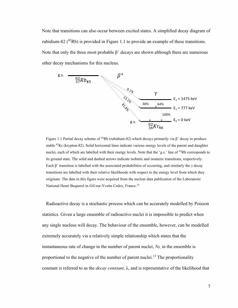
7

Note that transitions can also occur between excited states. A simplified decay diagram of

rubidium-82 (82Rb) is provided in Figure 1.1 to provide an example of these transitions.

Note that only the three most probable β+ decays are shown although there are numerous

other decay mechanisms for this nucleus.

Figure 1.1 Partial decay scheme of 82Rb (rubidium-82) which decays primarily via β+ decay to produce

stable 82Kr (krypton-82). Solid horizontal lines indicate various energy levels of the parent and daughter

nuclei, each of which are labelled with their energy levels. Note that the ‘g.s.’ line of 82Rb corresponds to

its ground state. The solid and dashed arrows indicate isobaric and isomeric transitions, respectively.

Each β+ transition is labelled with the associated probabilities of occurring, and similarly the γ decay

transitions are labelled with their relative likelihoods with respect to the energy level from which they

originate. The data in this figure were acquired from the nuclear data publication of the Laboratoire

National Henri Bequerel in Gif-sur-Yvette Cedex, France.14

Radioactive decay is a stochastic process which can be accurately modelled by Poisson

statistics. Given a large ensemble of radioactive nuclei it is impossible to predict when

any single nucleus will decay. The behaviour of the ensemble, however, can be modelled

extremely accurately via a relatively simple relationship which states that the

instantaneous rate of change in the number of parent nuclei, NP, in the ensemble is

proportional to the negative of the number of parent nuclei.15 The proportionality

constant is referred to as the decay constant, λ, and is representative of the likelihood that

8

the ensemble of nuclei will decay per unit time. This differential relationship is described

below along in with its solution (Eq. 0.1 and Eq. 0.2, respectively), where NP,0 represents

the number of parent nuclei at some reference time t = 0. This differential equation and

its solution represent a specific case of the more general family of equations known as the

Bateman equations which describe decay chains of arbitrary size.16

𝑑𝑁𝑃

𝑑𝑡= −𝜆𝑁𝑝

Eq. 0.1

𝑁𝑃(𝑡) = 𝑁𝑃,0𝑒−𝜆𝑡 Eq. 0.2

The activity of the ensemble is defined as the rate of disintegrations per unit time and is

calculated as the product of NP(t) with the decay constant. A corollary of the relation

described above is that the number of parent nuclei never reaches zero, but rather

approaches this limit asymptotically. It is difficult then to know exactly when the

radioactive sample has completely decayed. A convenient measure of the longevity of a

radioactive sample is its half-life, t1/2, which is defined as the time required for the

activity (and number of parent atoms) of a radioactive sample to decrease by half with

respect to its initial value at t = 0. It can be expressed in terms of the decay constant as

per the following relationship.

𝑡1/2 =

ln (2)

𝜆

Eq. 0.3

1.1.2 Interactions of Radiation with Matter

Within the context of this thesis we are only concerned about the interactions of β-

particles and γ-rays as they pass through a medium and so a review of the interaction

mechanisms of heavier ions or neutrons is not included in this discussion.

9

Since β-decays have multiple reaction products the energies of the emitted β-particles

are polyenergetic and can be characterized by an energy spectrum which ranges from 0

keV to Q. The value of Q is fixed by the difference in mass energies of the parent nucleus

and all the daughter nuclei combined.11 β-particles interact readily with the medium

through which they are travelling due to their mass and charge. Upon each interaction

they transfer some of their kinetic energy to the medium, slowing them down. β-particles

are stopped in a medium once their kinetic energy has been depleted. There are two

principal mechanisms for β-particle interactions: collisional or radiative. Collisional

interactions occur between β-particles and the atomic electrons of the medium and are

described as a Coulomb (electrostatic) scattering process.11 The energy imparted on the

medium through collisional interactions leads either to transferring sufficient kinetic

energy to orbital electrons to liberate them from the atoms to which they’re bound

(ionization) or promoting the orbital electrons to a higher energy orbital of the atomic

structure (excitation).13 Radiative interactions are characterized by the emission of

electromagnetic radiation following the rapid change in velocity of the β-particles due to

Coulomb interactions with atomic nuclei.17 These emissions are commonly referred to as

bremsstrahlung radiation and are the principal mechanism underlying x ray emitting

devices. The stopping power, or rate of energy loss per unit distance, of these collisional

and radiative interactions was first described by Hans Bethe in 1930 and was shown to

depend on the kinetic energy of the β-particle as well as the atomic number of the

absorbing material.18 The collisional interactions typically dominate the energy loss of β-

particles except for those with very high kinetic energy and absorbing media with high

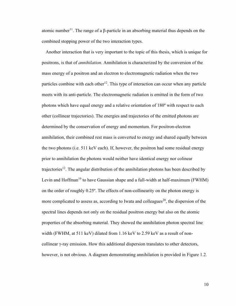
10

atomic number11. The range of a β-particle in an absorbing material thus depends on the

combined stopping power of the two interaction types.

Another interaction that is very important to the topic of this thesis, which is unique for

positrons, is that of annihilation. Annihilation is characterized by the conversion of the

mass energy of a positron and an electron to electromagnetic radiation when the two

particles combine with each other12. This type of interaction can occur when any particle

meets with its anti-particle. The electromagnetic radiation is emitted in the form of two

photons which have equal energy and a relative orientation of 180º with respect to each

other (collinear trajectories). The energies and trajectories of the emitted photons are

determined by the conservation of energy and momentum. For positron-electron

annihilation, their combined rest mass is converted to energy and shared equally between

the two photons (i.e. 511 keV each). If, however, the positron had some residual energy

prior to annihilation the photons would neither have identical energy nor colinear

trajectories12. The angular distribution of the annihilation photons has been described by

Levin and Hoffman19 to have Gaussian shape and a full-width at half-maximum (FWHM)

on the order of roughly 0.25º. The effects of non-collinearity on the photon energy is

more complicated to assess as, according to Iwata and colleagues20, the dispersion of the

spectral lines depends not only on the residual positron energy but also on the atomic

properties of the absorbing material. They showed the annihilation photon spectral line

width (FWHM, at 511 keV) dilated from 1.16 keV to 2.59 keV as a result of non-

collinear γ-ray emission. How this additional dispersion translates to other detectors,

however, is not obvious. A diagram demonstrating annihilation is provided in Figure 1.2.

11

Figure 1.2 Schematic representation of a colinear and non-colinear annihilation of an electron-positron

pair. The energy and momentum of the positron, β+ are indicated as E+ and p+, respectively in the upper

row of the image (“Interaction”). The annihilation photons and their energies are denoted at γ1, γ2, Eγ1,

and Eγ2, respectively in the lower row of the image (“Annihilation”). It is assumed that the electron has

zero kinetic energy and momentum.

Electron interactions occur at a distance due to the fact that both collisional and

radiative interactions are governed by the Coulomb force that exists between charged

objects. The effect is a continual series of interactions as the electron traverses an

absorbing medium. In contrast, photons carry no mass and no electric charge and interact

due to discrete interactions. The most relevant photon interactions for the work described

in this thesis are incoherent (Compton) scatter, and photoelectric absorption. Both of

these interaction pathways result in the conversion of the photon energy to kinetic energy

of an electron. Photoelectric absorption comes about through interactions of photons with

an atom in an absorbing material and results in the complete transfer of the photon energy

to an orbital electron. If the photon energy is greater than the binding energy of the

electron it will be ejected from the atom with kinetic energy equal to the difference of the

photon energy and electron binding energy (ionization). If the photon energy is not

12

greater than the binding energy, the electron can be excited to a higher valence shell of

the atom (excitation). In either event, the incident photon is completely absorbed in the

process.

Incoherent, or Compton, scatter corresponds to an inelastic collision between an

incident photon and an orbital electron wherein the incident photon energy is partially

transferred to the electron. The scattered photon thus has reduced energy compared to the

incident photon and usually undergoes a change in direction. The atom can either be

excited or ionized depending on the amount of energy transferred to the electron in the

process.

The likelihood of either photon interaction depends on the energy of the photon, and

the density and atomic number (Z) of the absorbing material. For photoelectric absorption

the probability of interaction per atom of absorbing material is proportional to the atomic

number raised to the power of ~4 – 5; the exponent varies with photon energy and atomic

number13. The probability of Compton scatter per atom varies (approximately) linearly

with the atomic number17. Photoelectric absorption probabilities per atom are inversely

proportional to the incident photon energy raised to the power of ~3.5. The probability of

Compton scatter, however, has a more complex and much weaker energy dependence.

The Compton scatter likelihood and angular distribution is described by the Klein-

Nishina formula which models the relativistic and quantum mechanical behaviour of this

interaction.17 For an absorber made of water (or soft tissues), the Compton scatter

mechanism dominates over photoelectric absorption for photon energies greater than 30

keV.17

13

1.2 Positron Emission Tomography

Positron emission tomography, or PET, is a molecular imaging modality wherein a

patient is administered a small amount of a chemical agent of biological interest that has

been labeled with an isotope that decays via positron emission which permits the non-

invasive assessment of physiologic processes that are occurring within the body. Such an

agent is referred to as radiotracer. The biochemical nature of the tracer is chosen to target

specific processes and/or organs and to it is attached a radioactive atom that gives rise to

photons that penetrate through the body such that they can be detected externally. PET is

based upon the coincident detection of annihilation photons that are produced following

the β+ decay of a positron-emitting radionuclide of the tracer. Nuclear medicine imaging

procedures, like PET, rely on the so-called tracer principle which assumes that the tracer

is administered in sufficiently small amounts such that is emulates and does not perturb

the natural physiologic processes that are being assessed.21 The term tomography

indicates that the resulting images are arranged as a set of contiguous 2D cross-sectional

slices of the object being imaged. PET images represent an estimate of the spatial

distribution of the positron-emitting radionuclide. The concatenation of the 2D images

thus provides a volumetric representation of this distribution. Within this section the key

aspects of a PET imaging system are described, which include details of the photon

detection systems, the development of PET imaging devices, tomographic image

reconstruction, and data correction techniques that are needed to make PET images

quantitatively accurate.

14

1.2.1 Photon Detection with Scintillators

PET imaging systems detect annihilation photons using an indirect approach based on

scintillating materials. Scintillation materials are those than fluoresce, or emit visible

light, following an interaction with a gamma ray, like an annihilation photon. To allow

for an electronic readout of such a detection, the visible light emitted by the scintillation

crystal must be converted to an electrical signal. The conversion has historically been

achieved in PET detection systems using a device known as a photomultiplier tube

(PMT) but photodiode devices are being increasingly used. A brief description of these

devices will be provided shortly but presently we will return to scintillation materials.

The scintillating materials that have been used in PET systems have largely been

inorganic materials22 and so the description here will be limited to this type. Inorganic

scintillation materials have crystal lattice configurations. An inorganic scintillator’s

properties are largely determined by its structure and the excited states that are accessible

to its valence electrons.13 When excited, however, a valence electron may be elevated to

the conduction band of the crystal at which point it can migrate about the crystal

structure.13 A hole remains within the valence shell that will be filled by the de-excitation

of an electron in the conduction band. The de-excitation process corresponds to the

emission of electromagnetic energy as the electron descends from a higher energy band

to a lower. The energy band in between is the forbidden band and is not accessible to

electrons of pure crystal materials. The energy gap of the forbidden band corresponds to

an electromagnetic emission in the ultra-violet range.22 The crystal material can be

intentionally doped with small amounts of impurities, or activators, which leads to the

establishment of accessible energy levels within the forbidden band.13 The effect of these

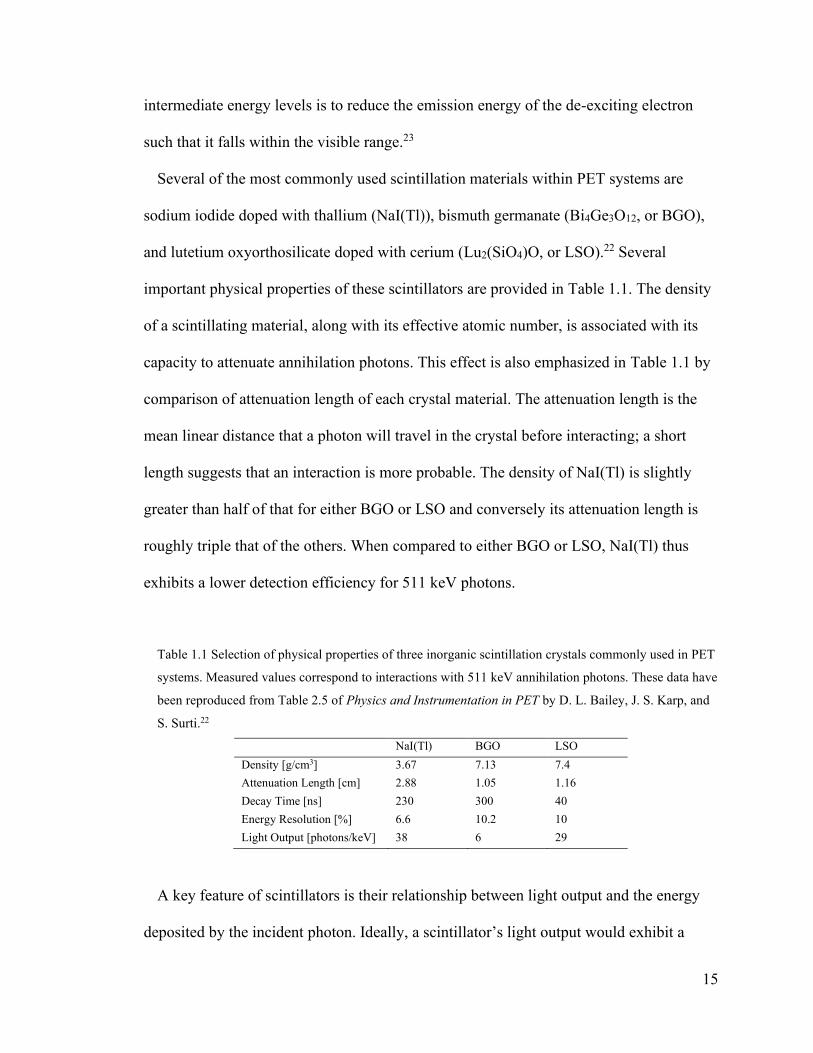
15

intermediate energy levels is to reduce the emission energy of the de-exciting electron

such that it falls within the visible range.23

Several of the most commonly used scintillation materials within PET systems are

sodium iodide doped with thallium (NaI(Tl)), bismuth germanate (Bi4Ge3O12, or BGO),

and lutetium oxyorthosilicate doped with cerium (Lu2(SiO4)O, or LSO).22 Several

important physical properties of these scintillators are provided in Table 1.1. The density

of a scintillating material, along with its effective atomic number, is associated with its

capacity to attenuate annihilation photons. This effect is also emphasized in Table 1.1 by

comparison of attenuation length of each crystal material. The attenuation length is the

mean linear distance that a photon will travel in the crystal before interacting; a short

length suggests that an interaction is more probable. The density of NaI(Tl) is slightly

greater than half of that for either BGO or LSO and conversely its attenuation length is

roughly triple that of the others. When compared to either BGO or LSO, NaI(Tl) thus

exhibits a lower detection efficiency for 511 keV photons.

Table 1.1 Selection of physical properties of three inorganic scintillation crystals commonly used in PET

systems. Measured values correspond to interactions with 511 keV annihilation photons. These data have

been reproduced from Table 2.5 of Physics and Instrumentation in PET by D. L. Bailey, J. S. Karp, and

S. Surti.22

NaI(Tl) BGO LSO

Density [g/cm3] 3.67 7.13 7.4

Attenuation Length [cm] 2.88 1.05 1.16

Decay Time [ns] 230 300 40

Energy Resolution [%] 6.6 10.2 10

Light Output [photons/keV] 38 6 29

A key feature of scintillators is their relationship between light output and the energy

deposited by the incident photon. Ideally, a scintillator’s light output would exhibit a

16

linear relationship with deposited energy over a wide range of energies.13 The energy

resolution of a scintillator is a measure of the precision with which a scintillator (and its

accompanied photodetection system) can identify a discrete photon energy. It is often

calculated as the full width at half-maximum of the energy response divided by the

photon energy being detected and then represented as a percentage. The energy resolution

of NaI(Tl) is better than that of BGO and LSO which has implications for a PET system’s

ability to discriminate between signal and background events. The light output of a

scintillator is also associated with enhanced spatial and coincident timing resolution for

PET systems when multiple scintillation crystals are coupled to a single photodetector.22

The rise and decay times of the scintillator determine the duration over which the

fluorescence occurs. Short rise and decay times are ideal as they result in quick signal

pulses13 which enhances the detector’s capacity to distinguish events that take place in

rapid succession.23 In general, inorganic scintillators exhibit long decay times but LSO

demonstrates a remarkable improvement in decay time over others like NaI(Tl) and

BGO.

An auxiliary device is needed to convert the visible light emitted by scintillators into an

electrical pulse that indicates the detection of a photon; these are generally referred to as

photodetectors. Several important properties of these devices are a high efficiency for

conversion of visible photons to electrons, rapid charge collection and signal readout, and

high amplitude resolution, i.e. high signal gain and low electronic noise.24

Photomultiplier tubes (PMTs) have been widely used for this purpose both in medical

imaging applications as well as in basic nuclear physics.13 PMTs are composed of three

key components: a photocathode, an evacuated electron multiplication chamber, and a

17

pulse-shaping pre-amplifier.24 The photocathode serves as a window between the

scintillator and the PMT and it is triggered by photoelectric interactions of the

scintillation photons to emit electrons.22 If the electrons are energetic enough to escape

the photocathode, they cascade through the evacuated region of the PMT where a high

electric field within the vacuum tube causes the photoelectrons to accelerate. The

electrical signal is insufficient to produce a detectable electrical signal, however, without

an electron multiplication system.13 PMTs achieve signal amplification by accelerating

the initial photoelectrons to collide with a series of targets known as dynodes. A single

electron will stimulate the emission of approximately 6 secondary electrons after a

collision with the dynode.24 It follows that a signal gain on the order of 107 is achievable

with ~10 dynodes.13 The total charge that reaches the anode leads to an electronic pulse

which is shaped by the pre-amplifier prior to further processing of the event. Two

remarkable features of PMTs are their ability to achieve such high signal gain without

introducing significant electronic noise other than the inherent quantum fluctuations of

generating secondary electrons, and they do not dilate the initial pulse width of the

scintillator.13

PMTs have some limiting features which affect the PET system design. Their physical

size imposes restrictions on how densely they can be positioned, which means that

multiple scintillation crystals must be coupled to a single PMT.22 Additionally, PMTs are

highly sensitive to magnetic fields24 which make them incompatible with hybrid PET

scanners integrated with magnetic resonance imaging (MRI) scanners. An alternative

family of photodetectors based on semiconductor diode technology is well suited to

compensate for these disadvantages of PMTs.

18

Diode-type photodetectors, or photodiodes, consist of lamellar combinations of p-type

and n-type semiconductor materials. The type of the semiconductor material is an

indication of its doping and the forms of its charge carriers. P-type semiconductors are

those that are doped with impurities that have one fewer valence electron than the atoms

of the semiconductor material, and as a result these impurities introduce positive charge

carriers in the form of electron holes into the crystal structure.13 Conversely, n-type

materials are doped with impurities that carry an additional valence electron compared to

the atoms of the semiconductor and thus supply negatively charge carriers in the form of

electrons into the material.13 P- and n-type layers are coupled to a pure semiconductor

layer to produce PIN photodiodes, where I in the acronym refers to intrinsic and

corresponds to the pure, undoped, junction region wherein there are no excess charge

carriers. In silicon photodiodes the deposition of roughly 3.6 eV is sufficient to excite

valence electrons and produce electron-hole pairs. The presence of positive and negative

charges at the p- and n-type layers, respectively, causes the electron and hole to drift

away from each other and produce a potential difference within the junction.24 In this

manner visible photons may be detected. Without the application of an external electric

field, PIN photodiodes have no gain and their signals are very sensitive to electronic

noise. Additionally, their pulse width depends on the drift time of the charge carriers

within the intrinsic layer.13 This photodiode design has been modified in a manner to

establish a signal amplification (avalanche) following the production of the initial

electron-hole pair. These avalanche photodiodes (APDs) come in various configurations

but a common one is the reach-through design which consists of a highly doped p-type

entrance layer, a lightly doped p-type drift region, and p-n+ multiplication region.13 The

19

combination of this layered arrangement along with a high external electric field provides

a significant amount of kinetic energy to the electron-hole pairs that are produced from

photon interaction within the drift region which stimulates a run-away cascade of

electron-hole pair production. The typical signal gain achieved with this design is on the

order of hundreds.24 The gain of APDs generally exhibit a linear relationship with the

applied voltage.25

The gain of an APD, however, has higher variability than that on the PMT which can

reduce its energy resolution, but the increased quantum efficiency over PMTs partially

compensates for this effect.13 The gain of photodiodes is also highly sensitive to the

operating temperature and the stability of the high voltage supply and so any system

making use of these photodetectors must be able to control both very precisely.22 Lastly,

the rise-time of the APD pulse can be twice that of common PMTs and can thus improve

the overall timing resolution.24 The APD design has been improved upon by the

development of multi-pixel photon counting (MPPC) photodiodes, a common example of

which is the silicon photomultiplier (SiPM). MPPCs are a structured array of individual

APDs operating at high voltages, typically above 100 V. Under such an external field the

gain takes on steeper, i.e. more sensitive, relationship with the applied voltage but

maintains reasonable linearity.25 The gain associated with SiPM photodetectors is similar

to that of PMTs25 and are typically on the order of 106. In modern PET systems, the

energy resolution of the SiPM photodetectors are comparable to that of PMTs; typically

around 10%.26 The timing resolution of PET systems using SiPMs, however, have

improved over those using PMTs. As an example, the timing resolution of the Philips

Vereos PET/CT (uses SiPMs) and GE Discovery 690 PET/CT (uses PMTs) system have

20

been reported as 332 ps26 and 544 ps27, respectively, and both make use of LYSO

scintillators.

While the photon detection system of the PET scanner is an essential component of is

performance, the PET system itself is much more complex and represents the

combinations of many systems to actually image a patient. In the following section some

of the essential components of a PET system are described.

1.2.2 PET System Design and Performance

The purpose of a PET acquisition is to produce an image, or spatial description, of the

radiotracer concentration within a patient. Such an image is produced by solving the

following inverse problem: How can we determine the radiotracer distribution from the

emission data detected by the PET scanner? It turns out the this problem is not unique to

PET, nor medical imaging, and various analytic and iterative methods exist that can

provide a solution.28 More detail will be provided in the following section on the image

reconstruction problem in PET, but for now it is relevant to mention that solving these

problems requires that the emission data is sufficiently sampled about the object being

imaged.28 In PET sufficient sampling is achieved by arranging a set of detectors along a

circular gantry that encompasses the patient. While some systems employ partial ring or

flat panel detectors that rotate about the patient, most use full ring configurations.29

Regardless of the configuration the detectors must be arranged such that they oppose

each other to permit the detection of collinear annihilation photons. A schematic

representation of full ring, multi-slice configuration is shown in Figure 1.3. In this

illustration, the coordinate system in the full-ring scanner is indicated along with a single

21

line-of-response emanating from the annihilation location within the patient which is

marked by a lightning bolt.

Figure 1.3 Schematic representation of a full-ring multi-slice PET detector configuration. Cross-sectional

views from the front face of the gantry and from the side are shown in sub-figures A, and B,

respectively. Each gray rectangle represents a detector. In sub-figure A, the transverse coordinate

directions, x, and y, are depicted by dashed lines. The transverse origin is shown as a circle at the

intersection of the x and y axes. A line of response (LOR), which originates at the position marked by the

lightning bolt, subtends an azimuthal angle φ with the positive y axis. A model patient is represented by

the blue ellipse. In sub-figure B, the span of axial direction, or z axis, is shown. The same LOR subtends

a polar angle θ with the positive z axis. The vector 𝑠(𝑠, 𝑢) describes the position of the LOR.

The detector elements have also been designed with various configurations. One of the

most successful detector designs is that of the block detector.29 In this design, a

rectangular grid of individual scintillation crystals is optically coupled to a set of photo-

detectors with a relatively high ratio of the number of individual crystals to photo-

detectors; 64:4, for example, as depicted in Figure 1.4.

22

Figure 1.4 Arrangement of 64 scintillation crystal elements and 4 PMTs in detector block design. The

block quadrants A, B, C, and D correspond to unique PMTs.

While it is not shown in Figure 1.4, the divisions between individual elements are often

incomplete and reflective barriers exist in these regions to help guide scintillation light

towards the PMTs and impose limits on the spatial dispersion. By varying the lengths of

the reflective barriers across the block, a different amount of light reaches each of the

attached PMTs which helps to identify the crystal from which the scintillation occurred.29

The x and y coordinates of the scintillation can be estimated using the relative pulse-

heights of the four PMTs (A, B, C, and D) as shown in Eq. 0.4 and Eq. 0.5, commonly

referred to as Anger logic, after its originator Hal Anger.29 In the block detector design,

all four PMTs are occupied over the span of time that is takes to resolve a single event.

This has an impact on the scanner’s sensitivity to detection annihilation photons,

especially when the count rate is high.

𝑥 =

(𝐵 + 𝐷) − (𝐴 + 𝐶)

𝐴 + 𝐵 + 𝐶 + 𝐷

Eq. 0.4

𝑦 =

(𝐴 + 𝐵) − (𝐶 + 𝐷)

𝐴 + 𝐵 + 𝐶 + 𝐷

Eq. 0.5

23

A single coincident event is described by the crystal indices of each photon detection as

well as the time at which the event occurred. Two photons are considered to be in

coincidence if they are detected within a relatively short period of time, i.e. within the

coincidence window (2τ). The duration of the coincidence window is partially limited by

the timing resolution of the detectors which, as described in the previous section, is

associated with the rise time of the scintillators and the pulse dispersion of the

photodetectors. Additionally, the geometry of the scanner must also be considered when

determining an appropriate timing window as the time it takes each annihilation photon

to reach a detector may differ due to the difference in distances each photon must traverse

(at the speed of light). As an example, while a timing resolution of 0.6 ns has been

reported for a barium fluoride (BaF2) PET system30, a timing difference of up to 3 ns

could be expected for annihilation photons in a very large patient, and so setting a

coincidence window based on the timing resolution alone would limit the overall

sensitivity of the scanner.22 For PET systems that make use of fast scintillators and

electronics which have timing resolution < 0.6 ns, the timing delays of the coincidence

photons can be resolved sufficiently well to infer where along the LOR the annihilation

occurred31. Recording the time difference between detection of coincident photons is

referred to as the time-of-flight (TOF) of the coincidence event. The position of an

annihilation event, with respect to the middle point of the LOR, can be calculated as

𝑐∆𝑡 2⁄ , where ∆𝑡 is the time delay between the arrival times of the two annihilation

photons and c is the speed of light in air. A timing resolution of 500 ps thus corresponds

to a spatial resolution of 7.5 cm of the annihilation event along the LOR. The benefit of

24

the use of TOF data lies in improved noise characteristics in the reconstructed image.22

Interestingly, if the timing resolution was sufficiently small such that the spatial

uncertainty of the annihilation event along the LOR was smaller than the spatial

resolution of the system, no image reconstruction would be required.32

In the following sections spatial resolution, energy resolution, timing resolution, count

rate performance, and sensitivity are described.

1.2.2.1 Spatial Resolution

The spatial resolution of an imaging system is a measure of the smallest separation

between objects that can be discerned in an image and is often measured as the FWHM of

a small object representation in an image.29 Note that for an object to be considered

small, it should be no larger than half the size of the spatial resolution of the system.29

There are various factors which affect the spatial resolution of the system: positron range,

non-collinearity of the annihilation photons, sizes and separation of detectors, variance in

the depth into a crystal (depth-of-interaction) where the ionization occurs31, and block-

detector decoding in the case of the multi-crystal block configuration. In most full-ring

systems the spatial resolution in the transverse plane (x-y) is smaller than that in the axial

direction (z) as the transverse field of view is oversampled compared to along the axial

direction.29 See Table 1.2 for example measurements; the “Radial” and “Tangential”

measurements are made in-plane while the “Axial” measurements are along z. The

spatial resolution of a PET system fundamentally limits its ability to determine the spatial

distribution of a radiotracer within a patient.

25

1.2.2.2 Energy Resolution

The energy resolution of the system is associated with the precision with which a

detector can determine the energy of detected photons.29 In addition to the emission of a

positron during the decay of the radiotracer, other prompt gamma ray emission or

scattered annihilation photons may be detected that lead to increased noise and/or

artifacts in the reconstructed images. Some of these types of photons are excluded from

the emission data through energy discrimination.

1.2.2.3 Timing Resolution

Good timing resolution, as was mentioned, is important for identifying coincidence

events and, with sufficiently fast crystals and electronics, for TOF measurement as well.

In terms of system performance, a narrower coincidence window helps to exclude

random coincidence events that arise from simultaneous detection of two independent

annihilation photons. Random coincidences lead to a uniform increase in the background

which can reduce the contrast in the resulting image as they carry no useful spatial

information and occur stochastically within the field of view.22 The rate of detecting

random coincidences is proportional to the width of the coincident window and the

square of the activity in the field-of-view of the scanner.29

1.2.2.4 Dead Time and Count Rate Performance

Once a detector is triggered by the detection of a photon, there is a period wherein no

additional events can be registered. This time is referred to as dead time and is associated

with the time needed for the scintillator’s response, the electronic response of the

photodetector, the integration time of the electronics, and time associated with processing

26

coincidence events. The count rate performance of a PET system is an indicator of its

ability to process detection events over a broad range of system count rates, or activity in

the field-of-view. The dead time is a non-linear function of the count rate of the system

and is composed of two contributions: paralyzable and non-paralyzable dead times.33 In

the non-paralyzable case, the detector is unresponsive to events that occur within a fixed

time τ following a detection; subsequent events are ignored and have no further effect on

the detector.13 Paralyzable dead time, however, implies that all events lead to a dead time

τ, even if they occur while the detector is ‘dead’ from an initial event.13 Paralyzable dead

time can lead to saturation of the detector wherein the system count rate can decrease in

the presence of an increasing event rate.33 Dead-time corrections must be applied in PET

to achieve linear response over the broad range of count-rates so that resulting images can

accurately quantify activity concentrations in the subject.

There are three types of coincidence events PET systems detect: true coincidences of

annihilation photon pairs, coincidence of photons that have scattered and random

coincidences of two photons from two separate decay events. While true coincidence

events are the desired signal in PET, the scatter and random events are unavoidable and

degrade image quality. A common measure of the count rate performance of a PET

system is the noise equivalent count rate (NECR). This metric is defined as the count rate

of true coincidence events that would give the same signal-to-noise ratio as the real count

rate of the system in the absence of random and scattered coincidence events.29

Mathematically it is calculated as shown below (Eq. 0.6), where T, S, and R represent the

count rates of the true, scattered, and random coincidence events, respectively.34 The

factor K is used to accommodate different methods of correction for random coincidence

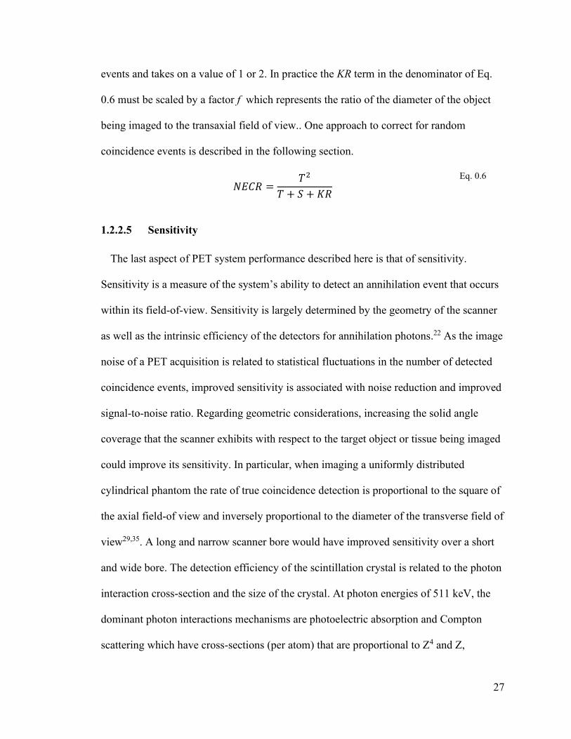
27

events and takes on a value of 1 or 2. In practice the KR term in the denominator of Eq.

0.6 must be scaled by a factor f which represents the ratio of the diameter of the object

being imaged to the transaxial field of view.. One approach to correct for random

coincidence events is described in the following section.

𝑁𝐸𝐶𝑅 =

𝑇2

𝑇 + 𝑆 + 𝐾𝑅

Eq. 0.6

1.2.2.5 Sensitivity

The last aspect of PET system performance described here is that of sensitivity.

Sensitivity is a measure of the system’s ability to detect an annihilation event that occurs

within its field-of-view. Sensitivity is largely determined by the geometry of the scanner

as well as the intrinsic efficiency of the detectors for annihilation photons.22 As the image

noise of a PET acquisition is related to statistical fluctuations in the number of detected

coincidence events, improved sensitivity is associated with noise reduction and improved

signal-to-noise ratio. Regarding geometric considerations, increasing the solid angle

coverage that the scanner exhibits with respect to the target object or tissue being imaged

could improve its sensitivity. In particular, when imaging a uniformly distributed

cylindrical phantom the rate of true coincidence detection is proportional to the square of

the axial field-of view and inversely proportional to the diameter of the transverse field of

view29,35. A long and narrow scanner bore would have improved sensitivity over a short

and wide bore. The detection efficiency of the scintillation crystal is related to the photon

interaction cross-section and the size of the crystal. At photon energies of 511 keV, the

dominant photon interactions mechanisms are photoelectric absorption and Compton

scattering which have cross-sections (per atom) that are proportional to Z4 and Z,

28

respectively, where Z is the atomic number of an atom in the scintillator.23 More

generally, increased effective atomic number and density within a polyatomic scintillator

leads to increased intrinsic detection efficiency and thus scanner sensitivity.

1.2.2.6 Performance Characteristics of GE Discovery 690 PET/CT System

The work described in this thesis largely made use of the Discovery 690 (D690) PET

system developed by General Electric (GE) Healthcare (Waukesha, WI), which is a PET

system with first generation time-of-flight capability. Performance characteristics of this

system were reported by Bettinardi and colleagues27 following the 2007 National

Electrical Manufacturers Association (NEMA) standards for positron emission

tomographs. The D690 is a hybrid PET system that includes a 64-slice CT scanner

mounted at the front of the PET scanner gantry. This PET scanner contains 13,824

lutetium yttrium orthosilicate (LYSO) crystals as scintillators. The crystal dimensions are

4.2 × 6.3 × 25 mm3. The detector units are of the block design style and each contains 54

(9 × 6) individual crystals. Each block uses only a single position-sensitive

photomultiplier tube with four anodes. The blocks are positioned within rectangular

module units that hold 8 blocks, two transverse by four axial blocks. In total 32 blocks

complete the full ring of the detection system. The axial and transverse field-of-view are

157 mm and 700 mm, respectively. The performance measurements data are provided in

Table 1.2.

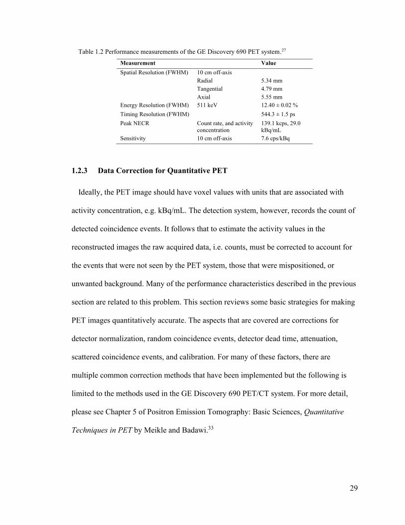
29

Table 1.2 Performance measurements of the GE Discovery 690 PET system.27

Measurement Value

Spatial Resolution (FWHM)

10 cm off-axis

Radial

Tangential

Axial

5.34 mm

4.79 mm

5.55 mm

Energy Resolution (FWHM) 511 keV 12.40 ± 0.02 %

Timing Resolution (FWHM) 544.3 ± 1.5 ps

Peak NECR Count rate, and activity

concentration

139.1 kcps, 29.0

kBq/mL

Sensitivity 10 cm off-axis 7.6 cps/kBq

1.2.3 Data Correction for Quantitative PET

Ideally, the PET image should have voxel values with units that are associated with

activity concentration, e.g. kBq/mL. The detection system, however, records the count of

detected coincidence events. It follows that to estimate the activity values in the

reconstructed images the raw acquired data, i.e. counts, must be corrected to account for

the events that were not seen by the PET system, those that were mispositioned, or

unwanted background. Many of the performance characteristics described in the previous

section are related to this problem. This section reviews some basic strategies for making

PET images quantitatively accurate. The aspects that are covered are corrections for

detector normalization, random coincidence events, detector dead time, attenuation,

scattered coincidence events, and calibration. For many of these factors, there are

multiple common correction methods that have been implemented but the following is

limited to the methods used in the GE Discovery 690 PET/CT system. For more detail,

please see Chapter 5 of Positron Emission Tomography: Basic Sciences, Quantitative

Techniques in PET by Meikle and Badawi.33

30

1.2.3.1 Normalization correction

Normalization correction corresponds to correcting for non-uniformities in the intrinsic

detection efficiencies of individual crystals, geometric effects, structural misalignment of

the detectors, and asynchronous timing between detector pairs.33 Intrinsic detection

efficiencies may vary due to crystal non-uniformity or variations in photodetector gain.

Additionally, the transverse and axial positions of a crystal within a block may also affect

its sensitivity (transverse and axial block profile corrections). Geometric factors consider

solid angle coverage and incident angles of detected photons for individual crystal, which

vary depending on the acceptance angle of the coincidence system as well as the location

of the emission within the FOV. These efficiency components are typically determined

using measurements of rod and cylinder sources with uniform activity concentration.33

Moreover, the acquisitions use low amounts of activity and are long in duration to make

measurements that have low noise and to mitigate dead time effects.33

1.2.3.2 Random Coincidence Correction

For a given detector pair, the rate of random coincidence events can be calculated as

the product of the coincidence window, 2τ, with the non-coincident, or singles, detection

rates of the two detectors.31 The total number of random coincidence events in an

acquisitions can be estimated by the integral of the random coincidence detection rate

over the duration of the acquisition. Prior to reconstruction the total number of random

coincidence events, once corrected for radioactive decay, can be subtracted, for each

detector pair, to compensate for their effect on the image. This estimation method

assumes that the response of every detector pair is uncorrelated and that the spatial

distribution of the activity is effectively fixed over time.33 Generally, the singles rates

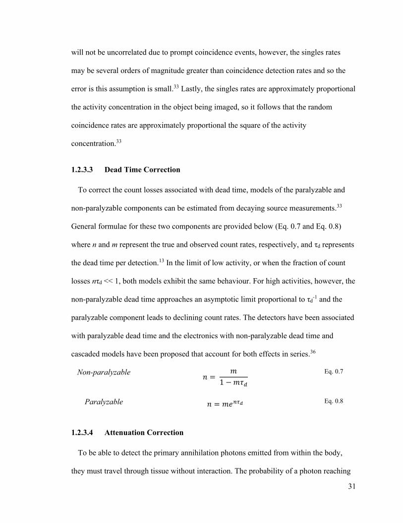
31

will not be uncorrelated due to prompt coincidence events, however, the singles rates

may be several orders of magnitude greater than coincidence detection rates and so the

error is this assumption is small.33 Lastly, the singles rates are approximately proportional

the activity concentration in the object being imaged, so it follows that the random

coincidence rates are approximately proportional the square of the activity

concentration.33

1.2.3.3 Dead Time Correction

To correct the count losses associated with dead time, models of the paralyzable and

non-paralyzable components can be estimated from decaying source measurements.33

General formulae for these two components are provided below (Eq. 0.7 and Eq. 0.8)

where n and m represent the true and observed count rates, respectively, and τd represents

the dead time per detection.13 In the limit of low activity, or when the fraction of count

losses nτd << 1, both models exhibit the same behaviour. For high activities, however, the

non-paralyzable dead time approaches an asymptotic limit proportional to τd-1 and the

paralyzable component leads to declining count rates. The detectors have been associated

with paralyzable dead time and the electronics with non-paralyzable dead time and

cascaded models have been proposed that account for both effects in series.36

Non-paralyzable 𝑛 =

𝑚

1 − 𝑚𝜏𝑑

Eq. 0.7

Paralyzable 𝑛 = 𝑚𝑒𝑛𝜏𝑑 Eq. 0.8

1.2.3.4 Attenuation Correction

To be able to detect the primary annihilation photons emitted from within the body,

they must travel through tissue without interaction. The probability of a photon reaching

32

the detector without being absorbed or scattered depends on the attenuating effect of all

the materials that exist along a linear trajectory toward the detector. The attenuating

effect of a given material or tissue type can be described by its linear attenuation

coefficient μ. This value represents the combined likelihoods of the photon interacting

through all of the mechanisms described in Section 1.1.2 and is interpreted as the

probability per unit length of an interaction occurring that removes the photon from its

original trajectory. If attenuation is not taken into account PET images will appear to

have reduced intensity in regions of high attenuation or regions which have a longer

pathlength in tissue before the photon emerges from the body (i.e. deep anatomical

regions).

It may be surprising to learn that to correct for this effect in PET acquisitions we do not

require knowledge of the annihilation point along a LOR. This convenient aspect of a

PET acquisition, which simplifies the process of correcting attenuation, falls from the fact

that only coincident photon detections are used as signal. Consider a LOR which spans a

distance L between two detectors and that the annihilation occurred at a distance x from

the first detector. The path lengths of the two photons are thus x and L – x and the

probabilities of each photon reaching the corresponding detectors are shown in Eq. 0.9

and Eq. 0.10 below,

𝑝1 = 𝑒− ∫ 𝜇(𝑥′)𝑥

0 𝑑𝑥′

Eq. 0.9

𝑝2 = 𝑒− ∫ 𝜇(𝑥′)𝐿

𝑥𝑑𝑥′

Eq. 0.10

where 𝜇(𝑥′) is the attenuation coefficient at any position 𝑥′. The likelihood (𝑝) of a

coincidence detection of these two independent events is thus given as the product of 𝑝1

and 𝑝2, shown in Eq. 0.11, which has no dependence on the annihilation position x.

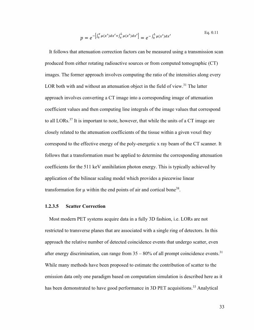
33

𝑝 = 𝑒−[∫ 𝜇(𝑥′)

𝑥0 𝑑𝑥′+∫ 𝜇(𝑥′)

𝐿𝑥 𝑑𝑥′] = 𝑒− ∫ 𝜇(𝑥′)

𝐿0 𝑑𝑥′

Eq. 0.11

It follows that attenuation correction factors can be measured using a transmission scan

produced from either rotating radioactive sources or from computed tomographic (CT)

images. The former approach involves computing the ratio of the intensities along every

LOR both with and without an attenuation object in the field of view.31 The latter

approach involves converting a CT image into a corresponding image of attenuation

coefficient values and then computing line integrals of the image values that correspond

to all LORs.37 It is important to note, however, that while the units of a CT image are

closely related to the attenuation coefficients of the tissue within a given voxel they

correspond to the effective energy of the poly-energetic x ray beam of the CT scanner. It

follows that a transformation must be applied to determine the corresponding attenuation

coefficients for the 511 keV annihilation photon energy. This is typically achieved by

application of the bilinear scaling model which provides a piecewise linear

transformation for μ within the end points of air and cortical bone38.

1.2.3.5 Scatter Correction

Most modern PET systems acquire data in a fully 3D fashion, i.e. LORs are not

restricted to transverse planes that are associated with a single ring of detectors. In this

approach the relative number of detected coincidence events that undergo scatter, even

after energy discrimination, can range from 35 – 80% of all prompt coincidence events.31

While many methods have been proposed to estimate the contribution of scatter to the

emission data only one paradigm based on computation simulation is described here as it

has been demonstrated to have good performance in 3D PET acquisitions.33 Analytical

34

simulation of the scatter process requires knowledge of the attenuation along each LOR,

an estimate of the scatter free activity distribution, detector efficiencies and solid angle

coverage and a model of the differential cross-section of scatter interactions.39 For some

non-linear, iterative, reconstruction algorithms the scatter estimates are produced and

subtracted from the emission data following correction for normalization but prior to

image reconstruction.40 Other algorithms incorporate scatter estimates into the

reconstruction process as a separate contribution to the observed counts. Scatter

correction based on this simulated approach may be implemented in the following steps:

reconstruct an attenuation image, e.g. from a CT image; reconstruct an initial, low

resolution, emission image; perform scatter simulation and estimate the scatter

contribution to the emission data; scale the scatter estimates to match the emission image

outside of the object being imaged, i.e. in the region where only scatter can exist; and

finally, subtract the scatter estimate from the emission data.33 The operation of scaling the

scatter estimates to the emission image in the regions outside of the body has implications

to the methods proposed in this thesis, as is discussed in Chapter 3 and Chapter 6.

Once all of the previously mentioned corrections are applied all that remains is to

verify that activity measured in the PET images is in agreement with the activity

measurements made in a calibrated well counter.33 This procedure could be performed by

imaging a phantom which contains a uniform distribution of activity and measuring the

activity from a sample drawn from the phantom in a well counter.33 If discrepancies exist

between the PET image and well-counter measurements a well-counter correction factor

can be applied to scale the PET images to report quantitatively accurate values, typically

in units of Bq/cc.

35

1.2.4 Tomographic Image Reconstruction

As was mentioned at the beginning of the last section, image tomographic image

reconstruction is an inverse problem for which there are various available solutions. In

modern PET systems the most employed solutions are iterative processes wherein the

solution, i.e. the image, is updated and refined repeatedly until a satisfactory result is

reached. While analytical solutions, namely filtered back-projection, may still be used,

and indeed can provide valuable insight into image reconstruction processes, they are not

described here. This description will be limited to that of the maximum likelihood

expectation maximation (MLEM)41 method as applied to PET.42

Before describing the reconstruction method, it is useful to consider the format of the

PET emission data. In its most basic form, the PET data are stored in a format where each

coincident detection is simply written to file. In this so-called list-mode data, each event

is described (at least) in terms of indicators of the two detectors that observed the event as

well as the time at which the event occurred. Additional events may be written to the list-

mode data like scheduled time stamp events or trigger events. Triggers are indicators of

the state of the patient being imaged and could, for example, mark the beginning of each

cardiac cycle that the patient experiences during the acquisition. Triggers are produced by

some sort of system which monitors the physiological process of the patient, e.g. an

electro-cardiogram (ECG) is used to monitor cardiac contraction. Triggers are described

in detail in Section 2.3.2. The list-mode format is often inconvenient for the purposes of

image reconstruction as it is not easily adapted for traditional analytic reconstruction

algorithms and also imposes significant data storage requirements as the number of

detected coincidence events can be on the order of ~108 for a PET acquisition.43

36

More commonly, the individual detected events are combined into a series of

histograms where each corresponds to a parallel set of LORs that form a plane that

intersects the FOV at an orientation �� specified by azimuthal (𝜑) and polar (𝜃) angles

about the geometric center of the scanner. Each histogram is referred to as a projection of

the activities along a parallel set of LORs. The number of counts in each bin corresponds

to the value of the line integral of the tracer distribution along the LOR within the object

being imaged. Each bin center of the histogram is described by a vector 𝑠 = (𝑠, 𝑢) for a

given projection angle. This notation is consistent with that shown earlier in Figure 1.3,

but here a parallel set of LORs in considered instead of just one. The set of all projections

at all angles subtended by the support of the PET detection system is referred to as a

sinogram. A diagram which describes a single sinogram element 𝑝 = (𝑠, 𝜑, 𝑢, 𝜃) of an

eccentric cylinder filled with activity is shown in Figure 1.5. Since the activity

distribution is completely described by only three independent variables, e.g. x, y, and z,

the projections thus contain redundant information which help to improve the overall

sensitivity of the scanner and the signal-to-noise ratio in the reconstructed images.29

The image reconstruction process is effectively a computation of the activity

distribution that gave rise the detected projection data given a (forward) model of the

imaging system which relates these two data sets. This problem is discrete as we cannot

determine continuous distributions of the either the projection data or the image data. It

follows that projection and image data can be organized as 1D vectors �� and 𝑓,

respectively. The imaging system can be represented as a matrix 𝐻 which operates on the

image data 𝑓 to generate the projection data ��. If the image and projection data contain N

and M elements, respectively, then H is given as an M × N matrix and is referred to as the

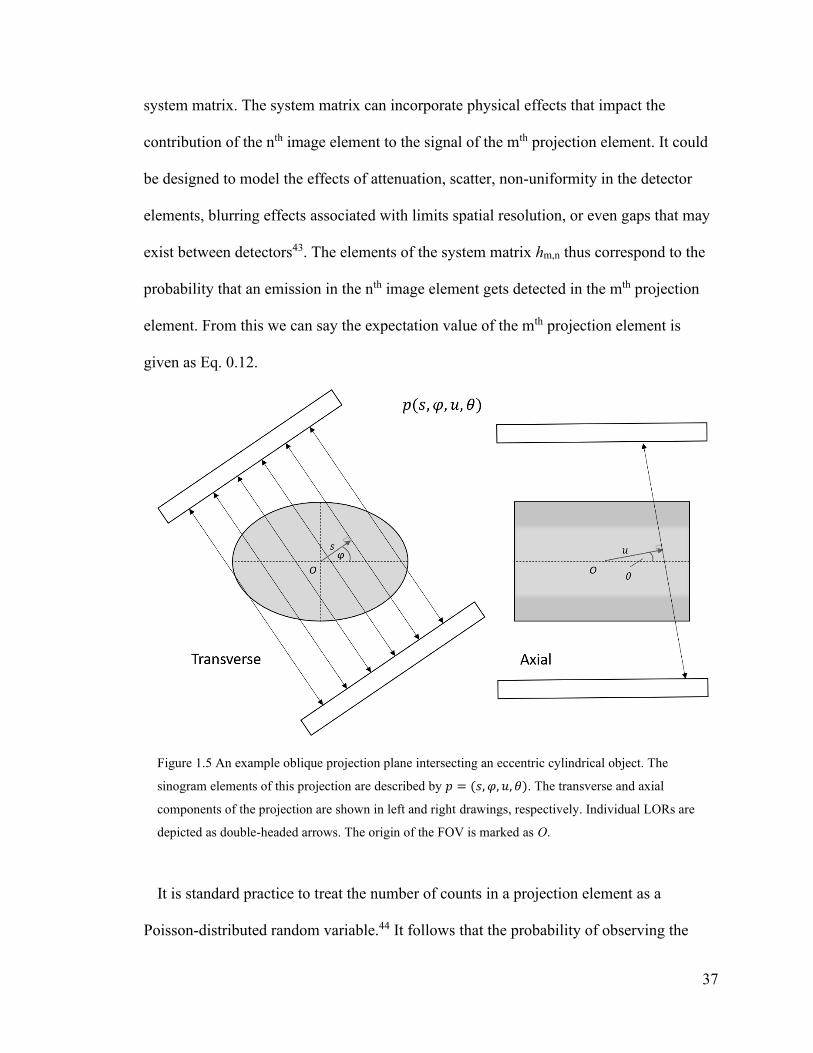
37

system matrix. The system matrix can incorporate physical effects that impact the

contribution of the nth image element to the signal of the mth projection element. It could

be designed to model the effects of attenuation, scatter, non-uniformity in the detector

elements, blurring effects associated with limits spatial resolution, or even gaps that may

exist between detectors43. The elements of the system matrix hm,n thus correspond to the

probability that an emission in the nth image element gets detected in the mth projection

element. From this we can say the expectation value of the mth projection element is

given as Eq. 0.12.

Figure 1.5 An example oblique projection plane intersecting an eccentric cylindrical object. The

sinogram elements of this projection are described by 𝑝 = (𝑠, 𝜑, 𝑢, 𝜃). The transverse and axial

components of the projection are shown in left and right drawings, respectively. Individual LORs are

depicted as double-headed arrows. The origin of the FOV is marked as O.

It is standard practice to treat the number of counts in a projection element as a

Poisson-distributed random variable.44 It follows that the probability of observing the

38

projection data �� given a tracer distribution 𝑓 is the product of the individual

probabilities over all M projection elements, as shown in Eq. 0.13.

⟨𝑔𝑚⟩ = ∑ ℎ𝑚,𝑛

𝑁

𝑛=1

𝑓𝑛

Eq. 0.12

𝑃𝑟(��|𝑓) = ∏𝑒−⟨𝑔𝑚⟩⟨𝑔𝑚⟩𝑔𝑚

𝑔𝑚!

𝑀

𝑚=1

Eq. 0.13

Here the notation ⟨𝑔𝑚⟩ is used to denote the expectation value of the mth projection

element. The MLEM method42 seeks to estimate the image 𝑓 that maximizes the log-

likelihood function ℒ(𝑓), which is given as Eq. 0.14.43 Note that in this expression, terms

that do not depend on the image elements 𝑓𝑛 are discarded as they will not affect the

estimate of 𝑓 as the log-likelihood is maximized through differentiation with respect to

𝑓𝑛.

ℒ(𝑓) = ∑ [− ∑ ℎ𝑚,𝑛𝑓𝑛 + 𝑔𝑚𝑙𝑜𝑔 (∑ ℎ𝑚,𝑛𝑓𝑛

𝑁

𝑛=1)

𝑁

𝑛=1]

𝑀

𝑚=1

Eq. 0.14

The MLEM method is employed for problems which involve incomplete data where a

closed form solution of the standard maximum likelihood calculation does not exist and

thus needs to be estimated iteratively.41 Typically, the first estimate of image elements

𝑓𝑛𝑖=0 = 1 for 𝑛 ∈ [1, 𝑁]. The image updates thereafter are described in Eq. 0.15.43

𝑓𝑛𝑖+1 = 𝑓𝑛

𝑖1

∑ ℎ𝑚′,𝑛𝑀𝑚′=1

∑ ℎ𝑚,𝑛

𝑔𝑚

∑ ℎ𝑚,𝑛′𝑓𝑛′𝑖𝑁

𝑛′=1

𝑀

𝑚=1

Eq. 0.15

This update step determines a ratio of the observed projection data 𝑔𝑚with the projection

data that one would expect from current image estimate, ∑ ℎ𝑚,𝑛′𝑓𝑛′𝑖𝑁

𝑛′=1 and then maps

that ratio to a factor that modifies the nth image element.

39

The MLEM algorithm guarantees convergence as the number of iterations approaches

infinity as the log-likelihood can be shown to be increase monotonically upon each

iteration.43 While a large number of iterations leads to an unbiased image estimate it also

leads to high noise. This is primarily due to the fact the emission data are inherently noisy

and so the image estimate that maximizes the consistency with the projection data are

also noisy.44 In practice this is addressed by applying post-reconstruction smoothing,

reducing the number of iterations, or imposing regularization in the likelihood function

that enforces smoothness.43 As a final comment, the MLEM method requires the use of

the entire projection data set to complete a single iteration which limits its usefulness in a

clinical environment due to the duration of the reconstruction. To remedy this, a

modification of the original method was proposed by Hudson and Larkin45 wherein only

a subset of the projection data are used for each update which leads to an acceleration of

the reconstruction. If, for example, the projection data were partitioned into five subsets,

each of which are assumed to uniformly sample the projection data, then the

reconstruction would be accelerated by a factor of five. This acceleration comes at the

cost of no longer having guaranteed convergence to the ML image estimate and noise

propagates into the image at an accelerated rate compared to MLEM.44 An example

sinogram and reconstructed transverse image are shown in Figure 1.6 where the sinogram

corresponds to a set of projection planes which were perpendicular to the z-axis of the

system, i.e. θ = 0. These data were collected as part of the work described in Chapter 4

and correspond to an acquisition of an anthropomorphic torso phantom with a cardiac

insert. As you regard the sinogram from its base to its top, you will notice that objects

that are not perfectly aligned in the center of rotation exhibit a sinusoidal trajectory, and

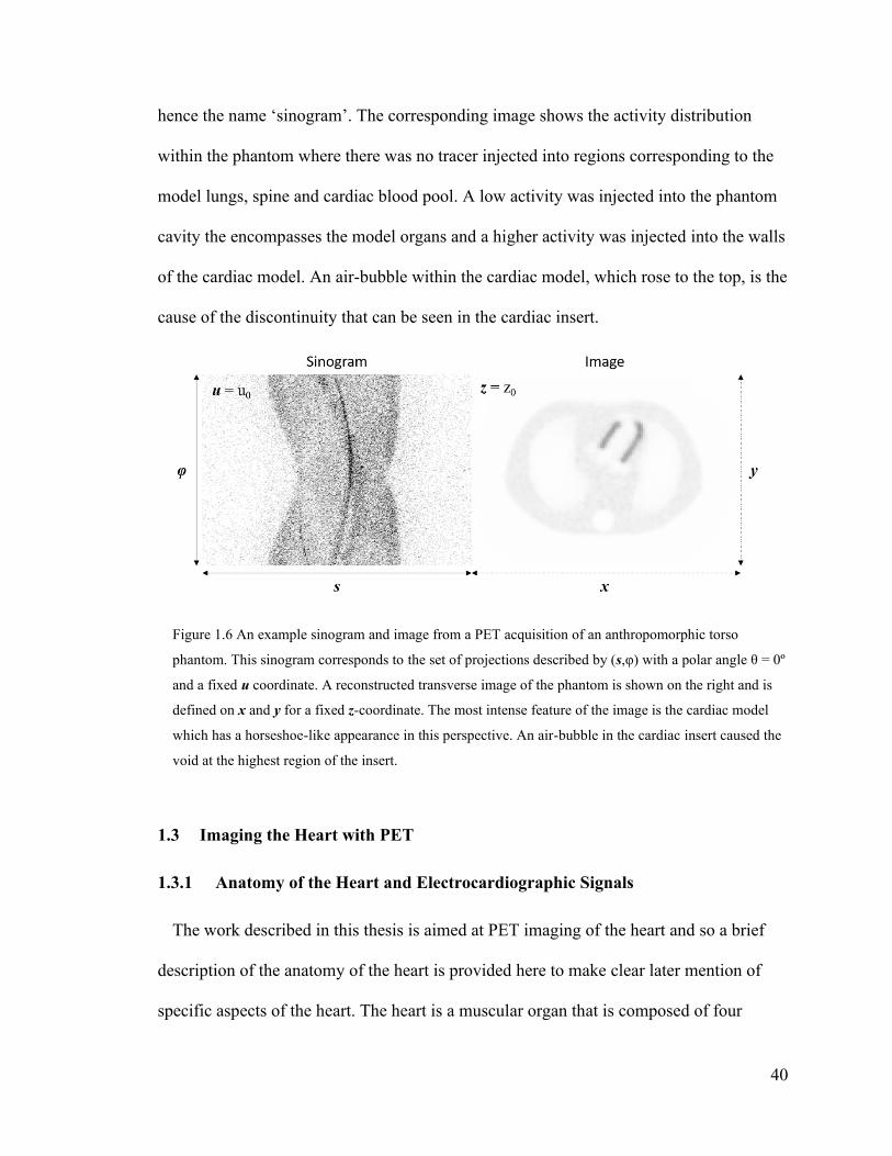
40

hence the name ‘sinogram’. The corresponding image shows the activity distribution

within the phantom where there was no tracer injected into regions corresponding to the

model lungs, spine and cardiac blood pool. A low activity was injected into the phantom

cavity the encompasses the model organs and a higher activity was injected into the walls

of the cardiac model. An air-bubble within the cardiac model, which rose to the top, is the

cause of the discontinuity that can be seen in the cardiac insert.

Figure 1.6 An example sinogram and image from a PET acquisition of an anthropomorphic torso

phantom. This sinogram corresponds to the set of projections described by (s,φ) with a polar angle θ = 0º

and a fixed u coordinate. A reconstructed transverse image of the phantom is shown on the right and is

defined on x and y for a fixed z-coordinate. The most intense feature of the image is the cardiac model

which has a horseshoe-like appearance in this perspective. An air-bubble in the cardiac insert caused the

void at the highest region of the insert.

1.3 Imaging the Heart with PET

1.3.1 Anatomy of the Heart and Electrocardiographic Signals

The work described in this thesis is aimed at PET imaging of the heart and so a brief

description of the anatomy of the heart is provided here to make clear later mention of

specific aspects of the heart. The heart is a muscular organ that is composed of four

41

chambers: the right (RA) and left atria (LA), and the right (RV) and left ventricles (LV).

A cross-sectional diagram of the heart is shown in Figure 1.7 wherein all four chambers

of the heart are depicted. The atria serve as inlet chambers of blood returning to the heart

from elsewhere in the body. In particular, the right atrium is filled by blood from the

superior and inferior vena cava which return de-oxygenated blood from, roughly, above

and below the shoulders, respectively. The left atrium is filled with oxygenated blood

returning the from lungs via the pulmonary veins. Blood passes from each atrium through

a one-way valve into the corresponding ventricle. The right atrium and ventricle are

separated by the tricuspid valve and the left atrium is separated from the left ventricle by

the mitral valve. The right ventricle pushes deoxygenated blood to the lungs via the

pulmonary arteries upon passing through the pulmonary valve. The left ventricle pushes

blood through the aortic valve to the rest of the body via the aorta.

The walls of the heart are a three-layered structure. From the interior to the exterior, the

layers are the endo-, myo-, and pericardium.46 The myocardium contains the muscle cells

that control cardiac contractions. The thickness of the myocardium, which varies

throughout the heart, is associated with the amount of force needed by each chamber to

perform its function.46 The atria are thin structures as they need only push blood into their

adjacent ventricles. The right ventricle (RV) is responsible for driving blood to the lungs,

and back, and it has a thicker myocardium than the atria. The left ventricle has the

thickest myocardium as it must push blood throughout the entire body.

42

Figure 1.7 Basic anatomical diagram of the heart containing the four chambers, valves and major veins

and arteries. This figure has been reproduced from the public domain clipart repository WPClipartiv. The

file was accessed on February 10, 2020.

Blood is supplied to the heart tissue via the right and left coronary arties which

originate at the base of the aorta. Both the right and left coronary arteries sub-divide

fractally to supply blood to all regions of the heart. The major coronary arteries, and

which are relevant to this work, are the left-anterior descending (LAD), left-circumflex

(LCX), and right coronary (RCA) arteries. These three arteries supply blood to the left

ventricle, which, as will be described in the following section, is the primary imaging

iv WPClipart: https://www.wpclipart.com/medical/anatomy/heart/heart_diagram.png.html

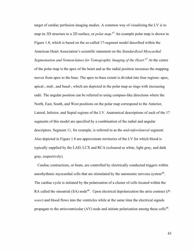
43

target of cardiac perfusion imaging studies. A common way of visualizing the LV is to

map its 3D structure to a 2D surface, or polar map.47 An example polar map is shown in

Figure 1.8, which is based on the so-called 17-segment model described within the

American Heart Association’s scientific statement on the Standardized Myocardial

Segmentation and Nomenclature for Tomographic Imaging of the Heart.47 At the center

of the polar map is the apex of the heart and as the radial position increases the mapping

moves from apex to the base. The apex-to-base extent is divided into four regions: apex,

apical-, mid-, and basal-, which are depicted in the polar map as rings with increasing

radii. The angular position can be referred to using compass-like directions where the

North, East, South, and West positions on the polar map correspond to the Anterior,

Lateral, Inferior, and Septal regions of the LV. Anatomical descriptions of each of the 17

segments of this model are specified by a combination of the radial and angular

descriptors. Segment 11, for example, is referred to as the mid-inferolateral segment.

Also depicted in Figure 1.8 are approximate territories of the LV for which blood is

typically supplied by the LAD, LCX and RCA (coloured as white, light gray, and dark

gray, respectively).

Cardiac contractions, or beats, are controlled by electrically conducted triggers within

autorhythmic myocardial cells that are stimulated by the autonomic nervous system48.

The cardiac cycle is initiated by the polarization of a cluster of cells located within the

RA called the sinoatrial (SA) node46. Upon electrical depolarization the atria contract (P-

wave) and blood flows into the ventricles while at the same time the electrical signals

propagate to the atrioventricular (AV) node and initiate polarization among these cells48.

44

Figure 1.8 The American Heart Association 17-segment model provides a 2D polar map representation

of the left ventricle. The coronary artery territories are indicated with gray shading. The region

corresponding to the left-anterior descending (LAD), left-circumflex (LCX) and right coronary (RCA)

arteries are shown in white, light gray, and gray, respectively. The outer annulus (segments 1 – 6)

corresponds to the basal region, the middle annulus (segments 7 – 12) corresponds to mid region, the

inner annulus (segments 13 – 16) corresponds to the apical level of the LV, and the apex (segment 17) is

shown at the center.

The AV node is located in the interatrial septum and is connected to conductive tissues

which travel down the septum and split near the apex before extending upwards toward

the bases of the RV and LV.46 The polarization and subsequent depolarization of the AV

node is referred to as the QRS-wave on electro-cardiograms (ECG) and trigger ventricular

contraction.48 Ventricular relaxation and re-polarization is triggered the T-wave.48 A

schematic representation of the electrocardiographic signals is illustrated in Figure 1.9.

The periods of ventricular contraction and relaxation are referred to as systole and

diastole.

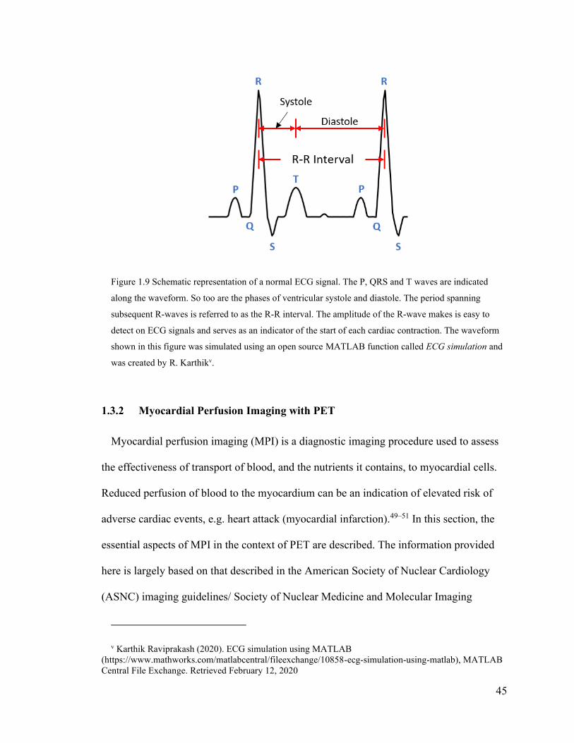
45

Figure 1.9 Schematic representation of a normal ECG signal. The P, QRS and T waves are indicated

along the waveform. So too are the phases of ventricular systole and diastole. The period spanning

subsequent R-waves is referred to as the R-R interval. The amplitude of the R-wave makes is easy to

detect on ECG signals and serves as an indicator of the start of each cardiac contraction. The waveform

shown in this figure was simulated using an open source MATLAB function called ECG simulation and

was created by R. Karthikv.

1.3.2 Myocardial Perfusion Imaging with PET

Myocardial perfusion imaging (MPI) is a diagnostic imaging procedure used to assess

the effectiveness of transport of blood, and the nutrients it contains, to myocardial cells.

Reduced perfusion of blood to the myocardium can be an indication of elevated risk of

adverse cardiac events, e.g. heart attack (myocardial infarction).49–51 In this section, the

essential aspects of MPI in the context of PET are described. The information provided

here is largely based on that described in the American Society of Nuclear Cardiology

(ASNC) imaging guidelines/ Society of Nuclear Medicine and Molecular Imaging

v Karthik Raviprakash (2020). ECG simulation using MATLAB

(https://www.mathworks.com/matlabcentral/fileexchange/10858-ecg-simulation-using-matlab), MATLAB

Central File Exchange. Retrieved February 12, 2020

46

(SNMMI) procedure standard for positron emission tomography (PET) nuclear

cardiology procedure52. Due to the extent to which this section relies on that report, it will

not be explicitly cited throughout. Additional resources have also been used and are cited

explicitly.

The goal of MPI is the detection of significant occlusion of coronary arteries that

supply blood the myocardium, otherwise known as ischemic Coronary Artery Disease

(CAD). Assessment of perfusion can help inform physicians of the best approaches for

managing patients with known or suspected CAD. MPI is typically conducted twice for a

single study; each corresponds to one of two physiologic conditions: rest or stress. Rest

and stress states are distinguished by the flow rate of blood: a resting state corresponds to

baseline blood flow rates and stress (or hyperemia) corresponds to elevated blood flow

rates. Stress can be induced in patients through exercise or with the use of pharmacologic

vasodilators agents that simulate exercise.

Normal perfusion during stress imaging is associated with the absence of significant

CAD, whereas reduced perfusion during stress is associated with ischemic CAD and/or

prior infarction. In the event that perfusion is abnormally reduced at stress but not at rest,

the ischemia is considered to be reversible, stress-induced ischemia. If perfusion defects

are matched between stress and rest, the defect is not reversible and is associated with

injury to the myocardium from prior infarct. Perfusion defects can exist regionally, or

globally within the myocardium depending the number of coronary arteries that exhibit

ischemia, e.g. single- versus multi-vessel CAD. The tracers used in MPI accumulate in

the myocardium in proportion to the blood flow to the region and integrity of the muscle

cells (myocytes). The activity shown on an uptake image also contains that of the tracer

47

concentration which is still in the blood and has not been taken up by the myocytes.53 As

defects are assessed based on the relative reduction in uptake compared to the maximum

uptake region (reference), global reduction in perfusion may appear to be normal. This

effect may be observed in the case of triple-vessel CAD, in which case standard MPI has

been shown to have an increase in false-negative test results. Likewise, global perfusion

reduction can result from disease of microvasculature, as is common in uncontrolled

diabetes.54,55 Determination of the absolute myocardial blood flow (MBF), as opposed to

relative perfusion, has been shown to improve the sensitivity of detection of CAD for

patients with globally reduced perfusion.56,57 MBF is a measure of the specific flow rate

of blood transiting through myocardial tissue in units of volume of blood per unit time

per gram of tissue (mL/min/g)58. Calculation of MBF necessitates dynamic imaging

procedures wherein the activity within regions of interest in myocardium can be sampled

as a function of time. Kinetic modelling of the radiotracer can then be performed to

estimate. This process will be described in greater detail in Section 1.3.3.

Perfusion data can be assessed qualitatively and/or semi-quantitatively to characterize

the defect(s). The following represent qualitative descriptors. The location indicates the

anatomical region of the myocardium in which a defect was observed. Due to the

association of segments of the myocardium with specific coronary arteries, location

information can provide insight as to the arteries involved with ischemic perfusion

defects. The extent of a perfusion defect corresponds to its relative proportion of the

myocardium size. Low, medium and large extents are associated with 5-10%, 10-20%,

and >20% of myocardium, respectively. The extent can also be described by the number

of left-ventricular segments that exhibit reduced perfusion.

48

Semi-quantitative assessments can be made as summed stress (SSS), summed rest

(SRS), and summed differences (SDS) scores. These measures are based on a 5-point

scale that stratify severity of perfusion defects within each of the 17 segments of the

myocardium. The point values range from 0 to 4, and correspond no defect, mildly

reduced, moderately reduced, severely reduced, and absent of activity, respectively. The

SSS and SRS correspond to the sum of the values among all 17 segments from the stress

and rest images, respectively. The SDS is the sum of the segmental differences between

stress and rest scores across (stress – rest). These scores can simultaneously assess both

severity and extent of perfusion defects. SSS scores in the ranges of 0-3, 4-7, and > 8,

correspond to normal, mildly abnormal, and moderately to severely abnormal,

respectively.

When quantitative MBF is performed, myocardial flow reserve (MFR) can also be

reported. MFR is determined as the ratio of MBF at stress to that at rest, indicating the

ability of blood supply to increase to meet cardiac demand with exercise. Lower limits on

normal stress MBF values, which range greatly among patients based on age, sex, and

presence of traditional cardiovascular risk factors, have been reported59 as 2 – 5 mL∙min-1

∙g-1. An MFR measurement greater than 2.3 corresponds to low risk of future adverse

cardiac events. An MFR less than 1.5 indicates significantly reduced flow and an increase

in risk of adverse cardiac events. Some discrepancy in these limits have been reported,

e.g. in a review paper by Juneau and colleagues60, limits of 2.0 and 1.7 for normal and

abnormal MFR were suggested. Stress MBF is often evaluated with MFR, as MFR alone

can be erroneously low if rest MBF, its denominator, is unusually high. This can occur in

patients with hypertension, for example.

49

The four most relevant perfusion tracers are 82Rb, 13N-ammonia, 15O-water, and 18F-

Flurpiridaz. In North America, PET MPI is largely restricted to the use of 82Rb and 13N-

ammonia, whereas 15O-water is also used in Europe and Japan.60 18F-Fluripiridaz61,

however, is currently the topic of a Phase III clinical trial in the Unites States.62–64

Several important properties like half-life, production method, kinetic behaviour,

extraction fraction, retention fraction, and effective dose per scan are summarized for

each of these tracers in Table 1.3.

The half-life of a radiotracer has a significant impact on how it can be used clinically.

82Rb, 13N-ammonia, and 15O-water, are relatively short-lived radiotracers; their half-lives

range from approximately 1 to 10 minutes, which necessitates rapid access for clinical

use. 13N-ammonia and 15O-water are produced using cyclotron accelerators that must be

located at the clinic. 15O production has been reported using the 15N(p,n) reaction65 and

13N has commonly been produced via the 16O(p,α) reaction.66 Note here that p, n and α in

these reaction formulae represent protons, neutrons and alpha particles, respectively.

82Rb, however, is produced using a 82Sr/82Rb (decay via electron capture) generator67 and

can be eluted approximately every 10 minutes as the 82Rb activity reaches secular

equilibrium with its parent isotope. 18F-based tracers must also be produced using

cyclotrons (e.g. via the 18O(p,n) reaction68) but its nearly 2 hours half-life allows it to be

transported from a production facility to the clinic. The half-lives are also associated with

radiation doses committed to the patients. Short-lived tracers generally lead to smaller

whole-body effective doses than longer-lived tracers. A typical PET MPI acquisition may

lead to effective doses in the range of 1 – 4 mSv. In contrast, SPECT tracers which have

50

99mTc as their radionuclide (which has half-life of 6 hours) lead to effective doses in

excess of 5 mSv59 or nearly as high as 10 mSv.69

The energy spectrum of the emitted positron affects its range within human tissue. Of

the four tracers listed in Table 1.3, 82Rb has the largest mean positron range. Increased

positron range has adverse effects on the spatial resolution of the images as the positron

may travel up to several millimeters away from its point of decay before annihilating with

an electron in tissue. Positron range thus imposes limits on the precision with which the

position of tracer can be estimated within the body.

The biological properties of the tracers also dictate how they can be used clinically. A

favourable tracer quality in the context of MPI is a specific biodistribution to the

myocardium which leads to enhanced contrast with non-target tissues (e.g. blood, lungs

and liver).59 Additionally, high retention of the tracer in the myocardium also makes

visualizing the myocardium more effective as the tracer distribution is stable for longer

periods of time.69 If MBF is being quantified, the rate of tracer extraction from the blood

into the target tissue is an important factor. When tracer extraction fraction is high,

measurements of MBF demonstrate less intra-patient variability as seen in repeated

imaging procedures (or test-retest measurements).69 Of the tracers listed in Table 1.3,

only 15O-water is not suitable for MPI as its retention fraction within the myocardium is

effectively zero. This is associated with the passive bi-directional diffusion of water

across the myocyte membrane59 which does not create stable uptake within the

myocardium. For the same reason, though, the extraction fraction for water is unity,

which means it is an ideal tracer for MBF quantification. The remaining perfusion tracers

have non-zero retention fraction and thus permit high quality visualization of uptake

51

within the myocardium. They also exhibit extraction fractions that are less than unity, and

thus necessitate the use of flow-dependent extraction-corrections functions to determine

MBF. 13N-ammonia and 18F-Flurpiridaz have extraction fractions that are relatively high

compared to 82Rb and are expected to provide higher precision estimates of MBF.59

Nevertheless, accurate MBF estimations has been reported for each of these tracers.70–73

Table 1.3 Physical and practical characteristics of commonly used PET radiotracers for MPI imaging.

The references associated with each characteristic are indicated after their names in the first column.

82Rb 13N-Ammonia 15O-Water 18F-Flurpiridaz

Half-life [min]60 1.3 10 1.9 110

Mean Positron Range in

Tissue60 [mm]

2.6 0.6 1.0 0.2

Production60 Generator On-site Cyclotron On-site Cyclotron Regional Cyclotron

Extraction Fraction69

(Stress - Rest)

0.40-0.70 0.95-0.99 1.00 > 0.9†

Retention Fraction69

(Stress - Rest)

0.30-0.70 0.50-0.90 0.00 0.6-0.9†

Effective Dose59 [mSv] 3‡ 1 0.4 4 † These extraction and retention fractions for 18F-Flurpiridaz were collected from Juneau and colleagues, unlike the

other values provided. ‡ Note that effective dose in the range of 1-2 mSv have been reported which include rest and stress acquisitions74.

1.3.3 Kinetic Tracer Modelling and Estimate of Absolute Myocardial Blood Flow

The use of kinetic modelling in the estimation of absolute MBF was alluded to in the

previous section. A description of kinetic modelling is provided here in the context of

MBF estimation. A PET image is a discretized representation of the activity

concentration within the body but the signal obtained for a given region of interest, or

even in a single voxel, represents a superposition of the contributions the tracer

concentrations in the constituent tissues contained within the image sampled region of

interest (ROI), or voxel. Moreover, these individual contributions are generally integrated

over the duration of the acquisition used to produce the image. Such an image is capable

52

of only spatial information of the tracer distribution within the body and provides limited

information regarding the dynamics of the tracer within specific tissues. The purpose of

kinetic modelling (KM) is to address such limitations; KM can be used to disentangle the

signal contributions of the unique physiologic constituents within a region that is being

sampled.53 More specifically, the kinetic model provides a relationship with which the

blood flow within myocardial tissue may be inferred from a dynamic series of activity

measurements taken from arterial blood and myocardial tissue.

Kinetic models are based upon coupled differential equations that relate the dynamics

of tracer molecules into and out of tissues that are relevant to the imaging target. The

individual constituents are referred to as compartments. Absolute blood flow can be

modelled using a two-compartment model (blood and perfused tissue), which is also

commonly referred to as a one-tissue-compartment model.75 A schematic representation

of this is provided in Figure 1.10(A). In this model the only tissue compartment is that of

the myocardial tissue to which arterial blood perfuses from the adjacent capillary or

capillary bed. The tracer concentration of the arterial blood, which serves as the input to

the kinetic model, and myocardial tissue as a function of time are denoted as Ca(t), and

Ct(t), respectively. The tracer influx and efflux rates are denoted as K1 and k2,

respectively. While the relationship will be shown explicitly in the following, it is worth

noting here that K1 is closely related to MBF and shares the same units. The net tracer

flux across the capillary wall, 𝑑𝐶𝑡(𝑡) 𝑑𝑡⁄ , is the difference between flux into and out of

the tissue compartment as shown in Eq. 0.16.53 This first order differential equation has

the solution for Ct(t), shown in Eq. 0.17,75 where the symbol ⨂ denotes a 1D convolution

operation.

53

𝑑𝐶𝑡(𝑡)

𝑑𝑡= 𝐾1𝐶𝑎(𝑡) − 𝑘2𝐶𝑡(𝑡)

Eq. 0.16

𝐶𝑡(𝑡) = 𝐾1𝐶𝑎(𝑡)⨂𝑒−𝑘2𝑡 Eq. 0.17

This model could be extended to a two-tissue-compartment model where the tissue is

further distinguished as the combination of myocytes and extracellular space, as shown in

Figure 1.10(B), but the additional parameters are not necessary for accurate MBF

estimation.67

Figure 1.10 One- (A) and Two-Tissue-Compartment (B) model representations of blood flow within the

myocardium. In both cases, capillary (Blood) regions and myocardial tissue are coloured as white and

gray, respectively. Black arrows indicate the directions of tracer flux across compartmental boundaries,

each of which is labelled with its respective rate constant. In the Two-Compartment model the

myocardial tissue region is divided into two more specific compartments which are the myocytes and the

extracellular space.

MBF estimation is the process of estimating the kinetic model parameters from a series

of measurements of the arterial input function and the myocardial tracer concentration.

The measurements are derived from a dynamic image reconstruction of the perfusion

study which begins with tracer injection and continues for a duration long enough to

observe tracer equilibrium. For 82Rb studies, dynamic acquisition with durations of 2 to 6

minutes have been reported.67

54

In practice, the kinetic model must be modified to account for the fact that a single

voxel of a PET image contains many capillaries and myocytes and the resultant signal

comes from the combination of these. The myocardial tracer concentration, which

contains blood and tissue, can be denoted as 𝐶𝑚(𝑡) and is the weighted sum of the arterial

blood and tissue tracer concentrations.67 The weights correspond to the fraction of the

volume being sampled that each component occupies. The fractional blood volume and

tissue volume are denoted as fa and ft, respectively. If we assume that the volume being

sampled is strictly composed of these two components then ft equates to 1 minus fa, and

we can reduce the complexity of our model by one free parameter. The estimated

myocardium tracer concentration ��𝑚(𝑡) is defined in Eq. 0.18. If we substitute the tracer

concentration of the tissue, defined previously, then our model takes on the form shown

in Eq. 0.19.

��𝑚(𝑡) = 𝑓𝑎𝐶𝑎(𝑡) + (1 − 𝑓𝑎)𝐶𝑡(𝑡)

Eq. 0.18

��𝑚(𝑡) = 𝑓𝑎𝐶𝑎(𝑡) + (1 − 𝑓𝑎)𝐾1𝐶𝑎(𝑡)⨂𝑒−𝑘2𝑡 Eq. 0.19

Both fa and ft are also interpreted as correction factors for the partial volume effect that

is associated with the limited spatial resolution of the imaging system which leads to

activity spilling into or out of a region of interest.53 The last amendment to this kinetic

model formula is the parameterization of K1 as a function of the myocardial blood flow,

MBF. This is necessary for tracers that do not exhibit an ideal first-pass extraction

fraction. The Renkin-Crone permeability model is commonly employed to derive the

functional form of K1.53 In this model K1 is equal to MBF multiplied by the first-pass

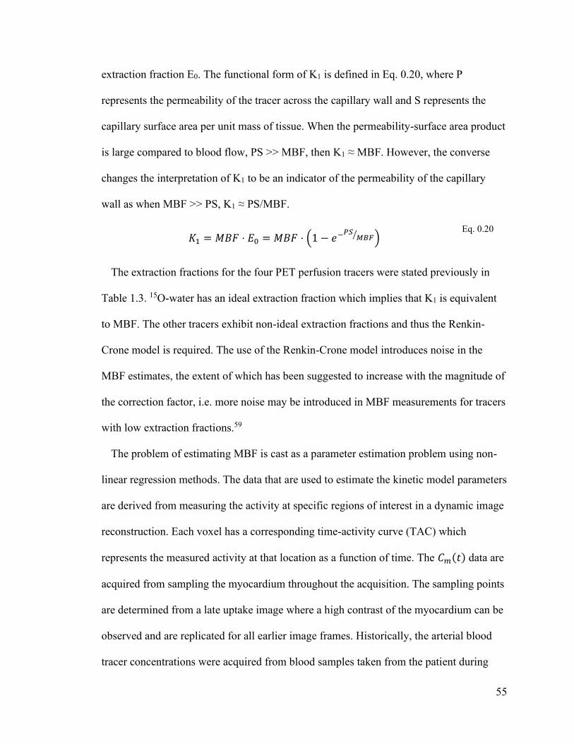
55

extraction fraction E0. The functional form of K1 is defined in Eq. 0.20, where P

represents the permeability of the tracer across the capillary wall and S represents the

capillary surface area per unit mass of tissue. When the permeability-surface area product

is large compared to blood flow, PS >> MBF, then K1 ≈ MBF. However, the converse

changes the interpretation of K1 to be an indicator of the permeability of the capillary

wall as when MBF >> PS, K1 ≈ PS/MBF.

𝐾1 = 𝑀𝐵𝐹 ⋅ 𝐸0 = 𝑀𝐵𝐹 ⋅ (1 − 𝑒−𝑃𝑆

𝑀𝐵𝐹⁄ ) Eq. 0.20

The extraction fractions for the four PET perfusion tracers were stated previously in

Table 1.3. 15O-water has an ideal extraction fraction which implies that K1 is equivalent

to MBF. The other tracers exhibit non-ideal extraction fractions and thus the Renkin-

Crone model is required. The use of the Renkin-Crone model introduces noise in the

MBF estimates, the extent of which has been suggested to increase with the magnitude of

the correction factor, i.e. more noise may be introduced in MBF measurements for tracers

with low extraction fractions.59

The problem of estimating MBF is cast as a parameter estimation problem using non-

linear regression methods. The data that are used to estimate the kinetic model parameters

are derived from measuring the activity at specific regions of interest in a dynamic image

reconstruction. Each voxel has a corresponding time-activity curve (TAC) which

represents the measured activity at that location as a function of time. The 𝐶𝑚(𝑡) data are

acquired from sampling the myocardium throughout the acquisition. The sampling points

are determined from a late uptake image where a high contrast of the myocardium can be

observed and are replicated for all earlier image frames. Historically, the arterial blood

tracer concentrations were acquired from blood samples taken from the patient during

56

imaging.53 However, sampling methods have also been established for image-based

measurements where a blood ROI is defined in the cavity of the left-ventricle or left-

atrium.52 Additionally, TACs can be derived from large regions-of-interest, segments of

LV myocardium, for example, or the individual voxels therein. Figure 1.11 provides an

example time-activity curve and LV polar map of blood flow from a clinical acquisition.

Figure 1.11(A) shows the measured and modelled TAC data for an example study. The

inputs to the one-tissue kinetic model described in Eq. 0.19, i.e. the measured blood pool

𝐶𝑎(𝑡) and myocardium 𝐶𝑚(𝑡) activities, are shown by the red line and blue dots,

respectively. The modelled myocardium ��𝑚(𝑡) and modelled tissue 𝐶𝑡(𝑡) activities,

related as shown in Eq. 0.18, are indicated by the dashed blue and cyan lines,

respectively. Figure 1.11(B) shows a polar map of the flow measurements within each of

the sampled LV voxels in units of mL/min/g.

Figure 1.11 Example kinetic modelling data from a clinical dataset. The time-activity curve (A) data are

shown for the measured blood pool (red), measured myocardium (blue dots), the modelled activity of the

myocardium (blue line), and modelled tissue (cyan) activity. The blood pool data have been averaged

over a volume of interest in the LV cavity and the myocardium data shown correspond to an average

across the entire LV. The polar map (B) depicts the estimated blood flow values in each of the voxels

sampled within the myocardium. The mean ± SD flow value for this case is also indicated.

57

Apart from the previously mentioned cardiac spillover effects, which are associated

with the partial volume effect, cardiac motion, and blood volume75, there are several

factors that can affect the precision of MBF estimation. Examples are CT attenuation

correction (AC) misalignment, extra-cardiac spillover, patient motion.76 CTAC artifacts

are most notable at the interface of the antero-lateral wall of the LV with left lung due to

the sharp gradient in the attenuation factors at this location, although careful registration

of the CT and PET images can largely reduce these artifacts67. Extracardiac spillover

corresponds to the contamination of activity measurements within the myocardium

ROI(s) from tissues that exhibit high uptake outside of the heart. In 13N-ammonia

perfusion studies late uptake in the left lung can lead to these effects in the lateral wall,

and in 82Rb studies stomach wall uptake can potentially interfere with measurements in

the infero-lateral segment.67

The effects of patient motion are the chief concerns of this thesis. Patient motion can

lead to CTAC misalignment artifacts as well as blurring in the PET images. Furthermore,

patient motion can lead to incorrect spatial sampling of the arterial blood or tissue

ROIs.77 A review of patient motion effects and compensation strategies is the topic of

Chapter 2.

1.4 Thesis Summary

The work described in this thesis was aimed at applying a data-driven motion tracking

technique to clinical cardiac PET/CT perfusion imaging studies to compensate for the

degrading effects of patient motion. Motion of the heart due to respiration as well as

whole-body motion are two separate problems that were considered. The primary

approach to motion compensation was based on tracking the motion of small radioactive

58

markers placed on patients during imaging. Calculations of the marker motion directly

from the raw list-mode data provided information that was used to infer the respiratory

patterns of patients or whole-body displacements and subsequently perform various types

of motion compensation. To evaluate the performance of the motion compensation

methods involving the use radioactive markers other approaches were also employed. A

commercial camera system was used to monitor patient respiratory patterns and a

previously developed data-driven motion tracking algorithm was implemented to address

whole-body motion.

59

Chapter 2 Patient Motion Tracking and Compensation

2.1 Patient Motions: Respiratory, Cardiac and Body

The problem of patient motion compensation is multi-faceted as there are various

forms of patient motion for which various solutions have been proposed. Head motion in

the context of brain PET imaging studies is effectively a rigid body problem as the brain

remains fixed within the structure of the skull.78 As a result, motion compensation

strategies that are effective in this application are not necessarily so for others. In the

thorax motion exists which can be associated with cardiac contraction, respiratory

displacements of the chest wall and the diaphragm, peristaltic motion, voluntary or

involuntary body motion79 as well as ‘cardiac creep’77 – a gradual repositioning of the

heart that may be observed during imaging as a patient’s breathing pattern returns to a

resting state following the induction of stress by treadmill exercise . For this work, the

primary concern is associated with cardio-respiratory, i.e. motion of the heart due to

respiration, and body motion, both of which represent non-rigid forms of motion.

Motion of the heart due to respiration was well documented in a study by McLeish and

colleagues80 where magnetic resonance imaging (MRI) was performed while patients and

healthy volunteers held their breath at various respiratory amplitudes ranging from full

inspiration to full expiration. They acquired data for approximately 30 seconds for each

breath-hold and performed rigid (translation and rotation) and non-rigid image

registrations on the resulting images to model the motion of the heart. With respect to

rigid motion of the heart during respiration they reported that motion along the superior-

inferior axis of the patient was dominant with a mean displacement of 12.4 mm compared

to 4.3 mm and 2.0 mm for motion along the anterior-posterior and right-left direction.

60

More qualitatively, as people inhale their hearts move toward their feet, their chest wall,

and slightly to the right. Rotations were more difficult to compare as the center of

rotations differed among subjects, however, while considering both translations and

rotations some points on the heart were displaced up to 30 mm between full inspiration

and expiration. In regard to non-rigid motion of the heart, there was also great inter-

subject variability – to such an extent that some exhibited no effective non-rigid cardiac

motion due to respiration. Some qualitative findings indicated that deformations were

generally greater at the apex compared to the base of the heart. The magnitude of

deformation tended to correlate with motion of the diaphragm, and non-rigid motion was

weakly correlated with the magnitude of rigid motion.

Body motion is more difficult to define than that of respiratory or cardiac motions. The

term body motion is vague and is often used to describe generally voluntary or

involuntary sources of motion like a deep cough or efforts exerted by a patient to re-

position themselves when in discomfort.77 Body motion is frequently modelled using

only translational descriptors which is certainly an oversimplification but also one that

has been demonstrated to be beneficial in regards to improving image quality and

quantification.81 In regard to cardiac perfusion PET studies several groups have published

reports on the prevalence, magnitude, and time of occurrence of rigid patient motion.

Hunter and colleagues82 reported that body motion with magnitudes ranging from 5 mm

to more than 10 mm was identified in 62% of cases among a cohort of 236 patients who

underwent 82Rb dynamic imaging aimed at measuring absolute myocardial blood flow.

They also reported that motion did not appear to be more frequent for any particular time

point during the 8-minute acquisitions. From most to least prevalent, they found that

61

motion prevalence was ordered as follows: the superior-inferior, anterior-posterior and

right-left axes. Among these, patients tended to move superiorly, posteriorly and equally

left and right. A similar study by Lee and colleagues83 examined body motion among 225

patients that underwent 82Rb myocardial perfusion imaging studies. They reported a time-

dependent motion prevalence noting that motion was found more frequently in the early

time frames when the tracer had not yet perfused into cardiac tissue particularly during

stress acquisitions. During stress acquisitions motion occurred more frequently toward

the inferior and septal (approximately to the right) directions. During rest, however,

motion in the inferior direction was predominant.

The long acquisition times associated with PET imaging make them more susceptible

to artifacts84 from all forms of motion that have just been described. The effect of patient

motion is largely that of inaccurate tracer distribution estimation due to a loss in spatial

resolution as well as mis-alignment with PET emission data and corresponding

attenuation correction map.85 When the motion extent is relatively large compared to the

spatial resolution of the scanner the effects become more severe which can potentially

lead to degradation in image quality which affects the interpretation of the images and,

possibly, misdiagnosis of the patient.84 Moreover, as PET systems continue to advance

with respect to hardware and reconstruction techniques the spatial resolution will

continue to improve thus leading to greater influence of patient motion on image

quality.84

Kortelainen and colleagues86 performed SPECT/CT acquisitions of a moveable cardiac

phantom wherein respiratory motion was simulated with varying magnitudes. They

demonstrated the perfusion defects became less pronounced in the presence of respiratory

62

motion compared to a motion-free acquisition. Additionally, the effects of motion were

predominant in the anterior and inferior walls of the cardiac phantom. In another study by

the same group, dual cardiac-respiratory gating was performed to assess the effect of

these forms of motion on function MPI measurements like LV volume, wall motion and

thickening.87 They demonstrated that dual gating for cardiac and respiratory motion

compensation led to small, but significant, increases in LV volume, and reductions in

wall thickening throughout the cardiac contraction. They did not, however, demonstrate

significant changes in relative perfusion measurements. It is important to note that both of

these studies were performed using SPECT/CT acquisitions which generally have spatial

resolution that is poorer than that of PET/CT. While trying to apply these measurements

to PET MPI, it is not unreasonable to expect that these effects could become more

pronounced.

For dynamic cardiac acquisition where absolute blood flow quantification is being

performed patient motion can affect not only image quality, as described for MPI, but

also the dynamic activity sampling within the blood pool and the myocardium.85

Incorrect sampling due to patient motion often presents itself in the time-activity curves

and manifests as discontinuities or spikes along the measured curves.77 In a small clinical

sample of seven patients, Yu and colleagues demonstrated that respiratory motion

correction led to substantial increases in MBF and CFR, e.g. mean increase of 15% and

19%, respectively. The increases tended to be larger when motion was more severe. In a

study by Hunter and colleagues82 that used an extensive computer simulated dataset

based on clinically observed translational motion, it was shown that errors in MBF as

high as 250% could be expected and as high as 500% in extreme cases.

63

2.2 Motion Tracking

To address the problem associated with patient motion many researchers have proposed

methods to compensate or correct for patient motion. Motion compensation may be

achieved through patient coaching and/or immobilization. This framework involves

communicating the importance of remaining motion-less to the patient, providing them

with training or explanations of the methods/devices that will be used to immobilize them

or minimize motion, as well as coaching during imaging. Immobilization methods are

largely applied within the domain of oncologic PET/CT studies used for radiation therapy

treatment planning88, but patient coaching or breath-hold techniques are more generally

applicable to PET studies covering the thorax, e.g. cardiac PET/CT. A discussion of these

methods is provided in Section 2.3.1.

Alternatively, there are also motion compensation or correction approaches that are

predicated on the use of a model of the patient’s motion, that do not require

immobilization and are less dependent on patient compliance with training or coaching.

To attain such motion information some sort of motion tracking system is needed. Two

general categories exist with which different tracking methods can be distinguished:

hardware and data-driven methods. The hallmark of the former category is the use of

some ancillary device that is used in addition to the medical imaging system that can

track a patient’s movement. The specific device used often depends on the type of motion

that is being tracked, but some common hardware systems consist of optical cameras

which track fiducial markers placed on the patient or non-visual systems that monitor

physiologic functions of the patient like respiration or electrocardiographic signals. A

brief review of some common hardware-based motion tracking systems is provided in

64

Section 2.2.1. Data-driven methods, however, seek to perform the same tracking tasks

without the use of ancillary devices. In particular, data produced by the imaging device

itself are used to generate information about a patient’s movement. The signal of a PET

scanner comes from the coincident detection of annihilation photons which are initially

collected in a simple list, sorted into emission sinograms, and then reconstructed into

tomographic images; various data-driven tracking methods have attempted to measure

patient motion using each of the data forms. The elegance of the data-driven methods

stems from their use of data that already exist without the need for additional, and often

expensive, equipment to track patient motion. The corollary of which is that patient setup

and preparation becomes more efficient which can be beneficial for patient comfort as

well as for the operation of the PET clinic. While these characteristics have significant

potential benefit, data-driven tracking methods are not well established in clinical use

compared to their hardware-based alternatives which are more established. While data-

driven methods remain largely in the domain of research89, several major PET scanner

vendors have now also begun offering commercial data-driven solutions for motion

trackingvi and indeed it will be interesting to see if their use becomes more commonly

adopted. A brief overview of various data-driven motion tracking methods is also

provided in Section 2.2.2.

The bulk of the work presented in this thesis, however, is aimed at one particular

motion tracking algorithm which is, in a way, a hybrid technique of the two categories

just described. The positron emission tracking algorithm, or PeTrack, is a computational

vi Examples of commercially available data-driven motion correction solutions: MotionFree, GE

Healthcare; and OncoFreeze, Seimens Healthcare.

65

method designed to track the motion of point-source positron-emitting markers using the

list-mode coincidence data. This method was originally designed for applications in

radiation therapy90 but was extended for use during positron emission tomography.91,92

PeTrack will be described in the following section.

2.2.1 Hardware-Based Tracking

Earlier in this section, the concept of a hardware-based tracking system was introduced.

In this section, more details about their use and several common commercial examples

are provided. This list is not exhaustive, but they are included here primarily to provide

the reader with some scope of the available options.

In the context of PET imaging, hardware-based tracking systems monitor, either

directly or indirectly, physiologic processes like respiration or cardiac contraction for the

purpose of modifying the image acquisition or the reconstruction to compensate for

associated motion artifacts. They are largely external monitors that are placed on the

patient and do not require invasive methods such as interstitial insertion which is used in

some radiation therapy applications.93 A principal assumption of their use is that the

external signal correlates well with internal motion of the imaging target. When

designing such devices several aspects must be taken into consideration: the invasiveness

of the device, patient comfort and tolerability, adaptability for different patients, and the

ease of set-up and/or use by the operator.94 Additionally, a good tracking system should

respond quickly to variations of the signal, not introduce shifts in the baseline signal,

should have high signal-to-noise ratio, and must not produce artifacts in the acquired

image.94 These systems monitor physiologic signals of the patient either directly or

indirectly; the latter is much more common. With respect to respiratory monitoring

66

systems, a direct monitor would consist of measures of the flow of air into and out of the

lungs, whereas indirect monitors usually correspond to monitoring movement of the

external surface of the patient’s chest or abdomen. These systems generally track

respiratory motion at a frequency of 25 to 40 Hz and can respond quickly to human

breathing rhythms which have principal frequencies in the approximate range of 0.1 to

0.5 Hz. For applications in PET, these systems generate respiratory triggers that mark

specifics phases or amplitudes of the respiratory cycles. The respiratory triggers of

devices that can be integrated with the PET system can be included in the coincidence

event stream (list-mode data) and retrospectively used to gate the raw data according to

phase or amplitude. If the tracking system cannot be integrated with the PET system in

this way, the recorded signals can be processed retrospectively to allow a user to

reconstruct a respiratory-gated image series. Table 2.1 provides details of several

respiratory monitoring systems that have been used in respiratory-gated PET/CT studies.

The two most used respiratory monitoring devices are the Real-time Position

Management (RPM) system (Varian Medical Systems, Palo Alto, United States of

America) and the Respiratory Gating System AZ-733V (Anzai Medical, Tokyo, Japan).94

Details on these are included in the table below, but briefly, the RPM is an optical

tracking system which records the motion of a plastic block with reflective markers

placed on the patient’s chest or abdomen and the Anzai system is a belt-device worn by

patients that produces an electric signal that is correlated with pressure induced by its

expansion during respiration.

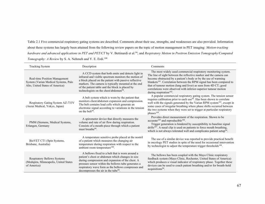
67

Table 2.1 Five commercial respiratory gating systems are described. Comments about their use, strengths, and weaknesses are also provided. Information

about these systems has largely been attained from the following review papers on the topic of motion management in PET imaging: Motion-tracking

hardware and advanced applications in PET and PET/CT by V. Bettinardi et al.94; and Respiratory Motion in Positron Emission Tomography/Computed

Tomography: A Review by S. A. Nehmeh and Y. E. Erdi.100

Tracking System Description Comments

Real-time Position Management

System (Varian Medical Systems, Palo

Alto, United States of America)

A CCD system that both emits and detects light in

infrared and visible spectrum monitors the motion of

a block placed on the patient with passive reflective

markers. The camera is typically mounted at the end

of the patient table and the block is placed by

technologists on the chest/abdomen94.

The most widely used commercial respiratory monitoring system.

The line of sight between the reflective marker and the camera can

become obstructed by a patient’s body or by the use of warming

blankets101. Correlation between the RPM signal has been compared to

that of tumour motion (lung and liver) as seen from 4D CT; good

correlations were observed with inferior-superior tumour motion

during respiration102.

Respiratory Gating System AZ-733V

(Anzai Medical, Yokyo, Japan)

A belt system which is worn by the patient that

monitors chest/abdomen expansion and compression.

The belt contains load cells which generate an

electronic signal according to variations in the tension

on the belt94.

A popular commercial respiratory gating system. The tension sensor

requires calibration prior to each use94. Has been shown to correlate

well with the signals generated by the Varian RPM system103, except in

some cases of irregular breathing where phase shifts occurred between

the two systems when they were set to trigger at particular respiratory

phases104.

PMM (Siemens, Medical Systems,

Erlangen, Germany

A spirometer device that directly measures the

volume and rate of air flow during respiration.

Consists of a mouth-piece through which a patient

must breathe94.

Provides direct measurement of the respiration. Shown to be

accurate105 and reproducible106.

Trigger generation is hindered by susceptibility to baseline signal

drifts107. A nasal clip is used on patients to force mouth breathing,

which is not always tolerated well and complicates patient setup94.

BioVET CT1 (Spin Systems,

Brisbane, Australia)

A temperature sensitive probe placed at the nostril

of a patient which measures the changing air

temperature during respiration with respect to the

ambient room temperature100.

The use of a similar device was reported to provide practical benefit

in oncology PET studies in spite of the need for occasional intervention

by technologist to adjust the temperature trigger thresholds108.

Respiratory Bellows Systems

(Medspira, Minneapolis, United States

of America)

A bellows fixed to a belt that is worn around a

patient’s chest or abdomen which changes in size

during compression and expansion of the chest. A

pressure sensor within the bellows tube generates a

respiratory wave form as the bellows compresses and

decompresses the air in the tube94.

The bellows has been coupled with the Mayo Clinic respiratory

feedback system (Mayo Clinic, Rochester, United States of America)

which produces a visual indicator of respiratory phase. Together these

devices can be used to coach patient breathing and/or for breath-hold

acquisitions94.

68

Other optical tracking systems have been designed to monitor (in)voluntary rigid

patient motion. Two commonly used systems during neurological PET studies are the

Polaris95 and Vicra96 tracking devices (Northern Digital, Waterloo, Ontario, Canada).

These devices track the rigid (rotations and translation) motion of passive reflective

markers that are fixed to a support structure that is mounted on a patient’s head during an

imaging procedure.95

2.2.2 Data-Driven Tracking

One of the earliest, and perhaps most intuitive, methods of tracking patient motion

using data derived from the PET scanner was based on multiple acquisition frame (MAF)

image reconstructions. Within this framework, many images would be reconstructed from

short time intervals of the acquisition from which the motion of the patient could be

inferred. The MAF approach was initially proposed by Picard and Thompson97, although

in their implementation the motion information was derived from an external optical

tracking system. Nevertheless, the MAF approach was later adapted for use in PET

motion tracking without an external tracking system. Feng et al.98, proposed a method of

extracting patient motion information from a time-series of tomographic SPECT or PET

images by identifying a generalized set of center-of-mass point within image volumes

and tracking their motion dynamically. Mukherjee et al.99 estimated patient motion

during brain PET studies via mono-modality image registration of short duration (5 s).

Using modern hybrid PET/MR scanners, simultaneous dynamic MR acquisitions have

been used to estimate high-resolution patient motion also with the use of image

69

registration techniques. This approach has been applied to estimate cardiac and

respiratory motions.109,110

A significant limitation of the MAF motion estimation approach is the computational

burden of reconstructing many images. To address this issue, others have implemented

data-driven motion estimation/tracking methods that rely, instead, on the raw emission

data acquired by the scanner. In the case of PET scanners, these data are typically stored

in three-dimensional sinograms. If the scanner has TOF capability, then the raw emission

data may instead be stored as a four-dimensional sinogram. This format of the data

includes all prompt coincidence detections which have not been corrected for losses due

to deadtime, detection efficiency, attenuation or decay of the radiotracer, yet many have

shown that raw emission data contains useful information from which patient motion can

be inferred.

Klein and Huesman111 demonstrated that the temporal fluctuations of the axial center-

of-mass of the emission data could be used to derive meaningful respiratory signals of

patients undergoing PET acquisitions with stable radiotracer distributions, e.g. 18F-FDG.

Others have identified sets of voxels in the 3D raw data space that exhibit large

magnitudes in the power spectra in the range of frequencies that correspond to respiratory

motion and then derived respiratory signals from the intensity fluctuations within this set

of voxel throughout the PET acquisition.112,113 Thielemans et al114 proposed the

application of principal-component analysis (PCA) on short frames of the raw emission

data to extract motion signals that correspond to cyclical motions.

The most basic form of the data acquired by PET scanner is the list-mode data, which

is simply a record of each prompt coincidence event detected by the scanner interspersed

70

with regular time-stamp events. The coincidence events contain indices of the crystal-pair

that detected the event from which the geometric information about the event, or LOR,

can be determined. Others have proposed tracking methods using list-mode data in which

no radioactive markers were used. The capability of storing list-mode data is relatively

new compared to the lifespan of PET systems, and so data-driven methods using this data

format are also relatively new. One of the earliest approaches was proposed by He et

al115, in which the coincidence count-histogram of the list-mode events over short time

frames was used to estimate a respiratory signal. This method, based on knowledge of the

geometric sensitivity profile of common PET scanners with a limited axial FOV,

assumed that respiratory motion would cause temporal fluctuations in the scanner count

rate as tissues with high radiotracer uptake move within regions of spatially variant

detection sensitivity. Others calculated the axial component of the trajectories of the

center-of-mass of LORs corresponding to regions-of-interest about the imaging targets,

e.g. the heart in cardiac PET acquisitions, over short time frames to derive respiratory

signals.116,117 Lastly, investigators at the Yale PET Center have developed centroid-of-

distribution tracking methods to estimate respiratory and whole-body (or bulk) patient

motion signals.118,119 In this approach, the geometric centroid of a set of LORs, either

associated with full scanner FOV or a region-of-interest, is tracked over short time

intervals to derive a 3D motion signal of the patient.

In addition to the data-driven approaches just mentioned, several other groups have

studied the use of tracking the motion of external radioactive fiducial markers with the

PET system. These methods constitute a hybrid approach between hardware and data-

driven methods in that the PET scanner is being used to produce the tracking signal, but

71

the signal is derived from an external radioactive source placed within the PET scanner’s

FOV. Interestingly, radioactive markers have been used in each of the data-driven

frameworks just described, i.e. image-based MAF motion tracking, motion tracking with

emission data, and also using list-mode data. Examples of MAF motion tracking are

found in the work of Naum et al.120 who used external markers to retrospectively track

patient motion in dynamic H215O cardiac blood flow studies and also Nazarparvar et al.121

who reconstructed 0.5 s duration frames during brain PET simulation studies to estimate

head motion during the acquisitions. Büther et al.122 reported their use of radioactive

marker motion tracking in short duration sinograms for respiratory gating during liver

and lung oncological PET studies. The PeTrack algorithm, proposed in this thesis, is an

example of a radioactive marker-tracking approach that operates on list-mode data which

has been applied to respiratory gating (see Chapter 3) and whole-body motion tracking

(see Chapter 4 and Chapter 5) in cardiac perfusion PET studies. The PeTrack algorithm

will be described in Section 2.4 along with a motivation for its use compared to these

alternative methods.

2.3 Compensation and Correction

2.3.1 Breath-hold Techniques and Patient Immobilization

Prior to the inclusion of motion tracking systems in the clinical environment, and

currently in busy clinics or those without resources to invest in additional motion-

tracking equipment, motion compensation is attempted by a combination of patient

training prior to imaging, patient coaching during imaging, and immobilization devices.

72

Even in the presence of motion compensation systems, educating patients on the

importance of remaining as motionless as possible during imaging is essential.

Breath-hold techniques are characterized by acquiring data during periods when the

patient is not breathing. As there are limits to the amount of time that a person can

comfortably hold their breath, multiple acquisitions are typically required during breath-

hold and are then summed to generate a final image from a sufficient number of counts.

Typically, the patient is instructed or coached to hold their breath at a specific respiratory

phase. Deep-inspiration breath-holds during PET acquisitions have been investigated

extensively100, particularly in the context of oncologic studies of the thorax where

respiratory motion can significantly reduce the apparent uptake of small lesions in the

lungs or liver.123 Breath-hold techniques have also been investigated in the context of

myocardial perfusion imaging124 but the clinical use has been marred by the potential for

extended imaging time, reduced throughput, patient discomfort, and, possibly, increased

radiation dose125. The specific breath-hold protocols vary in terms of the number of

acquisitions and duration of individual breath-holds, and breath-holds ranging from 20

seconds to as long as comfortably tolerated by patients have been reported.123,126,127

Mitsumoto and colleagues128 sought to investigate various protocols to determine the best

with respect to enhancing thoracic lesions uptake and recommended that at least three, 20

second, breath-hold acquisitions be used. Kini and colleagues129 have also found that the

methods used to coach patient-breathing also have an impact on the overall performance.

Coaching methods included a combination of audible prompts and visual feedback of the

patient’s real-time respiratory displacement.

73

Immobilization devices have also been proposed to control or suppress respiratory

and/or body motion during PET acquisitions.88 In the context of cardiac perfusion studies,

Ichikawa and colleagues130 investigated the use of an abdominal belt worn by patients to

suppress the extent of respiratory motion. They found that the belt system, which the

study participants reported as being well tolerated, significantly reduced the motion of the

heart due to respiration compared to free-breathing: 8 mm of motion compared to 12 mm,

respectively. They also showed that the belt aided in reducing the frequency of artifactual

reductions in tracer uptake associated with respiratory motion during free-breathing. A

pulsatile flow ventilation (PFV) system, not unlike a sleep apnea machine, was

investigated by Prior and colleagues131 in a cohort of four patients to immobilize patient

respiration while still providing constant oxygen supply and carbon dioxide extraction.

While breath-holds may be maintained for periods up to 30 seconds by most patients, the

PFV system was able to produce an apnea-like state among these patients for periods

greater than 8.5 minutes. The authors indicated that nearly 45 minutes was required for

patient preparation and device setup.

2.3.2 Respiratory and Cardiac Gating

For PET studies where the imaging targets are located in the thorax, cyclical

respiratory and cardiac motion are present that can lead to motion-induced artifacts.

Aside from the breath-hold and respiratory suppression techniques just described, motion

tracking systems can be employed to monitor patient respiration to provide a form of

motion compensation known as gating. Gating is a process by which acquisitions are

limited to particular phases (or amplitudes) of a cyclical physiological process. In regard

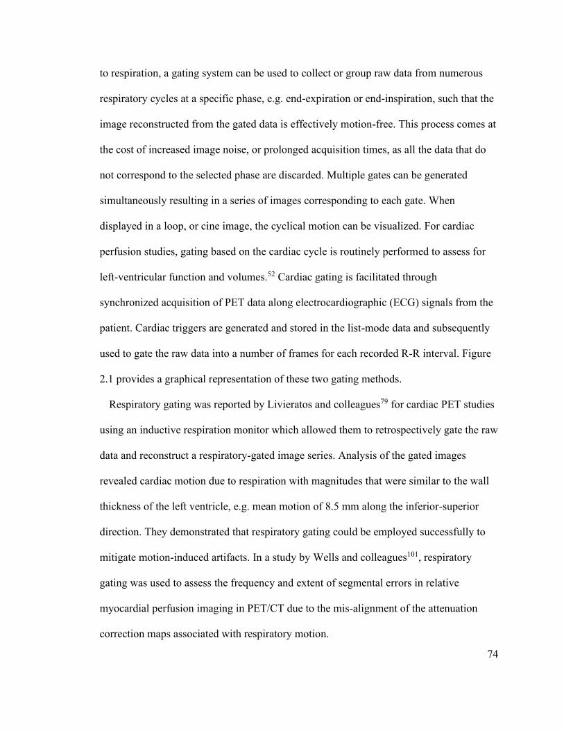
74

to respiration, a gating system can be used to collect or group raw data from numerous

respiratory cycles at a specific phase, e.g. end-expiration or end-inspiration, such that the

image reconstructed from the gated data is effectively motion-free. This process comes at

the cost of increased image noise, or prolonged acquisition times, as all the data that do

not correspond to the selected phase are discarded. Multiple gates can be generated

simultaneously resulting in a series of images corresponding to each gate. When

displayed in a loop, or cine image, the cyclical motion can be visualized. For cardiac

perfusion studies, gating based on the cardiac cycle is routinely performed to assess for

left-ventricular function and volumes.52 Cardiac gating is facilitated through

synchronized acquisition of PET data along electrocardiographic (ECG) signals from the

patient. Cardiac triggers are generated and stored in the list-mode data and subsequently

used to gate the raw data into a number of frames for each recorded R-R interval. Figure

2.1 provides a graphical representation of these two gating methods.

Respiratory gating was reported by Livieratos and colleagues79 for cardiac PET studies

using an inductive respiration monitor which allowed them to retrospectively gate the raw

data and reconstruct a respiratory-gated image series. Analysis of the gated images

revealed cardiac motion due to respiration with magnitudes that were similar to the wall

thickness of the left ventricle, e.g. mean motion of 8.5 mm along the inferior-superior

direction. They demonstrated that respiratory gating could be employed successfully to

mitigate motion-induced artifacts. In a study by Wells and colleagues101, respiratory

gating was used to assess the frequency and extent of segmental errors in relative

myocardial perfusion imaging in PET/CT due to the mis-alignment of the attenuation

correction maps associated with respiratory motion.

75

Figure 2.1 Schematic representation of the gating process. Triggers can be derived from physiologic

monitoring devices, e.g. ECG or respiratory monitoring systems, as well as based on pre-defined

dynamic time frames. In the dynamic acquisition the list-mode data from each reconstructed frame come

from contiguous blocks. In the ECG or respiratory gated acquisitions, the data corresponding to each

frame are sampled throughout the original data set in a repeating fashion corresponding to the

physiologic state of each frame. The ECG signal shown here was produced using an open-source

function by Kathrik Raviprakash (2020)vii.

The Varian RPM system was used to monitor respiratory motion. Within a cohort 190

patients, 310 scans acquired at rest or stress were initially evaluated. From these, nine

were exhibited significant motion and significant segmental perfusion differences

between the end-inspiration and end-expiration gates. The reconstructions for these 9

vii Kathrik Raviprakash (2020) ECG simulation using MATLAB,

http://www.mathworks.com/matlabcentral/fileexchange/10858-ecg-simulation-using-matlab, accessed

January 14, 2020.

76

scans were repeated with respiratory-phase matched attenuation correction. The

segmental perfusion errors were corrected in 8 of the 9 cases.

While cardiac gating is not generally performed for the purpose of motion

compensation, research on that topic is not uncommon, an example of which was

reported by Martinez-Möller and colleagues132 in a study where both cardiac and

respiratory gating were applied to generate images corresponding to end-diastole at

various respiratory phases. In their study they reported information about non-rigid

cardiac deformations that occurred due to respiratory motion alone, i.e. they showed that

greater motion was observed for the inferior LV wall compared to the anterior wall. In

another study by Germino and Carson75, cardiac gating was used to perform kinetic

modelling of myocardial blood flow in simulated and human (N = 1) 82Rb studies such

that both blood flow and cardiac function could be assessed simultaneously. Additionally,

respiratory motion compensation was also applied based on respiratory motion tracking

using the Anzai pressure belt system described previously (see Table 2.1).

2.3.3 Motion Correction

In a similar fashion to the data-driven motion tracking methods described previously,

motion correction has been employed before, during, and after the image reconstruction

process on different formats of available data. In this section an overview of the most

common classes of motion correction strategies are introduced.

One of the most common approaches to motion correction corresponds to the extension

of the multiple-acquisition frame (MAF) motion estimation approach described in

Section 2.2.2 where a final motion-corrected image is produced after averaging the set of

77

registered frames. An early example of this method was reported by Klein and

colleagues133 where a non-rigid image registration technique was employed to transform

a set of gated images to the reference gate and then sum the images. In their study they

tested their approach on a cardiac-gated PET study performed on a dog but only

attempted registration (and summation) of images corresponding to end-diastole and end-

systole. They reported qualitative improvements observed in the motion-corrected images

compared to summation without motion correction. A more recent study by Slomka and

colleagues134 reported the use of the MAF motion correction approach applied to dual-

gated cardiac perfusion PET studies. In their approach both respiratory and cardiac

motion triggers are inserted into the list-mode data and using these they separately

reconstructed cardiac or respiratory-gated images. From each gated series, cardiac and

respiratory motion are estimated independently using image registration techniques. The

two motion models were then combined to produce a single motion-corrected image.

They showed significant improvements in myocardial contrast and significant reductions

in image blur as measured by LV wall thicknesses.

Prior to image reconstruction the available data correspond to the list-mode or raw

projection (sinogram) data. Several groups have developed event-by-event motion

correction methods wherein individual LORs in the list-mode data are transformed to

account for the motion exhibited by a patient. One of the earlier examples of this

approach was studied by Bloomfield and colleagues95 in the context of neurological PET

studies. In their work, an optical motion tracking system was used to monitor 3D real-

time head motion, which was retrospectively used to transform individual LORs to

correspond to a reference position. Using data from a physical phantom and a single

78

patient acquisition promising results were shown. Most notably, while performing the

kinetic modelling on the patient data set, motion correction was shown to improve the

obvious motion-induced irregularities of the time-activity curves. Livieratos and

colleagues135 also applied rigid transformation to individual LORs using motion data

gleaned from image-registration of respiratory-gated images in cardiac PET studies. They

demonstrated improvements in the contrast recovery coefficient in phantom studies

where respiratory-like motion was simulated. In both of these approaches, care must be

taken after transforming LORs to account for the spatially variant changes in the scanner

detection efficiency as well as attenuation correction as transforming a given LOR results

in different trajectories through the patient’s body as well as crystal-pair end points.

Another approach is to incorporate motion data into the image reconstruction process

by extending the scanner system matrix to be four dimensional where the fourth

dimension is a temporal component that includes patient motion information. The

forward and back-projectors could be modified, for example, to have different photon

trajectories for specific frames or instances throughout the acquisition. Qiao and

colleagues136 demonstrated such an approach using numerical and physical phantom

simulation studies of respiratory-gated cardiac PET/CT studies. In their work they

assumed that 4D respiratory-gated CT images were available, from which a respiratory

motion-model could be established and applied to the gated PET data for respiratory

motion correction. They demonstrated image quality improvements like increased signal-

to-noise ratios and reduced bias when performing motion correction by modifying the

PET system matrix with measured motion data. Deriving motion information from 4D

CT data, however, is generally not desirable due to the increased radiation exposure137 to

79

patients compared a single, static, CT acquisition. Additionally, 4D CT acquisitions may

also lead to increased complexity of imaging protocols.101 It follows that these data are

often unavailable to generate patient-motion models.

Others have developed methods that extended the statistical likelihood model to

include transformation parameters, rigid or otherwise, such that joint estimation of the

motion parameters and the image occur during the reconstruction process. Jacobson and

Fessler138 proposed such an approach which was tested on numerical phantom studies.

They found that the joint estimation approach led to more accurate motion estimation but

did not improve lesion uptake when compared to post-reconstruction image registration

methods. More recently, Kalantari and colleagues139 developed a similar approach but

they reportedly used non-rigid image registrations to initialize motion models prior to the

joint image and motion estimation. They reported significant reduction in blurring of

lesions of various size and uptake using numerical phantom studies which included

respiratory motion.

One common drawback among these motion correction approaches is that they make

use of raw data that have already been gated and it follows that intra-gate motion may

exist for which they are not able to account. In some of the methods where motion

estimation was achieved from a system that is independent of the images, e.g. the optical

tracking system used by Bloomfield95 in the brain PET studies, this problem may be

obviated. Moreover, Klein et al133 reported that caution should be exercised when

estimating motion information from PET images as they are generally noisy and of low

spatial resolution and it follows that errors may propagate into the motion estimates.

80

2.4 Positron Emission Tracking (PeTrack)

2.4.1 The Tracking Algorithm

Before describing PeTrack it is helpful to review quickly the β+ decay process which

effectively terminates following the detection of the resulting annihilation photons.

Recall from Section 1.1.2 that following a β+ decay, the positron will travel some

distance in its surrounding medium before annihilating with an electron. The resulting

annihilation photons will then be emitted in an approximately collinear fashion (180º)

and be observed by a detection system which has some finite spatial resolution. Each of

these cascading processes influences one’s ability to determine the position from which

the decay originated. It follows that a model of the probability density function (PDF)

that describes this spatial distribution can be produced to help make inferences about the

position of the radioactive source based on detection of the annihilation photons. This is

the approach that was developed for PeTrack to track the motion of physically small

positron-emitting markers. The following description of the PeTrack algorithm is largely

based on work reported elsewhere. The basic tracking algorithm was originally described

by Xu and colleagues90 and then extended for use during PET by Chamberland and Xu.91

The PeTrack formalism is described in the following and is based upon the description of

these two sources.

An essential assumption of the PeTrack method was that the PDF can be modelled by a

Gaussian function with a mean value that corresponds the true marker position and a

standard deviation which results from the combined effects that limit the spatial

resolution of the detection system. Consider that in some span of time a set of 𝑁 lines-of-

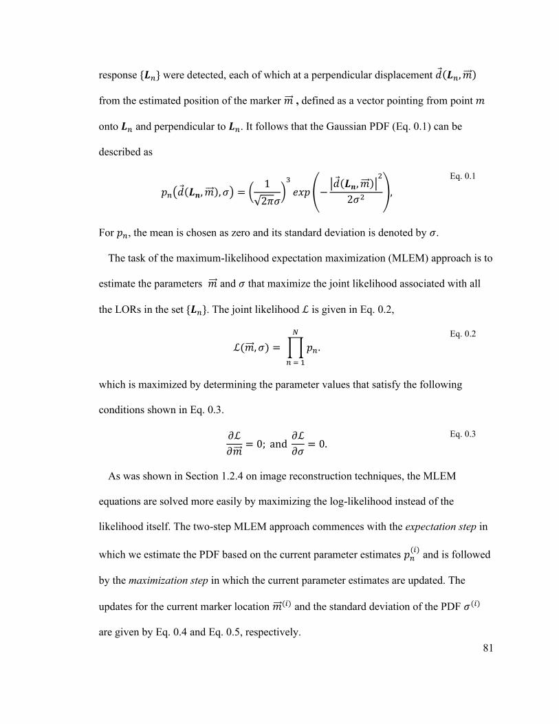
81

response {𝑳𝑛} were detected, each of which at a perpendicular displacement 𝑑(𝑳𝑛, ��)

from the estimated position of the marker �� , defined as a vector pointing from point 𝑚

onto 𝑳𝑛 and perpendicular to 𝑳𝑛. It follows that the Gaussian PDF (Eq. 0.1) can be

described as

𝑝𝑛(𝑑(𝑳𝒏, ��), 𝜎) = (1

√2𝜋𝜎)

3

𝑒𝑥𝑝 (−|𝑑(𝑳𝒏, ��)|

2

2𝜎2),

Eq. 0.1

For 𝑝𝑛, the mean is chosen as zero and its standard deviation is denoted by 𝜎.

The task of the maximum-likelihood expectation maximization (MLEM) approach is to

estimate the parameters �� and 𝜎 that maximize the joint likelihood associated with all

the LORs in the set {𝑳𝑛}. The joint likelihood ℒ is given in Eq. 0.2,

ℒ(��, 𝜎) = ∏ 𝑝𝑛

𝑁

𝑛 = 1

.

Eq. 0.2

which is maximized by determining the parameter values that satisfy the following

conditions shown in Eq. 0.3.

𝜕ℒ

𝜕��= 0; and

𝜕ℒ

𝜕𝜎= 0.

Eq. 0.3

As was shown in Section 1.2.4 on image reconstruction techniques, the MLEM

equations are solved more easily by maximizing the log-likelihood instead of the

likelihood itself. The two-step MLEM approach commences with the expectation step in

which we estimate the PDF based on the current parameter estimates 𝑝𝑛(𝑖)

and is followed

by the maximization step in which the current parameter estimates are updated. The

updates for the current marker location ��(𝑖) and the standard deviation of the PDF 𝜎(𝑖)

are given by Eq. 0.4 and Eq. 0.5, respectively.

82

��(𝑖+1) = ��(𝑖) + ��(𝑖)

Eq. 0.4

𝜎(𝑖+1) = √∑ 𝑝𝑛

(𝑖)|𝑑(𝑳𝒏, ��)|

2𝑁𝑛=1

∑ 𝑝𝑛(𝑖)𝑁

𝑛=1

Eq. 0.5

The position update contains the step vector ��(𝑖) which is computed as shown in Eq. 0.6.

��(𝑖) =

∑ 𝑝𝑛(𝑖)

𝑑(𝑳𝒏, ��)𝑁𝑛=1

∑ 𝑝𝑛(𝑖)𝑁

𝑛=1

Eq. 0.6

The initial estimate of the standard deviation is set to 5 mm. The initial estimate of the

marker position is more involved in the application of PeTrack to PET imaging and will

be described more carefully in Chapter 3. Convergence of the MLEM method was

defined as position updates that are smaller in magnitude than 0.05 mm.

The original PeTrack algorithm was extended for use during PET imaging by

Chamberland, deKemp, and Xu and is referred to as Adaptive Region of Interest

(ADROI) PeTrack.92 Note that the ADROI PeTrack algorithm will be referred to

hereafter as PeTrack. This modification included additional processing steps to overcome

challenges not incurred during radiation therapy: the separation of the positron-emission

signal of the fiducial markers from that of the radiotracer administered to the patient. To

address this issue, knowledge of the physical characteristics of the fiducial markers and

spatial distribution of the radiotracer have been exploited. The first step in the

background rejection is to generate a spherical region-of-interest with a radius of 30 mm

about the initial marker position. LORs with a perpendicular distance, |𝑑(𝑳𝑛, ��)|, greater

than 30 mm are excluded from the active set of LORs and thus are not included during

the iterative PeTrack method. The second step makes use of the time-of-flight delay of

83

each coincident event, assuming it is available, to impose further restrictions. As was

mentioned in Section 1.2.2.3, the TOF resolution of a PET camera is a measure of the

degree of precision with which the most likely annihilation (MLA) position can be

estimated along a given LOR. This knowledge was used such that LORs with MLA

position greater than 80 mm from the current marker position are excluded from further

processing. A third step is employed that excludes LORs with a perpendicular distance

that is less than a specific cut-off from the central axis of the PET scanner. This step is

useful as the marker is placed on the skin of a patient and physically cannot be closer to

the central scanner axis than the patient’s body size permits. In regard to the work

described in this thesis, the cut-off distance was estimated on a per-patient basis as a

fraction of the initial marker’s vertical (anterior-posterior) distance from the central axis,

i.e. 0.8 ∙ |��𝑦(0)

|. Lastly, the adaptive region-of-interest (ADROI) method was developed

which models the spatial distribution of the radiotracer near the marker to further

constrain the set of LORs that are used for tracking with PeTrack. It was previously

demonstrated that if the 3D probability density function (PDF) of 𝑑(𝑳𝑛, ��) could be

modelled as an isotropic Gaussian function with standard deviation 𝜎, then the distance

follows a 1D PDF shown in Eq. 0.7.92

𝑃𝐷𝐹(|𝑑(𝑳𝑛, ��)|) = 4𝜋|𝑑(𝑳𝑛, ��)|2

(1

√2𝜋𝜎)

3

exp (−|𝑑(𝑳𝑛, ��)|

2

2𝜎)

Eq. 0.7

Additionally, the local tracer background can be modelled as a linear function of

|𝑑(𝑳𝑛, ��)| which increases with increasing distance from the ROI centroid.92 The

background can be fit using simple linear regression and then subtracted from the

84

histogram. The ROI size is adapted by truncating the histogram up to the first histogram

bin in which the number of LORs is less than or equal to zero after background

subtraction. A schematic diagram of this fitting procedure is provided in Figure 2.2. In

the event the radius of the ROI become so small that fewer than 10 LORs are included, it

is expanded by a factor of 3 and the adaptive ROI fitting method is repeated. This entire

process is repeated for subsequent tracking instances, i.e. those of the following time

frames. Each subsequent tracking instances uses the final position of the previous run as

the new initial marker position estimate.

Figure 2.2 The adaptive region-of-interest procedure is exemplified in this figure which shows the

histogram of LORs with a perpendicular distance ‘r’ (denoted in this work as |𝑑(𝑳𝑛 , ��)|) from the

estimated marker position from a phantom acquisition. The columns with hashed lines indicate the

events following the initial ROI and TOF based rejection techniques. The solid black line represents a fit

of the combined marker PDF and linear background model. The marker PDF and linear background fits

are shown as the dotted and dashed lines, respectively. The solid gray bars indicate the events that

remain following subtraction of the linear background fit. In this example the ADROI size was set as 8

mm. This figure was used with permission from the work of Chamberland, deKemp and Xu.92

85

Currently, no parallelization acceleration techniques are employed during tracking with

PeTrack. It takes approximately 15 minutes to generate a 3D marker motion trace for a

typical 82Rb cardiac perfusion study (~108 LORs), on a PC workstation with an Intel Core

i7-6700 processor (3.40 GHz). Execution times tend to increase when convergence is

slow, e.g. if the marker signal is too weak compared to the background radiotracer

activity. In the event that a particular tracking instance fails to converge, the marker

position is not updated, but rather remains equal to that of the previous instance.

2.4.2 Motivation for the Use of PeTrack in PET

Data-driven methods of motion tracking are appealing as they have the capacity to

simplify imaging protocols when compared to hardware-driven approaches. An important

consideration for their use, however, is that motion information may be confounded by

changes in the tracer distribution in the body which leads to uncertainty in their accuracy.

In regards to respiratory motion tracking, only a few data-driven tracking approaches

have been implemented in cardiac PET applications.111,116,140 These studies showed

promising results for motion tracking in 13N-ammonia and 18F-fluorodeoxyglucose

(FDG) PET when compared to external hardware-based methods. There are two aspects

of cardiac PET acquisition, like cardiac viability studies, which use 18F-FDG that make

them well suited for data-driven motion tracking. First, the acquisitions are performed

after a post-injection delay of sufficient time such that the tracer distribution has reached

equilibrium in the body. Second, the physical half-life 18F is nearly 2 hours which

mitigates the loss of signal used to derive the motion information over the durations of

the acquisition. The use of 13N-ammonia for PET perfusion imaging is similar to 18F-

86

FDG in that it too exhibits a relatively long physical half-life (20 minutes) and will not

significantly decay during the acquisition.

The authors of these studies111,116,140 have consistently reported that the quality of the

derived respiratory signal is likely to be reduced in imaging studies that exhibit low

contrast/count statistics as well as when tracer uptake is changing rapidly. Schleyer and

colleagues140 developed a successful method to address the issue of rapid tracer kinetics

in the early time frames on 13N-ammonia perfusions studies, but little else has been

published that addresses these challenging applications.

Cardiac PET MPI studies predominantly use 82Rb as the perfusion tracer60 and with a

half-life of 76 s these studies exhibit even more rapid changes in the tracer distributions

as well as relatively low count statistics in the late frames.59 In their study on data-driven

respiratory tracking, Büther et al.122 reported that a data-driven method that tracks

external radioactive markers with a fixed activity may be a viable application for tracking

patient motion.

This thesis is primarily focused on motion compensation strategies in the domain of

82Rb cardiac PET studies. The PeTrack algorithm has features that lends itself to this

problem. PeTrack does not require external devices to be used in addition to the PET

camera and thus can simplify patient setup prior to imaging as it only relies on the use of

low activity fiducial markers. Additionally, as was suggested by Büther et al.,122 data-

driven methods that infer patient motion based on long-lived sources that also do not

redistribute during the acquisition may be advantageous in challenging applications like

82Rb MPI. Another useful aspect of PeTrack is that as the list-mode data are used to

generate motion data, there is no requirement to produce multiple short frames sinograms

87

or reconstructed images which reduces the computational burden of this approach

compared to some others described previously in this chapter. The application of PeTrack

to respiratory-gated cardiac PET studies is the topic of Chapter 3.

Several studies have been performed to assess the impact of patient motion82,83,141–145

and many others have been performed with the aim of establishing methods to

compensate or correct for it.81,146–149 A recent review on the impact of patient motion in

cardiac PET/CT studies emphasizes the importance of correcting body motion,

particularly if kinetic modelling is to be employed for the estimation of absolute

myocardial blood flow.77 The studies mentioned above that proposed body motion

correction (MC) methods commonly employed the MAF approach using a set of pre-

defined dynamic frames. While these methods have typically demonstrated improvement

in image quality, they are limited to the correction of inter-frame motion only. An

editorial by Lu and Liu85 published in 2018 make the claim that this family of approaches

should be extended to higher temporal resolution methods that do not rely on pre-defined

image sequences. Some recently developed data-driven approaches provide motion

information directly from the raw PET data119,150 to help address intra-frame motion

blurring. These approaches have only been applied to PET studies that make use of long-

lived, 18F-based tracers. Their utility in myocardial perfusion imaging (which uses 82Rb

or 13N-ammonia) has not yet been demonstrated.

These arguments support the potential utility of PeTrack beyond tracking respiratory

motion. The information provided by tracking external radioactive markers can also be

applied to the problem of whole-body patient motion either for single frame acquisition,

as in MPI, or dynamic acquisition used for kinetic modelling. Indeed, motion information

88

can be assessed with PeTrack at a temporal resolution that is finer than the smallest frame

durations used during dynamic acquisitions. The applications of PeTrack to whole-body

motion detection and correction are described in Chapter 4 and Chapter 5, for single

frame MPI and for absolute myocardial blood flow quantification, respectively.

89

Chapter 3 Respiratory Gating in Cardiac Perfusion PET

The ability of PeTrack to track respiratory motion and provide motion compensation

through respiratory gating was evaluated in the context of cardiac perfusion imaging. The

content of this chapter is a modified version of previously published work151 © Wiley

2020, Spencer Manwell, Ran Klein, Tong Xu, Robert deKemp, “Clinical comparison of

the Positron Emission Tracking (PeTrack) algorithm with the Real-Time Position

Management System for respiratory gating in cardiac positron emission tomography”,

Medical Physics 2020; 47(4): 1713-1726, reproduced with permission from the authors,

all rights reserved. The Version of Record can be found online at

https://doi.org/10.1002/mp.14052.

3.1 Motivation

While respiratory gating is not widely performed in regular clinical practice in cardiac

PET152, case studies like that from Arasaratnam and colleagues153 help to indicate its

utility when severe heart motion during respiration is suspected. Moreover, a recent

editorial published in the Journal of Nuclear Cardiology makes the case that cardiac

PET/CT studies must navigate toward the inclusion of some form of respiratory motion

compensation in the future and that the most elegant mechanism for this step is likely

associated with data-driven approaches provided that their ability to add incremental

clinical diagnostic value is proven.154

In this study, the use of PeTrack was investigated as a hybrid data-driven alternative to

a commercial hardware-based tracking device for respiratory motion tracking and gating.

90

PeTrack was used to generate one-dimensional respiratory signals from its three-

dimensional motion signal; an approach which has been suggested to be more robust in

the presence of breathing irregularities compared to one-dimensional signals which most

respiratory monitoring systems provide.94 The aims of this study were to use PeTrack for

respiratory tracking in 82Rb cardiac PET MPI and benchmark its performance of this

against that of the Real-Time Position Management (RPM) system (Varian Medical

Systems). The RPM system has been chosen as the standard for comparison in respiratory

gating performance as it is currently one of the two most widely used gating systems in

diagnostic PET/CT88. In this retrospective study the correlation of the respiratory motion

signals of the two systems was compared along with various quantitative metrics of

image quality extracted from respiratory-gated reconstructed images in a patient cohort

that underwent MPI studies using 82Rb. These quality metrics include the medians and

widths of distributions of patient respiratory-rate histograms, left-ventricular (LV) wall

thicknesses, and cardiac motion due to respiration.

3.2 Methods

3.2.1 Respiratory-Gated Acquisition

All acquisitions were performed as part of standard clinical care by technologists at the

University of Ottawa Heart Institute (UOHI) in Ottawa, Canada on a GE Discovery 690

PET/CT scanner (Waukesha, WI) with list-mode and time-of-flight capabilities. The

scanner is shown in a photograph include here with annotations indicating its coordinate

system in Figure 3.1. The performance specifications for this scanner were shown

previously in Table 1.2. Each patient underwent a 82Rb myocardial perfusion imaging

91

study at rest and during pharmacologic stress.67 Acquisitions were 8 minutes in length,

starting at the time of tracer injection. Tracer administrations of approximately 10

MBq/kg were delivered intravenously to each patient for both rest and stress scans.155

Figure 3.1 Photograph of the GE Discovery 690 PET/CT scanner used in this work. An anthropomorphic

torso phantom is set on the bed and its situated at the level of the CT system the lies near the front face

of the scanner. The geometric axes have been annotated using red arrows. The x-axis corresponds to the

lateral direction in the photo. The y-axis corresponds to the vertical direction. The z-axis, shown here

going to the page, corresponds to the axial direction of the scanner coordinate system.

The clinical protocol at UOHI included respiratory monitoring with the RPM system as

well as with a single sodium-22 fiducial marker (30 kBq) placed near the patient’s

diaphragm on the right-anterior chest wall. The marker was encased in water-based

modelling clay to prevent interference with the scatter correction algorithm which

92

assumes that unattenuated activity outside the contour of the patient’s body must be

scatter. A scout CT was used to position the patient and check that the marker was within

the field-of-view prior to the PET acquisition. An additional CT acquisition was

performed prior to the rest PET scan for the purpose of attenuation correction. Patients

were permitted to breathe freely during the CT acquisitions and technologists attempted

to acquire the CT image while the patients were in the normal end-expiration phase of

their breathing via monitoring the RPM motion signal. Respiratory triggers generated by

the RPM system, which occur when the respiratory signal begins to rise following end-

expiration, were inserted into the list-mode data during image acquisition which were

used for subsequent analyses and respiratory-gated reconstructions. The first 90 seconds

of each acquisition were excluded from reconstructions to allow for clearance of the

tracer from the left-ventricular blood pool.67

3.2.2 Patient Population

This retrospective study was approved by the Ottawa Health Science Network

Research Ethics Board (Protocol 20170375-01H). This study initially included the rest

and stress acquisitions collected from 35 patients referred to UOHI for myocardial

perfusion imaging. Acquisitions were randomly selected from the clinical database

between April and October of 2017.

Acquisitions were not considered for the initial cohort if they met the following

criteria: the list-mode data were unavailable; and the RPM respiratory trace was not

available for post-processing. Acquisitions were excluded from the initial cohort for the

following reasons: the fiducial marker was not placed within the field of view (n = 11);

93

RPM generated no or too few respiratory triggers to permit synchronization of RPM

motion trace with the list-mode data (n = 2); and motion tracking with PeTrack was

unsuccessful (n = 6). Lastly, one case was excluded after processing as the intensity of

the LV wall did not have sufficient contrast compared to the blood pool to permit the

measurement of the thickness. Of the 70 acquisitions initially screened for this study, 50

acquisitions (24 rest and 26 stress) remained. The mean ± SD body-mass index of the

cohort was 35±10 kg/m2.

3.2.3 Respiratory-Signal Generation

Motion traces of the fiducial marker were generated by applying the ADROI PeTrack

algorithm to each of the list-mode data sets. As is the case with other data-driven gating

schemes, the respiratory signal for the marker is inherently synchronized with the

emission data. Aside from the fiducial marker, this system requires no additional

hardware. PeTrack currently requires an initial marker position estimate so that the

background rejection techniques mentioned above can be applied accurately. The initial

position was acquired via automatic segmentation of the marker in the last time-frame of

the clinical dynamic PET images and calculated as the centroid. Using a single core 3.40

GHz processor the tracking algorithm required 15 minutes, on average, to compute the

motion trace from a ~2 GB list-mode file with a position sampling frequency of 2 Hz,

throughout the 8-minute acquisitions.

Following the production of the three-dimensional motion trace, a respiratory signal

was derived from the weighted combination of motions in the anterior-posterior and

inferior-superior directions. This combination preserves information from both 1D

94

signals but emphasizes that with the larger amplitude. The resulting motion traces were

smoothed by applying a low pass filter (rectangular function from 0 to 0.5 Hz) to the

frequency spectra of the combined trace, to reject observed respiratory periods of less

than 2 seconds. The peak detection algorithm developed by Lu and colleagues156 was

then implemented to identify the time points, or triggers, corresponding to the end of

expiration. These were then used as alternative respiratory triggers for the gated

reconstructions. The peak detection approach rejected peaks with a height less than 20%

of the mean signal amplitude. Additionally, triggers that were found to be temporally too

close to the previous trigger were also rejected; the threshold was 10% of the patient’s

mean breathing period. These threshold parameters were determined heuristically using a

small set of scans from a preliminary study.157

3.2.4 Respiratory-Gating and Image Reconstruction

For this study, images were reconstructed using phase-based respiratory gating as per

standard clinical practice using RPM generated respiratory triggers. Displacement-based

gating was not employed in the study although technically possible using PeTrack. The

benefits of respiratory gating can be marred by the increased image noise that stems from

creating multiple low-count images. Previous work suggests that six respiratory gates is

the optimal number for phase-based gating schemes in PET158 to minimize blurring due

to diaphragm motion while at the same time preserving the signal-to-noise ratios as much

as possible. Hence, six gates were used for all respiratory-gated image reconstructions.

Note that cardiac gating was not implemented in these reconstructions, hence only

respiratory motion was addressed.

95

All respiratory gated images were reconstructed using the vendor’s standard three-

dimensional ordered subset expectation maximization algorithm (3 iterations with 24

subsets) with corrections for attenuation as well as random and scattered coincidence

events. Reconstructed image volumes were 128 × 128 × 47 voxels in size and the

reconstructed field-of-view was 50 cm × 50 cm in the transaxial plane and 15.7 cm in the

axial direction. As a result, the transaxial and axial sizes of each voxel were 3.96 mm and

3.27 mm, respectively. No post-reconstruction smoothing was applied. Reconstructed

images were reoriented to standard left-ventricle short axis slices using tools from the

FlowQuant159 software package developed at UOHI. A small amount of smoothing is

anticipated from the tri-linear interpolation that is needed to perform the reorientation,

but this should be negligible compared to the spatial resolution of the system.

3.2.5 Measurements for Comparison

An ideal gating system is one that is reliable, accurate, reproducible, has sufficient

temporal resolution to respond to signal variations and does not introduce additional

image artifacts.94 The implications of these properties are that the respiratory pattern is

accurately captured and that the respiratory gated images display very little blur from

respiratory motion. It follows that in the case of cardiac PET, the LV walls will appear

thinner and with higher peak intensity compared to those seen in the presence of motion

blurring. When measuring the displacement of the LV between the end-expiration and

end-inspiration respiratory phases, one would also expect that accurate gating would lead

96

to larger displacement measurements compared to that observed if gating performance

was poor.158

3.2.6 Comparing Respiratory Signals and Triggers

To compare the performance of these two gating systems the respiratory signals and the

corresponding set of respiratory triggers were evaluated. Assuming both systems were

measuring the respiratory motion of the patient accurately one would expect that the

respiratory signals of the two systems would be correlated. It follows that the correlation

coefficient of the respiratory signals from the two systems was measured for each scan.

The respiratory signals of the patients were sampled at 2 Hz and 30 Hz using PeTrack

and RPM, respectively. To measure the correlation between these two signals, the RPM

signal was down-sampled to match the reduced temporal resolution of PeTrack. The

original RPM signals, sampled at 30 Hz, were used for trigger generation.

It is important to note that the RPM and PeTrack systems were not designed to produce

respiratory triggers at the same respiratory phases. PeTrack has been designed to trigger

at end-inspiration while the RPM device triggers following end-expiration when the

respiratory signal begins to rise due to inspiration. These two phases correspond to

maxima and minima, respectively in the respiratory waveforms Additionally, the method

with which triggers were identified and recorded also differs between these two systems.

RPM triggers are recorded in real-time and inserted into the list-mode data. PeTrack,

however, is a completely retrospective process. In this study there was an interest in

comparing these two systems in the context of their intended clinical implementations,

but it follows that some of these differences may confound our measurements, e.g.

97

differences in the trigger generation method. This study also includes, therefore, a third

respiratory gating approach which corresponds to retrospective processing of the original

RPM respiratory signals with the same trigger detection method implemented for

PeTrack. The first comparison between PeTrack and the original RPM data therefore

constitutes a practical comparison of the two gating systems. The second comparison

between PeTrack and the retrospectively processed RPM data corresponds to a more

equal, or ‘apples to apples’, comparison. The two RPM approaches are distinguished

throughout this report as “RPM” and “RPMretro”, for the original prospective and

retrospective implementations, respectively.

Based on the characteristics of an ideal gating system it was assumed that the

distribution of respiratory rates, defined as the inverse of the time intervals between

adjacent respiratory triggers, should fall within a physiologically relevant range and that

the distribution of an optimal system would be narrower and exhibit fewer outliers than a

non-optimal system. The distributions of respiratory rates were quantified using non-

parametric descriptive statistics, median and interquartile range (IQR), to characterize the

behavior of the two systems and the frequency of non-physiological respiratory cycles

was examined.

A quality control approach was employed to deduce limits on the observed respiratory

rates such that individual respiratory cycles could be classified as acceptable or non-

physiologic, i.e. an outlier. In this study outlier cycles were not rejected during image

reconstructions, but the relative rates of cycle outliers were recorded as a quality metric

for each gating system. For each acquisition, respiratory rates were normalized to their

corresponding median rate and log-transformed to reduce the extent of skewness. Box

98

plots were generated for outlier estimation such that the cycles with a respiratory rate that

fall outside of the box plot whiskers were classified as outliers. In this approach the

standard box plot whiskers, which extend 1.5 times the IQR below and above the first

and third quartiles, respectively, were used. Outlier limits were computed in two steps. A

preliminary set of limits was estimated using data from all scans as well as both gating

systems. Based on these limits, cases where respiratory cycle outlier rates were less than

10% were considered to have adequate gating quality. The subset that was considered

adequate was then used in the second iteration to determine the limits for respiratory

cycle outlier detection based on respiratory signals/triggers of adequate quality.

3.2.7 Comparing Image-Based Measurements

Four image sets were reconstructed for each acquisition in the study, each of which

consisted of a non-gated image and three gated images. The list-mode data were gated

using the prospectively acquired RPM triggers, the PeTrack-derived triggers, and

retrospectively derived RPM triggers. Note that in the case of the non-gated

reconstruction, the list-mode data were randomly sampled to include 16.7% (or one-

sixth) of the counts such that they were noise-matched with the gated images. Image

characteristics like LV wall thickness and cardiac motion were measured using an

automated tool developed for this study. The non-gated images were included only to

provide baseline LV width measurements.

Respiratory motion of the LV was measured using utilities of the FlowQuant software

package. Beginning with a phase-averaged image, an ellipsoidal structure was fit to the

contours of the left-ventricle and its size and orientation were determined. This

99

ellipsoidal model was then fit to the six gated images to determine the three-dimensional

location of the LV. The centroid position of the ellipse was recorded for each gate. The

gates at which the LV was in the most superior or inferior position were assumed to

correspond to the end-expiration or end-inspiration phases, respectively. Cardiac motion

was estimated as the magnitude of the displacement of the LV centroid along the

superior-inferior (SI) direction of motion measured between the end-expiration and end-

inspiration images. Following the reorientation process the image was arranged as stack

of short-axis slices of LV, where the central plane of the volume corresponds to the mid

vertical-long axis slice. LV wall thicknesses were estimated as the activity-weighted full-

width at half-maximum measured from line-intensity profiles along the anterior-inferior

direction at the mid-level of the LV for both Anterior and Inferior walls. As cardio-

respiratory motion is predominantly in the SI direction101,160, the anterior and inferior

regions were expected to be most sensitive to respiratory motion blurring. After

identifying the end-expiration gate, an automatic multi-resolution method was employed

to segment the anterior and inferior wall regions in a set of five contiguous 1D profiles. A

single set of limits was deduced in an automated fashion for the set of five profiles. A

detailed description of this automated approach is included in Appendix A.

An example of these profiles and paths along which they are extracted is provided in

Figure 3.2. Only images that were found to correspond to the end-expiration phase were

used for thickness measurements as these were assumed to be phase-matched with the CT

images used for attenuation correction as per the instructions provided to technologists

for starting the CT acquisition based on patient free-breathing. Thicknesses were thus

measured at the mid anterior and inferior LV regions. The one-dimensional profiles were

100

segmented to place limits on the extent of each wall region prior to calculation of their

thicknesses.

Figure 3.2 Anterior-inferior activity profiles acquired from the reoriented images of one patient. Image

A depicts five 1D profiles that are indicated in the inset vertical long-axis slice image. Image B depicts

the average of the five raw profiles as well as the smooth profile which was extracted from the same

image volume after convolution with a 3D 7.5 mm FWHM Gaussian smoothing kernel. Image B also

depicts the peak and trough locations, which were automatically generated to identify the anterior wall,

LV blood pool and inferior wall regions. Note that the inset image corresponds to the smoothed volume.

In Figure 3.2 an example set of profiles and the corresponding mean raw and smooth

profiles are shown. For a segmented region of the profile with K elements with positions

d = [d1, …, dK] and weights a = [a1, …, aK], the activity weighted full-width at half-

maximum, ��𝑎, was calculated as follows

��𝑎 = 2√2ln (2)√𝐾

𝐾 − 1

∑ 𝑎𝑖(𝑑𝑖 − 𝜇′ )2𝐾

𝑖=1

∑ 𝑎𝑗𝐾𝑗=1

Eq. 0.1

where the activity-weighted mean of the segment, µ’, was calculated as

𝜇′ =

∑ 𝑎𝑖𝑑𝑖𝐾𝑖=1

∑ 𝑎𝑗𝐾𝑗=1

Eq. 0.2

101

Thicknesses were measured in this way to avoid assumptions about the shapes of the

profiles. Note that the weights a were the activities of the 1D segments after min/max

normalization to subtract the background.

3.2.8 Statistical Methods

The paired Students’ t-test was used to test the hypotheses that there was no

statistically significant difference between any two gating methods for each of the quality

metrics mentioned previously. Statistical significance was assumed for all tests at the

level of p < 0.05. A paired hypothesis test was used as all subjects (PET acquisitions)

were evaluated multiple times with the using each of the different gating methods.

Moreover, paired hypothesis tests demonstrate greater statistical power than their

unpaired analogues.

3.3 Results

The correlation coefficient (ρ) of the amplitudes of the respiratory signals between

PeTrack and RPM systems was found to be statistically significant in 45 of the 50 scans.

The mean ± SD correlation coefficient was 0.43±0.28. Similarly, between PeTrack and

RPMretro the mean ± SD correlation coefficient was 0.47±0.26 and 47 of the 50 scans

were significantly correlated. Retrospectively processing the RPM signal included

spectral filtering and subtraction of the running average which explains the subtle

differences in the correlation coefficients just mentioned. Additionally, the mean ± SD

correlation coefficient between the RPM and RPMretro respiratory motion signals was

0.84±0.10, all 50 of which were statistically significant.

102

For the entire cohort (i.e. 50 acquisitions using both RPM and PeTrack) the time

intervals between all respiratory triggers (n = 3802 and 4186 for prospective RPM and

PeTrack, respectively) were compiled and the corresponding normalized, log-

transformed, respiratory rates were summarized in the histogram shown in Figure 3.3.

Using the box plot approach described previously, normalized respiratory cycle outlier

limits of 38.3% and 161.7% were determined from the acquisitions which were deemed

to have adequate quality based on the preliminary acceptance limits (35/50 and 33/50

acquisitions using RPM and PeTrack, respectively). Respiratory cycles that fell within

and outside the acceptance window are indicated by the shaded and white areas,

respectively. Respiratory cycle outlier rates were recorded for each acquisition, for each

gating method.

Figure 3.3 Histogram of log-transformed, normalized respiratory rates pooled from RPM and PeTrack

gating systems for all 50 acquisitions. The shaded area corresponds to the respiratory cycles that fall

within the acceptance criteria determined using the boxplot approach. The limits determined using this

method were found to be [38.3, 161.7%] of the patient-specific median respiratory rate after the log-

transformation was applied.

103

To enhance the reader’s sense of the analysis that took place, Figure 3.4 depicts an

example of the respiratory signal data from each gating system. In Figure 3.4(A), the

respiratory signals of the three systems are overlaid on each other for visual comparison.

In this case PeTrack and RPM signals were highly correlated (ρ = 0.81, p < 0.001). The

respiratory triggers identified with each approach are also included as markers and

superimposed on their respective waveforms. In this example there was a discrepancy in

the number and frequency of the triggers between PeTrack and RPM. After retrospective

processing of the RPM signal, RPMretro contained respiratory triggers that very closely

matched those of PeTrack. The corresponding respiratory rate histograms are presented in

Figure 3.4(B). The distributions of PeTrack and RPMretro closely resemble each other

and are highly peaked about the normalized median respiratory rate (100%). The RPM

distribution, however, has a more uniform shape across the range. The respiratory cycles

that were classified as outlier are indicated by the faded bars. The relative frequencies of

outlier respiratory cycles are also indicated; the prospective RPM method depicted the

highest rate of outliers at 7.5% while PeTrack and RPMretro exhibited lower outlier rates

of 4.2% and 2.1%, respectively. The differences described for this particular case resulted

in substantial changes in the gated images, which will be discussed in more detail later.

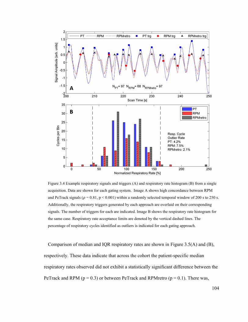
104

Figure 3.4 Example respiratory signals and triggers (A) and respiratory rate histogram (B) from a single

acquisition. Data are shown for each gating system. Image A shows high concordance between RPM

and PeTrack signals (𝜌 = 0.81, p < 0.001) within a randomly selected temporal window of 200 s to 250 s.

Additionally, the respiratory triggers generated by each approach are overlaid on their corresponding

signals. The number of triggers for each are indicated. Image B shows the respiratory rate histogram for

the same case. Respiratory rate acceptance limits are denoted by the vertical dashed lines. The

percentage of respiratory cycles identified as outliers is indicated for each gating approach.

Comparison of median and IQR respiratory rates are shown in Figure 3.5(A) and (B),

respectively. These data indicate that across the cohort the patient-specific median

respiratory rates observed did not exhibit a statistically significant difference between the

PeTrack and RPM (p = 0.3) or between PeTrack and RPMretro (p = 0.1). There was,

105

however, a statistically significant difference between the median respiratory rates

measured with RPM and RPMretro (p = 0.003), as is shown in Figure 3.5(A).

Figure 3.5 Median respiratory rates (A) and IQR (B) for each gating system for the entire cohort. Mean,

±1 SD, and individual measurements are represented as solid-red lines, dashed-gray lines, and gray

points, respectively. P-values produced from paired t-tests are shown in instances where statistically

significant differences were observed.

The IQRs of the respiratory rate distributions, shown in Figure 3.5(B), showed a

significant difference of the respiratory rate IQRs observed with PeTrack compared to

those observed with the RPM and RPMretro. This indicated greater variability in the

observed respiratory rates on a per-patient basis across the cohort. The mean paired

differences were 1.4 breaths/min (p = 0.002) and 1.0 breaths/min (p = 0.04) between

PeTrack and RPM and PeTrack and RPMretro, respectively. No significant differences

were observed for IQR between RPM and RPMretro, suggesting similar patient-specific

variability across the cohort.

The percentage of respiratory cycle outliers for each gating system are shown in Figure

3.6. These data indicate that there was a statistically significant difference between the

RPMretro system with both of the other approaches. These differences gave rise to a

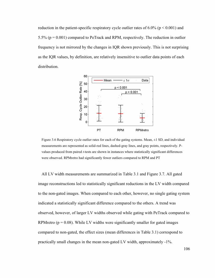
106

reduction in the patient-specific respiratory cycle outlier rates of 6.0% (p < 0.001) and

5.5% (p = 0.001) compared to PeTrack and RPM, respectively. The reduction in outlier

frequency is not mirrored by the changes in IQR shown previously. This is not surprising

as the IQR values, by definition, are relatively insensitive to outlier data points of each

distribution.

Figure 3.6 Respiratory cycle outlier rates for each of the gating systems. Mean, ±1 SD, and individual

measurements are represented as solid-red lines, dashed-gray lines, and gray points, respectively. P-

values produced from paired t-tests are shown in instances where statistically significant differences

were observed. RPMretro had significantly fewer outliers compared to RPM and PT

All LV width measurements are summarized in Table 3.1 and Figure 3.7. All gated

image reconstructions led to statistically significant reductions in the LV width compared

to the non-gated images. When compared to each other, however, no single gating system

indicated a statistically significant difference compared to the others. A trend was

observed, however, of larger LV widths observed while gating with PeTrack compared to

RPMretro (p = 0.08). While LV widths were significantly smaller for gated images

compared to non-gated, the effect sizes (mean differences in Table 3.1) correspond to

practically small changes in the mean non-gated LV width, approximately -1%.

107

Table 3.1 Mean anterior and inferior LV wall widths for each reconstruction method for the entire cohort

as well as for the subset of cases with SI motion ≥ 7 mm. Additionally, the mean differences are shown

for each paired comparison. Comparisons with statistically significant differences (p < 0.05) are written

in bold font.

Images

Mean LV Widths (± SD) [mm]

Cohort SI Motion ≥ 7 mm

Non-Gated 12.3 (2.8) 12.5 (2.3)

PeTrack 12.0 (2.5) 12.0 (2.4)

RPM 11.8 (2.7) 12 (3)

RPMretro 11.8 (2.6) 11.3 (2.3)

Image Pairs

Mean Differences in LV Width (± SD) [mm]

Cohort P SI Motion ≥ 7 mm P

‘PeTrack – Non-Gated’ -0.13 (1.3) 0.02 -0.19 (0.12) > 0.05

‘RPM – Non-Gated’ -0.2 (1.1) < 0.001 -0.22 (0.14) > 0.05

‘RPMretro – Non-Gated’ -0.2 (1.1) < 0.001 -0.48 (0.11) < 0.001

‘PeTrack – RPM’ 0.1 (1.1) > 0.05 0.03 (0.13) > 0.05

‘PeTrack – RPMretro’ 0.1 (1.1) > 0.05 0.29 (0.10) 0.009

‘RPMretro – RPM’ 0.0 (1.1) > 0.05 -0.26 (0.15) 0.08

The comparisons were repeated for the subset of acquisitions where the mean SI LV

motion was ≥ 7 mm (averaged across all gating systems) where the effect sizes were

expected to be larger. These data are provided in the right column of Table 3.1 and shown

graphically in Figure 3.7(B). Within this subset the reduction in LV widths due to gating

was larger compared to that seen in the entire cohort. Compared to the non-gated

measurements, thickness reductions compared to non-gated images ranged from -1.6%

with PeTrack to -3.9% for RPMretro. Within this subset, the differences between

PeTrack and RPM were not statistically significant when compared to the non-gated

images in spite of the increased effect size. This is likely due to the reduced statistical

power of this small subset size. While no differences were observed between PeTrack

and RPM, there was a statistically significant difference between PeTrack and RPMretro

(p = 0.009) as well as a trend toward smaller LV widths with RPMretro compared to

RPM (p = 0.08).

108

Figure 3.7 LV width measurements for both anterior and inferior regions for entire cohort (A) as well as

the subset of cases with mean SI LV motion ≥ 7 mm (B). The means, ± 1 SD ranges, and individual

measurements for each are indicated by the solid-red lines, dashed-gray lines, and gray points,

respectively. Statistically significant p-values, computed from paired t-tests, are indicated.

Table 3.2 SI motion measurements for each gated reconstruction method for the cohort as well as for the

subset of cases with motion ≥ 7 mm. Additionally, the mean differences in SI motion among all paired

comparisons are shown. Statistically significant differences (p < 0.05) are emphasized with bold font.

Images

Mean SI Motion (± SD) [mm]

Cohort SI Motion ≥ 7 mm

PeTrack 4.4 (2.4) 7.6 (2.6)

RPM 4.7 (2.5) 8.3 (2.5)

RPMretro 5.7 (2.6) 9.5 (2.7)

Image Pairs

Mean Differences in SI Motion (± SD) [mm]

Cohort P SI Motion ≥ 7 mm P

‘PeTrack – RPM’ -0.4 (0.3) > 0.05 -0.7 (1.4) > 0.05

‘PeTrack – RPMretro’ -1.4 (1.8) < 0.0001 -1.9 (0.5) 0.008

‘RPMretro – RPM’ 1.0 (2.1) 0.002 1.2 (1.2) > 0.05

The results of the SI motion measurements are provided in Table 3.2 and shown in

Figure 3.8. Across the cohort (left column of Table 3.2 and Figure 3.8(A)) statistically

significant differences were observed between PeTrack and RPMretro (p < 0.0001) as

well as RPMretro and RPM (p = 0.002). The results for the subset of the study with mean

SI LV motion ≥ 7 mm are shown in Figure 3.8(B) and the right column of Table 3.2. For

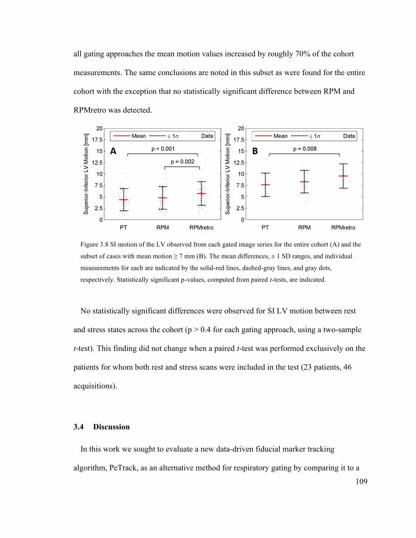
109

all gating approaches the mean motion values increased by roughly 70% of the cohort

measurements. The same conclusions are noted in this subset as were found for the entire

cohort with the exception that no statistically significant difference between RPM and

RPMretro was detected.

Figure 3.8 SI motion of the LV observed from each gated image series for the entire cohort (A) and the

subset of cases with mean motion ≥ 7 mm (B). The mean differences, ± 1 SD ranges, and individual

measurements for each are indicated by the solid-red lines, dashed-gray lines, and gray dots,

respectively. Statistically significant p-values, computed from paired t-tests, are indicated.

No statistically significant differences were observed for SI LV motion between rest

and stress states across the cohort (p > 0.4 for each gating approach, using a two-sample

t-test). This finding did not change when a paired t-test was performed exclusively on the

patients for whom both rest and stress scans were included in the test (23 patients, 46

acquisitions).

3.4 Discussion

In this work we sought to evaluate a new data-driven fiducial marker tracking

algorithm, PeTrack, as an alternative method for respiratory gating by comparing it to a

110

well-accepted hardware-based alternative, RPM. No attempt was made to compare the

respiratory tracking performance to other data-driven approaches, especially those that

use no external markers, as no studies currently exist that reported their performance for

82Rb cardiac MPI studies. Additionally, these approaches are currently not as well

established or widely used as the commercial hardware-based systems. The evaluation of

other data-driven approaches for this application may be explored in future work.

3.4.1 Respiratory Signal and Trigger Measurements

PeTrack respiratory motion signals were significantly correlated with those of the RPM

in nearly all cases (45/50, mean ρ = 0.49). Noticeable discrepancies were noted in some

acquisitions. Discrepancies in the respiratory signals may be attributed to several factors.

Firstly, the temporal resolution is reduced for PeTrack compared to the RPM (2 Hz

compared to 30 Hz) which may have a modest blurring effect on the PeTrack signal.

Secondly, the PeTrack respiratory signal accounts for motion in the inferior-superior and

anterior-posterior directions, which may not always correlate well with the anterior-

posterior motion tracked by RPM. Lastly, the tracking precision with PeTrack is affected,

to some extent, by the radiotracer activity in the patient which leads to substantial

background to the marker’s signal. It follows that there may be some time (tracer

activity) dependence for the tracking precision. A more detailed discussion of the

PeTrack system is included later in this section. The 95% central range of respiratory

rates observed with RPM and PeTrack across the cohort corresponded to 0.07 to 0.5 Hz.

It follows that a 2 Hz sampling rate, which is greater than the Nyquist frequency (1 Hz),

was not expected to lead to aliasing.

111

Some context for the signal correlations reported here can be gleaned from previous

studies involving data-driven respiratory tracking systems that were compared to

hardware-based approaches. Schleyer et al.,140 examined the data-driven spectral analysis

method (SAM) and a modified version referred to as the kinetic respiratory gating

(KRG) method for deriving respiratory signals in 13N-ammonia MPI studies. The latter

was designed specifically to attempt to overcome the typical loss of signal quality in the

early time frames of PET procedures when the tracer distributions are changing rapidly.

They reported mean correlation coefficients of 0.5 ± 0.2 and 0.75 ± 0.08 between the

SAM and KRG versus the RPM system. The SAM results are similar to the mean

correlation coefficient reported in this study. While the KRG method has not yet been

applied to 82Rb MPI studies, its reported success in the early-frames of 13N-ammonia

studies is encouraging. Additionally, the good overall correlation reported in this work

between a data-driven and hardware-based methods has been previously reported in a

study comparing several data-driven respiratory gating methods with a pressure-belt

apparatus in a clinical FDG-PET study for lung lesion detection.112 Mean correlation

coefficients were also reported by Büther et al.,116 in cardiac 18F-FDG studies for the

sensitivity115 and center-of-mass111 data-driven methods with respect to video-camera

monitoring. The authors reported Spearman rank correlation coefficients of 0.65 and 0.68

for the sensitivity and center-of-mass methods, respectively. While these values appear

larger than that reported in this work the author asserted that cardiac PET studies

involving shorter-lived tracers, e.g. 13N-ammonia or H215O, would be expected to reduce

the overall signal quality.

112

Three metrics were used to compare the quality of the respiratory triggers derived using

different gating systems: the median respiratory rates, their corresponding IQRs and the

respiratory cycle outlier rate using our quality control method. Median respiratory rates

are not an indication of performance, but their comparison between the gating methods

can give a sense of the similarity of the output of each. From our results it was found that

generating respiratory triggers retrospectively from the RPM signals led to a small but

statistically significant change in the median respiratory rates. This finding indicates that

the information produced by the RPM was sensitive to the way in which the triggers were

identified/recorded. That said, the mean respiratory rates and the corresponding relative

standard deviations observed with RPM and PeTrack in this study are in good agreement

with those reported for retrospective gating by Didierlaurent et al., while using the RPM

system.161 Based both on trigger-based and image-based metrics we observed overall

improvement in RPM performance following retrospective processing as was reported by

Didierlaurent et al.161 A statistically significant difference was observed for the IQRs of

the respiratory rates distributions suggesting greater variability in the triggers reported

with PeTrack compared to the RPM and RPMretro. The effect size amounted to an

increase in respiratory variability of approximately 1-1.4 breaths/min compared to a

typical respiratory rate of 15 breaths/min. Note that this effect was not found to be

correlated with the reduced motion resolution of PeTrack compared to RPMretro in the

subset of cases with motion ≥ 7 mm.

113

3.4.2 Quality Control

The method used to identify outlier respiratory cycles was inspired by those described

by Boning and Hacker162 for quality control of ECG-gated PET studies. In their

investigation, limits on cycle outliers were estimated based on the cycle rate relative to

individuals’ median respiratory rates. Additional modifications were implemented to

account for the non-Gaussian and irregular nature of the human respiratory patterns,

namely the application of a log-transformation to the data. Interestingly, no literature on

the topic of quality control or cycle rejection of respiratory triggers was found at the time

of the present study. Boning and Hacker have also recommended visual quality control

methods with which physiological explanations of poor ECG-trigger quality can be

inferred, one of which involves inspection of raw signals superimposed with the trigger

events, an example of which was shown in Figure 3.4(A). This process was implemented

for PeTrack and RPM signals for a subset of the acquisitions in this study to identify

trends and/or explanations for cases where respiratory cycle outlier rates were relatively

high between the two gating methods.

A qualitative investigation of the 17 acquisitions where the respiratory cycle outlier

rates observed using RPM or PeTrack differed by more than 10% was performed. Within

this group, 8 cases (47%) indicated that the RPM outlier rate was greater than PeTrack.

Visual inspection of the respiratory signals along with markers of the trigger events,

indicated that some RPM triggers were absent from the list-mode data files. In all but one

of these cases the respiratory signals were smooth and well resolved so while the

explanation of the inability of RPM to trigger at the correct phase is not completely

understood it appears to not be associated with the precision of the optical tracking

114

system. The most extreme example of this issue was identified by an interval of 200

seconds between respiratory triggers. A less extreme example of this was observed for

the example case described in Figure 3.4. By visual comparison, it is evident that

respiratory triggers are missing from the RPM trace and those that are present occur at

inconsistent phases of the respiratory cycle. In stark contrast to the RPMretro data that

are shown, respiratory cycles occurring at 210 s, 217 s, 225-232 s and 235 s are not

marked by respiratory triggers. In this example, LV motion was severely underestimated

while gating with RPM compared to PeTrack and then recovered after retrospective

processing to generate the respiratory triggers. This can be seen in Figure 3.9 which

shows a common coronal slice for each of the non-gated, PeTrack, RPM, and RPMretro

images as well as a plot of IS LV displacement at each respiratory gate. Increased

blurring at the anterior LV region as well as increased uptake non-uniformity at the

inferior LV region are clearly visible in the non-gated and RPM images compared to that

observed with PeTrack or RPMretro. The number of cases for which the respiratory cycle

outlier rate was >10% for RPM compared to PeTrack was reduced from 8 to 1 after

deriving respiratory trigger retrospectively.

Two acquisitions from the initial cohort were excluded from this study as they had

either no, or too few, RPM triggers to synchronize the respiratory signal data to the list-

mode data. Technical limitations associated with this device have been previously

reported101,163 where signal quality was reduced or signals were not recorded due to

baseline drifts in the patient position, operator errors, restrictions associated with patient

size, involuntary patient motion, and the use of warming blankets. In the 9 cases (53%)

where the cycle outlier rate was greater for PeTrack than for the RPM, the cause was

115

typically attributed to reduced signal-to-noise ratio in the motion trace of the fiducial

marker throughout the acquisition.

Figure 3.9 Inter-gate motion comparison for the exemplary case selected for Figure 3.4. On the left,

coronal views at end-expiration are shown for comparison from non-gated, PeTrack, RPM, and

RPMretro images. Note that the non-gated images were statistically sampled such that they were noise-

matched with the gated images. On the right, the superior-inferior displacement of the LV as observed

across the six gates using each gating system is plotted: PeTrack in blue squares, RPM in red circles, and

RPMretro in gray triangles. Displacements were recorded with respect to the corresponding phase-

averaged position. In this example the motion extent observed while gating with PeTrack and RPMretro

was substantially larger than that observed with RPM. Note that the images shown here were smoothed

with a 10 mm FWHM 3D Gaussian kernel for display purposes.

The respiratory cycle outlier rates of both systems exceeded 10% in 7/50 cases (14%)

and these cases exhibited recurring instances of irregularities in the respiratory signals.

These irregularities manifested as extended breath-holds, usually at inspiration, or steep

gradients in the signals that may be associated with abrupt whole-body patient motion or

coughing.

Statistically significant negative correlations were found between the paired respiratory

cycle outlier rates and the paired LV motion measurements across the entire cohort

116

between PeTrack and RPM (𝜌 = -0.45, p = 0.001) as well as PeTrack and RPMretro (𝜌 =

-0.49, p < 0.001), indicating that increases in the outlier rates led to reductions in the

detected LV motion between the systems, and vice versa. This intuitive finding supports

the validity of the respiratory cycle outlier rate as a metric of respiratory tracking quality.

Outlier respiratory cycles were not excluded from the reconstructions in this study but the

effect of such an action remains as an interesting research question and warrants further

investigation.

3.4.3 Image based motion estimates

From the reconstructed images there appeared to be no statistically significant

difference in LV thickness measurements, indicating no systematic difference in blurring

between PeTrack and RPM gated images. This was not the case, however, when

considering only those acquisitions with more severe respiratory motion, i.e. ≥ 7 mm. For

this subset, no differences in LV widths were detected between either PeTrack or RPM

and non-gated images but differences, i.e. smaller widths, were detected for RPMretro.

This finding was supported by the reduced motion resolution of PeTrack in this subset.

The mean SI LV displacements observed in this study were in excellent agreement with

value of 4.6 mm reported by Wells et al., for a comparatively larger cohort of 82Rb and

13N-ammonia MPI studies.101 Additionally, no statistically significant difference was

detected in the extent of motion between rest and stress states for 82Rb scans, as was the

case in this study. Larger mean LV displacements were reported by Büther et al., in a

cohort of 17 patients while using the sensitivity and center-of-mass based gating

methods, but the radiotracer used was 18F-FDG which has improved spatial resolution

117

over 82Rb making comparisons difficult. This apparent increase in SI LV displacement is

likely associated, however, with increased number of respiratory gates (10 gates rather

than 6) which would enhance the motion resolution for the gated images.158

3.4.4 Considerations for PeTrack

Most data-driven gating algorithms derive motion signals directly from the activity of

the tracer within the patient and while this approach may explicitly estimate motion of the

organs of interest, the accuracy/precision of the signal is highly dependent on the tracer

distribution which varies in time.140 The use of an external marker with a long-lived

positron emitting isotope has been proposed for use as a motion tracking tool in a

previous study.122 While differences in phase and/or amplitude in the motion of an

external marker compared to that of the thoracic organs or lesions have been

reported102,105,164, the external motion measured at the abdomen has been shown to have

good correlation with inferior-superior motion of internal regions of interest.102,122,164

There are several factors that can limit the effectiveness of the PeTrack system for

patient-motion tracking. As was mentioned previously, since PeTrack relies on the

positron-emission signal of a fiducial marker there exists substantial interference in the

form of LORs from the radiopharmaceutical tracer. Selecting for coincidence events

associated with the marker alone is not a trivial task. Cardiac perfusion studies at our

institution that make use of 82Rb can produce scanner count rates in excess of 107 counts

per second, at which time the activity of the fiducial marker used in this study

corresponds to less than 0.01% of the scanner count rate. Although the current

implementation of PeTrack includes a background rejection step that excludes most of

118

the LORs originating in the patient, the tracer background in some studies may reduce the

signal-to-noise ratio of the marker too much to allow PeTrack to track the marker with

sufficient precision. This effect can be accounted for by the exclusion of the initial

portion of the acquisition that includes the peak count rate from the image reconstructions

(as was essentially the case in this study). In the case of 82Rb, which has a half-life of 76

s, the exclusion of the first 90 - 120 s of the acquisition required for clearance of the LV

blood pool is generally sufficient for this purpose.165 Additionally, when using

radiotracers with short half-lives the position of the marker can be tracked in reverse, i.e.

from end of the acquisition to the beginning, to begin when the SNR of the marker’s

signal is much more favorable. This challenge is expected to be less significant for

longer-lived tracers that exhibit a much narrower dynamic range of count rates

throughout the acquisition. The conditions in this work, therefore likely evaluated

PeTrack performance under one of the most challenging settings. Regardless, this and

other work157,166 have demonstrated feasibility in clinical practice, especially for the post-

bolus stages of a cardiac acquisition. Büther and colleagues122 did not report similar

difficulties while tracking radioactive fiducial markers in projection space although they

reported using markers with activity that was roughly three times greater than those in

this study. Additionally, they placed the markers on structural supports to separate the

markers from the skin of the patients which resulted in a greater patient setup complexity,

and potential interference with scatter correction.

Another important consideration is the placement of the PeTrack marker on a patient.

As the geometric sensitivity of the scanner decreases at the edge of the axial field of

view, it follows that placement of the marker too near to the edge (i.e. too inferior or

119

superior) will lead to a significant signal reduction. Placement of the marker too near to

the heart in perfusion studies may also lead to complication as the activity of the tracer

accumulates in the myocardium leading to a higher interference level for the PeTrack

system throughout the scan. To help compensate for these issues one could simply

increase the activity of the fiducial marker to increase the ratio of its signal over that of

the administered PET tracer. At the Cardiac PET Centre at UOHI, the use of low activity

external markers is part of the clinical imaging protocol as a quality control measure. As

these data were collected as part of a clinical quality improvement study, the use of

higher activity markers was not considered. Apart from increasing the marker activity to

enhance tracking precision, the marker should ideally be placed in the middle of the axial

field of view but distally from regions where high uptake is expected, e.g. the heart in

perfusion studies. Training of technologists is essential to ensure optimal marker

placement on the patient. Cardiac PET studies with tracers that are administered with

lower initial activities may be ideal candidates for motion tracking with PeTrack.

Additionally, the use of long bore PET systems will enable better separation between

heart and marker placement while ensuring both remain well within the field of view. A

previously reported technical limitation of the RPM is the reduced visibility of the

reflective marker in long-bore scanners which may preclude its use on these systems.79

3.4.5 Clinical Use of PeTrack for Respiratory Gating

While this work focused on evaluating PeTrack as an alternative to hardware-based

respiratory gating devices, another practical application, as demonstrated in our practice,

is to use both systems in concert. This approach affords the option to select the more

120

reliable of the two gating sources on a post-hoc basis and/or use the respiratory signal

from PeTrack to supplement the respiratory triggers produced by the RPM system. It was

noted previously that the RPM and PeTrack systems were configured to trigger at

different respiratory phase which may complicate the combination of the respiratory

tracking data of the two. As was shown, this challenge could be overcome by

retrospectively processing the RPM signals to generate respiratory triggers at end-

expiration using the same utilities that have been used for PeTrack. The use of an external

marker for PeTrack increases the complexity of patient setup compared to alternative

data-driven approaches but the added difficulty is minimal as no support structure or

adhesives are needed. Unlike many data-driven methods that have been proposed, the

PeTrack signal can additionally be used to track whole-body motion of the patient as the

absolute 3D position of the marker is determined as opposed to temporal fluctuations of

signal intensity in list-mode or projection spaces. Some early work on this application has

been performed already167 and will be further explored in future investigations. In our

clinic fiducial markers are already used in all cardiac PET scans as an indication of

patient motion, particularly for dynamic acquisitions. It follows that PeTrack can be

applied without modification to current patient setup procedures. Beyond placing the

marker on the patient, technologists must verify that the marker is within the axial field-

of-view. This task is satisfied by visual inspection of the initial scout CT scan which is

used in the clinical workflow for patient positioning prior to each PET acquisition. When

compared to the RPM system, significantly less setup is required as PeTrack requires no

setup of dedicated hardware or staff monitoring during imaging.

121

3.5 Conclusion

A data-driven respiratory gating system was developed that utilizes a low activity,

positron emitting, fiducial marker and we compared its performance to an established

hardware-based system in a practical clinical setting. Despite the challenging conditions

posed by 82Rb cardiac PET/CT for data-driven approaches, PeTrack appears feasible for

retrospective respiratory gating with no practical loss in the ability to capture patient

respiratory motion or in respiratory-gated image quality compared to the established real-

time gating available with the RPM system. The performance of both PeTrack and

prospective RPM was generally reduced in comparison to the retrospective RPM

approach. This data-driven approach has the potential to reduce the need for expensive

ancillary hardware systems to monitor respiratory motion but could benefit from

additional implementation development.

122

Chapter 4 Whole-Body Motion Correction in Myocardial Perfusion

Imaging with PET/CT

In this and the following chapter, the ability of PeTrack to detect and estimate whole-

body motion was considered. The content of this chapter is largely based on work that

was presented at the IEEE Nuclear Science Symposium and Medical Imaging Conference

in 2018167 and 2019168. Conference record publications were submitted following each of

these events. Some figures from these conference record publications are reproduced here

with permission from the authors.

4.1 Motivation

Various studies have been reported that sought to measure the prevalence and effects of

patient motion in cardiac PET/CT, the results of which indicated that motion was present

in as high as 52% of patients studied.82 Others indicated that motion prevalence and

severity was affected by the state of rest or stress in the patient, and in the stress cases by

choice of exercise or pharmacologic stressing agents used.148,149,169 Average whole-body

motion magnitudes have also been reported in the range of 6 to 10 mm82,148 but with

maximum magnitudes at or greater than 18 mm.82,169

At a minimum, it has been recommended in cardiac PET/CT that motion be assessed

visually while others recommend that motion correction strategies be implemented,

particularly while patients are in a stress state after pharmacological vasodilation or

treadmill exercise testing. Although several motion correction strategies have been

proposed147–149 translation into clinical practice is uncommon.148 Typically, motion

correction is attempted by spatial registration of dynamic images of pre-defined

123

durations.81,147–149 As a result, they are neither able to correct for intra-frame motion nor

do they address the issue of PET-CT misalignment. Indeed, there is a need for a whole-

body motion correction algorithm in PET/CT that can correct for patient motion and

PET-CT mis-alignment prior to image reconstruction.169

We sought to evaluate a WBM correction method with information from tracking

fiducial markers using the data-driven Positron Emission Tracking (PeTrack) algorithm.

Within this current framework 3D translational motion correction is achievable without

the need for a priori choice of multiple acquisition frames. Additionally, image

registration techniques are not required to estimate patient motion. This latter feature is

useful as the spatial registration of PET images with limited count statistics is challenging

due to increased image noise as well as changes in image intensity associated with tracer

dynamics.170 A combination of phantom and patient data was used to demonstrate this

approach. As PeTrack has only been applied previously on studies using 82Rb as the PET

tracer, a secondary objective of this study was to validate the tracking performance of

PeTrack in clinical data sets which used 13N-ammonia as a perfusion tracer.

4.2 Methods

4.2.1 Whole-Body Motion Correction Framework

Unlike what was described in the previous chapter where gated images were

reconstructed to compensate for motion, here the MAF motion correction paradigm was

implemented such that individual reconstructed frames are spatially aligned using motion

information provided by PeTrack.

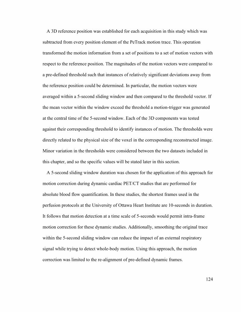
124

A 3D reference position was established for each acquisition in this study which was

subtracted from every position element of the PeTrack motion trace. This operation

transformed the motion information from a set of positions to a set of motion vectors with

respect to the reference position. The magnitudes of the motion vectors were compared to

a pre-defined threshold such that instances of relatively significant deviations away from

the reference position could be determined. In particular, the motion vectors were

averaged within a 5-second sliding window and then compared to the threshold vector. If

the mean vector within the window exceed the threshold a motion-trigger was generated

at the central time of the 5-second window. Each of the 3D components was tested

against their corresponding threshold to identify instances of motion. The thresholds were

directly related to the physical size of the voxel in the corresponding reconstructed image.

Minor variation in the thresholds were considered between the two datasets included in

this chapter, and so the specific values will be stated later in this section.

A 5-second sliding window duration was chosen for the application of this approach for

motion correction during dynamic cardiac PET/CT studies that are performed for

absolute blood flow quantification. In these studies, the shortest frames used in the

perfusion protocols at the University of Ottawa Heart Institute are 10-seconds in duration.

It follows that motion detection at a time scale of 5-seconds would permit intra-frame

motion correction for these dynamic studies. Additionally, smoothing the original trace

within the 5-second sliding window can reduce the impact of an external respiratory

signal while trying to detect whole-body motion. Using this approach, the motion

correction was limited to the re-alignment of pre-defined dynamic frames.

125

Figure 4.1 An example 1D motion trace is shown from the patient cohort to demonstrate the production

of motion triggers after applying the moving mean filter. To simplify the example, only the motion the

left-right direction is shown here. The original and filtered traces are depicted by blue and black curves,

respectively. The motion triggers are shown as vertical, dashed lines. The motion thresholds are also

indicated as the vertical limits of the gray bands which span the domain of the plot.

As was stated previously, this motion correction framework was designed to

compensate for motion-induced CTAC misalignment as well as the loss in signal-to-noise

ratio in the target tissues. To achieve this, a separate image was reconstructed for each

‘motion frame’, i.e. a reconstructed frame that includes the data bound by two motion

triggers, that was identified and were registered and averaged post-reconstruction using

the motion vectors produced by PeTrack averaged over the duration of each motion

frame. In the event that non-adjacent motion frames were found to correspond to the

same position, a form of whole-body motion amplitude gating was applied. In this

approach, the raw list-mode data were combined to reduce to the total number of

reconstructed frames. If this occurred, corrections for radioactive decay, dead time, and

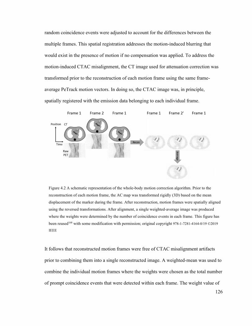
126

random coincidence events were adjusted to account for the differences between the

multiple frames. This spatial registration addresses the motion-induced blurring that

would exist in the presence of motion if no compensation was applied. To address the

motion-induced CTAC misalignment, the CT image used for attenuation correction was

transformed prior to the reconstruction of each motion frame using the same frame-

average PeTrack motion vectors. In doing so, the CTAC image was, in principle,

spatially registered with the emission data belonging to each individual frame.

Figure 4.2 A schematic representation of the whole-body motion correction algorithm. Prior to the

reconstruction of each motion frame, the AC map was transformed rigidly (3D) based on the mean

displacement of the marker during the frame. After reconstruction, motion frames were spatially aligned

using the reversed transformations. After alignment, a single weighted-average image was produced

where the weights were determined by the number of coincidence events in each frame. This figure has

been reused168 with some modification with permission; original copyright 978-1-7281-4164-0/19 ©2019

IEEE

It follows that reconstructed motion frames were free of CTAC misalignment artifacts

prior to combining them into a single reconstructed image. A weighted-mean was used to

combine the individual motion frames where the weights were chosen as the total number

of prompt coincidence events that were detected within each frame. The weight value of

127

each bin of data to the final image was the number of coincidence counts. A schematic

diagram of this workflow is presented in Figure 4.2. In this diagram only three frames

were considered, the second of which is shown as being shifted away from the others.

4.2.2 Validation Using an Anthropomorphic Torso Phantom

Myocardial perfusion studies were simulated with the use of an anthropomorphic torso

phantom that included a cardiac insert that models the left-ventricle of the heart.

Acquisitions were carried out on a GE Discovery 690 PET/CT scanner (Waukesha, WI)

with time-of-flight PET and list-mode capability after the injection of 3 MBq and 27

MBq of 18F-FDG into the cardiac insert and thorax cavities, respectively. Whole-body

motion was simulated by physically translating the phantom during the acquisition.

Motion was applied in the three cases along superior-inferior and lateral directions as

well as diagonally along both. One motion-free acquisition was used as a reference for

comparison for the acquisitions with motion both before and after motion correction.

Translations were approximately 5 mm in magnitude and occurred at 60 second intervals.

Images were reconstructed using the vendor’s standard 3D OSEM offline reconstruction

toolbox with a transaxial and axial field-of-view of 500 mm and 150 mm, respectively,

and a 128 x 128 x 47 matrix size. Post-reconstruction filtering was applied using a 5 mm

FWHM Gaussian smoothing kernel and nearest neighbour weighted averaging in the

axial direction (the relative nearest neighbour weights were 1, 2, 1).

Motion tracking was performed at a frequency of 2 Hz using the PeTrack algorithm to

calculate the position of a radioactive fiducial marker (22Na, ~30 kBq) placed on the

anterior surface of the phantom. A reference position was recorded at the beginning of

128

the acquisition where emission data were aligned with CT data used for attenuation

correction. The motion thresholds that were used were 3.91 mm and 3.27 mm in the

lateral direction and axial directions, respectively. These thresholds correspond to the

physical sizes of the voxels in each of the directions of motion that was considered.

Motion detection and estimation were performed using the approach described above.

4.2.3 Application to 13N-Ammonia Perfusion Studies

The rest and dipyridamole-stress scans of three patients (N = 3) were used in this study

(weight 135-158 kg, height 173-178 cm). Two patients were imaged on a GE Discovery

690 PET/CT system and one on a GE Discovery 600 PET/CT system. Patients were

injected with 3 MBq/kg of 13N-ammonia for each of the rest and stress imaging protocols.

The acquisition duration for both protocols was 20 min commencing with tracer

administration. A CT image acquired prior to the rest PET acquisitions was used for

attenuation correction for both rest and stress images. Note that the patients are labelled

as A, B, and C throughout this chapter.

Image reconstructions were performed offline using the vendor’s reconstruction

toolbox. A 3D OSEM algorithm with 16 sub-iterations and 4 iterations was used. The

dimensions of the images were 128 × 128 × 47 voxels with sizes of 3.91 × 3.91 × 3.27

mm3, respectively. Corrections for attenuation, random and scatter prompt coincidences

were applied. Post-reconstruction smoothing was not applied to the images; an exception

to this is mentioned below. Reconstructions ignored the early time phase where the tracer

has not yet been taken up in the tissue. These start times were 120 s and 300 s for the

Discovery 690 and Discovery 600 scanners, respectively.

129

In this study, the same fiducial marker (22Na, ~30 kBq) was placed on the chest, to the

right of midline, on each patient. The motion thresholds were reduced for the clinical data

sets as compared to those of the phantom experiment. The motion simulated in the

phantom studies represented a relatively extreme case and the transitions were rapid. As

motion is often not so well defined for humans, the thresholds for detecting motion were

relaxed. The thresholds were set to half the voxel sizes, 1.96 mm and 1.64 mm for

transaxial and axial directions, respectively, for the clinical data sets.

A reference position was determined as the mean position of the marker during the

entire reconstructed frame (120 s – 1200 s and 300 s to 1200 s for acquisitions on the GE

Discovery 690 and 600 scanners, respectively). This was done so that the PET reference

position has the best alignment with the CT image used for attenuation correction. This

assumption is based on the use of a 3D displacement vector stored in the metadata of the

raw files used in the offline reconstruction. This 3D vector was produced by technologists

in the clinic to rigidly register the CT image to the PET image to enhance the quality of

the attenuation correction.

4.2.4 Quantitative Measurements

Several image-based quantitative measurements were performed to evaluate the quality

of the image reconstructions both prior to and following motion correction. The

following measurements were performed for both the phantom and patient data sets.

Several additional measurements, which will be described below, were exclusively

performed on the patient images. All measurements were performed after reorienting the

image volume into the short-axis representation. All motion-corrected images were

130

reoriented using the transformation matrix that was used for the corresponding non-

corrected image to enhance spatial agreement between the pair; this was done especially

for comparison of LV thicknesses within specific segments. The reorientation method

was described previously in Section 3.2.4. LV wall-thicknesses and contrast-to-noise

ratios (CNR) were measured as quality metrics of the images.

The LV wall thicknesses were measured using a modified version of the approach

described in Section 3.2.7. Unlike the method used in Chapter 3, radial profiles emanated

from the center of the LV blood pool and extended beyond the epicardium. Profiles were

produced at 16 equally spaced angular positions on 14 short axis slices. Note that 20

angular samples were acquired for some clinical images where patients had left ventricles

that were considerably larger than the of the anthropomorphic phantom. The rationale for

not applying post-reconstruction smoothing was to not affect these thickness

measurements in the reconstructed images. An example of the profiles is provided in

Figure 4.3. While a multi-resolution approach was once again used, there was no

averaging among adjacent profiles as was described in Section 3.2.7. Individual

measurements were averaged based on the left-ventricular segment to which they

belonged, i.e. there are multiple radial profiles belonging to each segment. The American

Heart Association 17-segment model47 was used. The apex was excluded from phantom

measurements due to the presence of an air bubble within the model LV wall of the

phantom that was completely vacant of activity. Additionally, as the curvature of the

apex did not lend itself to the radial sampling method, it was also not performed among

the clinical data set.

131

Figure 4.3 Diagram of the radial profile locations cast on the reoriented image volumes for the purpose

of making LV thickness measurements. Image A shows a single short-axis slice on which four radial

profiles can be seen originating at the LV center and spanning outward across the LV wall. Image B

shows a horizontal long-axis image slice depicting the series of short axis slices that were used. The

figure is derived from the reference trial reconstruction of the anthropomorphic phantom. A region

within the model LV wall can be seen within the apex to be void of activity; this region corresponds to

an air-bubble. Note that these profile indicators are only qualitative representations of the profile

locations that were actually used for the measurements.

Contrast-to-noise ratios were calculated as the difference in the mean activity

concentrations between the LV and a background volume of interest (𝐴𝐵𝐾𝐺𝐷 ) divided by

the standard deviation measured in the background (𝜎𝐴,𝐵𝐾𝐺𝐷).

𝐶𝑁𝑅 =

𝐴𝐿𝑉 − 𝐴𝐵𝐾𝐺𝐷

𝜎𝐴,𝐵𝐾𝐺𝐷

Eq. 0.1

The LV was segmented using the radial profile fitting procedure that was used to

measure the LV thicknesses. From each radial profile, the coordinates corresponding to

the extent of one FWHM about the centroid were recorded. The inner and outer limits

from each profile were used to construct two polygonal masks on each short-axis slice

that was sampled. The two masks roughly correspond to the endocardial and epicardial

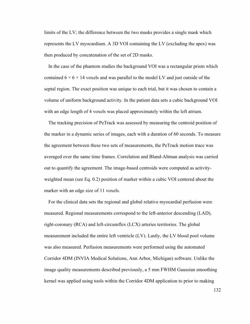
132

limits of the LV; the difference between the two masks provides a single mask which

represents the LV myocardium. A 3D VOI containing the LV (excluding the apex) was

then produced by concatenation of the set of 2D masks.

In the case of the phantom studies the background VOI was a rectangular prism which

contained 6 × 6 × 14 voxels and was parallel to the model LV and just outside of the

septal region. The exact position was unique to each trial, but it was chosen to contain a

volume of uniform background activity. In the patient data sets a cubic background VOI

with an edge length of 4 voxels was placed approximately within the left atrium.

The tracking precision of PeTrack was assessed by measuring the centroid position of

the marker in a dynamic series of images, each with a duration of 60 seconds. To measure

the agreement between these two sets of measurements, the PeTrack motion trace was

averaged over the same time frames. Correlation and Bland-Altman analysis was carried

out to quantify the agreement. The image-based centroids were computed as activity-

weighted mean (see Eq. 0.2) position of marker within a cubic VOI centered about the

marker with an edge size of 11 voxels.

For the clinical data sets the regional and global relative myocardial perfusion were

measured. Regional measurements correspond to the left-anterior descending (LAD),

right-coronary (RCA) and left-circumflex (LCX) arteries territories. The global

measurement included the entire left ventricle (LV). Lastly, the LV blood pool volume

was also measured. Perfusion measurements were performed using the automated

Corridor 4DM (INVIA Medical Solutions, Ann Arbor, Michigan) software. Unlike the

image quality measurements described previously, a 5 mm FWHM Gaussian smoothing

kernel was applied using tools within the Corridor 4DM application to prior to making

133

these measurements. No manual interventions regarding LV segmentation or

reorientation were performed while using Corridor 4DM. The LV blood pool volumes

were calculated as the volume of the inner, or endocardial, mask that was described

previously.

4.3 Results

4.3.1 Motion Tracking Validation

The axial and lateral components of the PeTrack motion traces for the four phantom

acquisitions are shown in Figure 4.4. Changes in the anterior-posterior position were not

included in the experiment so this component of the trace is not shown. The axial

components shown in Figure 4.4(A) provide clear demonstration of the instances of

motion (and non-motion in the Reference and Lateral cases). The lateral motion

component did not demonstrate the same level of tracking precision in the diagonal

motion case. The correlation and Bland-Altman analyses, shown in

Figure 4.5, indicated excellent agreement between the marker displacements reported

by PeTrack and those measured from dynamic image reconstructions. The correlation

coefficient (ρ) of 0.96 and a RMSE of 1.1 mm was observed between the two sets of

measurements. The Bland-Altman plot shows that there is no statistically significant

difference between the two sets of motion measurement as determined by a two-tailed,

paired, Student’s t-test. Across all three trials the mean bias was -0.26 mm, well below

the size of a single voxel. Only the dominant motion dimension is used for each case, e.g.

134

only axial motion was considered for the Diagonal case.

Figure 4.4 Phantom motion trace derived from PeTrack algorithm. Images A and B depict the axial and

lateral displacements as a function of time during the acquisitions. Traces are shown for each acquisition:

reference (blue); axial motion (red); lateral motion (yellow); and diagonal motion (purple).

Figure 4.5 Correlation (A) and Bland-Altman (B) plots for the phantom study indicating the agreement

of motion measured using PeTrack to that measured in each of the non-corrected (Dynamic) ‘motion-

frames’. Measurements for the axial, lateral, and diagonal motion trials are indicated by red, yellow and

purple points, respectively. Plot A contains a grey line of identity and a black line of best fit. Only the

dominant motion component was used for each case, e.g. axial motion is considered for the Diagonal

case. In plot B, the paired differences between the dynamic image and PeTrack measurements are

denoted by ‘∆’.

135

The quality of the PeTrack motion tracking for 13N-ammonia studies was evaluated in a

similar fashion except that the marker displacements were determined from reconstructed

dynamic series with 1-minute frames. From each, the activity-weighted centroid of the

marker and its standard deviation (as per Eq. 0.1) were determined from within a cubic

volume of interest (VOI) set around the marker. The activity-weighted mean and standard

deviations were defined earlier in Section 3.2.7. The VOI had an edge size of 11 voxels.

An example of these measurements is shown in Figure 4.6 where a high concordance

between the PeTrack and image-based measurements can be observed. These data were

produced for all 6 acquisitions in this study. Bland-Altman (see Figure 4.7) and

correlation analyses indicated a Pearson correlation coefficient of 0.91 (p < 0.0001),

RMSE of 0.77 mm, mean paired difference of 0.02 mm with limits of agreement (±

1.96SD) of [-1.49,1.59] mm; all of which indicate excellent agreement.

136

Figure 4.6 Comparison of marker 3D displacements from PeTrack (PT) and image-based (Img)

measurements for the stress acquisition of patient B. Image measurements were made from dynamic

reconstructions of the entire acquisition with 1-minute frames. Symbols with error bars indicate the

centroid and ±1 SD limits of the marker in each dimension (RL = right-left, AP = anterior-posterior, IS =

inferior-superior) for each of the frames. Note that the standard deviations of the centroids were

calculated by using Eq. 0.1. This figure has been reused168 with permission and was modified from its

original version; original copyright 978-1-7281-4164-0/19 ©2019 IEEE

Figure 4.7 Correlation (A) and Bland-Altman (B) plots comparing PeTrack and image-based marker

displacements for all human acquisitions. The PeTrack displacements shown here were averaged over

the 1 min duration of each dynamic frame. The paired differences in B were computed as ‘PeTrack -

Image’. The Bland-Altman plot shows excellent agreement giving strong evidence for tracking quality

with PeTrack in this cohort.

137

4.3.2 LV Wall Thickness and Blood Pool Volume Comparison

To emphasize the effects of motion among the phantom acquisitions 17-segment polar

maps of the LV were produced wherein the value of each segment corresponds to the

change in thickness compared to that of the reference image. These are shown in Figure

4.8. For each non-corrected case (sub images A, C, and D) the changes in thickness are

clearly shown to predominantly follow the direction of motion, e.g. along the anterior-

inferior (A-I) direction for the axial motion case. The motion-corrected polar maps

indicated a much closer agreement with the reference image measurements, as indicated

graphically by segment colours that are less intense and closer to white.

A summary of the LV thicknesses for the four phantom acquisitions is provided in

Table 4.1. The values represent the means across each of 16 LV segments that were

sampled. The mean values for the reference and motion-corrected images demonstrate

good agreement whereas those of the non-corrected images exhibit substantial increases.

Paired Student’s t-tests were performed between the thickness measurements of each trial

case compared to the reference where LV thickness measurements were paired by

segment. All non-corrected images indicated significant thickness increases compared to

the reference. A significant difference was also detected for the diagonal motion-

corrected image which suggested some residual blur that was not adequately

compensated. That said, the mean paired differences for this case was 0.8 ± 1.2 mm,

which is a small effect compared to the mean LV thickness of the reference case (14.3

mm). The mean paired differences for the non-corrected diagonal motion case was 4 ± 4

mm and represents a much larger effect.

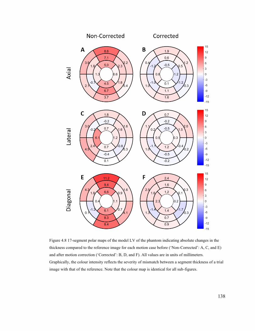
138

Figure 4.8 17-segment polar maps of the model LV of the phantom indicating absolute changes in the

thickness compared to the reference image for each motion case before (‘Non-Corrected’: A, C, and E)

and after motion correction (‘Corrected’: B, D, and F). All values are in units of millimeters.

Graphically, the colour intensity reflects the severity of mismatch between a segment thickness of a trial

image with that of the reference. Note that the colour map is identical for all sub-figures.

139

Table 4.1 LV thicknesses measured for each phantom trial averaged among all 16 segments. Standard

deviations (SD) are also provided. Reported p-values correspond to a two-tailed paired Student’s t-test

for each trial compared to the reference measurements – data were paired by segment for these tests. The

image label ‘MC’ indicates motion correction.

Image LV Thickness

Mean ± SD [mm]

p

Reference 14.3 ± 1.8 -

Axial 17.5 ± 1.4 0.0002

Axial – MC 14.6 ± 1.7 0.4

Lateral 15.8 ± 1.9 0.009

Lateral – MC 14.7 ± 1.7 0.13

Diagonal 18.3 ± 1.6 0.0009

Diagonal – MC 15.1 ± 2.0 0.02

The analogous LV thickness measurements within the clinical dataset are shown in

Table 4.2. The changes were relatively small with a mean, minimum and maximum

paired difference of -0.2 mm, 0.0 mm, and -1.0 mm, respectively. Negative values imply

smaller thicknesses after motion correction. The most substantial changes in thickness

were observed for the stress scans of patients B and C: -0.6 ± 0.5 mm, and -0.7 ± 1.3 mm,

respectively. Statistically, only the stress scan of Patient B corresponded to a significant

difference (p = 0.0002). The measurements of the stress scan of Patient C, however,

indicate a trend toward narrower LV thicknesses after motion correction (p = 0.05).

Several metrics of patient motion were also tabulated for the cohort to provide context for

the thickness measurements. The number of recorded motion-triggers, the number of

motion-frames, and the Euclidean magnitude of the maximal displacements are shown in

Table 4.2.

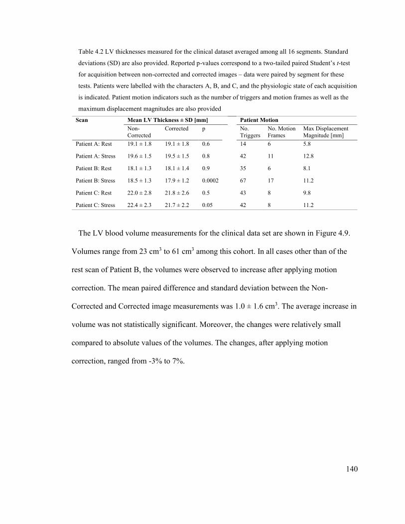
140

Table 4.2 LV thicknesses measured for the clinical dataset averaged among all 16 segments. Standard

deviations (SD) are also provided. Reported p-values correspond to a two-tailed paired Student’s t-test

for acquisition between non-corrected and corrected images – data were paired by segment for these

tests. Patients were labelled with the characters A, B, and C, and the physiologic state of each acquisition

is indicated. Patient motion indicators such as the number of triggers and motion frames as well as the

maximum displacement magnitudes are also provided

Scan Mean LV Thickness ± SD [mm] Patient Motion

Non-

Corrected

Corrected p No.

Triggers

No. Motion

Frames

Max Displacement

Magnitude [mm]

Patient A: Rest 19.1 ± 1.8 19.1 ± 1.8 0.6 14 6 5.8

Patient A: Stress 19.6 ± 1.5 19.5 ± 1.5 0.8 42 11 12.8

Patient B: Rest 18.1 ± 1.3 18.1 ± 1.4 0.9 35 6 8.1

Patient B: Stress 18.5 ± 1.3 17.9 ± 1.2 0.0002 67 17 11.2

Patient C: Rest 22.0 ± 2.8 21.8 ± 2.6 0.5 43 8 9.8

Patient C: Stress 22.4 ± 2.3 21.7 ± 2.2 0.05 42 8 11.2

The LV blood volume measurements for the clinical data set are shown in Figure 4.9.

Volumes range from 23 cm3 to 61 cm3 among this cohort. In all cases other than of the

rest scan of Patient B, the volumes were observed to increase after applying motion

correction. The mean paired difference and standard deviation between the Non-

Corrected and Corrected image measurements was 1.0 ± 1.6 cm3. The average increase in

volume was not statistically significant. Moreover, the changes were relatively small

compared to absolute values of the volumes. The changes, after applying motion

correction, ranged from -3% to 7%.

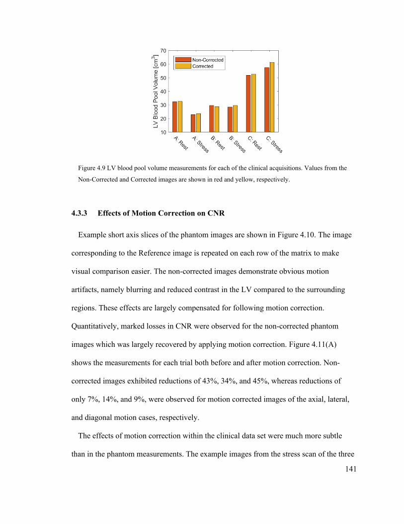
141

Figure 4.9 LV blood pool volume measurements for each of the clinical acquisitions. Values from the

Non-Corrected and Corrected images are shown in red and yellow, respectively.

4.3.3 Effects of Motion Correction on CNR

Example short axis slices of the phantom images are shown in Figure 4.10. The image

corresponding to the Reference image is repeated on each row of the matrix to make

visual comparison easier. The non-corrected images demonstrate obvious motion

artifacts, namely blurring and reduced contrast in the LV compared to the surrounding

regions. These effects are largely compensated for following motion correction.

Quantitatively, marked losses in CNR were observed for the non-corrected phantom

images which was largely recovered by applying motion correction. Figure 4.11(A)

shows the measurements for each trial both before and after motion correction. Non-

corrected images exhibited reductions of 43%, 34%, and 45%, whereas reductions of

only 7%, 14%, and 9%, were observed for motion corrected images of the axial, lateral,

and diagonal motion cases, respectively.

The effects of motion correction within the clinical data set were much more subtle

than in the phantom measurements. The example images from the stress scan of the three

142

patients are shown in Figure 4.12. Motion correction led to an average (percent) increase

in CNR of 11.3%, with a minimum and maximum of -13.9% and 61.2%, respectively.

The CNR measurements for each individual image are shown in Figure 4.11(B).

Figure 4.10 Example short axis images from the four phantom acquisitions. The Reference, Non-

Corrected, and Corrected images for each motion case are shown to emphasize the effects of motion

correction on this data set. All images are displayed on the same intensity range. This figure has been

reused167 with permission; original copyright 978-1-5386-8495-5/18 ©2018 IEEE.

143

Figure 4.11 CNR bar plots for the phantom (A) and 13N-ammonia (B) acquisitions. Reference, non-

corrected and motion-corrected data are shown in blue, orange, and yellow, respectively. Note that in

sub-figure A, the Reference column is repeated for each of the three motion cases. In sub-figure B,

individual patients are indicated by the character labels A, B, and C and the physiological state or rest or

stress is also indicated.

Figure 4.12 Example images of the stress scans of the clinical data set. Non-corrected and corrected

images are shown in the first and second columns, respectively. All images are displayed on a common

intensity range. The arrows on the images of Patient C demark the most pronounced intensity change

associated with motion correction. This case demonstrated the largest maximum displacements among

the clinical data set.

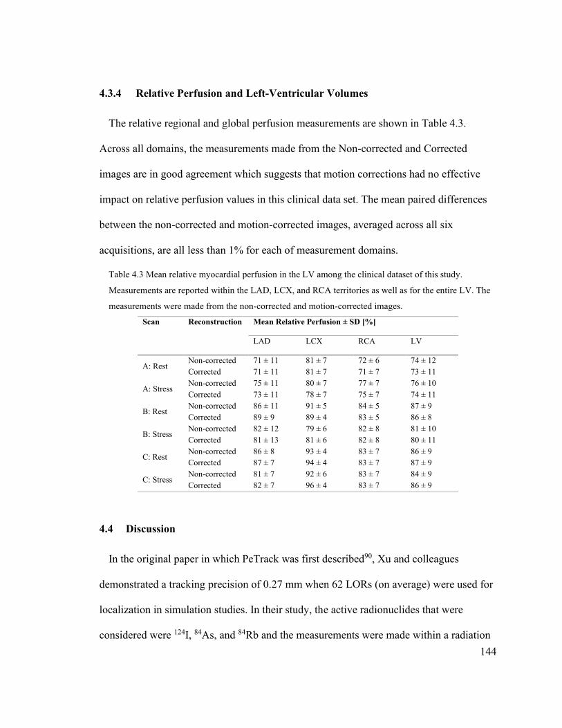
144

4.3.4 Relative Perfusion and Left-Ventricular Volumes

The relative regional and global perfusion measurements are shown in Table 4.3.

Across all domains, the measurements made from the Non-corrected and Corrected

images are in good agreement which suggests that motion corrections had no effective

impact on relative perfusion values in this clinical data set. The mean paired differences

between the non-corrected and motion-corrected images, averaged across all six

acquisitions, are all less than 1% for each of measurement domains.

Table 4.3 Mean relative myocardial perfusion in the LV among the clinical dataset of this study.

Measurements are reported within the LAD, LCX, and RCA territories as well as for the entire LV. The

measurements were made from the non-corrected and motion-corrected images.

Scan Reconstruction Mean Relative Perfusion ± SD [%]

LAD LCX RCA LV

A: Rest Non-corrected 71 ± 11 81 ± 7 72 ± 6 74 ± 12

Corrected 71 ± 11 81 ± 7 71 ± 7 73 ± 11

A: Stress Non-corrected 75 ± 11 80 ± 7 77 ± 7 76 ± 10

Corrected 73 ± 11 78 ± 7 75 ± 7 74 ± 11

B: Rest Non-corrected 86 ± 11 91 ± 5 84 ± 5 87 ± 9

Corrected 89 ± 9 89 ± 4 83 ± 5 86 ± 8

B: Stress Non-corrected 82 ± 12 79 ± 6 82 ± 8 81 ± 10

Corrected 81 ± 13 81 ± 6 82 ± 8 80 ± 11

C: Rest Non-corrected 86 ± 8 93 ± 4 83 ± 7 86 ± 9

Corrected 87 ± 7 94 ± 4 83 ± 7 87 ± 9

C: Stress Non-corrected 81 ± 7 92 ± 6 83 ± 7 84 ± 9

Corrected 82 ± 7 96 ± 4 83 ± 7 86 ± 9

4.4 Discussion

In the original paper in which PeTrack was first described90, Xu and colleagues

demonstrated a tracking precision of 0.27 mm when 62 LORs (on average) were used for

localization in simulation studies. In their study, the active radionuclides that were

considered were 124I, 84As, and 84Rb and the measurements were made within a radiation

145

therapy context using a custom detector system consisting of two pairs of position-

sensitive scintillating crystal arrays. While a meaningful comparison between the

tracking precision observed in this study to that of Xu et al. cannot be made, the stated

tracking precision of 0.27 mm serves as a useful benchmark. The tracking precision was

estimated in this work using the motion traces of the phantom experiments. From the

Reference acquisition where no motion existed the precision was estimated as the

standard deviation from the first 60 s (120 samples) of the acquisition. In the left-right,

anterior-posterior and inferior-superior directions, tracking precisions were 0.31 mm,

0.26 mm, and 0.25 mm, respectively. The mean number of LORs per tracking instance,

averaged across the first 60 s, was 124 ± 11. In the first reported use of PeTrack within

the context of PET, Chamberland and colleagues166 reported a 3D precision of 0.8 mm.

The addition in quadrature of the individual components stated above yields a 3D

precision estimate of 0.47 mm. From this it seems that the tracking precision achieved

within the present phantom experiments is in good agreement with previous studies of the

PeTrack tracking method. Qualitatively, the tracking precision of the left-right (or lateral)

component of the Diagonal motion case appears to exhibit reduced precision, particularly

in the first 60 seconds of the acquisition. Indeed, the tracking precision for this segment

of the motion was 0.76 mm, more than twice that observed for the reference acquisition.

The mean number of LORs per tracking instance within this time frame was 81 ± 10,

which based on previous PeTrack studies should generally provide sufficient tracking

quality. Nevertheless, the exact reason for the reduction in tracking precision for this

acquisition remains unclear.

146

In the Bland-Altman plot shown in Figure 4.7(B) a trend is apparent that suggests that

when the magnitude of the mean displacements increase, the image-based measurements

are low compared to those of PeTrack. This effect manifests as a negative slope among

the data points shown on this plot. The reason for this is most likely associated with

attenuation correction artifacts for the frames that deviate furthest from the reference

position, at which adequate attenuation correction was expected. This result is not

surprising as no motion correction was implemented for this dynamic reconstruction to

minimize CTAC artifacts.

In the original conference record publication167, the CNR measurements of the

phantom scans used a background VOI within the model LV blood pool, but this led to

confounding measurements as there was no tracer injected into this region. As a result, as

the initial injected activity within the LV decayed there was no similar decay within the

background region which reduced the relative improvement in CNR due to motion

correction. Therefore, the CNR measurements were repeated using a background VOI

that contained water in the body of the phantom in which a uniform activity distribution

existed. Nevertheless, only a single injection into the phantom was performed for the four

acquisitions that were performed. While the 18F-based tracer has a relatively long half-life

of 1.83 hours, non-negligible tracer decay occurred over the course of the experiment that

was not compensated for prior to comparing CNR values between the reference and

subsequent motion cases. In a simple model of a radioactive signal amid a lower activity

background, of the same radioisotope, the CNR can be shown to decay at half the rate of

this signal itself. An example of the model is shown in Figure 4.13 where the signal and

background are associated with the β+ decay of 18F. The solid curve of the figure

147

represents the activity of the signal region as a function of time, the dashed line

corresponds to the CNR (normalized to the initial value), and the markers indicate the

expected CNR at the start time of each of the phantom acquisitions with respect to the

start of the Reference scan. Simply due to decay, the CNR of the Axial, Lateral and

Diagonal acquisitions are reduced compared to the Reference by approximately 4%, 8%,

and 12%, respectively. These relative losses correspond to dominant proportions of the

reductions in CNR stated previously for the motion-corrected images. While these effects

apply equally to the non-corrected images, they represent a smaller fraction of the

measured losses.

Figure 4.13 Effect of radioactive decay between phantom acquisitions on CNR. The signal decay, CNR

and acquisition start times are indicated by the solid line, dashed line, and markers, respectively. All data

have been normalized to their respective initial value to focus on their relative changes over time.

In contrast to the relatively large increases in CNR observed for the phantom

experiment following motion correction, the effects of motion correction within the

clinical dataset are much less substantial. The primary reason for this is that the patients

148

in the clinical dataset were selected randomly and were not screened for patient motion.

The phantom experiments exhibited motion displacements up to approximately 20 mm in

magnitude. As a reference of scale, the typical LV wall thickness is roughly 10 mm.

Moreover, the phantom motion was persistent in moving away from the reference

location. In clinical studies, however, patient motion has been found to exhibit motion

that either non-returning or returning motion.142 The latter type of motion implies that a

displacement from the reference position is transient which mitigates the effects of

motion. Indeed, within this cohort the mean displacements (averaged across the

acquisition duration) were typically less than 1 mm. The root-mean-squared

displacements ranged from 1.3 – 4.7 mm but are not indicative of the changes in the

direction of motion throughout the acquisition. Thus, it appeared as though patient

motion was transient and, on average, the patients deviated only marginally from the

reference position. Due to the limited extent of motion within this group, the detection of

changes among the metrics indicated previously between Non-Corrected and Corrected

images was limited.

The maximal displacements, among all Cartesian directions, observed for each

acquisition indicated that the stress acquisitions had larger maximal displacements than

those of rest: 10.1 – 12.3 mm compared to 5.1 – 8.1 mm, respectively. These maximal

displacements agree with those reported previously by Hunter et al.82 The stress scans of

Patients B and C exhibited the highest maximal displacements, largely along the right-left

direction. Not surprisingly, it was for these two acquisitions that the largest changes in

LV thickness were observed between the non-corrected and motion-corrected images.

149

This effect was also mirrored by a substantial increase in CNR for Patient C, but not,

however, for the stress acquisition of Patient B.

The relative perfusion and LV volume measurements seemed quite insensitive to the

choice of non-corrected or motion-corrected image reconstructions. Across the LV, or

individual LV territories, the standard deviations ranged from 4% to 11%. It may be that

the intra-subject perfusion variation is sufficiently high to mask the effects of mild

motion. An effect of patient motion within cardiac PET imaging is to blur regions of

reduced uptake, which could correspond to disease, in such a way as to mask the severity

of the reduced perfusion. Within this cohort, as shown in Table 4.3, there did not appear

to be any cases of markedly reduced perfusion in a particular territory. While LV blood

pool volumes were shown to increase after applying motion correction, the changes were

relatively small compared to the Non-corrected volumes. In future work, the inclusion of

patients with suspected or confirmed coronary artery disease would be useful for

evaluating the potential of the motion correction approach for enhancing the perfusion

defects.

This method was designed to address whole-body patient motion, but it is not yet clear

how other types of motion could potentially limit the performance of the PeTrack motion

correction algorithm. In principle, severe respiratory motion (as measured with the

external marker) could give rise to motion triggers and thus confound the proposed body-

motion detection approach. The use of a sliding window smoothing kernel is expected to

limit the sensitivity of this approach to respiratory motion. As was shown in Chapter 3,

the IQR of the respiratory rates observed (roughly across all gating methods) ranged from

10 – 20 breaths/min. These rates correspond to breath periods in the range of 3 – 6 s. As

150

the sliding window span was 5 s, we expect that the respiratory signal of the marker will

be suppressed for most patients and most respiratory cycles. That said, future work

remains to demonstrate this assertion. Moreover, both whole-body and respiratory motion

could be characterized for each acquisition and dual body-respiratory motion correction

could be implemented.

4.5 Conclusions

In this study the feasibility of whole-body motion correction using 3D motion

information derived from tracking radioactive markers using the PeTrack algorithm was

demonstrated. The phantom experiments provided strong evidence that rigid whole-body

motion correction based on motion tracking with PeTrack can significantly reduce the

blurring artifacts associated with patient motion.

PeTrack was shown to exhibit 3D motion information of the marker during 13N-

ammonia cardiac perfusion PET studies that was in excellent agreement with image-

based measurements. Within this small sample of patients with limited motion, image

quality was not obviously degraded by motion artifacts and thus motion correction was

not found to improve image quality or have impact on relative perfusion measurements in

the LV. Future investigations are warranted to assess the impact that this motion

correction algorithm may have in the clinic, not only in static imaging but also dynamic

protocols where inter- and intra-frame patient motion need to be considered to improve

the precision of absolute blood flow quantification.

151

Chapter 5 Whole-Body Motion Correction for Absolute Blood Flow

Quantification

The content of this chapter represents an extension of the methods developed in

Chapter 4 in the context of dynamic myocardial perfusion imaging studies wherein

kinetic modelling is employed to calculate left-ventricular absolute blood flow. The work

described here has not been published or presented previously.

5.1 Motivation

Given the growing body of evidence that suggests that body motion should be

accounted for in cardiac PET/CT studies and given the observed limitations of frame-

wise correction methods, we sought to investigate two data-driven methods for motion

correction prior to kinetic modelling in cardiac perfusion PET/CT studies to estimate

absolute myocardial blood flow (MBF). Refer to Section 1.3.3 for details and definitions

regarding MBF estimation. In the proposed framework we exploit the high temporal

resolution of data-driven tracking methods to detect intra- and inter-frame motion.

Additionally, we also designed our MC approach to address the problem of mis-

registration between PET emission data and attenuation correction data which is derived

from a static CT acquisition. Two data-driven motion tracking/detection systems were

employed and compared. These consist of the positron emission tracking (PeTrack)

algorithm167 and the centroid of distribution (COD) method.119 Both methods use only

list-mode data from the PET scanner to generate a motion tracking signal. They differ,

however, in that the former tracks the motion of low-activity point sources placed on the

patient while the latter uses only emission data from the radiotracer. While other data-

152

driven motion tracking approaches have been proposed or demonstrated to detect body

motion117,171, they are technically similar to the COD approach and were not

implemented for this study.

5.2 Methods

5.2.1 Centroid of Distribution (COD) Motion Tracking

The COD algorithm described in the work of Lu and colleagues119 was implemented

for this study with only minor modification. This data-driven approach to tracking patient

motion is based on calculating the mean position of the most likely annihilation (MLA)

points (calculated from TOF) from a set of LORs belonging to a specific time interval.

This calculation is repeated for each adjacent time window throughout the acquisitions to

derive a 3D motion trace of the centroid. This technique is advantageous in that it relies

only on the tracer activity administered to a patient and is relatively fast to compute as it

does not employ iterative methods. Generating a motion trace from list mode data

typically required 1 minute of processing time using a standard desktop workstation.

In its original implementation for tracking body motion, all LORs acquired by the PET

system were used for tracking. Lu and colleagues119 developed this method using animal

and human PET studies which considered several different 18F-based tracers with various

targets within the torso. Since the imaging target of this work is the heart, LORs that were

unlikely to have originated within a cubic volume of interest (VOI) centered about the

heart were excluded from the centroid calculation. Additionally, the time interval used for

each centroid calculation was fixed at 1 second in its original implementation. In this

study, a tracking interval of 0.5 s was used to match that which is used for PeTrack.

153

The VOIs were created manually for each acquisition included in this study using a

custom graphic user interface developed using MATLAB (MathWorks®, Natick,

Massachusetts, USA). The VOIs were drawn on static uptake images where the

myocardium has a relatively high contrast compared to the extracardiac space. The VOIs

were intentionally drawn larger than the heart to allow for motion of the heart within that

space. LORs in any time interval were initially excluded if their MLA points did not fall

within the VOI. A one-dimensional probability density function (PDF) was used to

describe the distribution of the possible annihilation location along a LOR. The PDF was

integrated within the limits set by its intersection points of the VOI to determine the

probability that the LOR originated from within the VOI. The PDF was assumed to be a

Gaussian function centered at the MLA point with a FWHM of 80 mm, to match the TOF

resolution of the Discovery 690 PET/CT system that was used to acquire the data (see

Table 1.2). The probability cut-off was chosen to be 10% after evaluating the COD

motion traces using various values ranging from 0 – 50%. The cut-off of 10% was shown

to provide a reasonable balance between signal noise and accuracy. This LOR rejection

method is illustrated in Figure 5.1. The phantom studies described in Chapter 4 were used

for this assessment. Examples of these traces are provided in the results, Section 5.3.

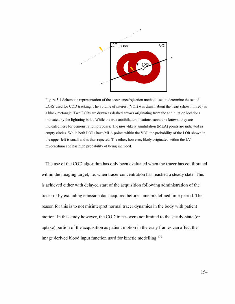
154

Figure 5.1 Schematic representation of the acceptance/rejection method used to determine the set of

LORs used for COD tracking. The volume of interest (VOI) was drawn about the heart (shown in red) as

a black rectangle. Two LORs are drawn as dashed arrows originating from the annihilation locations

indicated by the lightning bolts. While the true annihilation locations cannot be known, they are

indicated here for demonstration purposes. The most-likely annihilation (MLA) points are indicated as

empty circles. While both LORs have MLA points within the VOI, the probability of the LOR shown in

the upper left is small and is thus rejected. The other, however, likely originated within the LV

myocardium and has high probability of being included.

The use of the COD algorithm has only been evaluated when the tracer has equilibrated

within the imaging target, i.e. when tracer concentration has reached a steady state. This

is achieved either with delayed start of the acquisition following administration of the

tracer or by excluding emission data acquired before some predefined time-period. The

reason for this is to not misinterpret normal tracer dynamics in the body with patient

motion. In this study however, the COD traces were not limited to the steady-state (or

uptake) portion of the acquisition as patient motion in the early frames can affect the

image derived blood input function used for kinetic modelling.172

155

5.2.2 Whole-Body Motion Detection

A novel motion detection algorithm was developed for this study which was applied to

both PeTrack and COD motion traces. It was designed to detect and record instances

along the motion trace which corresponded to patient motion. These instances of motion

are referred to hereafter as body motion triggers, or triggers. Several different approaches

were developed for this purpose, which employed either physical threshold, signal

processing techniques or statistical arguments to indicated that a relatively significant

change in the position of the motion trace has occurred. They were developed with the

use of the phantom studies described in Chapter 4 where the motion triggers were known

a priori. The final method was chosen as that which indicated the best agreement between

the PeTrack and COD tracking approaches.

The selected approach is a graphical method which is closely related to measurements

of the velocity components of each 1D component on the motion trace. In this approach

the position and time were treated as generalized coordinates. A linear fit of these the

position and time coordinates was performed on each component within a 20 s sliding

window. The elevation angle of the fitted line, which represents the degree of change in

the position, was measured between the vector normal to the line and the positive vertical

direction, i.e. the generalized vector which has components in the time and position

domains of 0 and 1, respectively. The spatial and temporal units of the motion traces

were millimeters and seconds, respectively. This approach is similar to imposing

thresholds on the average velocity of each component computed over the duration of the

sliding window. Figure 5.2 provides an example 1D motion trace on which the normal

vectors are overlaid for each sliding window position.

156

Figure 5.2 Example motion detection where the processed trace is depicted along the calculated normal

vector. Only the anterior-posterior component of the motion trace is shown. The time domain is split to

isolate two body motion triggers (dashed vertical lines) that were identified at 103 s and 238 s. The

trigger at 103 s (trigger ‘a’) corresponds to change in position with a relatively steep gradient, whereas

the trigger at 238 s (trigger ‘b’) corresponds to a low gradient, steady change in position. The local linear

fits at each of the triggers are shown by red dashed lines. The angles between the generalized vectors and

the vertical direction are indicated as for each trigger. Note that the length of the arrows is arbitrary as

they are scaled automatically to ensure the arrow tips do not cross adjacent arrows.

The window was incremented with a step size of 0.5 seconds until it reached the end of

the acquisition. When motion was detected, a body motion trigger was inserted at the

mean temporal position of the window. Motion was considered to be present if either of

the following criteria were met: the instantaneous deflection angle exceeded a threshold

(θ1), or when the accumulated deflection angle exceeded a threshold (θ2). Note that the

accumulated deflection angle was initialized at 0º and was modified by each time

window; it was reset to 0º if it reached θ2 and accumulation began again. These two

events correspond to rapid changes and gradual drifts of the position in each direction of

motion. The two thresholds were initially selected by assessment of the performance of

both tracking methods to correctly identify triggers in the phantom studies. The phantom-

derived deflection thresholds (θ1, θ2) were set as 15º and 90º, respectively. Note that θ1 =

157

15º is equivalent to an average velocity of 0.27 mm/s over the sliding window duration,

whereas the θ2 = 90º could be reached, for example, if an average velocity of 0.016 mm/s

were maintained over a 70 s period.

The phantom-derived thresholds were ultimately found to be unsuitable for human

studies due to the abruptness and magnitude of the motion in the phantom studies. A

small set of studies which exhibited either abrupt and/or gradual motion, as observed in

the motion traces, were used to determine the deflection thresholds for human studies.

The instantaneous deflection threshold (θ1) was adjusted to be 24º (or 0.45 mm/s),

although in practice only gradual motion (accumulated deflection ≥ 90º) appeared to be

relevant.

The motion traces were filtered at the outset to make motion detection less susceptible

to noise. The signals were convolved with an averaging kernel with a span of 5 seconds.

An additional low pass filter was employed for the human studies, to reduce the impact of

respiratory motion on body-motion detection; the cut off frequency was chosen as 0.17

Hz, which removes signal components with periods less than 6 seconds.

Motion triggers were produced independently within each dimension of the 3D motion

traces. Triggers associated with each direction of motion were concatenated into a single

set. Triggers from different directions of motion that agreed with each other were

merged. In the event that a pair of triggers were separated by 5 seconds or less, only the

first of the two was kept. Triggers that were identified in the first 10 seconds of an

acquisition were ignored as in some cases signal artifacts were present as a result of the

low pass filter due to the finite dataset. The first 10 seconds of an acquisition, which

158

immediately followed tracer administration, was observed to be very count deficient and

so ignoring triggers in this window was expected to be of little to no effect.

5.2.3 Motion Estimation and Correction

Motion correction was performed in a two-step process. Patient motion was first

estimated and subsequently incorporated into the reconstruction workflow to correct it. In

the following we describe the motion correction framework and then the motion

estimation approaches.

The original list-mode data were divided into a set of ‘motion frames’ that was

determined by a combination of the body-motion triggers (tbm) identified in the motion

detection step and the start times of the dynamic frames used for clinical reconstructions.

Body-motion triggers were inserted into the list of the frame start times of the dynamic

series. When a body-motion trigger was within 2.5 seconds of a dynamic frame start

point, the start point was adjusted to match the trigger. If the trigger was further than 2.5

seconds from the nearest start point a new frame was created which began at the trigger

and ended at the earlier of either the next body-motion trigger or dynamic frame start

time. The original dynamic frame definitions are retained in the workflow and are

considered as parents to all motion frame children that exist within their duration. The

way in which the motion frames are combined to return to the original parent dynamic

frames is described later in the section.

Two motion estimation methods were considered for use in this study to derive the

transformation parameters. In the first approach, motion estimates were based on the

direct use of the 3D displacements determined from the motion tracking results. The

159

frame-wise displacement for each motion frame was calculated from the motion trace

displacement with respect to the reference position averaged across the frame duration.

In the second approach, the transformation matrices were produced from a 6D rigid

image registration of non-attenuation corrected images. Non-attenuation corrected

images were used to avoid the propagation of potential PET/CT mis-alignment artifacts

into registration errors.119 Given that the activity distribution is not fixed for dynamic

PET acquisitions that commence with tracer administration, a sequential image

registration approach was employed. This approach is based on the assumption that the

adjacent frames in a dynamic acquisition are more similar than a pair of temporally

distant images and thus registration should be more accurate. To make this explanation

more explicit, consider a dynamic reconstruction that contains n frames and the reference

was chosen as the nth frame. Then in a sequential registration, the first frame is registered

to the second, the second to the third, and so on, until the (n-1)th was registered to nth,

reference frame. To align the first frame to the reference, one would need to apply all (n-

1) transformations or compose each and apply a single transformation. Sequential

registration for dynamic images where the tracer distribution has not equilibrated has

been reported elsewhere.119,173

In this work, the reference images were selected as the frame that occurred later than 2

minutes after the acquisition, with greatest number of counts. This time window

corresponds to images with myocardial uptake and clearance of the activity in the blood

pool. This reference image was chosen to help ensure good alignment with the CT

images used for attenuation correction which were manually aligned to the static uptake

images by technologists at the time of the original PET acquisitions. The frame in the

160

uptake window with the greatest number of counts was expected to be most like the static

images.

Image registrations were performed using the Elastix software package.174 Mutual

information was chosen as similarity metric between the moving and references images.

A multi-resolution registration using a gradient descent optimization algorithm was used

to estimate the transformation parameters. More complex motion models such as affine

and non-rigid were also initially considered for use but did not provide robust motion

estimates. This was observed during registration of the motion frames of the phantom

scans described in Chapter 4, where the manually applied motion was well known. In

these tests, non-rigid motion models were not able to reproduce the expected translations.

Regarding the choice of similarity metric, mutual information175,176 evaluates the entropy

in the joint distribution of grey-level values observed in two images. With respect to

registration, it is hypothesized that the mutual information is maximized when the like

structures are aligned as the joint histogram exhibits the highest level of organization, or

lowest entropy. Mutual information serves as a useful similarity metric between images

that do not have similar intensity and has thus been used for image registration between

different modalities177,178 or for dynamic data sets.119,179 There were numerous user-

specified input parameters that can impact the outcome of the registrations results which

related to the choice of transformation model, similarity metric, interpolation, and

optimization. Following the recommendations of the user documentation, many default

parameters were specified. The input parameter file that was used to specify all

nondefault parameters is included as Appendix B.

161

Prior to reconstruction, the static CT image used for attenuation correction was

transformed using the inverse of the transformation matrices used to align the PET

motion frames to achieve accurate attenuation correction of each reconstructed frame.

Following the reconstruction of the set of motion frames, each were aligned with the

reference frame by applying the forward transformation matrices. They were

subsequently combined into the original dynamic frame sequence by computing the

weighted average of any new motion frames which fell within the duration of an original

dynamic frame to form the final, motion-corrected dynamic series. The weights used in

the weighted average corresponded to the relative number of coincidence counts

observed in each frame compared to the total in the entire list mode data set. As an

example, consider an acquisition which took place over 360 s with dynamic frames of

120 s duration beginning at 0, 120, and 240 s. If body-motion triggers were detected at 30

and 90 s, it follows that the parent frame beginning at 0 s would be divided into three

motion frames (with start times of 0, 30, and 90 s). In total, 5 motion frames would be

reconstructed but the motion frames starting at 0, 30, and 90 s would be combined via

weighted averaging to produce the motion corrected parent frame beginning at 0 s and

ending at 120 s. The remaining parent frames would also be motion corrected but would

not require recombination.

Note that weights based on counts help to suppress noise in the average frame, but this

could come at the expense introducing bias in the pixel values when tracer decay between

motion frames was relatively significant. Alternatively, weights based on frame duration

would be more accurate, but the added noise could make image registration more

challenging. The need for reconstruction of individual motion frames was a limitation of

162

the vendor reconstruction software as it was not possible to incorporate motion

estimations directly into the reconstruction algorithm as has been described in other work

related to body motion correction.119,180

5.2.4 Clinical Dataset

To evaluate our proposed MC framework and compare these two data-driven motion

tracking approaches a combination of phantom and clinical scans were used. All data

were acquired at the University of Ottawa Heart Institute, Ottawa, on a GE Discovery

690 scanner27 (Waukesha, WI). The anthropomorphic torso phantom acquisitions that

were described in Section 4.2.2 were used in this study to develop the motion detection

method and also for validation of the implementation of the Elastix image-registration

software.

The clinical data consisted of 9 patients that underwent 13N-ammonia (NH3) or 82Rb

myocardial perfusion studies at rest and/or stress. In total 17 acquisitions were included,

five (N = 5) 13NH3 acquisitions from three patients, and twelve (N = 12) 82Rb acquisitions

from six patients. The 6 patients that underwent 82Rb perfusion studies are referred to as

patients ‘A’ – ‘F’, whereas the 3 patients that underwent 13NH3 perfusion studies are

referred to as patients ‘G’ – ‘I’. Note that some of the data sets included here were used

previously in Chapter 4. Patients H and I in this chapter corresponds to patients B and C,

respectively, in Chapter 4. Acquisitions were 20 minutes and 8 minutes in duration for

13NH3 and 82Rb studies, respectively. Physiologic stress was induced using intravenous

injection of dipyridamole. The dose protocols at our institution for these studies are 3

MBq/kg and 9 MBq/kg for 13NH3 and 82Rb, respectively. Low dose CT scans were

163

acquired prior to each PET acquisition for attenuation correction. In our clinic

technologists perform a manual 3D co-registration between an initial static reconstruction

and the CT image used for attenuation correction. These translations were used in this

work to define the reference position of the patient that provides good

emission/transmission overlap.

In all cases image reconstructions were performed offline using research reconstruction

software supplied by the vendor. An OSEM algorithm was used (4 iterations and 24

subsets) which included corrections for random and scatter coincidence events, and

attenuation correction. For each acquisition included in this study five types of dynamic

image reconstruction were considered: dynamic without motion correction (NMC);

motion correction using PeTrack (PT); and motion correction using COD (CD). Note that

two approaches of motion estimation were employed for both PeTrack and COD. The

resulting images correspond to PT3D, PT6D, CD3D, and CD6D where the label ‘3D’

corresponds 3D motion estimation using the motion trace directly and ‘6D’ corresponds

to the use of 6D rigid image registration for motion estimation. The dynamic frames were

pre-defined based on the standard imaging protocols used at UOHI. For 82Rb perfusion

studies they consisted of 14 frames (including the first 6 minutes of each acquisition)

configured as 10 × 10 s frames, 1 × 30 s frame, 1 × 60 s frame, and 1 × 120 s frame. The

13NH3 perfusion studies consisted of 17 frames configured as 9 × 10 s frames, 3 × 30 s

frames, 1 × 60 s frame, 1 × 120 s frame, 1 × 240 s frame, and 2 × 300 s frames.

The visual motion assessment of the NMC images was performed using a 3D DICOM

image viewer which displays transverse, coronal, and sagittal views simultaneously.

Motion of the myocardium and the radioactive fiducial marker were both considered.

164

Additionally, it was noted whether patient motion exhibited returning behaviour, i.e. was

a given change on patient position followed by a another with similar magnitude but

reversed direction.

5.2.5 Verification of COD Tracking and Image Registration Methods

Initial testing was performed to verify that the COD tracking method was implemented

correctly and determine the probability threshold associated with the exclusion of LORs

from the cardiac VOI. The COD traces were initially produced for the phantom

acquisitions described in Chapter 4. This test was largely qualitative to confirm that COD

tracking could accurately estimate the translations that were manually applied to the

phantom during the reference (no motion) and axial motion acquisitions. To determine a

suitable probability threshold associated with excluding LORs from the cardiac VOI,

COD tracking was performed multiple times for a range of probability cut-off values and

the effect on mean and standard deviations of the observed translations was measured.

The best probability cut-off was chosen as that which exhibited the best trade-off

between noise and accuracy.

The image registration software was also configured and tested using the phantom

acquisitions. The phantom acquisition that contained only axial translations was used to

assess the quality of the image registration’s estimates. Given the high precision that was

demonstrated by PeTrack to measure the motion in this acquisition (see Section 4.3.1), its

recorded translations were used for comparison against those from image registration.

Each of the frames corresponding to one of the five phantom positions was registered

directly to a reference frame and the translation between each with the reference frame

165

were recorded. This process was repeated five times with each motion frame serving as

the reference frame in turn. The registration accuracy was measured as the root mean

square error (RMSEreg) between the translation indicated by PeTrack with those from the

registration among all five trials. The variability of the registration process due to

changes in the reference frame was considered as the precision of the registration. The

translation values for each trial were shifted as though the first frame was the reference.

The precision of the registration was measured as the mean absolute difference (MAD) of

the shifted translation of each motion frame with the first. The definitions of the RMSEreg

(accuracy) and MAD (precision) are defined as

𝑅𝑀𝑆𝐸𝑟𝑒𝑔 = √1

𝑁𝐹𝑁𝑇∑ ∑(∆𝑧𝑖𝑗

𝐼𝑅 − ∆𝑧𝑖𝑗𝑃𝑇)

2

𝑁𝑇

𝑗=1

𝑁𝐹

𝑖=1

Eq. 0.1

𝑀𝐴𝐷 =

∑ ∑ |∆𝑧𝑖𝑗𝐼𝑅′ − ∆𝑧𝑖1

𝐼𝑅′|𝑁𝑇𝑗=2

𝑁𝐹𝑖=2

(𝑁𝐹 − 1)(𝑁𝑇 − 1)

Eq. 0.2

where 𝑁𝐹 = 5 and 𝑁𝑇 = 5 represent the number of frames and trials, respectively. The

translation between the ith frame with the reference frame of the jth trial is denoted as

∆𝑧𝑖𝑗𝐼𝑅 and ∆𝑧𝑖𝑗

𝑃𝑇, for the image registration and PeTrack estimates, respectively. Lastly,

∆𝑧𝑖𝑗𝐼𝑅′ represents ∆𝑧𝑖𝑗

𝐼𝑅 − ∆𝑧1𝑗𝐼𝑅, the estimated translation between frame i and the first

frame, calculated as the difference between the translations of the two frames to the

reference frame with trial j as reference. Note that in the MAD calculation, the indices

start at 2 as ∆𝑧𝑖𝑗𝐼𝑅′≡ 0 for the first frame (i = 1) for all trials (j).

As the phantom acquisitions did not contain rotational motion, image rotations were

artificially introduced to the first frame of the axial motion case to ensure that the

166

registration could estimate rotations. Image rotations of ±5º, ±10º, and ±20º about z-axis

(longitudinal axis of the PET field of view) were performed. The root mean square error

between the known and estimated rotations was determined as a measure of the accuracy.

The phantom acquisitions were not suitable for testing the effect of tracer kinetics and

tracer decay, as they were injected with 18F-FDG and the tracer distribution within the

phantom was static.

5.2.6 Absolute Blood Flow Quantification and Figures of Merit

Blood flow quantification was performed using the FlowQuant© (version 2.7)

software package which was developed at the University of Ottawa Heart Institute.159

This research tool is a graphical-user-interface application which permits automated

analysis of cardiac PET images and includes kinetic modelling workflows. For the

acquisitions which used 82Rb a one-tissue compartment model159 was employed on the

first 6 minutes of data.181 For the 13NH3 studies, the two-tissue compartment model was

used182 which used the entire 20-minute dynamic acquisition. In both cases, the kinetic

models were constrained such that the tissue-to-blood ratio of activity concentration was

fixed. At equilibrium, this ratio is equivalent to the ratio of K1 to k2 kinetic model

parameters, as defined in Section 1.3.3. The specific value was determined based on the

unconstrained model parameters determined in a region of normal uptake, i.e. with a

relative uptake greater than 80%. This constraint was shown previously to improve inter-

operator repeatability of blood flow measurements using FlowQuant.159

The tissue and blood regions are defined using an average uptake image which used all

frames in the ranges of 1.5 – 6 minutes and 2.5 – 20 minutes for 82Rb and 13NH3,

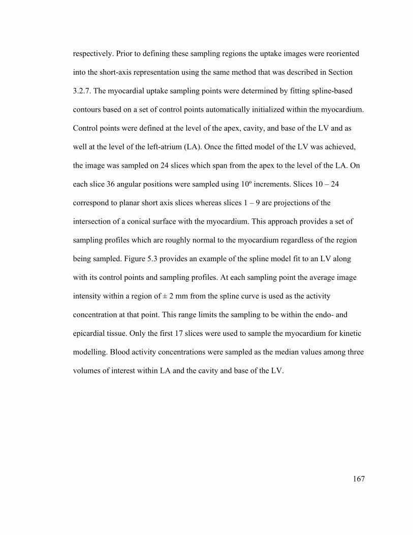
167

respectively. Prior to defining these sampling regions the uptake images were reoriented

into the short-axis representation using the same method that was described in Section

3.2.7. The myocardial uptake sampling points were determined by fitting spline-based

contours based on a set of control points automatically initialized within the myocardium.

Control points were defined at the level of the apex, cavity, and base of the LV and as

well at the level of the left-atrium (LA). Once the fitted model of the LV was achieved,

the image was sampled on 24 slices which span from the apex to the level of the LA. On

each slice 36 angular positions were sampled using 10º increments. Slices 10 – 24

correspond to planar short axis slices whereas slices 1 – 9 are projections of the

intersection of a conical surface with the myocardium. This approach provides a set of

sampling profiles which are roughly normal to the myocardium regardless of the region

being sampled. Figure 5.3 provides an example of the spline model fit to an LV along

with its control points and sampling profiles. At each sampling point the average image

intensity within a region of ± 2 mm from the spline curve is used as the activity

concentration at that point. This range limits the sampling to be within the endo- and

epicardial tissue. Only the first 17 slices were used to sample the myocardium for kinetic

modelling. Blood activity concentrations were sampled as the median values among three

volumes of interest within LA and the cavity and base of the LV.

168

Figure 5.3 Demonstration of the FlowQuant LV sampling method. The spline fit, shown as a solid red

curve, and its control points, empty circles, are shown on horizontal long-axis (HLA) and vertical-long

axis (VLA) images. The blood sampling volumes of interest are indicated as regions bounded by a solid

black border with the labels A (atrium), B (base), and C (cavity). Dashed lines represent the profiles

along which the myocardium is sampled. Note that the apical slices which appear to fan outward are

defined by conical surfaces which intersect the myocardium; all other slices are planar short-axis slices.

The red dashed line additionally indicates the basal extent of the LV used for myocardial sampling.

The FlowQuant GUI permits opportunities for manual intervention if the automatic

sampling tool failed but this was generally not needed. Manual intervention was required

for one 13NH3 acquisition where the spline fit was hindered by reduced uptake in the

apical anterior region as well as by extra-cardiac uptake in the left lung.

As described previously in Section 2.1, patient motion can lead to reduced accuracy of

myocardial blood flow quantification. In human studies, however, the motion-free flow

values are not known, and so blood flow alone is insufficient to identify and characterize

the effect of patient motion on dynamic cardiac PET studies. Other metrics related to the

goodness-of-fit of the myocardial TACs77, e.g. root-mean-square errors (RMSETAC) and

coefficient of determination (R2), and voxel-wise uncertainty of kinetic model parameters

169

like MBF183 (or K1) and total blood volume184 (TBV) have been proposed elsewhere and

were adopted for this work. Hereafter, the uncertainty of MBF and TBV will be referred

to as FlowSD and TBVSD, respectively. These are estimated from a non-linear fitting

procedure and are based on the sensitivity of the cost function to the fit parameters. In

the presence of motion, one would expect to observe higher variance (worse precision) in

kinetic model parameters as well as poorer goodness-of-fit of the TACs. The

myocardium goodness-of-fit measures reflect the agreement between the image-based

(measured) and model-derived (estimated) myocardial activity concentrations among all

time points. Recall that the measured and modelled myocardium TACs were defined

previously in Section 1.3.3 and are represented as 𝐶𝑚(𝑡) and ��𝑚(𝑡), respectively.

Definitions of the RMSETAC and R2 goodness-of-fit measures are provided below, where

𝑦𝑖 and 𝑓𝑖 represent the ith measured and regressed TAC values, and 𝑁 is the number of

data points on the TAC (or number of dynamic frames included in the kinetic model).

Additionally, 𝑆𝑆𝑟𝑒𝑠 and 𝑆𝑆𝑡𝑜𝑡 represent the residual sum-of-squares between the

measures and regressed values and the total sum-of-squares of the measures data,

respectively. FlowQuant calculates these metrics on a voxel-by-voxel basis during kinetic

modelling.

𝑅𝑀𝑆𝐸 = √

1

𝑁∑(𝑦𝑖 − 𝑓𝑖)2

𝑖

Eq. 0.3

𝑅2 ≡ 1 −

𝑆𝑆𝑟𝑒𝑠

𝑆𝑆𝑡𝑜𝑡= 1 −

∑ (𝑦𝑖 − 𝑓𝑖)2𝑖

∑ (𝑦𝑖 − ��)2𝑖

Eq. 0.4

170

5.3 Results

5.3.1 Verification of COD Tracking

The no-motion phantom acquisition was considered first. As the phantom did not move

during this acquisition any change fluctuation in the COD motion trace would indicate

either a mistake in the implementation or the susceptibility of the method to noise in its

signal. The COD tracking results for the reference phantom acquisitions are shown in

Figure 5.4. Figure 5.4(A) shows the example motion trace where the LOR probability

cut-off, or “pCut”, was 0.0. Figure 5.4(B) and (C) show the mean and standard deviations

of each dimension of the centroid position as a function of pCut. COD tracking for this

acquisition provided a consistent representation of the mean position regardless of the

choice of pCut. The standard deviation of each component of the position demonstrated

an exponential relationship with the choice of pCut indicating that the signal noise level

was strongly affected by the severity of the exclusion criteria of LORs used for COD

tracking.

The COD traces for the various values pCut were also examined for the phantom

acquisition where axial motion was included; the inferior-superior components for the

subset of the pCut values are plotted along with that from the PeTrack trace in Figure 5.5.

The most notable aspect of this comparison is the limited extent of motion observed using

COD tracking compared to PeTrack. The magnitude of displacements reported by COD

tracking were roughly 20% of that measured using PeTrack. The reason for this effect is

suspected to be associated with spatial dependence of the sensitivity of the PET system as

well as the presence of scattered coincidence events. When the phantom acquisition

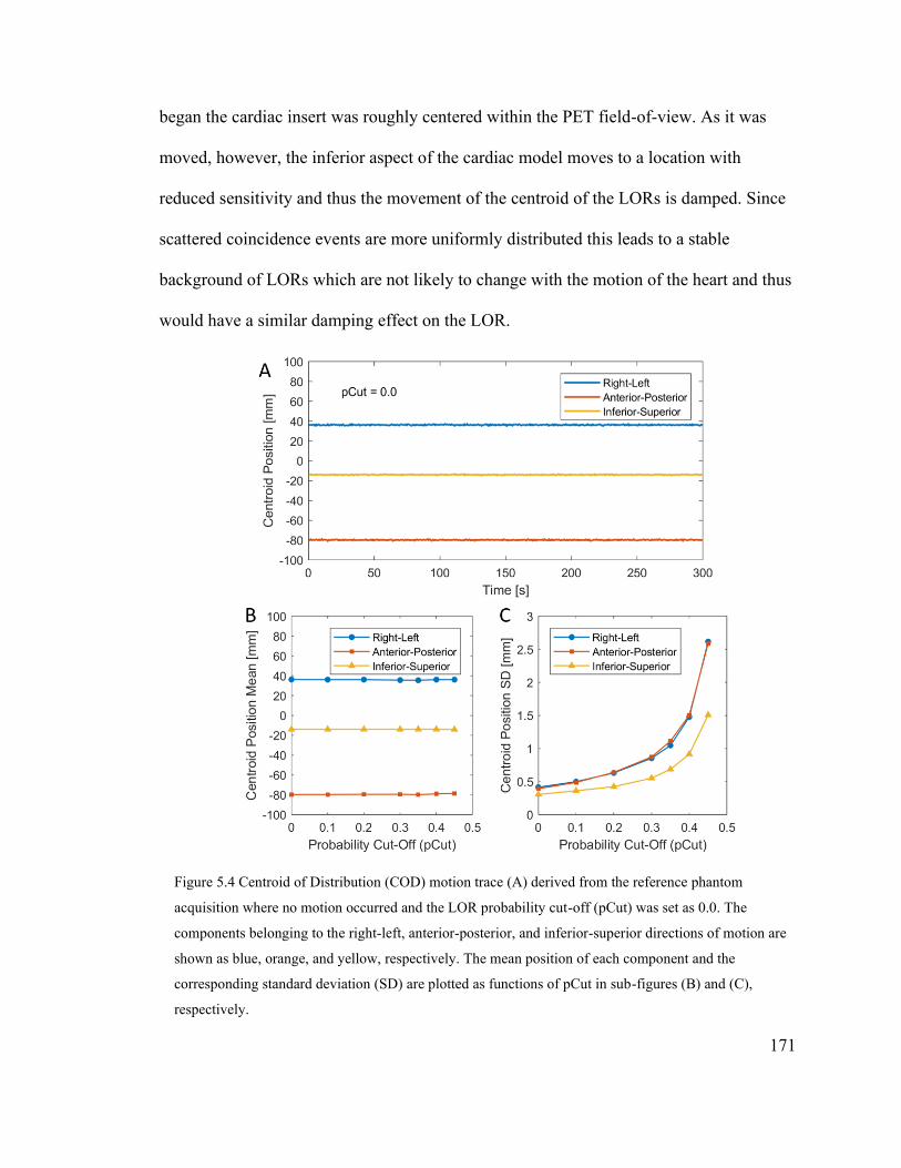
171

began the cardiac insert was roughly centered within the PET field-of-view. As it was

moved, however, the inferior aspect of the cardiac model moves to a location with

reduced sensitivity and thus the movement of the centroid of the LORs is damped. Since

scattered coincidence events are more uniformly distributed this leads to a stable

background of LORs which are not likely to change with the motion of the heart and thus

would have a similar damping effect on the LOR.

Figure 5.4 Centroid of Distribution (COD) motion trace (A) derived from the reference phantom

acquisition where no motion occurred and the LOR probability cut-off (pCut) was set as 0.0. The

components belonging to the right-left, anterior-posterior, and inferior-superior directions of motion are

shown as blue, orange, and yellow, respectively. The mean position of each component and the

corresponding standard deviation (SD) are plotted as functions of pCut in sub-figures (B) and (C),

respectively.

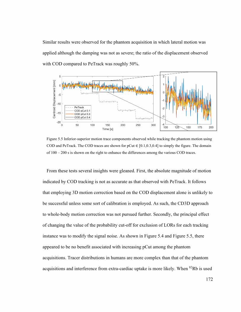
172

Similar results were observed for the phantom acquisition in which lateral motion was

applied although the damping was not as severe; the ratio of the displacement observed

with COD compared to PeTrack was roughly 50%.

Figure 5.5 Inferior-superior motion trace components observed while tracking the phantom motion using

COD and PeTrack. The COD traces are shown for pCut ∈ [0.1,0.3,0.4] to simply the figure. The domain

of 100 – 200 s is shown on the right to enhance the differences among the various COD traces.

From these tests several insights were gleaned. First, the absolute magnitude of motion

indicated by COD tracking is not as accurate as that observed with PeTrack. It follows

that employing 3D motion correction based on the COD displacement alone is unlikely to

be successful unless some sort of calibration is employed. As such, the CD3D approach

to whole-body motion correction was not pursued further. Secondly, the principal effect

of changing the value of the probability cut-off for exclusion of LORs for each tracking

instance was to modify the signal noise. As shown in Figure 5.4 and Figure 5.5, there

appeared to be no benefit associated with increasing pCut among the phantom

acquisitions. Tracer distributions in humans are more complex than that of the phantom

acquisitions and interference from extra-cardiac uptake is more likely. When 82Rb is used

173

uptake in the stomach wall and/or spleen is common185,186 whereas when 13NH3 is used,

uptake in the lung73 and pancreas187 is expected. It follows that pCut = 0.1 was used when

COD tracking was applied to the human acquisitions.

5.3.2 Verification of the Image Registration Method

The phantom acquisition in which axial motion was applied was used once more to

validate the image registration method. The RMSEreg of the inferior-superior inter-frame

translation between registration and PeTrack was found to be 1.2 mm. The MAD

associated with varying the reference frame of the registration was 1.5 mm. Together,

these metrics demonstrated that the motion estimation using image registration of these

phantom acquisitions was in good agreement with an independent approach: PeTrack,

and that the method was self-consistent and showed a small overall variability associated

with changes in the reference frame. The RMSEreg associated with rotations which ranged

from 5º – 20º about the longitudinal axis was 0.008º. Since the target and moving images

of this test were identical, save for the rotations imposed on them, this test simply

indicates that the registration algorithm could account for rotations and does not truly

represent its accuracy when applied to unique dynamic frames. This suggests that the

registration method was correctly initialized with reasonable parameter choices. It is

worth re-iterating that these tests could not assess the usefulness of the registration

method when a time-varying tracer distribution is present, as is the case in dynamic

perfusion studies performed on the patient cohort.

174

5.3.3 Evaluation of the Body-Motion Detection and Estimation Methods

As a final assessment of the motion correction workflow, motion-correction

reconstructions were performed for the phantom acquisition in which axial motion was

applied. Motion triggers were produced from both PeTrack and COD motion traces and

image registration was used for motion estimation, i.e. PT6D and CD6D motion

correction methods were employed. The two motion traces and their corresponding

triggers are shown in Figure 5.6.

Figure 5.6 Inferior-superior component of the motion traces of PeTrack (gray) and COD (yellow) for the

axial motion phantom acquisition. The triggers (tbm) identified for each trace are also shown as dashed

lines; they are colour-matched with the trace to which they belong. Due to the limited ability of COD to

estimate motion, the trigger corresponding to the first change in position near 60 s was not detected.

The motion detection algorithm was designed such that PeTrack and COD showed

produced comparable results during the task of identifying the instance of motion within

the phantom acquisitions. Perfect agreement could not be achieved given the difference

in scale of the two traces. The most notable difference is that the first transition around 60

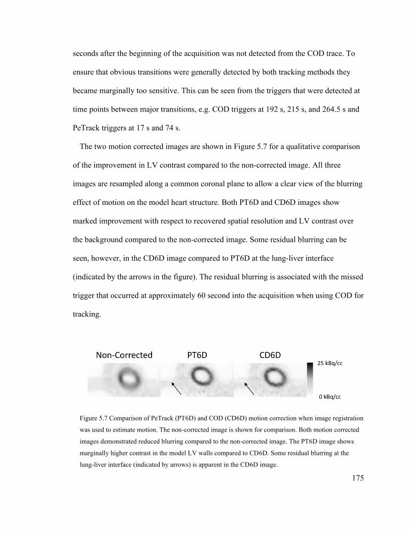
175

seconds after the beginning of the acquisition was not detected from the COD trace. To

ensure that obvious transitions were generally detected by both tracking methods they

became marginally too sensitive. This can be seen from the triggers that were detected at

time points between major transitions, e.g. COD triggers at 192 s, 215 s, and 264.5 s and

PeTrack triggers at 17 s and 74 s.

The two motion corrected images are shown in Figure 5.7 for a qualitative comparison

of the improvement in LV contrast compared to the non-corrected image. All three

images are resampled along a common coronal plane to allow a clear view of the blurring

effect of motion on the model heart structure. Both PT6D and CD6D images show

marked improvement with respect to recovered spatial resolution and LV contrast over

the background compared to the non-corrected image. Some residual blurring can be

seen, however, in the CD6D image compared to PT6D at the lung-liver interface

(indicated by the arrows in the figure). The residual blurring is associated with the missed

trigger that occurred at approximately 60 second into the acquisition when using COD for

tracking.

Figure 5.7 Comparison of PeTrack (PT6D) and COD (CD6D) motion correction when image registration

was used to estimate motion. The non-corrected image is shown for comparison. Both motion corrected

images demonstrated reduced blurring compared to the non-corrected image. The PT6D image shows

marginally higher contrast in the model LV walls compared to CD6D. Some residual blurring at the

lung-liver interface (indicated by arrows) is apparent in the CD6D image.

176

5.3.4 Sensitivity of Kinetic Modelling Quality Metrics to Motion

The reconstructed dynamic image series (NMC) were visually inspected to assess the

extent of motion in each of the 17 acquisitions. Of those, 4 were identified as severe

motion cases; they exhibited translational motion ≥ 6 mm. The remaining acquisitions

exhibited no motion or very minor motion, i.e. translations < 3 mm, and are referred to

here as mild motion cases. These categorical labels are similar to those described in other

work.82,188 To verify that the quality metrics that were proposed above were indeed

correlated with increased patient motion, the mean values for the motion-positive and

motion-negative groups were calculated from the kinetic modelling outputs. The

measurements for the two groups are provided in Table 5.1 below and they generally

support the suppositions that TAC goodness-of-fit measures and precision of the

estimated kinetic model parameters are worsened in the presence of patient motion. An

exception, however, was observed for the myocardium TAC RMSETAC metric which was

reduced by 20% between the mild and severe motion groups. This finding was not

expected and some suggestions as to why RMSETAC appeared worse for the mild motion

group will be discussed later.

Table 5.1 Summary statistics of proposed motion correction figures of merit for motion-negative (NMN =

13) and motion-positive (NMP = 4) groups. The relative change in the value from the motion-negative to

motion-positive groups are also provided.

Metric Motion-Negative

(mean ± SD) NMN = 13

Motion-Positive

(mean ± SD) NMP = 4

Relative

Change [%]

FlowSD [mL/min/g] 0.04 ± 0.01 0.12 ± 0.08 +230 %

TBVSD 0.026 ± 0.003 0.05 ± 0.02 +90 %

R2 0.93 ± 0.04 0.8 ± 0.1 -10 %

RMSETAC [Bq/mL] 4000 ± 1000 3200 ± 900 -20 %

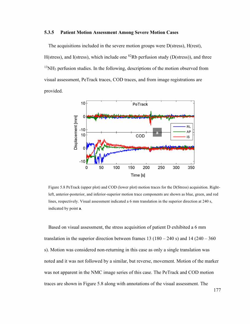
177

5.3.5 Patient Motion Assessment Among Severe Motion Cases

The acquisitions included in the severe motion groups were D(stress), H(rest),

H(stress), and I(stress), which include one 82Rb perfusion study (D(stress)), and three

13NH3 perfusion studies. In the following, descriptions of the motion observed from

visual assessment, PeTrack traces, COD traces, and from image registrations are

provided.

Figure 5.8 PeTrack (upper plot) and COD (lower plot) motion traces for the D(Stress) acquisition. Right-

left, anterior-posterior, and inferior-superior motion trace components are shown as blue, green, and red

lines, respectively. Visual assessment indicated a 6 mm translation in the superior direction at 240 s,

indicated by point a.

Based on visual assessment, the stress acquisition of patient D exhibited a 6 mm

translation in the superior direction between frames 13 (180 – 240 s) and 14 (240 – 360

s). Motion was considered non-returning in this case as only a single translation was

noted and it was not followed by a similar, but reverse, movement. Motion of the marker

was not apparent in the NMC image series of this case. The PeTrack and COD motion

traces are shown in Figure 5.8 along with annotations of the visual assessment. The

178

PeTrack motion trace indicated a rapid change in the marker position beginning around

210 s and lasting roughly 10 s, where the marker moved in the inferior direction and then

superiorly, coming to rest around 220 s at a position slightly inferior to its initial position.

The COD trace indicated a protracted shift from right to left, and anterior to posterior

starting with the acquisitions and ending around 175 s. Additionally, motion toward the

superior and then inferior directions was observed over the same span of time. Both

PT6D and CD6D approaches (image registration based) indicated frequent translation of

2 mm magnitude in all directions of motion between 50 s and 125 s as well as rotational

motion around 30 s.

Visual assessment of the rest acquisition of patient H exhibited protracted translations

beginning at frame 14 (240 – 360 s) and continued thereafter until the end of the

acquisition (1200 s). The accumulated motion consisted of translations in the superior

direction of roughly 7 mm, and smaller translation (~ 3 mm) in the left and posterior

directions. Superior and posterior translations of 10 mm and 3 mm, respectively, were

observed for the fiducial markers over the same span of time. Patient motion was non-

returning in this case. The PeTrack and COD motion traces are shown in Figure 5.9 along

with annotations of the visual assessment. The PeTrack motion trace indicated a

consistent superior and posterior drift from the beginning of the acquisition until the end

which spanned approximately 8 mm, and 5 mm, respectively. The COD traces indicated a

rapid rise near the beginning of the acquisition suggesting the COD position moved from

right to left, inferior to superior and anterior to posterior and then an asymptotic decay

toward the right, inferior, and anterior direction. Both PT6D and CD6D indicated similar

translation as for the D(Stress) acquisition and effectively no rotational motion.

179

The stress acquisition of patient H exhibited the largest extent and most complex

motion of any acquisitions included in this study. In the span of frames 13 (180 – 240 s)

to 15 (360 – 600 s) a lateral (to the right) translation of roughly 10 mm was evident.

Within this span, a counter-clockwise rotation in the transverse plane was also observed

Figure 5.9 PeTrack (upper plot) and COD (lower plot) motion traces for the H(Rest) acquisition. Right-

left, anterior-posterior, and inferior-superior motion trace components are shown as blue, green, and red

lines, respectively. Visual assessment indicated a protracted 7 mm translation in the superior direction

beginning between 240 and 360 s (indicated by point a) and continuing until the end of the acquisition.

between frames 13 and 14 (240 – 360 s). Frame 14 exhibited obvious motion blur.

Subsequently, clockwise rotations were observed in the transverse view between frames

15 and 17 (900 – 1200 s) which had an effect like lateral (to the left) and posterior

translations of roughly 3 mm and 5 mm, respectively. Motion was considered to be

returning for this case. Similar translations to those just described were observed for the

fiducial marker, although the translation to the right between frames 13 and 15 had a

greater extent; roughly 12 mm. The PeTrack and COD motion traces are shown in Figure

5.10 along with annotations of the visual assessment. The PeTrack motion trace appeared

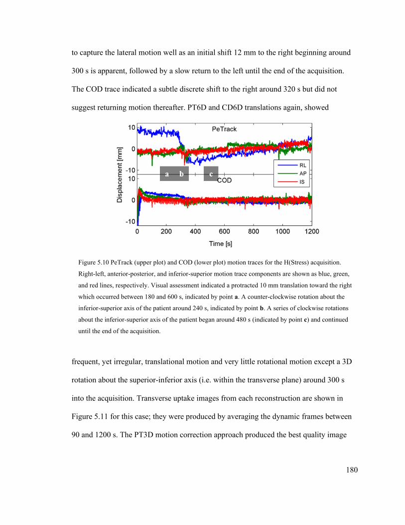
180

to capture the lateral motion well as an initial shift 12 mm to the right beginning around

300 s is apparent, followed by a slow return to the left until the end of the acquisition.

The COD trace indicated a subtle discrete shift to the right around 320 s but did not

suggest returning motion thereafter. PT6D and CD6D translations again, showed

Figure 5.10 PeTrack (upper plot) and COD (lower plot) motion traces for the H(Stress) acquisition.

Right-left, anterior-posterior, and inferior-superior motion trace components are shown as blue, green,

and red lines, respectively. Visual assessment indicated a protracted 10 mm translation toward the right

which occurred between 180 and 600 s, indicated by point a. A counter-clockwise rotation about the

inferior-superior axis of the patient around 240 s, indicated by point b. A series of clockwise rotations

about the inferior-superior axis of the patient began around 480 s (indicated by point c) and continued

until the end of the acquisition.

frequent, yet irregular, translational motion and very little rotational motion except a 3D

rotation about the superior-inferior axis (i.e. within the transverse plane) around 300 s

into the acquisition. Transverse uptake images from each reconstruction are shown in

Figure 5.11 for this case; they were produced by averaging the dynamic frames between

90 and 1200 s. The PT3D motion correction approach produced the best quality image

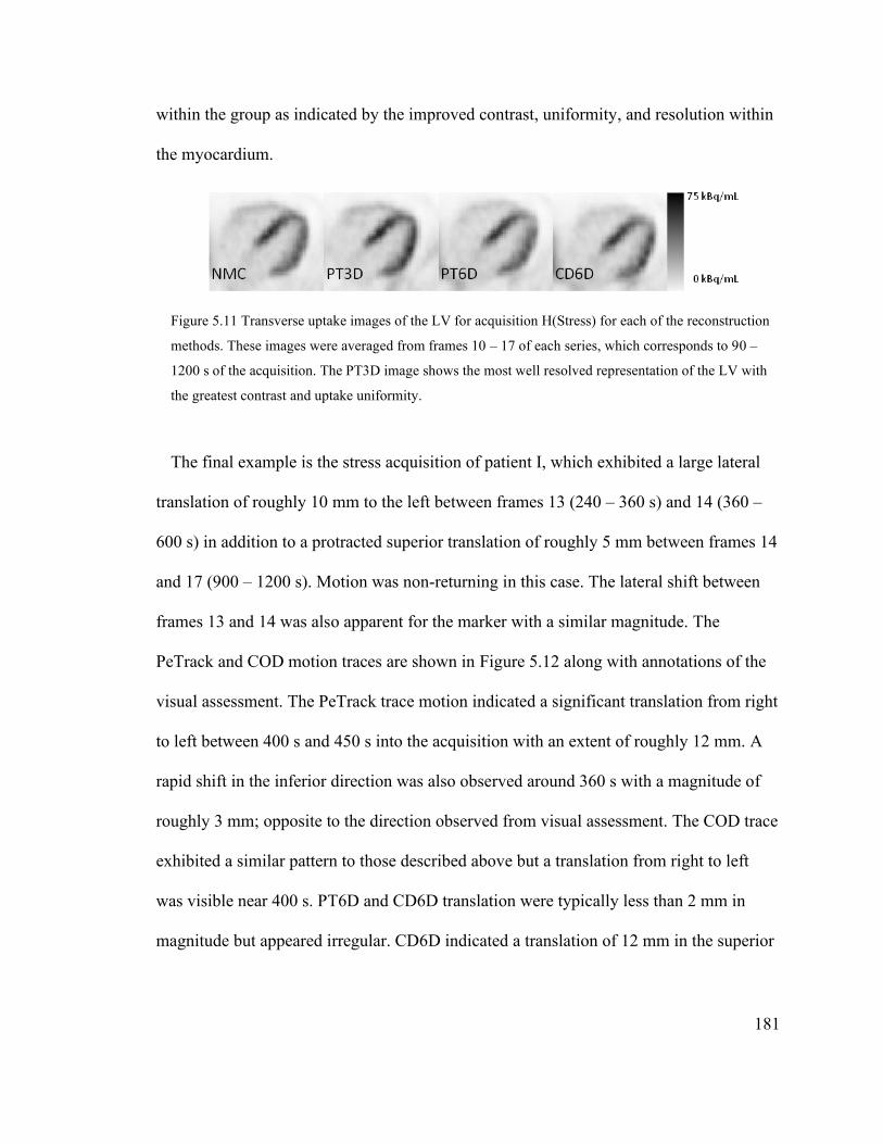
181

within the group as indicated by the improved contrast, uniformity, and resolution within

the myocardium.

Figure 5.11 Transverse uptake images of the LV for acquisition H(Stress) for each of the reconstruction

methods. These images were averaged from frames 10 – 17 of each series, which corresponds to 90 –

1200 s of the acquisition. The PT3D image shows the most well resolved representation of the LV with

the greatest contrast and uptake uniformity.

The final example is the stress acquisition of patient I, which exhibited a large lateral

translation of roughly 10 mm to the left between frames 13 (240 – 360 s) and 14 (360 –

600 s) in addition to a protracted superior translation of roughly 5 mm between frames 14

and 17 (900 – 1200 s). Motion was non-returning in this case. The lateral shift between

frames 13 and 14 was also apparent for the marker with a similar magnitude. The

PeTrack and COD motion traces are shown in Figure 5.12 along with annotations of the

visual assessment. The PeTrack trace motion indicated a significant translation from right

to left between 400 s and 450 s into the acquisition with an extent of roughly 12 mm. A

rapid shift in the inferior direction was also observed around 360 s with a magnitude of

roughly 3 mm; opposite to the direction observed from visual assessment. The COD trace

exhibited a similar pattern to those described above but a translation from right to left

was visible near 400 s. PT6D and CD6D translation were typically less than 2 mm in

magnitude but appeared irregular. CD6D indicated a translation of 12 mm in the superior

182

direction around 50 s. Effectively no rotational motion was indicated for either PT6D or

CD6D.

Figure 5.12 PeTrack (upper plot) and COD (lower plot) motion traces for the I(Stress) acquisition. Right-

left, anterior-posterior, and inferior-superior motion trace components are shown as blue, green, and red

lines, respectively. Visual assessment indicated a 10 mm translation toward the left which occurred

around 360 s, indicated by point a. A protracted superior translation of 5 mm was also observed starting

after 360 s and continuing until the end of the acquisition, indicated by point b.

5.3.6 Kinetic Modelling Results Among Severe Motion Cases

Absolute myocardial blood flow was compared for the severe motion cases before and

after each motion correction approach. A summary of the MBF measurements is shown

in Figure 5.13. In this plot the data are categorized by acquisition with data points for

each reconstruction method. The PT6D and CD6D motion correction methods generally

exhibited increased MBF variability across the myocardium compared to the

measurements from the NMC reconstructions. Otherwise, no obvious trends in these

measurements were apparent. The mean values of MBF, for instance, did not have

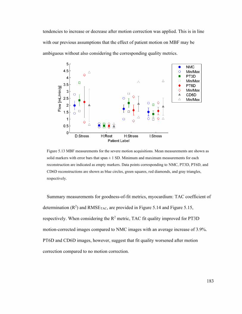
183

tendencies to increase or decrease after motion correction was applied. This is in line

with our previous assumptions that the effect of patient motion on MBF may be

ambiguous without also considering the corresponding quality metrics.

Figure 5.13 MBF measurements for the severe motion acquisitions. Mean measurements are shown as

solid markers with error bars that span ± 1 SD. Minimum and maximum measurements for each

reconstruction are indicated as empty markers. Data points corresponding to NMC, PT3D, PT6D, and

CD6D reconstructions are shown as blue circles, green squares, red diamonds, and gray triangles,

respectively.

Summary measurements for goodness-of-fit metrics, myocardium: TAC coefficient of

determination (R2) and RMSETAC, are provided in Figure 5.14 and Figure 5.15,

respectively. When considering the R2 metric, TAC fit quality improved for PT3D

motion-corrected images compared to NMC images with an average increase of 3.9%.

PT6D and CD6D images, however, suggest that fit quality worsened after motion

correction compared to no motion correction.

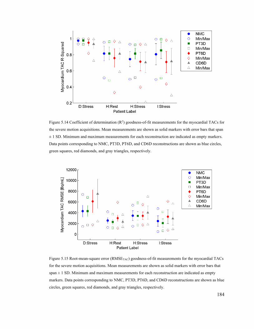
184

Figure 5.14 Coefficient of determination (R2) goodness-of-fit measurements for the myocardial TACs for

the severe motion acquisitions. Mean measurements are shown as solid markers with error bars that span

± 1 SD. Minimum and maximum measurements for each reconstruction are indicated as empty markers.

Data points corresponding to NMC, PT3D, PT6D, and CD6D reconstructions are shown as blue circles,

green squares, red diamonds, and gray triangles, respectively.

Figure 5.15 Root-mean-square error (RMSETAC) goodness-of-fit measurements for the myocardial TACs

for the severe motion acquisitions. Mean measurements are shown as solid markers with error bars that

span ± 1 SD. Minimum and maximum measurements for each reconstruction are indicated as empty

markers. Data points corresponding to NMC, PT3D, PT6D, and CD6D reconstructions are shown as blue

circles, green squares, red diamonds, and gray triangles, respectively.

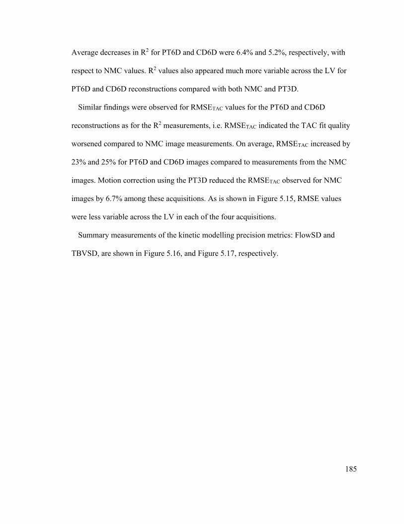
185

Average decreases in R2 for PT6D and CD6D were 6.4% and 5.2%, respectively, with

respect to NMC values. R2 values also appeared much more variable across the LV for

PT6D and CD6D reconstructions compared with both NMC and PT3D.

Similar findings were observed for RMSETAC values for the PT6D and CD6D

reconstructions as for the R2 measurements, i.e. RMSETAC indicated the TAC fit quality

worsened compared to NMC image measurements. On average, RMSETAC increased by

23% and 25% for PT6D and CD6D images compared to measurements from the NMC

images. Motion correction using the PT3D reduced the RMSETAC observed for NMC

images by 6.7% among these acquisitions. As is shown in Figure 5.15, RMSE values

were less variable across the LV in each of the four acquisitions.

Summary measurements of the kinetic modelling precision metrics: FlowSD and

TBVSD, are shown in Figure 5.16, and Figure 5.17, respectively.

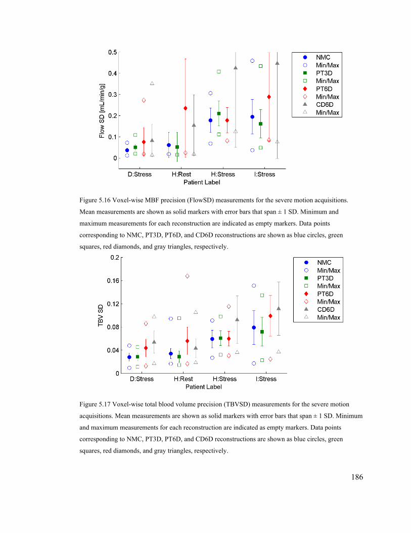
186

Figure 5.16 Voxel-wise MBF precision (FlowSD) measurements for the severe motion acquisitions.

Mean measurements are shown as solid markers with error bars that span ± 1 SD. Minimum and

maximum measurements for each reconstruction are indicated as empty markers. Data points

corresponding to NMC, PT3D, PT6D, and CD6D reconstructions are shown as blue circles, green

squares, red diamonds, and gray triangles, respectively.

Figure 5.17 Voxel-wise total blood volume precision (TBVSD) measurements for the severe motion

acquisitions. Mean measurements are shown as solid markers with error bars that span ± 1 SD. Minimum

and maximum measurements for each reconstruction are indicated as empty markers. Data points

corresponding to NMC, PT3D, PT6D, and CD6D reconstructions are shown as blue circles, green

squares, red diamonds, and gray triangles, respectively.

187

Among the four severe motion acquisitions, average FlowSD values increased by 5.2%,

110%, and 130% compared to values measured from NMC images, for PT3D, PT6D, and

CD6D motion correction reconstructions, respectively, As FlowSD values were expected

to increase with motion, this metric did not indicate a benefit from employing motion

correction. The precision of the total blood volume estimates showed a modest

improvement for the PT3D motion corrected images; TBVSD was reduced by -5.2% with

respect to values of the NMC images. TBVSD was increased for the PT6D and CD6D

reconstructions compared to the NMC images by 37% and 54%, respectively. Once more

this suggests that the PT6D and CD6D approaches to motion correction did not improve

MBF precision.

5.4 Discussion

Overall, the results suggested that motion tracking with either PeTrack or COD

methods is feasible but only the PT3D motion correction method seemed to be robust

enough for use during MBF estimation from dynamic cardiac PET perfusion studies.

Image registration did not demonstrate successful ability to compensate for the motion

that was observed among the severe motion cases. These results are largely preliminary,

however, as the size of the cohort was relatively small and, more importantly, the number

of the acquisitions which exhibited severe motion was very limited. It follows that a

rigorous statistical analysis of the measured data is not appropriate and conclusive

evidence regarding the use of any of these motion correction approaches was not

demonstrated within a general population of patients. Nevertheless, when treated as a

188

series of case studies, various valuable insights were gleaned that are discussed in the

following.

5.4.1 Motion Estimation with PeTrack

Generally, PeTrack produced patient-motion estimates that agreed with visual

assessment of the original NMC images. Among the severe motion cases detailed above,

the PT3D approach to motion corrections generally led to improvements in the various

quality metrics that were considered. The H(Stress) acquisition was the most compelling

example of the benefit of the PT3D motion correction approach. Polar maps of

myocardium TAC R2 values are shown for the NMC and PT3D reconstructions for the

H(Stress) acquisition in Figure 5.18. The NMC images exhibited returning motion

predominantly along the lateral direction. The R2 polar map from the NMC images shows

that TAC goodness-of-fit was reduced within the septal and lateral walls as would be

expected for severe lateral motion. Following PT3D motion correction, fit quality in these

regions was markedly improved which resulted in an increased MBF estimation for this

acquisition.

In one of the mild motion cases, acquisition C(Rest), marker motion indicated a non-

returning translation of roughly 5 mm in the inferior direction around 100 s into the

acquisition; this motion was confirmed at the marker by visual assessment. The marker

motion was discordant however with the motion of the LV and the PT3D motion

correction images led to a 10% increase in MBF, which was predominantly associated

with changes in the inferior wall at the apical level.

189

Figure 5.18 LV polar maps depicting coefficient of determination (R2) values for the myocardium TACs

for the NMC and PT3D images for the H(Stress) acquisition. Anatomic labels ‘A’, ‘S’, ‘L’, and ‘P’

correspond to the anterior, septal, lateral, and posterior regions of the LV, respectively. Motion

correction with PT3D approach improved R2 values in the septal and lateral regions of the LV in the

presence of severe lateral patient motion.

These two examples contrasted one another in the sense the marker motion may or may

not be an accurate surrogate for the body motion that occurred during the acquisition and

thus have varying degrees of success, or failure, to align dynamic frames prior to MBF

estimation via kinetic modelling. The use of PeTrack with a single marker is limited to

3D translation motion estimation. Future work should extend to the use of multiple

markers such that the assessment of various rotations can also be included. Based on the

visual assessment performed of the NMC images, rotations about the superior-inferior

axis of the patient would be of principal interest.

5.4.2 COD Motion Estimation

As was expected from the initial phantom studies, the COD motion traces were

dominated by the redistribution of the perfusion tracers within the body. A characteristic

pattern was apparent among all the COD motion traces for the patient cohort. The COD

trace of the B(Stress) acquisition is shown in Figure 5.19 to help describe the behaviour.

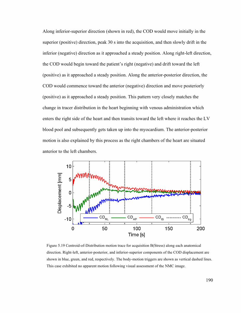
190

Along inferior-superior direction (shown in red), the COD would move initially in the

superior (positive) direction, peak 30 s into the acquisition, and then slowly drift in the

inferior (negative) direction as it approached a steady position. Along right-left direction,

the COD would begin toward the patient’s right (negative) and drift toward the left

(positive) as it approached a steady position. Along the anterior-posterior direction, the

COD would commence toward the anterior (negative) direction and move posteriorly

(positive) as it approached a steady position. This pattern very closely matches the

change in tracer distribution in the heart beginning with venous administration which

enters the right side of the heart and then transits toward the left where it reaches the LV

blood pool and subsequently gets taken up into the myocardium. The anterior-posterior

motion is also explained by this process as the right chambers of the heart are situated

anterior to the left chambers.

Figure 5.19 Centroid-of-Distribution motion trace for acquisition B(Stress) along each anatomical

direction. Right-left, anterior-posterior, and inferior-superior components of the COD displacement are

shown in blue, green, and red, respectively. The body-motion triggers are shown as vertical dashed lines.

This case exhibited no apparent motion following visual assessment of the NMC image.

191

While the COD trace was dominated by tracer dynamics, especially, prior to steady-

state uptake in the LV, detecting body motion was challenging. This is demonstrated in

Figure 5.19 by the large number of body motion triggers that were detected. In

comparison, the PeTrack motion trace for this acquisition demonstrates a very stable

position with displacements from the reference position < 1 mm for all directions of

motion. Moreover, no triggers were detected for this acquisition from the PeTrack motion

trace. PT6D and CD6D motion correction approaches both introduced inter-frame motion

that was not present in the NMC series, which had adverse effects on the kinetic

modelling outcomes for this acquisition like an artifactual increase in MBF, increased

MBF heterogeneity across the LV, and reduced TAC goodness-of-fit as indicated by

lower R2 values.

A periodic signal component is also visible within the COD trace shown (Figure 5.19)

for the B(Stress) acquisition which has a larger amplitude earlier in the acquisition before

the tracer has experienced much decay. The period appears to be on the order of 3

seconds which suggests that it is associated with respiratory motion. While respiratory,

and possibly, cardiac motion tracking was not a focus of this study, it appears that COD

motion tracking may be useful for these applications within cardiac perfusion PET

studies. While COD motion tracking has been applied to respiratory motion

compensation in previous studies118,189, it has not been demonstrated for cardiac perfusion

PET. This would be an interesting future research question.

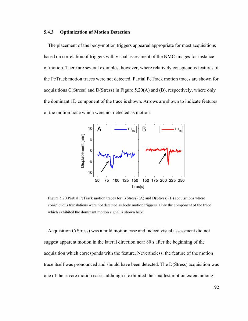
192

5.4.3 Optimization of Motion Detection

The placement of the body-motion triggers appeared appropriate for most acquisitions

based on correlation of triggers with visual assessment of the NMC images for instance

of motion. There are several examples, however, where relatively conspicuous features of

the PeTrack motion traces were not detected. Partial PeTrack motion traces are shown for

acquisitions C(Stress) and D(Stress) in Figure 5.20(A) and (B), respectively, where only

the dominant 1D component of the trace is shown. Arrows are shown to indicate features

of the motion trace which were not detected as motion.

Figure 5.20 Partial PeTrack motion traces for C(Stress) (A) and D(Stress) (B) acquisitions where

conspicuous translations were not detected as body motion triggers. Only the component of the trace

which exhibited the dominant motion signal is shown here.

Acquisition C(Stress) was a mild motion case and indeed visual assessment did not

suggest apparent motion in the lateral direction near 80 s after the beginning of the

acquisition which corresponds with the feature. Nevertheless, the feature of the motion

trace itself was pronounced and should have been detected. The D(Stress) acquisition was

one of the severe motion cases, although it exhibited the smallest motion extent among

193

that group. The missed feature appeared as a very short pulse in the motion trace but

corresponded to the beginning of a non-returning shift of the patient in the superior

direction as seen on the NMC image series. Marker motion was not apparent in NMC

image and, interestingly, the PeTrack motion trace suggested that the marker was

translated toward the inferior direction following a sharp pulse near 215 s.

The method by which body motion triggers were detected was developed with the use

of a relatively small subset of the acquisitions included in this study and the method is

unlikely to be optimized with respect to sensitivity and specificity for a general patient

population. The optimization process would involve adjusting the parameters of the

method related to smoothing of the traces as well as the size of the sliding window used

to compute the local normal vector orientation. As was indicated previously, other

methods were considered for the motion detection. The first approach was described in

Chapter 4, which involved the use of local displacement thresholds which, when

exceeded, resulted in a motion trigger. While this method worked very effectively for

PeTrack, it did not translate well for use with COD tracking. Another approach was based

on the two-sample Student’s t-test, where significant changes in the mean displacement

among adjacent windows led to a motion trigger. This method required careful tuning of

the significance level that corresponded to instances of suspected motion. This method

worked effectively for either PeTrack or COD (using different criteria), but not both. A

final method made use of a common signal-processing methods for peak detection; the

Laplacian of a Gaussian filter190 was applied to the traces in order detect peak in the

signals. Once again, however, the nature of the PeTrack and COD traces were too

194

different to permit similar sets of body-motion triggers among the test cases used for

development.

Sun et al.180 examined the use of data-driven motion tracking method which was

technically very similar to the COD method. They developed a novel approach to detect

instance of body motion which was based on a single scalar metric which was computed

as the sum of the eigenvalues of the covariance matrix and the 3D motion trace within a

sliding window. Their results suggested that body motions of 12 mm or rotations of 20º

could be detected with good accuracy. The PET studies in their work used 18F-based

tracers with delayed acquisitions and so they did not evaluate their work under the

conditions presented here. The authors caution that their method may not translate well to

perfusion studies such as discussed herein.

Others have circumvented issues associated with limited motion detection

sensitivity/specificity by incorporating high temporal resolution motion estimation

directly into the reconstruction process. Such an approach was recently investigated by

Armstrong et al.191 where they performed 3D image registrations on low resolution back-

projected images of 1-second durations to estimate motion during static 82Rb cardiac PET

MPI studies. In their preliminary work they incorporated the axial component of motion

only directly into the reconstruction process ignoring lateral or anterior-posterior motion.

Such an approach is likely to be more appropriate to compensate specifically for

respiratory motion. In dynamic cardiac PET studies lateral motion of the LV, specifically

towards the left lung, has been shown to lead to significant changes in MBF estimation.82

A similar approach which used PeTrack was recently reported by Chamberland, Xu,

deKemp92 with promising results, but in their case individual LORs were re-positioned

195

prior to reconstruction. To apply such an approach directly to the motion tracking data

may not always be effective, however, if the PeTrack marker motion does not accurately

represent motion of the heart. Similar arguments may apply to COD tracking.

As a final comment regarding motion detection while using COD tracking, the fact that

a relatively consistent COD motion trace pattern was observed among the cohort suggests

that a model motion trace could be estimated from a large cohort where no patient motion

occurred. The model could potentially be fit to future COD motion traces to assess

whether any significant deviation from the model occurred. These deviations, if not

associated with the pattern of normal tracer dynamics in the body, could be interpreted as

instances of motion.

5.4.4 Motion Estimation Using Image Registration

Despite the initial efforts to set up the image registration framework in a robust and

accurate fashion using the phantom acquisitions, the PT6D and CD6D images generally

produced varying degrees of motion artifacts in the dynamic series. Visually, this often

appeared as jittering of adjacent dynamic frames. In other cases, it was clear that changes

in the tracer distribution in in the earlier frames, as seen from the NMC images, were

interpreted as spatial misalignment during image registration and they were over-

corrected. These limitations of the image-registration scheme for estimation of patient

motion significantly limit the assessment of the COD tracking approach as no other

motion estimation approach was considered for it.

The most extreme example of failure of the image registration to estimate motion was

observed for acquisition B(Rest) for both PT6D and CD6D images. The largest inter-

196

frame translations and rotations were ~40 mm, and ~20º, respectively, for both PT6D and

CD6D images. In contrast, this acquisition was considered as a mild motion case using

visual assessment and the largest inter-frame translation (based on changes in mean

PeTrack positions between adjacent frames) was 2 mm. The registration failure in this

case may be associated with low count motion frame images within the registration

sequence as well as disparate tracer distributions among early frames. The sequential

registration method is inherently sensitive to the problem of poor registrations within the

sequence. The novel approach to automated alignment of dynamic cardiac perfusion

frames described by Lee and colleagues81 which uses distinct reference frames in the

early blood pool and late uptake portions of the dynamic series could be implemented

here to overcome this issue.

It could be argued that extending the motion model to include rotations disadvantaged

the PT6D and CD6D compared to PT3D. Complex models with a larger number of free

parameters are generally less robust to noise and small data sizes. This pitfall was not

obvious at the outset of this work, as the motion model with six degrees of freedom is

still a rigid model and each image volume contains more than 7.7×105 voxels which

contribute to the registration process. Moreover, others have reported successful

registration results using more complex motion models119, although not in the application

of dynamic cardiac PET perfusion studies.

The performance of the image registration technique described in this work could be

enhanced in future work by considering the following amendments. First, the motion

model could be reduced to include only 3D translations. Second, the initial non-

attenuation corrected dynamic reconstruction used for image registration could

197

completely ignore the clinical dynamic sequence and reconstruct only frames that are

identified in the motion detection step. In doing so, many fewer frames would be

reconstructed (enhancing the counts in each) and the estimated motion model would be

applied to all dynamic frames that fall within the corresponding motion frame. Third, the

image registration could be regularized by applying additional smoothing to the non-

attenuation corrected images used to estimate motion. Later, when applying the

registration transformations for motion correction, the original (un-smoothed) images

could still be used. Fourth, the duration of the smallest permissible motion frames could

be adjusted throughout the acquisition based on the decay of the tracer. In this way, at

later time points in the acquisition the shortest frame duration would be increased to have

similar lower limits on the counts compared to earlier time points before the tracer has

appreciably decayed. Lastly, the sensitivity of the motion detection method could be

reduced such that fewer frames are reconstructed, and each would have a higher count

density; although this would impair the overall effectiveness of the motion correction

method.

5.4.5 Classification of Cases Which Could Benefit from Motion Correction

As was observed in this cohort, the majority of acquisitions corresponded to no or mild

motion and did not benefit from the application of motion correction. More importantly,

the quality of MBF estimation for some cases was negatively affected following motion

correction (particularly for the PT6D and CD6D approaches). This finding leads to the

question: how does one choose which scans would benefit from motion correction? In

some case motion may be so severe that this decision would be obvious. The cohort in

198

this study, however, largely does not meet that criterion. Nevertheless, patient motion

correction has regularly been identified as a contributing factor to the overall repeatability

of MBF estimation77,81,85,184 and so a robust and automated method with which cases

could be classified as those which would benefit from motion correction could be very

clinically useful, especially for fringe cases where the motion effects are not obvious.

Carrying on with this notion, a metric (or set of metrics) must be determined which can

flag acquisitions where motion either possibly or probably affected the accuracy of the

MBF estimation. The quality metrics examined in this work have been suggested by

others as being relevant indicators of the presence patient of motion, but they may not all

agree with each other on an individual basis. In Table 5.1 it was shown that the

coefficient of determination (R2) and root-mean-square error (RMSETAC) of the

myocardial TAC fits did not show the same trend between the mild and severe motion

cases. Moreover, the changes observed in all of the quality metrics between the mild and

severe motion groups may be confounded by the choice of perfusion tracer, the duration

of the acquisition, and/or the number of dynamic frames used as part of the kinetic

model. For example, 3 out of the 4 severe motion cases corresponded to 13NH3 perfusion

studies which are 20 minutes in duration and use 17 dynamic frames. Conversely, 11 out

of the 13 mild motion cases were 82Rb perfusion studies only 6 minutes of which (14

dynamic frames) were used for kinetic modelling.

Relying on visual assessment of motion within the dynamic images may not always be

reliable. In this work, visual motion assessment in the early frames prior to myocardial

uptake was very challenging largely due to the rapid changes in tracer distribution as well

as its diffuse appearance throughout the body. It follows that visual detection of motion

199

was limited to the later uptake frames and thus corresponds to a relatively small number

of frames used in kinetic modelling. This issue was also reported in the work of Lee et

al.,81 in regard to automated alignment of dynamic frames of 82Rb cardiac PET perfusion

studies.

It may be that within a general population of patients that a multivariate analysis of

MBF quality metrics and automated motion estimation approaches would provide more

satisfactory and robust classification. Such a problem seems to lend itself to machine

learning solutions which can combine different sources of data to make classification

predictions. No other published research on this specific topic was found at the time this

work was written.

5.5 Conclusions

Motion correction in cardiac PET perfusion studies based on the 3D translational

motion information produced by PeTrack appeared feasible and more robust than image-

registration approaches. Additional research on this application is warranted with a larger

patient population and with more cases of severe motion to further develop the proposed

motion correction algorithm. While the COD method demonstrated potential benefits

over PeTrack like its independence of any additional equipment and its fast computation

time, its use in cardiac PET perfusion studies is limited as the absolute displacement

indicated by COD does not accurately represent the observed motion of the heart and

necessitates the use of image-registration techniques to estimate motion. Additionally, the

COD trace is inherently linked to the tracer dynamics in the body and detecting instances

of patient motion prior to myocardial uptake remains challenging. Future work regarding

200

the classification of clinical cases that would benefit from motion correction remains as

an interesting research question.

201

Chapter 6 Conclusions and Future Work

6.1 Summary of Findings

The motion information derived from the PeTrack ADROI algorithm was used to

implement a data-driven alternative to respiratory motion tracking and gating, as well as a

body-motion detection and compensation tool for cardiac PET perfusion imaging studies.

This thesis described the most comprehensive application of the PeTrack algorithm in a

clinical setting.

When used for respiratory gating in a general population of patients for which cardiac

perfusion PET was indicated, it was shown that respiratory gating with PeTrack is

feasible and its performance was comparable to one of the most commonly used

hardware-based respiratory motion tracking systems. Respiratory signal quality was

generally better for the optical tracking system but its efficacy for respiratory gating was

hindered by its technical limitations. The gating quality of the optical system was

improved using the retrospective respiratory trigger detection technique that was

implemented for PeTrack in this thesis. This work also exposed short comings of the

PeTrack algorithm that will need to be addressed before this tool could be shown to be

unequivocally beneficial in the presence of significant respiratory motion.

Whole body motion correction was explored in the context of static and dynamic

cardiac PET perfusion studies. For this purpose, a novel framework for including the

PeTrack motion information was developed and incorporated into the research

reconstruction software. A series of phantom acquisitions with relatively extreme motion

showed significant benefit from motion correction using the PeTrack approach with

202

respect to recovery of image quality metrics like myocardial contrast-to-noise, and signal-

to-noise ratios as well as the LV wall thickness (an indicator of the effective spatial

resolution in the presence of motion). The same motion correction strategy was also

employed for a small cohort of 13N-ammonia perfusion studies for which the benefits of

PeTrack-based motion correction were not as obvious. While image quality metrics

generally showed improvement after motion correction, especially reduced LV wall

thickness, no apparent effect could be demonstrated on the relative perfusion

measurements among this group. This work suggested that patient motion using this

approach was feasible and generally led to improve image quality. The clinical

significance of the approach, however, may not be realized without the presence of non-

returning patient motion in excess of 10 mm.

Finally, the body motion correction framework was extended to dynamic studies and

absolute blood flow quantification. The data-driven centroid-of-distribution motion

tracking method which was reported to be successful for dynamic PET studies was also

implemented for comparison with the PeTrack approach. This work showed that tracking

the motion of a fiducial marker as opposed to the centroid-of-distribution may be more

robust when applied to cardiac PET perfusion imaging when motion tracking is required

in the early frames before the tracer distribution has reached equilibrium in the body.

Inferring patient motion from the purely data-driven motion signal was challenging as the

signal was dominated by tracer dynamics. Additionally, image registration techniques did

not appear to be sufficiently robust to adequately estimate patient motion from the

dynamic series of motion frames. Motion correction based on 3D motion estimation

directly from the PeTrack motion trace was more reliable in this context than the

203

approaches which used image registration. Various quality metrics related to blood flow

quantification that are generally regarded to be correlated with motion severity were

considered. These data suggest that motion correction was not beneficial unless patient

motion magnitude exceeded 10 mm. In some cases, kinetic modelling quality metrics

suggested that motion correction had adverse effects, especially when image registration

was employed for motion estimation. Motion correction was thus not indicated for the

majority of acquisitions in the cohort. It follows that a decision algorithm based on a

combination of motion estimates and kinetic modelling quality metrics may be necessary

to select cases that are most likely to benefit from motion correction.

6.2 Final Thoughts and Suggestions for Future Work

This thesis indicated that additional work is required to enhance the motion tracking

signal as well as the robustness of the algorithm in the presence of high count rates

associated with high tracer activity concentrations in the patient. Under these conditions,

the noise in the PeTrack signal appeared to limit the accuracy of detecting respiratory

triggers when the external motion amplitudes were very small. In spite of the measures

implemented in ADROI to adapt the PeTrack algorithm for use in PET, marker tracking

failed in several cases when marker activity was very low in comparison to the scanner

count rates, i.e. less than 0.01%. To improve performance the most obvious solution is to

increase the marker activity. This solution was attempted with markers that had an

activity roughly three times that used for the work presented here, but their use was

suspended after observing deleterious effects on the scatter estimation of the GE

Discovery 690 scanner at UOHI. The activity of the marker was identified by the scanner

204

as existing outside the body and led to over-estimation of scatter and under-estimation of

the tracer activity within the body. It follows that a careful examination of the limits of

the marker activity and/or preparation of the attenuating material that surrounds the

marker to mimic extension of the body contour is needed to permit increasing the marker

activity.

Another important consideration is that the GE Discovery 690 PET/CT scanner is no

longer a state-of -the-art system. Digital PET/CT systems are now available, some with

an extended axial FOV, which exhibit much higher sensitivity, count-rate performance,

and improved TOF resolution. To date, motion tracking with PeTrack has not been

evaluated on one of these devices. It stands to reason that the hardware improvements

would be beneficial for PeTrack signal quality as well, as the systems are likely to have

improved sensitivity and specificity for detecting LORs coming from the marker which

are then used for tracking. Additionally, PeTrack may be of particular interest for

extended axial FOV scanners, like those engineered by the EXPLORER

consortium192,193, as optical motion tracking systems may be of limited use as the cameras

may not be able to monitor the patient effectively from outside the long bore.

To date, tracking multiple fiducial markers has only been attempted for phantom

acquisitions and has yet to be employed for clinical acquisitions. Tracking multiple

markers would permit the estimation of rotations as well as translations. To perform such

a task in the clinical environment would necessitate either a dedicated prospective study

or a modification to current clinical protocol at our clinic which already makes use of

single fiducial marker. Neither of these were seriously considered in the work presented

here. There are also several limitations associated with the use of multiple markers that

205

should be considered. PeTrack processing time would be expected to increase with the

number of markers used as only a single marker can be tracked in one instance of the

algorithm. Perhaps parallel computing technique could be explored to overcome this

obstacle. Additionally, a carefully designed system would likely be needed to fix the

markers in place on the patient. Use of a support like this is not favourable, however, as it

requires additional patient preparation and may not be tolerated well by all patients.

For future work for either evaluation or further development of PeTrack, special care

should be taken in accruing larger clinical data sets where patient motion (respiratory or

whole-body) is suspected to be significant. The work presented here included clinical

cohorts that were randomly selected from a general population. They did not encompass

enough cases with severe patient motion for which the benefits of respiratory gating

and/or motion compensation could be demonstrated with confidence. For the present

work, the possibility of including more studies with significant patient motion was

limited for several reasons. First, there was a limitation of the software of the PET system

to access list-mode data. In particular, the large data files are compressed using a

proprietary technique shortly after acquisition. The decompression software failed to

fully decompress large list-mode files that were acquired as part of a trial for a novel 18F-

based innervation tracer taking place at UOHI. These acquisitions are roughly 40 minutes

in duration and good candidates for significant patient motion. It was learned, however,

that the list-mode files which are required for PeTrack could not be decompressed for

use. Unfortunately, time did not permit working with the vendor to overcome this issue

and it was decided to make use of the 20-minute 13N-ammonia perfusion studies instead.

At UOHI, 13N-ammonia studies are almost exclusively acquired on the older GE

206

Discovery 600 PET/CT system which does not have TOF capability – an important

aspect of the ADROI extension of PeTrack. One acquisition was included from this

scanner for the work in Chapter 4, and 13N-ammonia acquisitions were few for the GE

Discovery 690 PET/CT system.

The work presented in this thesis supports the clinical usefulness of the PeTrack

ADROI algorithm for motion detection, estimation, and compensation in the context of

cardiac perfusion PET studies. This method simplifies patient preparation compared to

alternative hardware tracking systems and does not require technical integration with the

PET system. Furthermore, PeTrack was used in several cases to provide patient motion

information when hardware tracking systems failed during clinical use. PeTrack is easily

implemented in a high throughput clinical setting and can provide patient motion

information which characterizes both respiratory and body movements. To date, PeTrack

ADROI has only been implemented for GE Discovery series PET/CT scanners but it

could be adapted to other systems assuming that access to scanner geometry and

specifications can be attained. Lastly, the high temporal resolution motion vectors

provided by PeTrack could be readily incorporated into modern motion-compensated

image reconstruction algorithms. Further development of PeTrack holds promise for a

robust and easy-to-use motion compensation tool that can track multiple forms of patient

motion.

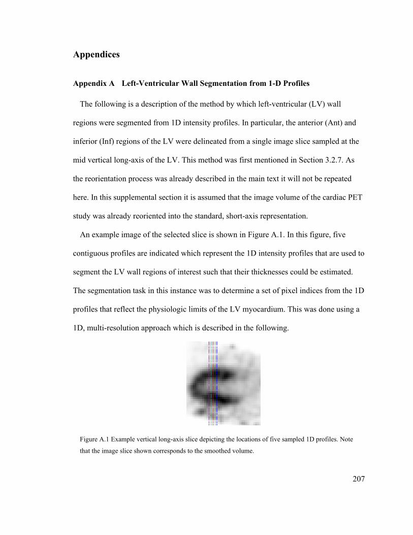
207

Appendices

Appendix A Left-Ventricular Wall Segmentation from 1-D Profiles

The following is a description of the method by which left-ventricular (LV) wall

regions were segmented from 1D intensity profiles. In particular, the anterior (Ant) and

inferior (Inf) regions of the LV were delineated from a single image slice sampled at the

mid vertical long-axis of the LV. This method was first mentioned in Section 3.2.7. As

the reorientation process was already described in the main text it will not be repeated

here. In this supplemental section it is assumed that the image volume of the cardiac PET

study was already reoriented into the standard, short-axis representation.

An example image of the selected slice is shown in Figure A.1. In this figure, five

contiguous profiles are indicated which represent the 1D intensity profiles that are used to

segment the LV wall regions of interest such that their thicknesses could be estimated.

The segmentation task in this instance was to determine a set of pixel indices from the 1D

profiles that reflect the physiologic limits of the LV myocardium. This was done using a

1D, multi-resolution approach which is described in the following.

Figure A.1 Example vertical long-axis slice depicting the locations of five sampled 1D profiles. Note

that the image slice shown corresponds to the smoothed volume.

208

The original image volume did not undergo any post-reconstruction smoothing. It thus

contained the highest spatial resolution representation of the image. It is referred to here

as the ‘raw’ volume. It was from this raw volume that the Ant and Inf wall region

thicknesses were determined. The noise level in the raw volume makes the task of

segmentation very challenging so it follows that a duplicate of the raw volume was

produced and then smoothed to initialize estimates of the relevant regions of interest

within the profiles. The smoothing kernel was a 3D Gaussian volume with a FWHM of

7.5 mm with a size of 5 × 5 × 5 voxels. Figure A.2 shows the 1D intensity profiles

extracted from the raw volume of the case shown in Figure A.1 and it is apparent that

identification of the Ant and Inf wall limits is not obvious. An assumption was made in

the development of this approach that over the short-axis span of the five profiles a single

set of limits could be generated that would accurately represent the limits of all of the five

profiles. Following this assumption, the five 1D profiles from each of the raw and smooth

volumes were averaged along the short-axis dimension to include the information from

all five profiles to aid the estimation of a single set of limits for each wall region. The

resulting mean profiles are referred to as the ‘avgRaw’ and ‘smooth’ profiles.

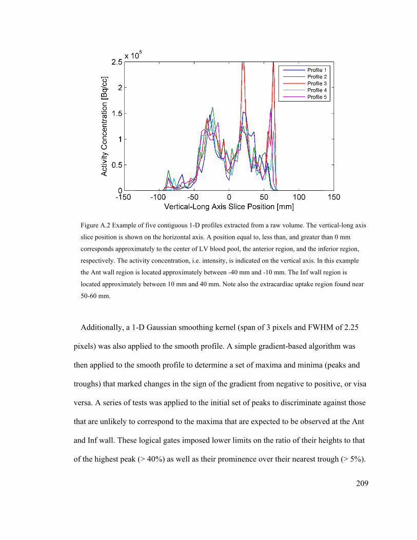
209

Figure A.2 Example of five contiguous 1-D profiles extracted from a raw volume. The vertical-long axis

slice position is shown on the horizontal axis. A position equal to, less than, and greater than 0 mm

corresponds approximately to the center of LV blood pool, the anterior region, and the inferior region,

respectively. The activity concentration, i.e. intensity, is indicated on the vertical axis. In this example

the Ant wall region is located approximately between -40 mm and -10 mm. The Inf wall region is

located approximately between 10 mm and 40 mm. Note also the extracardiac uptake region found near

50-60 mm.

Additionally, a 1-D Gaussian smoothing kernel (span of 3 pixels and FWHM of 2.25

pixels) was also applied to the smooth profile. A simple gradient-based algorithm was

then applied to the smooth profile to determine a set of maxima and minima (peaks and

troughs) that marked changes in the sign of the gradient from negative to positive, or visa

versa. A series of tests was applied to the initial set of peaks to discriminate against those

that are unlikely to correspond to the maxima that are expected to be observed at the Ant

and Inf wall. These logical gates imposed lower limits on the ratio of their heights to that

of the highest peak (> 40%) as well as their prominence over their nearest trough (> 5%).

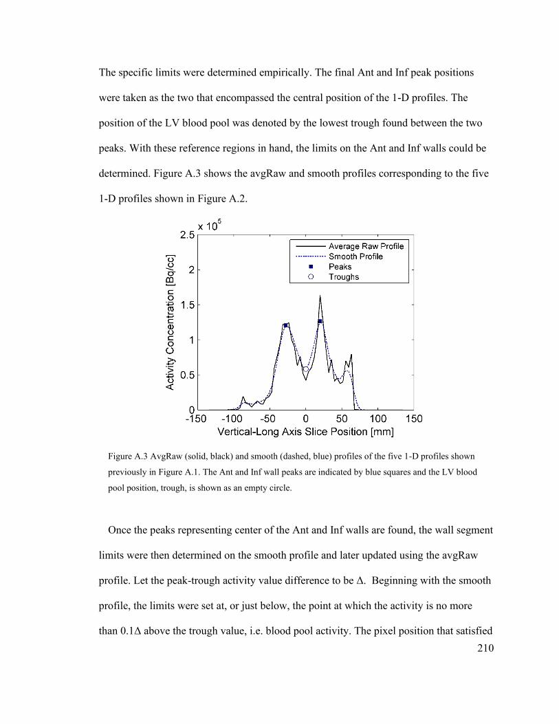
210

The specific limits were determined empirically. The final Ant and Inf peak positions

were taken as the two that encompassed the central position of the 1-D profiles. The

position of the LV blood pool was denoted by the lowest trough found between the two

peaks. With these reference regions in hand, the limits on the Ant and Inf walls could be

determined. Figure A.3 shows the avgRaw and smooth profiles corresponding to the five

1-D profiles shown in Figure A.2.

Figure A.3 AvgRaw (solid, black) and smooth (dashed, blue) profiles of the five 1-D profiles shown

previously in Figure A.1. The Ant and Inf wall peaks are indicated by blue squares and the LV blood

pool position, trough, is shown as an empty circle.

Once the peaks representing center of the Ant and Inf walls are found, the wall segment

limits were then determined on the smooth profile and later updated using the avgRaw

profile. Let the peak-trough activity value difference to be Δ. Beginning with the smooth

profile, the limits were set at, or just below, the point at which the activity is no more

than 0.1Δ above the trough value, i.e. blood pool activity. The pixel position that satisfied

211

this criterion, on both sides of the peak, was marked. Then using the avgRaw profile, a

search was performed for a point lower than the LV blood pool activity of the smooth

profile where an inflection occurred. The search space was limited to the region between

the smooth profile peak and the initial limit, i.e. the updated limit could not be further

separated from the peak than the initial limit. This process was applied in the following

order: outer Ant wall, inner Ant wall, inner Inf wall, and outer Inf wall. Its aim was to

constrain the domain of each wall region to myocardium and exclude the blood pool and

extracardiac regions. The final segmented wall regions are indicated in Figure A.4, which

is a duplicate of Figure A.3 except that the limits of the Ant and Inf walls are denoted and

the segmented Ant and Inf regions are shown in red and green, respectively.

Figure A.4 Replication of the avgRaw and smooth profiles shown in Figure A.3 but with the addition of

demarcations of the Ant and Inf wall limits (upward and downwards triangles, respectively) and

segmented regions (red and green lines, respectively).

212

It is important to note that this process was executed in a completely automated fashion

such that user bias did not affect the thickness measurements. Lastly, the segmentation

results were visually inspected for all images included in this study to evaluate their

success. In doing so, no cases were found that violated the assumption made previously

that a single set of limits would accurately represent the five unique short-axis positions.

213

Appendix B Elastix Image Registration Input Parameters

The following text is a duplication in the input parameters passed to the Elastix image

registration software package. This information was first cited in Section 5.2.3.

(FixedInternalImagePixelType "float")

(FixedImageDimension 3)

(MovingInternalImagePixelType "float")

(MovingImageDimension 3)

(Registration "MultiResolutionRegistration")

(FixedImagePyramid "FixedSmoothingImagePyramid")

(MovingImagePyramid "MovingSmoothingImagePyramid")

(Interpolator "BSplineInterpolator")

(Metric "AdvancedMattesMutualInformation")

(Optimizer "AdaptiveStochasticGradientDescent")

(ResampleInterpolator "FinalBSplineInterpolator")

(Resampler "DefaultResampler")

(Transform "EulerTransform")

(NumberOfResolutions 3)

(ImagePyramidSchedule 8 8 8 4 4 4 1 1 1)

(AutomaticTransformInitialization "true")

(AutomaticScalesEstimation "true")

(HowToCombineTransforms "Compose")

(ComputeZYX "true")

(MaximumNumberOfIterations 500)

(NumberOfHistogramBins 16)

(FixedLimitRangeRatio 0.001 0.01 0.01)

214

(MovingLimitRangeRatio 0.001 0.01 0.01)

(FixedKernelBSplineOrder 1)

(MovingKernelBSplineOrder 3)

(WriteTransformParametersEachIteration "false")

(WriteTransformParametersEachResolution "false")

(WriteResultImage "true")

(CompressResultImage "false")

(ResultImageFormat "mhd")

(ResultImagePixelType "float")

(ShowExactMetricValue "false")

(ErodeMask "true")

(UseDifferentiableOverlap "false")

(ImageSampler "Random")

(NumberOfSpatialSamples 2000)

(NewSamplesEveryIteration "true")

(BSplineInterpolationOrder 1)

(FinalBSplineInterpolationOrder 3)

(DefaultPixelValue 0)

215

References

1. Röntgen W. Sitzungsberichte Würzburger Physik-medic. Gesellschaft.

1895;137:132-141. https://web.lemoyne.edu/~giunta/ROENTGEN.HTML.

2. Taylor JR, Zafiratos CD, Dubson MA. Modern Physics For Scientists and

Engineers, 2nd Edition. Upper Saddle River, NJ: Pearson Prentice Hall; 2003.

3. Dalton J. On the Absorption of Gases by Water and other Liquids. In: Memoirs of

the Literary and Philosophical Society of Manchester. 2nd ed. London: R.

Bickerstaff, Strand; 1805:271-287.

4. Thomson JJ. XL. Cathode Rays . London, Edinburgh, Dublin Philos Mag J Sci.

1897;44(269):293-316. doi:10.1080/14786449708621070

5. Rutherford E. LXXIX. The scattering of α and β particles by matter and the

structure of the atom. London, Edinburgh, Dublin Philos Mag J Sci.

1911;21(125):669-688. doi:10.1080/14786440508637080

6. Rutherford E. LIV. Collision of α particles with light atoms . IV. An anomalous

effect in nitrogen . London, Edinburgh, Dublin Philos Mag J Sci.

1919;37(222):581-587. doi:10.1080/14786440608635919

7. Chadwick J. Possible Existence of a Neutron. Nature. 1932;129(3252):312-312.

doi:10.1038/129312a0

8. Becquerel H. Sur les radiations invisibles émises par les corps phosphorescents.

Comptes-rendus l’Académie des Sci séance du 1er mars 1896. 1896:501-502.

9. Sklodowska Curie M. Rays Emitted by Compounds of Uranium and of Thorium.

Comptes Rendus Hebd des Séance l’Académie des Sci Séance 12 April 1898.

216

1898;126:1101-1103.

10. Levin C. Basic Physics of Radionuclide Imaging. In: Wernick MN, Aarsvold

JNBT-ET, eds. Emission Tomography. San Diego: Academic Press; 2004:53-88.

doi:https://doi.org/10.1016/B978-012744482-6.50007-7

11. Krane KS. Introductory Nuclear Physics, 3rd Edition. Hoboken, NJ: John Wiley &

Sons, Ltd; 1987.

12. IAEA. Nuclear Medicine Physics. Vienna: International Atomic Energy Agency;

2015. https://www.iaea.org/publications/10368/nuclear-medicine-physics.

13. Knoll GF. Radiation Detection and Measurement. 3rd ed. New York: John Wiley

& Sons, Ltd; 2000.

14. Bé M-M, Chisté V, Dulieu C, et al. Table of Radionuclides. Vol 8. Pavillon de

Breteuil, F-92310 Sèvres, France: Bureau International des Poids et Mesures;

2016.

http://www.bipm.org/utils/common/pdf/monographieRI/Monographie_BIPM-

5_Tables_Vol8.pdf.

15. Rutherford Ernest. Radio-Activity. (Neville FH, Whetham FA, eds.). Cambridge,

UK: Cambridge: At the University Press; 1904.

https://www.biodiversitylibrary.org/item/127262.

16. Bateman, H. The solution of a system of differential equations occurring in the

theory of radio-active transformations. Proc Cambridge Phil Soc, 1908.

1908;15:423-427. http://ci.nii.ac.jp/naid/10020715519/en/. Accessed March 6,

2020.

17. IAEA. Diagnostic Radiology Physics. Vienna: International Atomic Energy

217

Agency; 2014. https://www.iaea.org/publications/8841/diagnostic-radiology-

physics.

18. Bethe H. Zur Theorie des Durchgangs schneller Korpuskularstrahlen durch

Materie. Ann Phys. 1930;397(3):325-400. doi:10.1002/andp.19303970303

19. Levin CS, Hoffman EJ. Calculation of positron range and its effect on the

fundamental limit of positron emission tomography system spatial resolution. Phys

Med Biol. 1999;44(3):781-799. doi:10.1088/0031-9155/44/3/019

20. Iwata K, Greaves RG, Surko CM. γ-ray spectra from positron annihilation on

atoms and molecules. Phys Rev A - At Mol Opt Phys. 1997;55(5):3586-3604.

doi:10.1103/PhysRevA.55.3586

21. Wernick MN, Aarsvold JN. Introduction to Emission Tomography. In: Wernick

MN, Aarsvold JNBT-ET, eds. Emission Tomography. 1st ed. San Diego:

Academic Press; 2004:11-23. doi:https://doi.org/10.1016/B978-012744482-

6.50005-3

22. Bailey DL, Karp JS, Surti S. Physics and Instrumentation in PET. In: Positron

Emission Tomography. London: Springer-Verlag; 2005:13-39. doi:10.1007/1-

84628-007-9_2

23. Wilkinson F. Scintillators. In: Wernick MN, Aarsvold JNBT-ET, eds. Emission

Tomography. San Diego: Academic Press; 2004:229-254.

doi:https://doi.org/10.1016/B978-012744482-6.50016-8

24. Pichler BJ, Ziegler SI. Photodetectors. In: Wernick MN, Aarsvold JNBT-ET, eds.

Emission Tomography. San Diego: Academic Press; 2004:255-267.

doi:https://doi.org/10.1016/B978-012744482-6.50017-X

218

25. Ghassemi A, Kobayashi K, Sato K. A Technical Guide to Silicon Photomultipliers

(MPPC). Hamamatsu City, Japan; 2018.

https://hub.hamamatsu.com/us/en/technical-note/sipm-mppc-technical-

note/index.html.

26. Zhang J, Maniawski P, Knopp M V. Performance evaluation of the next generation

solid-state digital photon counting PET/CT system. EJNMMI Res. 2018;8(1):97.

doi:10.1186/s13550-018-0448-7

27. Bettinardi V, Presotto L, Rapisarda E, Picchio M, Gianolli L, Gilardi MC. Physical

Performance of the new hybrid PET/CT Discovery-690. Med Phys.

2011;38(10):5394-5411. doi:10.1118/1.3635220

28. Kinahan PE, Defrise M, Clackdoyle R. Analytic Image Reconstruction Methods.

In: Wernick MN, Aarsvold JNBT-ET, eds. Emission Tomography. San Diego:

Academic Press; 2004:421-442. doi:https://doi.org/10.1016/B978-012744482-

6.50023-5

29. Bailey DL. Data Acquisition and Performance Characterization in PET. In:

Positron Emission Tomography. London: Springer-Verlag; 2006:41-62.

doi:10.1007/1-84628-007-9_3

30. Ishii K, Orihara H, Matsuzawa T, Binkley DM, Nutt R. High resolution time-of-

flight positron emission tomograph. Rev Sci Instrum. 1990;61(12):3755-3762.

doi:10.1063/1.1141549

31. Lewellyn T, Karp J. PET Systems. In: Wernick MN, Aarsvold JNBT-ET, eds.

Emission Tomography. San Diego: Academic Press; 2004:179-194.

doi:https://doi.org/10.1016/B978-012744482-6.50013-2

219

32. Surti S. Update on time-of-flight PET imaging. J Nucl Med. 2015;56(1):98-105.

doi:10.2967/jnumed.114.145029

33. Meikle SR, Badawi RD. Quantitative Techniques in PET. In: Positron Emission

Tomography. London: Springer-Verlag; 2006:93-126. doi:10.1007/1-84628-007-

9_5

34. Strother SC, Casey ME, Hoffman EJ. Measuring PET Scanner Sensitivity:

Relating Countrates to Image Signal-to-Noise Ratios using Noise Equivalent

Counts. IEEE Trans Nucl Sci. 1990;37(2):783-788. doi:10.1109/23.106715

35. Derenzo SE, Zaklad H, Budinger TF. Analytical Study of a High-Resolution

Positron Ring Detector System for Transaxial Reconstruction Tomography. J Nucl

Med. 1975;16(12):1166-1173.

http://jnm.snmjournals.org/content/16/12/1166.short.

36. Cranley K, Millar R, Bell TK. Correction for deadtime losses in a gamma

camera/data analysis system. Eur J Nucl Med. 1980;5(4):377-382.

doi:10.1007/BF00445626

37. Watson CC, Townsend DW, Bendriem B. PET/CT Systems. In: Wernick MN,

Aarsvold JNBT-ET, eds. Emission Tomography. San Diego: Academic Press;

2004:195-212. doi:https://doi.org/10.1016/B978-012744482-6.50014-4

38. Townsend DW. Positron Emission Tomography/Computed Tomography. Semin

Nucl Med. 2008;38(3):152-166.

doi:http://dx.doi.org/10.1053/j.semnuclmed.2008.01.003

39. Watson CC. New, faster, image-based scatter correction for 3D PET. IEEE Trans

Nucl Sci. 2000;47(4 Part 2):1587-1594. doi:10.1109/23.873020

220

40. Watson CC, Newport D, Casey ME, DeKemp RA, Beanlands RS, Schmand M.

Evaluation of simulation-based scatter correction for 3D PET cardiac imaging. In:

IEEE Nuclear Science Symposium & Medical Imaging Conference. Vol 3. IEEE;

1995:1373-1377. doi:10.1109/nssmic.1995.500258

41. Dempster AP, Laird NM, Rubin DB. Maximum likelihood from incomplete data

via the EM algorithm. J R Stat Soc Ser B. 1977;39(1):1-38.

https://www.jstor.org/stable/2984875.

42. Shepp LA, Vardi Y. Maximum Likelihood Reconstruction for Emission

Tomography. IEEE Trans Med Imaging. 1982;1(2):113-122.

doi:10.1109/TMI.1982.4307558

43. Defrise M, Kinahan PE, Michel CJ. Image Reconstruction Algorithms in PET. In:

Positron Emission Tomography. London: Springer-Verlag; 2006:63-91.

doi:10.1007/1-84628-007-9_4

44. Lalush DS, Wernick MN. Iterative Image Reconstruction. In: Wernick MN,

Aarsvold JNBT-ET, eds. Emission Tomography. San Diego: Academic Press;

2004:443-472. doi:https://doi.org/10.1016/B978-012744482-6.50024-7

45. Hudson HM, Larkin RS. Accelerated Image Reconstruction Using Ordered

Subsets of Projection Data. IEEE Trans Med Imaging. 1994;13(4):601-609.

doi:10.1109/42.363108

46. Jarvis S SS. Cardiac system 1: anatomy and physiology. Nurs Times [online].

2018;114(2):34-37. https://www.nursingtimes.net/clinical-archive/cardiovascular-

clinical-archive/cardiac-system-1-anatomy-and-physiology-29-01-2018/. Accessed

February 10, 2020.

221

47. Cerqueira MD, Weissman NJ, Dilsizian V, et al. Standardized myocardial

sementation and nomenclature for tomographic imaging of the heart: A Statement

for Healthcare Professionals from the Cardiac Imaging Committee of the Council

on Clinical Cardiology of the American Heart Association. Circulation.

2002;105(4):539-542. doi:10.1161/hc0402.102975

48. Gordan R, Gwathmey JK, Xie L-H. Autonomic and endocrine control of

cardiovascular function. World J Cardiol. 2015;7(4):204.

doi:10.4330/wjc.v7.i4.204

49. Murthy VL, Naya M, Foster CR, et al. Improved cardiac risk assessment with

noninvasive measures of coronary flow reserve. Circulation. 2011;124(20):2215-

2224. doi:10.1161/CIRCULATIONAHA.111.050427

50. Dorbala S, Hachamovitch R, Curillova Z, et al. Incremental Prognostic Value of

Gated Rb-82 Positron Emission Tomography Myocardial Perfusion Imaging Over

Clinical Variables and Rest LVEF. JACC Cardiovasc Imaging. 2009;2(7):846-

854. doi:10.1016/j.jcmg.2009.04.009

51. Herzog BA, Husmann L, Valenta I, et al. Long-Term Prognostic Value of 13N-

Ammonia Myocardial Perfusion Positron Emission Tomography. J Am Coll

Cardiol. 2009;54(2):150-156. doi:10.1016/j.jacc.2009.02.069

52. Dilsizian V, Bacharach SL, Beanlands RS, et al. ASNC imaging

guidelines/SNMMI procedure standard for positron emission tomography (PET)

nuclear cardiology procedures. J Nucl Cardiol. 2016;23(5):1187-1226.

doi:10.1007/s12350-016-0522-3

53. Morris ED, Endres CJ, Schmidt KC, Christian BT, Muzic RF, Fisher RE. Kinetic

222

Modeling in Positron Emission Tomography. In: Wernick MN, Aarsvold JN, eds.

Emission Tomography. San Diego: Elsevier; 2004:499-540. doi:10.1016/B978-

012744482-6.50026-0

54. Levelt E, Rodgers CT, Clarke WT, et al. Cardiac energetics, oxygenation, and

perfusion during increased workload in patients with type 2 diabetes mellitus. Eur

Heart J. 2015;37(46):3461-3469. doi:10.1093/eurheartj/ehv442

55. Beckman JA, Creager MA. Vascular complications of diabetes. Circ Res.

2016;118(11):1771-1785. doi:10.1161/CIRCRESAHA.115.306884

56. Parkash R, deKemp RA, Ruddy TD, et al. Potential utility of rubidium 82 PET

quantification in patients with 3-vessel coronary artery disease. J Nucl Cardiol.

2004;11(4):440-449. doi:10.1016/j.nuclcard.2004.04.005

57. Ziadi MC, DeKemp RA, Williams K, et al. Does quantification of myocardial flow

reserve using rubidium-82 positron emission tomography facilitate detection of

multivessel coronary artery disease? J Nucl Cardiol. 2012;19(4):670-680.

doi:10.1007/s12350-011-9506-5

58. Camici PG, Rimoldi OE, Crea F. Coronary Microvascular Dysfunction. In:

Chronic Coronary Artery Disease. Philadelphia: Elsevier; 2018:55-68.

doi:10.1016/B978-0-323-42880-4.00005-4

59. Driessen RS, Raijmakers PG, Stuijfzand WJ, Knaapen P. Myocardial perfusion

imaging with PET. Int J Cardiovasc Imaging. 2017;33(7):1021-1031.

doi:10.1007/s10554-017-1084-4

60. Juneau D, Erthal F, Ohira H, et al. Clinical PET Myocardial Perfusion Imaging

and Flow Quantification. Cardiol Clin. 2016;34(1):69-85.

223

doi:10.1016/j.ccl.2015.07.013

61. Yu M, Nekolla SG, Schwaiger M, Robinson SP. The next generation of cardiac

positron emission tomography imaging agents: Discovery of flurpiridaz F-18 for

detection of coronary disease. Semin Nucl Med. 2011;41(4):305-313.

doi:10.1053/j.semnuclmed.2011.02.004

62. Calnon DA. Will 18F flurpiridaz replace 82rubidium as the most commonly used

perfusion tracer for PET myocardial perfusion imaging? J Nucl Cardiol.

2019;26(6):2031-2033. doi:10.1007/s12350-017-1153-z

63. Maddahi J, Bengel F, Czernin J, et al. Dosimetry, biodistribution, and safety of

flurpiridaz F 18 in healthy subjects undergoing rest and exercise or

pharmacological stress PET myocardial perfusion imaging. J Nucl Cardiol.

2019;26(6):2018-2030. doi:10.1007/s12350-018-01484-z

64. Moody JB, Poitrasson-Rivière A, Hagio T, et al. Added value of myocardial blood

flow using 18F-flurpiridaz PET to diagnose coronary artery disease: The

flurpiridaz 301 trial. J Nucl Cardiol. January 2020:1-17. doi:10.1007/s12350-020-

02034-2

65. Powell J, O’Neil JP. Production of [15O]water at low-energy proton cyclotrons.

Appl Radiat Isot. 2006;64(7):755-759. doi:10.1016/j.apradiso.2006.02.096

66. Nkepang G, Houson H, Gali H, Awasthi V. Feasibility of 13N-ammonia

production by 13C(p,n)13N reaction on a 7.5 MeV cyclotron. J Nucl Med.

2018;59(supplement 1):663.

http://jnm.snmjournals.org/content/59/supplement_1/663.abstract.

67. Klein R, Beanlands RSB, deKemp RA. Quantification of myocardial blood flow

224

and flow reserve: Technical aspects. J Nucl Cardiol. 2010;17(4):555-570.

doi:10.1007/s12350-010-9256-9

68. Ruth TJ, Wolf AP. Absolute Cross Sections for the Production of 18F via the

18O(p, n)18F Reaction. Radiochim Acta. 1979;26(1):21-24.

doi:10.1524/ract.1979.26.1.21

69. deKemp RA, Renaud JM, Klein R, Beanlands RSB. Radionuclide Tracers for

Myocardial Perfusion Imaging and Blood Flow Quantification. Cardiol Clin.

2016;34(1):37-46. doi:10.1016/j.ccl.2015.08.001

70. Lortie M, Beanlands RSB, Yoshinaga K, Klein R, DaSilva JN, DeKemp RA.

Quantification of myocardial blood flow with 82Rb dynamic PET imaging. Eur J

Nucl Med Mol Imaging. 2007;34(11):1765-1774. doi:10.1007/s00259-007-0478-2

71. Schelbert HR, Phelps ME, Huang SC, et al. N-13 ammonia as an indicator of

myocardial blood flow. Circulation. 1981;63(6 I):1259-1272.

doi:10.1161/01.CIR.63.6.1259

72. Harms HJ, Knaapen P, De Haan S, Halbmeijer R, Lammertsma AA, Lubberink M.

Automatic generation of absolute myocardial blood flow images using [15O]H2O

and a clinical PET/CT scanner. Eur J Nucl Med Mol Imaging. 2011;38(5):930-939.

doi:10.1007/s00259-011-1730-3

73. Nekolla SG, Reder S, Saraste A, et al. Evaluation of the novel myocardial

perfusion positron-emission tomography tracer 18F-BMS-747158-02: comparison

to 13N-ammonia and validation with microspheres in a pig model. Circulation.

2009;119(17):2333-2342. doi:10.1161/CIRCULATIONAHA.108.797761

74. Klein R, Celiker-Guler E, Rotstein BH, DeKemp RA. PET and SPECT Tracers for

225

Myocardial Perfusion Imaging. Semin Nucl Med. 2020;50(3):208-218.

doi:10.1053/j.semnuclmed.2020.02.016

75. Germino M, Carson RE. Cardiac-gated parametric images from 82 Rb PET from

dynamic frames and direct 4D reconstruction. Med Phys. 2018;45(2):639-654.

doi:10.1002/mp.12710

76. Bateman TM, Case JA. Variability in normal myocardial blood flow

measurements: Physiologic, methodologic, or protocol related? J Nucl Cardiol.

2015;22(1):85-88. doi:10.1007/s12350-014-0007-1

77. Piccinelli M, Votaw JR, Garcia E V. Motion Correction and Its Impact on

Absolute Myocardial Blood Flow Measures with PET. Curr Cardiol Rep.

2018;20(5):34. doi:10.1007/s11886-018-0977-8

78. Rahmim A, Dinelle K, Cheng J-C, et al. Accurate Event-Driven Motion

Compensation in High-Resolution PET Incorporating Scattered and Random

Events. IEEE Trans Med Imaging. 2008;27(8):1018-1033.

doi:10.1109/TMI.2008.917248

79. Livieratos L, Rajappan K, Stegger L, Schafers K, Bailey DL, Camici PG.

Respiratory gating of cardiac PET data in list-mode acquisition. Eur J Nucl Med

Mol Imaging. 2006;33(5):584-588. doi:10.1007/s00259-005-0031-0

80. McLeish K, Hill DLG, Atkinson D, Blackall JM, Razavi R. A study of the motion

and deformation of the heart due to respiration. IEEE Trans Med Imaging.

2002;21(9):1142-1150. doi:10.1109/TMI.2002.804427

81. Lee BC, Moody JB, Poitrasson-Rivière A, et al. Automated dynamic motion

correction using normalized gradient fields for 82rubidium PET myocardial blood

226

flow quantification. J Nucl Cardiol. November 2018. doi:10.1007/s12350-018-

01471-4

82. Hunter CRRN, Klein R, Beanlands RS, DeKemp RA. Patient motion effects on the

quantification of regional myocardial blood flow with dynamic PET imaging. Med

Phys. 2016;43(4):1829-1840. doi:10.1118/1.4943565

83. Lee BC, Moody JB, Poitrasson-Rivière A, et al. Blood pool and tissue phase

patient motion effects on 82rubidium PET myocardial blood flow quantification. J

Nucl Cardiol. 2019;26(6):1918-1929. doi:10.1007/s12350-018-1256-1

84. Rubeaux M, Doris MK, Alessio A, Slomka PJ. Enhancing Cardiac PET by Motion

Correction Techniques. Curr Cardiol Rep. 2017;19(2):14. doi:10.1007/s11886-

017-0825-2

85. Lu Y, Liu C. Patient motion correction for dynamic cardiac PET: Current status

and challenges. J Nucl Cardiol. November 2018:1-4. doi:10.1007/s12350-018-

01513-x

86. Kortelainen MJ, Koivumäki TM, Vauhkonen MJ, Hakulinen MA. Effect of

respiratory motion on cardiac defect contrast in myocardial perfusion SPECT: a

physical phantom study. Ann Nucl Med. 2019;33(5):305-316. doi:10.1007/s12149-

019-01335-y

87. Kortelainen MJ, Koivumäki TM, Vauhkonen MJ, et al. Respiratory motion

reduction with a dual gating approach in myocardial perfusion SPECT: Effect on

left ventricular functional parameters. J Nucl Cardiol. 2018;25(5):1633-1641.

doi:10.1007/s12350-017-0844-9

88. Bettinardi V, Picchio M, Muzio N Di, Gilardi MC. Motion Management in

227

Positron Emission Tomography/Computed Tomography for Radiation Treatment

Planning. Semin Nucl Med. 2012;42(5):289-307.

doi:http://dx.doi.org/10.1053/j.semnuclmed.2012.04.001

89. Kesner AL. The relevance of data driven motion correction in diagnostic PET. Eur

J Nucl Med Mol Imaging. 2017;44(13):2326-2327. doi:10.1007/s00259-017-3794-

1

90. Xu T, Wong JT, Shikhaliev PM, Ducote JL, Al-Ghazi MS, Molloi S. Real-time

tumor tracking using implanted positron emission markers: Concept and

simulation study. Med Phys. 2006;33(7):2598-2609. doi:10.1118/1.2207213

91. Chamberland M. Application of Three-Dimensional Motion Tracking of Low-

Activity Fiducial Positron-Emitting Markers in Radiation Therapy and Positron

Emission Tomography [PhD Thesis]. Carleton University. 2015.

doi:10.22215/etd/2015-10992

92. Chamberland MJP, DeKemp RA, Xu T. Motion tracking of low‐activity fiducial

markers using adaptive region of interest with list‐mode positron emission

tomography. Med Phys. 2020;47(8):3402-3414. doi:10.1002/mp.14206

93. Djukelic M, Waterhouse D, Toh R, et al. Evaluation of a mobile C-arm cone-beam

CT in interstitial high-dose-rate prostate brachytherapy treatment planning. J Med

Radiat Sci. 2019;66(2):112-121. doi:10.1002/jmrs.331

94. Bettinardi V, De Bernardi E, Presotto L, Gilardi MC. Motion-tracking hardware

and advanced applications in PET and PET/CT. PET Clin. 2013;8(1):11-28.

doi:10.1016/j.cpet.2012.09.008

95. Bloomfield PM, Spinks TJ, Reed J, et al. The design and implementation of a

228

motion correction scheme for neurological PET. Phys Med Biol. 2003;48(8):959-

978. doi:10.1088/0031-9155/48/8/301

96. Jianhua Yan, Planeta-Wilson B, Carson RE. Direct 4-D PET List Mode Parametric

Reconstruction With a Novel EM Algorithm. IEEE Trans Med Imaging.

2012;31(12):2213-2223. doi:10.1109/TMI.2012.2212451

97. Picard Y, Thompson CJ. Motion correction of PET images using multiple

acquisition frames. IEEE Trans Med Imaging. 1997;16(2):137-144.

doi:10.1109/42.563659

98. Feng B, Bruyant PP, Pretorius PH, et al. Estimation of the Rigid-Body Motion

From Three-Dimensional Images Using a Generalized Center-of-Mass Points

Approach. IEEE Trans Nucl Sci. 2006;53(5):2712-2718.

doi:10.1109/TNS.2006.882747

99. Mukherjee JM, Lindsay C, Mukherjee A, et al. Improved frame-based estimation

of head motion in PET brain imaging. Med Phys. 2016;43(5):2443-2454.

doi:10.1118/1.4946814

100. Nehmeh SA, Erdi YE. Respiratory Motion in Positron Emission

Tomography/Computed Tomography: A Review. Semin Nucl Med.

2008;38(3):167-176. doi:http://dx.doi.org/10.1053/j.semnuclmed.2008.01.002

101. Wells RG, Ruddy TD, DeKemp RA, DaSilva JN, Beanlands RS. Single-phase CT

aligned to gated PET for respiratory motion correction in cardiac PET/CT. J Nucl

Med. 2010;51(8):1182-1190. doi:10.2967/jnumed.109.070011

102. Chi P-CM, Balter P, Luo D, Mohan R, Pan T. Relation of external surface to

internal tumor motion studied with cine CT. Med Phys. 2006;33(9):3116-3123.

229

doi:10.1118/1.2241993

103. Li XA, Stepaniak C, Gore E. Technical and dosimetric aspects of respiratory

gating using a pressure-sensor motion monitoring system. Med Phys.

2005;33(1):145-154. doi:10.1118/1.2147743

104. Otani Y, Fukuda I, Tsukamoto N, et al. A comparison of the respiratory signals

acquired by different respiratory monitoring systems used in respiratory gated

radiotherapy. Med Phys. 2010;37(12):6178-6186. doi:10.1118/1.3512798

105. Ozhasoglu C, Murphy MJ. Issues in respiratory motion compensation during

external-beam radiotherapy. Int J Radiat Oncol Biol Phys. 2002;52(5):1389-1399.

doi:10.1016/S0360-3016(01)02789-4

106. Kimura T, Hirokawa Y, Murakami Y, et al. Reproducibility of organ position

using voluntary breath-hold method with spirometer for extracranial stereotactic

radiotherapy. Int J Radiat Oncol Biol Phys. 2004;60(4):1307-1313.

doi:10.1016/j.ijrobp.2004.07.718

107. Ha JK, Perlow DB, Yi BY, Yu CX. On the sources of drift in a turbine-based

spirometer. Phys Med Biol. 2008;53(16):4269-4283. doi:10.1088/0031-

9155/53/16/004

108. Boucher L, Rodrigue S, Lecomte R, Bénard F. Respiratory gating for 3-

dimensional PET of the thorax: feasibility and initial results. J Nucl Med.

2004;45(2):214-219. http://www.ncbi.nlm.nih.gov/pubmed/14960638. Accessed

May 28, 2019.

109. Polycarpou I, Tsoumpas C, Marsden PK. Analysis and comparison of two methods

for motion correction in PET imaging. Med Phys. 2012;39(10):6474-6483.

230

doi:10.1118/1.4754586

110. Robson PM, Trivieri M, Karakatsanis NA, et al. Correction of respiratory and

cardiac motion in cardiac PET/MR using MR-based motion modeling. Phys Med

Biol. 2018;63(22):225011. doi:10.1088/1361-6560/aaea97

111. Klein GJ, Reutter BW, Botvinick EH, Budinger TF, Huesman RH. Fine-scale

motion detection using intrinsic list mode PET information. In: Proceedings IEEE

Workshop on Mathematical Methods in Biomedical Image Analysis (MMBIA

2001). Kauai, HI, USA: IEEE Comput. Soc.; 2001:71-78.

doi:10.1109/MMBIA.2001.991701

112. Kesner AL, Kuntner C. A new fast and fully automated software based algorithm

for extracting respiratory signal from raw PET data and its comparison to other

methods. Med Phys. 2010;37(10):5550-5559. doi:10.1118/1.3483784

113. Schleyer PJ, O’Doherty MJ, Barrington SF, Marsden PK. Retrospective data-

driven respiratory gating for PET/CT. Phys Med Biol. 2009;54(7):1935-1950.

doi:10.1088/0031-9155/54/7/005

114. Thielemans K, Rathore S, Engbrant F, Razifar P. Device-less gating for PET/CT

using PCA. In: 2011 IEEE Nuclear Science Symposium Conference Record. IEEE;

2011:3904-3910. doi:10.1109/NSSMIC.2011.6153742

115. He J, O’Keefe GJ, Gong SJ, et al. A Novel Method for Respiratory Motion Gated

With Geometric Sensitivity of the Scanner in 3D PET. IEEE Trans Nucl Sci.

2008;55(5):2557-2565. doi:10.1109/TNS.2008.2001187

116. Büther F, Dawood M, Stegger L, et al. List Mode–Driven Cardiac and Respiratory

Gating in PET. J Nucl Med. 2009;50(5):674-681. doi:10.2967/jnumed.108.059204

231

117. Feng T, Wang J, Sun Y, Zhu W, Dong Y, Li H. Self-Gating: An Adaptive Center-

of-Mass Approach for Respiratory Gating in PET. IEEE Trans Med Imaging.

2018;37(5):1140-1148. doi:10.1109/TMI.2017.2783739

118. Ren S, Jin X, Chan C, et al. Data-driven event-by-event respiratory motion

correction using TOF PET list-mode centroid of distribution. Phys Med Biol.

2017;62(12):4741-4755. doi:10.1088/1361-6560/aa700c

119. Lu Y, Gallezot J-D, Naganawa M, et al. Data-driven voluntary body motion

detection and non-rigid event-by-event correction for static and dynamic PET.

Phys Med Biol. 2019;64(6):065002. doi:10.1088/1361-6560/ab02c2

120. Naum AA, Laaksonen MS, Tuunanen H, et al. Motion detection and correction for

dynamic cardiac PET water studies. J Nucl Cardiol. 2005;12(2):S44-.

doi:http://dx.doi.org/10.1016/j.nuclcard.2004.12.146

121. Nazarparvar B, Shamsaei M, Rajabi H. Correction of head movements in positron

emission tomography using point source tracking system: A simulation study. Ann

Nucl Med. 2012;26(1):7-15. doi:10.1007/s12149-011-0532-9

122. Büther F, Ernst I, Hamill J, et al. External radioactive markers for PET data-driven

respiratory gating in positron emission tomography. Eur J Nucl Med Mol Imaging.

2013;40(4):602-614. doi:10.1007/s00259-012-2313-7

123. Nehmeh SA, Erdi YE, Meirelles GSP, et al. Deep-inspiration breath-hold PET/CT

of the thorax. J Nucl Med. 2007;48(1):22-26.

http://www.ncbi.nlm.nih.gov/pubmed/17204695. Accessed January 8, 2020.

124. Benz DC, Fuchs TA. Breathless or breathtaking: Respiratory motion correction. J

Nucl Cardiol. 2018;25(2):429-432. doi:10.1007/s12350-016-0590-4

232

125. Benz DC, Buechel RR. How to stop breathing: On the matter of getting respiratory

motion under control. J Nucl Cardiol. 2017;24(5):1608-1609. doi:10.1007/s12350-

016-0542-z

126. Yamashita S, Yokoyama K, Onoguchi M, et al. Feasibility of deep-inspiration

breath-hold PET/CT with short-time acquisition: Detectability for pulmonary

lesions compared with respiratory-gated PET/CT. Ann Nucl Med. 2014;28(1):1-10.

doi:10.1007/s12149-013-0774-9

127. Kawano T, Ohtake E, Inoue T. Deep-Inspiration Breath-Hold PET/CT of Lung

Cancer: Maximum Standardized Uptake Value Analysis of 108 Patients. J Nucl

Med. 2008;49(8):1223-1231. doi:10.2967/jnumed.107.049296

128. Mitsumoto K, Abe K, Sakaguchi Y, et al. Determination of the optimal acquisition

protocol of breath-hold PET/CT for the diagnosis of thoracic lesions. Nucl Med

Commun. 2011;32(12):1148-1154. doi:10.1097/MNM.0b013e32834bbda7

129. Kini VR, Vedam SS, Keall PJ, Patil S, Chen C, Mohan R. Patient training in

respiratory-gated radiotherapy. Med Dosim. 2003;28(1):7-11. doi:10.1016/S0958-

3947(02)00136-X

130. Ichikawa Y, Tomita Y, Ishida M, Kobayashi S, Takeda K, Sakuma H. Usefulness

of abdominal belt for restricting respiratory cardiac motion and improving image

quality in myocardial perfusion PET. J Nucl Cardiol. 2018;25(2):407-415.

doi:10.1007/s12350-016-0623-z

131. Prior JO, Peguret N, Pomoni A, et al. Reduction of Respiratory Motion During

PET/CT by Pulsatile-Flow Ventilation: A First Clinical Evaluation. J Nucl Med.

2016;57(3):416-419. doi:10.2967/jnumed.115.163386

233

132. Martinez-Möller A, Zikic D, Botnar RM, et al. Dual cardiac-respiratory gated

PET: Implementation and results from a feasibility study. Eur J Nucl Med Mol

Imaging. 2007;34(9):1447-1454. doi:10.1007/s00259-007-0374-9

133. Klein GJ, Reutter BW, Huesman RH. Non-rigid summing of gated PET via optical

flow. IEEE Trans Nucl Sci. 1997;44(4 Part 1):1509-1511. doi:10.1109/23.632704

134. Slomka PJ, Rubeaux M, Le Meunier L, et al. Dual-Gated Motion-Frozen Cardiac

PET with Flurpiridaz F 18. J Nucl Med. 2015;56(12):1876-1881.

doi:10.2967/jnumed.115.164285

135. Livieratos L, Stegger L, Bloomfield PM, Schafers K, Bailey DL, Camici PG.

Rigid-body transformation of list-mode projection data for respiratory motion

correction in cardiac PET. Phys Med Biol. 2005;50(14):3313-3322.

136. Qiao F, Pan T, Clark JW, Mawlawi OR. A motion-incorporated reconstruction

method for gated PET studies. Phys Med Biol. 2006;51(15):3769-3783.

doi:10.1088/0031-9155/51/15/012

137. Matsuzaki Y, Fujii K, Kumagai M, Tsuruoka I, Mori S. Effective and organ doses

using helical 4DCT for thoracic and abdominal therapies. J Radiat Res.

2013;54(5):962-970. doi:10.1093/jrr/rrt024

138. Jacobson MW, Fessler JA. Joint estimation of image and deformation parameters

in motion-corrected PET. In: IEEE Nuclear Science Symposium Conference

Record. Vol 5. ; 2003:3290-3294. doi:10.1109/nssmic.2003.1352599

139. Kalantari F, Li T, Jin M, Wang J. Respiratory motion correction in 4D-PET by

simultaneous motion estimation and image reconstruction (SMEIR). Phys Med

Biol. 2016;61(15):5639-5661. doi:10.1088/0031-9155/61/15/5639

234

140. Schleyer PJ, Thielemans K, Marsden PK. Extracting a respiratory signal from raw

dynamic PET data that contain tracer kinetics. Phys Med Biol. 2014;59(15):4345-

4356. doi:10.1088/0031-9155/59/15/4345

141. Gould KL, Pan T, Loghin C, Johnson NP, Guha A, Sdringola S. Frequent

Diagnostic Errors in Cardiac PET/CT Due to Misregistration of CT Attenuation

and Emission PET Images: A Definitive Analysis of Causes, Consequences, and

Corrections. J Nucl Med. 2007;48(7):1112-1121. doi:10.2967/jnumed.107.039792

142. Memmott MJ, Tonge CM, Saint KJ, Arumugam P. Impact of pharmacological

stress agent on patient motion during rubidium-82 myocardial perfusion PET/CT.

J Nucl Cardiol. 2018;25(4):1286-1295. doi:10.1007/s12350-016-0767-x

143. Tomita Y, Ishida M, Ichikawa Y, et al. The Effect of Misregistration Between CT-

Attenuation and PET-Emission Images in 13N-Ammonia Myocardial PET/CT. J

Nucl Med Technol. 2016;44(2):73-77. doi:10.2967/jnmt.116.172742

144. Klingensmith WC, Noonan C, Goldberg JH, Buchwald D, Kimball JT, Manson

SM. Decreased perfusion in the lateral wall of the left ventricle in PET/CT studies

with 13N-ammonia: evaluation in healthy adults. J Nucl Med Technol.

2009;37(4):215-219. doi:10.2967/jnmt.109.062059

145. Koshino K, Watabe H, Enmi J, et al. Effects of patient movement on

measurements of myocardial blood flow and viability in resting15O-water PET

studies. J Nucl Cardiol. 2012;19(3):524-533. doi:10.1007/s12350-012-9522-0

146. Nakazato R, Dey D, Alexánderson E, et al. Automatic alignment of myocardial

perfusion PET and 64-slice coronary CT angiography on hybrid PET/CT. J Nucl

Cardiol. 2012;19(3):482-491. doi:10.1007/s12350-012-9528-7

235

147. Turkington TG, Degrado TR, Hanson MW, Edward Coleman R. Alignment of

dynamic cardiac PET images for correction of motion. IEEE Trans Nucl Sci.

1997;44(2):235-242. doi:10.1109/23.568814

148. Naum A, Laaksonen MS, Tuunanen H, et al. Motion detection and correction for

dynamic15O-water myocardial perfusion PET studies. Eur J Nucl Med Mol

Imaging. 2005;32(12):1378-1383. doi:10.1007/s00259-005-1846-4

149. Woo J, Tamarappoo B, Dey D, et al. Automatic 3D registration of dynamic stress

and rest 82 Rb and flurpiridaz F 18 myocardial perfusion PET data for patient

motion detection and correction. Med Phys. 2011;38(11):6313-6326.

doi:10.1118/1.3656951

150. Lassen ML, Kwiecinski J, Cadet S, et al. Data-driven gross patient motion

detection and compensation: Implications for coronary 18F-NaF PET imaging. J

Nucl Med. 2018;60(6):830-836. doi:10.2967/jnumed.118.217877

151. Manwell S, Klein R, Xu T, DeKemp RA. Clinical comparison of the positron

emission tracking (PeTrack) algorithm with the real‐time position management

system for respiratory gating in cardiac positron emission tomography. Med Phys.

2020;47(4):1713-1726. doi:10.1002/mp.14052

152. Slomka PJ, Pan T, Germano G. Imaging moving heart structures with PET. J Nucl

Cardiol. 2016;23(3):486-490. doi:10.1007/s12350-015-0094-7

153. Arasaratnam P, Al-Zahrani A, R. Glenn Wells, Beanlands RSB, DeKemp RA.

Respiratory motion resulting in a pseudo-ischemia pattern on stress PET-CT

imaging. J Nucl Cardiol. 2016;23(1):159-160. doi:10.1007/s12350-015-0195-3

154. Pan T. Respiratory gating in PET/CT: A step in the right direction. J Nucl Cardiol.

236

2018;25(2):416-418. doi:10.1007/s12350-016-0647-4

155. Leys C, Ley C, Klein O, Bernard P, Licata L. Detecting outliers: Do not use

standard deviation around the mean, use absolute deviation around the median. J

Exp Soc Psychol. 2013;49(4):764-766. doi:10.1016/J.JESP.2013.03.013

156. Lu W, Nystrom MM, Parikh PJ, et al. A semi-automatic method for peak and

valley detection in free-breathing respiratory waveforms. Med Phys.

2006;33(10):3634-3636. doi:10.1118/1.2348764

157. Manwell S, Chamberland MJP, Klein R, Xu T, Dekemp R. Evaluation of the

clinical efficacy of the PeTrack motion tracking system for respiratory gating in

cardiac PET imaging. Proceedings of SPIE. 10132. Medical Imaging 2017;

Physics of Medical Imaging, 1013251 (9 March 2017); doi:10.1117/12.2255544

158. Dawood M, Büther F, Stegger L, et al. Optimal number of respiratory gates in

positron emission tomography: A cardiac patient study. Med Phys.

2009;36(5):1775-1784. doi:10.1118/1.3112422

159. Klein R, Renaud JM, Ziadi MC, et al. Intra- and inter-operator repeatability of

myocardial blood flow and myocardial flow reserve measurements using

rubidium-82 PET and a highly automated analysis program. J Nucl Cardiol.

2010;17(4):600-616. doi:10.1007/s12350-010-9225-3

160. Dawood M, Büther F, Lang N, Schober O, Schäfers KP. Respiratory gating in

positron emission tomography: A quantitative comparison of different gating

schemes. Med Phys. 2007;34(7):3067-3076. doi:10.1118/1.2748104

161. Didierlaurent D, Ribes S, Batatia H, et al. The retrospective binning method

improves the consistency of phase binning in respiratory-gated PET/CT. Phys Med

237

Biol. 2012;57(23):7829-7841. doi:10.1088/0031-9155/57/23/7829

162. Böning G, Todica A, Vai A, et al. Erroneous cardiac ECG-gated PET list-mode

trigger events can be retrospectively identified and replaced by an offline

reprocessing approach: First results in rodents. Phys Med Biol. 2013;58(22):7937-

7959. doi:10.1088/0031-9155/58/22/7937

163. Liu C, Pierce II LA, Alessio AM, Kinahan PE. The impact of respiratory motion

on tumor quantification and delineation in static PET/CT imaging. Phys Med Biol.

2009;54(24):7345-7362. doi:10.1088/0031-9155/54/24/007

164. Koch N, Liu HH, Starkschall G, et al. Evaluation of internal lung motion for

respiratory-gated radiotherapy using MRI: Part I—correlating internal lung motion

with skin fiducial motion. Int J Radiat Oncol Biol Phys. 2004;60(5):1459-1472.

doi:10.1016/j.ijrobp.2004.05.055

165. Renaud JM, Yip K, Guimond J, et al. Characterization of 3-Dimensional PET

Systems for Accurate Quantification of Myocardial Blood Flow. J Nucl Med.

2017;58(1):103-109. doi:10.2967/jnumed.116.174565

166. Chamberland M, DeKemp R, Xu T. List-mode motion tracking for positron

emission tomography imaging using low-activity fiducial markers. In: 2014 IEEE

Nuclear Science Symposium and Medical Imaging Conference (NSS/MIC). IEEE;

2014:1-3. doi:10.1109/NSSMIC.2014.7430809

167. Manwell S, Klein R, deKemp R, Xu T. Whole-body motion correction in cardiac

PET/CT using Positron Emission Tracking: A phantom validation study. In: 2018

IEEE Nuclear Science Symposium and Medical Imaging Conference Proceedings

(NSS/MIC). IEEE; 2018:1-3. doi:10.1109/NSSMIC.2018.8824715

238

168. Manwell S, Klein R, deKemp R, Xu T. Whole-body motion correction in 13N-

ammonia myocardial perfusion imaging using positron emission tracking. In: 2019

IEEE Nuclear Science Symposium and Medical Imaging Conference (NSS/MIC). ;

2019:1-5. doi:10.1109/NSS/MIC42101.2019.9059704

169. Memmott MJ, Tonge CM, Saint KJ, Arumugam P. Impact of pharmacological

stress agent on patient motion during rubidium-82 myocardial perfusion PET/CT.

J Nucl Cardiol. 2018;25(4):1286-1295. doi:10.1007/s12350-016-0767-x

170. Song C, Yang Y, Wernick MN, Pretorius PH, Slomka PJ, King MA. Cardiac

motion correction for improving perfusion defect detection in cardiac SPECT at

standard and reduced doses of activity. Phys Med Biol. 2019;64(5):055005.

doi:10.1088/1361-6560/aafefe

171. Lassen ML, Kwiecinski J, Cadet S, et al. Data-Driven Gross Patient Motion

Detection and Compensation: Implications for Coronary 18F-NaF PET Imaging. J

Nucl Med. 2019;60(6):830-836. doi:10.2967/jnumed.118.217877

172. Gallezot J-D, Lu Y, Naganawa M, Carson RE. Parametric Imaging With PET and

SPECT. IEEE Trans Radiat Plasma Med Sci. 2020;4(1):1-23.

doi:10.1109/TRPMS.2019.2908633

173. Andersson JLR. How to obtain high-accuracy image registration: Application to

movement correction of dynamic positron emission tomography data. Eur J Nucl

Med. 1998;25(6):575-586. doi:10.1007/s002590050258

174. Klein S, Staring M, Murphy K, Viergever MA, Pluim JPW. Elastix: A toolbox for

intensity-based medical image registration. IEEE Trans Med Imaging.

2010;29(1):196-205. doi:10.1109/TMI.2009.2035616

239

175. Viola P, Wells WM. Alignment by Maximization of Mutual Information. Int J

Comput Vis. 1997;24(2):137-154. doi:10.1023/A:1007958904918

176. Thévenaz P, Unser M. Optimization of mutual information for multiresolution

image registration. IEEE Trans Image Process. 2000;9(12):2083-2099.

doi:10.1109/83.887976

177. Wells WM, Viola P, Atsumi H, Nakajima S, Kikinis R. Multi-modal volume

registration by maximization of mutual information. Med Image Anal.

1996;1(1):35-51. doi:10.1016/S1361-8415(01)80004-9

178. Khalil A, Ng S-C, Liew YM, Lai KW. An Overview on Image Registration

Techniques for Cardiac Diagnosis and Treatment. Cardiol Res Pract.

2018;2018:1-15. doi:10.1155/2018/1437125

179. Chen K, Smilovici Q, Lee W, et al. Inter-Frame Co-Registration of Dynamically

Acquired Fluoro-Deoxyglucose Positron Emission Tomography Human Brain

Data. In: 2007 IEEE/ICME International Conference on Complex Medical

Engineering. IEEE; 2007:901-906. doi:10.1109/ICCME.2007.4381871

180. Sun T, Petibon Y, Han PK, et al. Body motion detection and correction in cardiac

PET: Phantom and human studies. Med Phys. 2019;46(11):4898-4906.

doi:10.1002/mp.13815

181. Efseaff M, Klein R, Ziadi MC, Beanlands RS, DeKemp RA. Short-term

repeatability of resting myocardial blood flow measurements using rubidium-82

PET imaging. J Nucl Cardiol. 2012;19(5):997-1006. doi:10.1007/s12350-012-

9600-3

182. El Fakhri G, Kardan A, Sitek A, et al. Reproducibility and Accuracy of

240

Quantitative Myocardial Blood Flow Assessment with 82Rb PET: Comparison

with 13N-Ammonia PET. J Nucl Med. 2009;50(7):1062-1071.

doi:10.2967/jnumed.104.007831

183. Saillant A, Armstrong I, Shah V, et al. Assessing Reliability of Myocardial Blood

Flow After Motion Correction With Dynamic PET Using a Bayesian Framework.

IEEE Trans Med Imaging. 2019;38(5):1216-1226. doi:10.1109/TMI.2018.2881992

184. Armstrong IS, Memmott MJ, Saint KJ, Saillant A, Hayden C, Arumugam P.

Assessment of motion correction in dynamic rubidium-82 cardiac PET with and

without frame-by-frame adjustment of attenuation maps for calculation of

myocardial blood flow. J Nucl Cardiol. August 2019:1-13. doi:10.1007/s12350-

019-01834-5

185. Hunter CRRN, Hill J, Ziadi MC, Beanlands RSB, DeKemp RA. Biodistribution

and radiation dosimetry of 82Rb at rest and during peak pharmacological stress in

patients referred for myocardial perfusion imaging. Eur J Nucl Med Mol Imaging.

2015;42(7):1032-1042. doi:10.1007/s00259-015-3028-3

186. Orton E, Al-Harbi I, Klein R, Beanlands R, deKemp R, Wells RG. Prevalence of

extra-cardiac interference in 82Rb PET myocardial perfusion imaging. J Nucl Med

. 2013;54(supplement 2):1689.

http://jnm.snmjournals.org/content/54/supplement_2/1689.abstract.

187. Yi C, Yu D, Shi X, He Q, Zhang X, Zhang X. Biodistribution and estimation of

radiation-absorbed doses in humans for 13N-ammonia PET. Ann Nucl Med.

2015;29(9):810-815. doi:10.1007/s12149-015-1012-4

188. Salient A. Estimation and reliability of myocardial blood flow with dynamic PET

241

[PhD Thesis]. University of Oxford. 2018.

https://ora.ox.ac.uk/objects/uuid:4f81ddef-09ef-458c-9b5d-7c0a734dc559.

Accessed February 19, 2020.

189. Ren S, Lu Y, Bertolli O, Thielemans K, Carson RE. Event-by-event non-rigid

data-driven PET respiratory motion correction methods: comparison of principal

component analysis and centroid of distribution. Phys Med Biol.

2019;64(16):165014. doi:10.1088/1361-6560/ab0bc9

190. Schleyer PJ, Dunn JT, Reeves S, Brownings S, Marsden PK, Thielemans K.

Detecting and estimating head motion in brain PET acquisitions using raw time-of-

flight PET data. Phys Med Biol. 2015;60(16). doi:10.1088/0031-9155/60/16/6441

191. Armstrong IS, Hayden C, Memmott MJ, Arumugam P. A preliminary evaluation

of a high temporal resolution data-driven motion correction algorithm for

rubidium-82 on a SiPM PET-CT system. J Nucl Cardiol. May 2020:1-13.

doi:10.1007/s12350-020-02177-2

192. Badawi RD, Shi H, Hu P, et al. First Human Imaging Studies with the

EXPLORER Total-Body PET Scanner. J Nucl Med. 2019;60(3):299-303.

doi:10.2967/jnumed.119.226498

193. Karp JS, Viswanath V, Geagan MJ, et al. PennPET explorer: Design and

preliminary performance of a whole-body imager. J Nucl Med. 2020;61(1):136-

143. doi:10.2967/jnumed.119.229997