Data filtering methods for determining performance parameters in photovoltaic module field tests

PROGRESS IN PHOTOVOLTAICS: RESEARCH AND APPLICATIONS

Prog. Photovolt: Res. Appl. 2006; 14:329–340

Published online 30 January 2006 in Wiley InterScience (www.interscience.wiley.com). DOI: 10.1002/pip.669

Data Filtering Methods forDetermining PerformanceParameters in PhotovoltaicModule Field TestsThomas Carlsson*,y, Kim Astrom, Petri Konttinen and Peter LundHelsinki University of Technology, Advanced Energy Systems, P.O.Box 2200, FIN-02015 HUT, Finland

Evaluating the performance of photovoltaic modules with high precision during field

testing is difficult since performance parameters are influenced by several factors,

including some which are normally not measured. This work shows that data filtering

based on four basic measurement parameters can improve the precision markedly by

restricting the analysis to well-defined measurement conditions. Field measurement

data from CIGS photovoltaic modules were filtered and analyzed, and a methodology

for selecting the best filtering criteria was developed. A comparison with a traditional

method shows that the variance in the data can be reduced by as much as 70–80%

with suitable filtering conditions. The same filtering reduces the amount of data

points by 50%. The method also includes a calculation of temperature coefficients

which takes into account time-dependent changes in performance parameters.

The results presented in this paper can be used as a tool for planning field tests

of photovoltaic modules, for versatile analyses of measured data and for the

detection of changes in performance parameters at an early stage of field testing.

Copyright # 2006 John Wiley & Sons, Ltd.

key words: photovoltaics; field test; data filtering; temperature coefficients; CIGS

Received 23 March 2005; Revised 24 June 2005

1. INTRODUCTION

Knowledge of the useful lifetime of photovoltaic (PV) modules facilitates the prediction of electricity

price for a given PV system and makes it possible to issue suitable warranties to products. Field testing

of PV modules is one of the most important methods for confirming that their performance remains

stable up to a required lifetime of 20–30 years. If degradation mechanisms are identified in field tests,

manufacturers can improve module stability by using relevant accelerated ageing tests in the laboratory.1

A convenient duration for a field test sequence is 5 years at the most, in which time the performance stability

of the tested modules should be verified and possible problems identified. A short feedback cycle between field

Copyright # 2006 John Wiley & Sons, Ltd.

* Correspondence to: Thomas Carlsson, Helsinki University of Technology, Advanced Energy Systems, P.O. Box 2200, FIN-02015 HUT,Finland.yE-mail: [email protected]

Contract/grant sponsor: Svenska Litteratursallskapet i Finland rf.

Applications

testing and laboratory testing is of particularly high value for new and rapidly evolving PV technologies such as

thin-film Cu(In,Ga)Se2 (CIGS), since the performance stability of thin-film modules can depend to a significant

degree on the detailed module structure and encapsulation solutions.2 The difficulty in obtaining useful infor-

mation from short-term field tests is that performance changes are small and difficult to discern from

measured data due to data scattering caused by variations in the measurement conditions. Factors such as

irradiance level, solar spectrum and module temperature all influence measured performance parameters in

different ways. This problem is normally dealt with by calculating temperature and irradiance corrections to

the measured data to make all measurements comparable at the Standard Test Conditions.3,4 Direct application

of these methods to measured field data gives accurate results when sufficiently long time periods are analyzed,

but the scatter of data points often makes it difficult to recognize small performance changes at an early stage of

field testing. This paper presents an analysis method based on filtering of data with the aim of reducing the

variance caused by weather conditions prior to calculating temperature and irradiance corrections to perfor-

mance parameters. Data filtering is always included in every analysis of field test data, the minimum filter being

the selection of a certain plane-of-array irradiance range within which the analysis is to be conducted. However,

the rationale behind filtering choices is hardly ever mentioned. The method presented in this paper provides a

straighforward tool for assessing the effect that different filtering choices have on the data. Comprehensive field

test data for full-size CIGS modules from the EU project PYTHAGORAS (ENK5-CT-2000-00334) is used to

study the effect of filtering criteria based on plane-of-array irradiance G, module temperature T, the ratio

between global and diffuse horizontal irradiance (R¼GH/GD) and the angle of incidence � of sunlight on

the module. It is found that methods employing thorough data filtering can give a markedly lower residual

variance in measured module power Pmpp, short-circuit current Isc and open-circuit voltage Voc than comparable

data analysis methods which employ only minimal filtering. This method therefore allows smaller changes in

both high- and low-irradiance performance to be detected from field measurement data and facilitates more

reliable comparisons between observed changes and measured stress factors. In addition, the relationship

between the error estimates of individual measurements and the data filtering results shows that the principles

of operation of the measurement hardware used for gathering current–voltage data needs to be taken into

account when evaluating the accuracy of Pmpp determination.

2. EXPERIMENTAL METHODS

2.1. Field tests

The data used in this study were measured at the Helsinki University of Technology solar energy test site (loca-

tion N 60�110, E 24�490) from the beginning of April to the end of October 2002, when the test set-up consisted

of sixteen 60� 120cm CIGS modules manufactured by Wurth Solar with an average aperture area efficiency of

approximately 8%, tilted at an angle of 45� due south. The individual current–voltage (I–V) curves of all mod-

ules and the value of G at the start of every I–V scan were recorded at 10-min intervals if the condition G>30 W/m2 was fulfilled. Eighty points were recorded from each I–V curve with a variable electronic load, and the

current and voltage corresponding to the measured point with the highest power were stored as the maximum

power point current Impp and voltage Vmpp. Isc was calculated by extrapolating the measured curve to zero vol-

tage, and Voc was obtained directly from the measured data. The error estimates pertaining to this IV-analysis for

Isc, Voc, Pmpp and FF values at each irradiance level studied in this paper are shown in Table I. The meteoro-

logical variables G, GH, GD and Twere recorded around the clock at 10-s intervals and stored as 5-min averages.

Module temperatures were measured from one module in the middle of the measurement rack and from two

modules on the opposite edges of the rack. The temperatures of the remaining modules were estimated by inter-

polation. The angle of incidence � at each measurement was calculated and stored in the data files. Further

details on the field test methodology are available elsewhere.5

2.2. Data filtering, temperature correction and analysis methods

The goal of this work was to develop a method for data filtering and temperature correction with which daily

performance data can be calculated with good accuracy at any irradiance level. This requires filtering the data to

330 T. CARLSSON ET AL.

Copyright # 2006 John Wiley & Sons, Ltd. Prog. Photovolt: Res. Appl. 2006; 14:329–340

DOI 10.1002/pip

find conditions which correspond to sunny conditions and a clear sky. If performance is analyzed at an irradi-

ance G, the range of irradiance values included in the analysis have to be within a specified interval from G. A

larger interval gives more measurement points but also more variation in the performance parameters. Further

refinements to the filtering are obtained by restricting the values of the variables T, R and �. Figure 1 shows every

measurement point for these three variables during the test period plotted against the corresponding value of G.

The plotted module temperature was taken from one module in the middle of the measurement rack. The depen-

dence of � on G clearly shows a high density of points along a path which defines a clear day (�¼ arccos[G/

Gmax], where Gmax’1000 W/m2), and cloudy conditions can as a first approximation be excluded by limiting

the analysis to this part of the data. The variable R is used to quantify clearness with greater precision. It is seen

in Figure 1 that R values are evenly spread out over the entire irradiance range with slight accumulation of high

R values around G’900–1000 W/m2 and low values at G’300–400 W/m2. R is an especially important filtering

parameter for Isc and Impp since they are sensitive to variations in the solar spectrum. Module temperatures fall

within a range which is approximately 25�C wide and increases as a function of G. This is of significance in the

calculation of temperature corrections, as the reference temperature should preferably be within the range of

measured temperatures.

The analysis was performed on a database containing data from over 14 000 I–V scans for each module. The

data for each scan contained the meteorological variables, T, Isc, Voc, Impp, Vmpp, FF and Pmpp. The irradiance-

scaled parameters Isc/G and Impp/G were used instead of Isc and Impp in the calculations since the irradiance

dependence of current parameters is very linear. The symbol Y will be used below as a general symbol for

any performance parameter. The data were of high quality with less than 0�6% of corrupt data from measure-

ment hardware malfunctions. The goal of the data analysis was to find a method which combines data filtering

and temperature correction to: (A) provide as precise an estimate for the daily value of each Y at a given irra-

diance level G0 as possible; while (B) giving measurement data from as many days as possible. Requirements A

and B are mutually restricting. The filtering was performed with all possible combinations of the filtering cri-

teria presented in Table II. The data analysis was carried out as follows: The data was filtered with variables G,

R and � and the data set (hereafter labelled Set 1) in which performance parameter Y best met requirements A

Table I. Error estimates for measured performance parameters at different plane-of-array

irradiances

Parameter 400 W/m2 (%) 600 W/m2 (%) 800 W/m2 (%) 1000 W/m2 (%)

Isc 0�22 0�15 0�11 0�09

Voc 0�08 0�07 0�07 0�07

Pmpp 1�06 1�14 1�08 1�13

FF 1�36 1�37 1�26 1�30

Figure 1. Distribution of filtering variables as a function of irradiance during the measurement period. Figures provide the

basis for selection of suitable filtering criteria

PERFORMANCE PARAMETERS BY DATA FILTERING 331


DOI 10.1002/pip

and B were identified. The temperature coefficients for each Y were then calculated from Set 1 data. The data

was then filtered with variables G, R, � and T and the data sets (Set 2) in which the temperature-corrected values

of each Y best met requirements A and B were identified. Finally, to evaluate the utility of the employed filtering

method, the variance in Set 2 data was compared to the variance in data obtained from a standard correction

method without data filtering to see how much reduction in the scatter of data points could be achieved.

Temperature coefficients can be determined in the field by shading experiments3 or by analyzing measure-

ment results obtained at different temperatures. In this study, the coefficients were determined from the mea-

sured field data as follows. The formula for calculating temperature corrections to all performance parameters

except FF and Pmpp (whose temperature corrected-values were obtained directly from the temperature-cor-

rected values of the other parameters) was

YREF ¼ YðTÞ1 þ �YðT � TREFÞ

ð1Þ

where YREF is the value of Y at the reference temperature TREF, YðTÞ is its value at temperature T, and �Y is the

temperature coefficient of Y. The analysis was carried out from 400 W/m2 to 1000 W/m2 at 200 W/m2 intervals,

and TREF was chosen to be in the middle of the temperature distribution for each G in Figure 1; 30�C for 400 W/

m2, 40�C for 600 W/m2, 45�C for 800 W/m2 and 55�C for 1000 W/m2. The difficulty in calculating temperature

coefficients with a least-squares fit to field measurements of a parameter Y is that a large amount of data is

needed to get a reliable fit, but the value of Y may change with time which limits the time range included in

the data. In this work, time was included as an independent parameter in the fitting process by defining YREF at

irradiance G as a function of time:

YREFðG; tÞ ¼ AYðGÞ þ BYðGÞt þ CYðGÞt2 ð2Þ

where AY ;BY and CY are constant for each chosen value of G and t is the time. This modification allowed the

inclusion of the entire data set from April to October 2002 in the determination of the temperature coefficients.

The coefficients were obtained for each irradiance level G0 in a minimization of the following sum of squares

(SS) by varying �Y, AY, BY and CY:

SS ¼XN

i¼1

YðG0 ��G; Ti; tiÞ � AYðG0Þ þ BYðG0Þti þ CYðG0Þt2i� �

1 þ �YðG0ÞðTi � TREFðG0ÞÞ½ ��

ð3Þ

where Y(G0��G,Ti,ti) is the value measured at time ti within the irradiance interval G0��G at module tem-

perature Ti and N is the total number of measurements included in the fit. Since field measurements always

Table II. Filtering parameters and criteria. In the final step, filtering was performed with all combinations of these six

criteria, creating a total of 5184 differently filtered data sets for each plane-of-array irradiance G0

Filtering parameters Filtering criterion Number of criteria per G0

Irradiance level G0 and width of irradiance interval �G G0��G/2 < G < G0þ�G/2

with G0¼ 400, 600, 800, 1000 W/m2

and �G¼ 60, 80, 100 W/m2 3

Module temperature minimum Tmin and maximum Tmax Tmin < T < Tmax

with Tmin¼ 10,20,30 . . . 60�C 6

and Tmax¼Tminþ 10�C, Tminþ 20�C, Tminþ 30�C 3

Minimum of GH/GD ratio (Rmin) R > Rmin

with Rmin¼ 1, 2, 3 . . . 8 8

Minimum �min and maximum �max angle of incidence hmin < h < hmax

with �min¼ 0, 10, 20 . . . 50� 6

and �max¼ �minþ 20�, �minþ 30� 2



DOI 10.1002/pip

include some measurement errors, the fitting was performed twice and data points which differed from the fitted

curve by more than 2�5 standard deviations after the first fit were eliminated from the second fit. The obtained

�Y values were then used in Equation (1) to transform each measured Y value to YREF. Irradiance corrections

were included in the calculations only in the use of the two irradiance-scaled parameters Isc/G and Impp/G.

In order to select the filtering criteria which give Set 1 and Set 2 data, a computer program was written to filter

the data based on the conditions in Table II and to perform calculations on the filtered data set. A total of 288

different combinations of filtering criteria were used in the first step when temperature filtering was not

included, and 5184 combinations in the second step. The symbol � is used below to refer to a given combination

of criteria from Table II. The program performed the following calculations:

1. For each �, each Y, each module m and each day d, the daily standard deviation in the measured Y values,�Y(�,m,d), was calculated. To ensure a valid �Y(�,m,d) value, it was demanded that at least three I–Vmeasurements fulfilling the criteria � be available from module m on day d.

2. The average of �Y(�,m,d) over all days, �Y (�,m), was calculated for each module.3. The average of �Y (�,m) over all modules, �Y (�), was calculated. To ensure that enough data had been

included in the average, it was demanded that �Y (�,m) be available from at least 8 modules.4. The proportion f(�) of days during the measurement period which contained data contributing to �Y (�) was

calculated.

The utility of a given combination of filtering criteria � for studying changes in performance parameter Y could

be evaluated when f(�) and �Y (�) had been calculated for all � and were plotted against eachother. The criteria A

and B presented above were quantified as follows: (A) �Y (�) should be as small as possible while (B) f(�) should

be as large as possible. The first condition was based on the assumption that performance degradation during one

day was negligible, and that �Y (�) therefore was inversely proportional to the accuracy by which the daily value of

a performance parameter could be stated in the filtered data set. The second condition expressed how well changes

in Y could be followed over time. The lowest values for �Y (�) always occur with strict filtering conditions which

give a very small f(�). To obtain a higher f(�) filtering conditions must be relaxed, which in turn raises �Y (�). The

choice of the best � is subjective and depends on the application at hand.

3. RESULTS

3.1. Identification of filtering criteria for Set 1 data

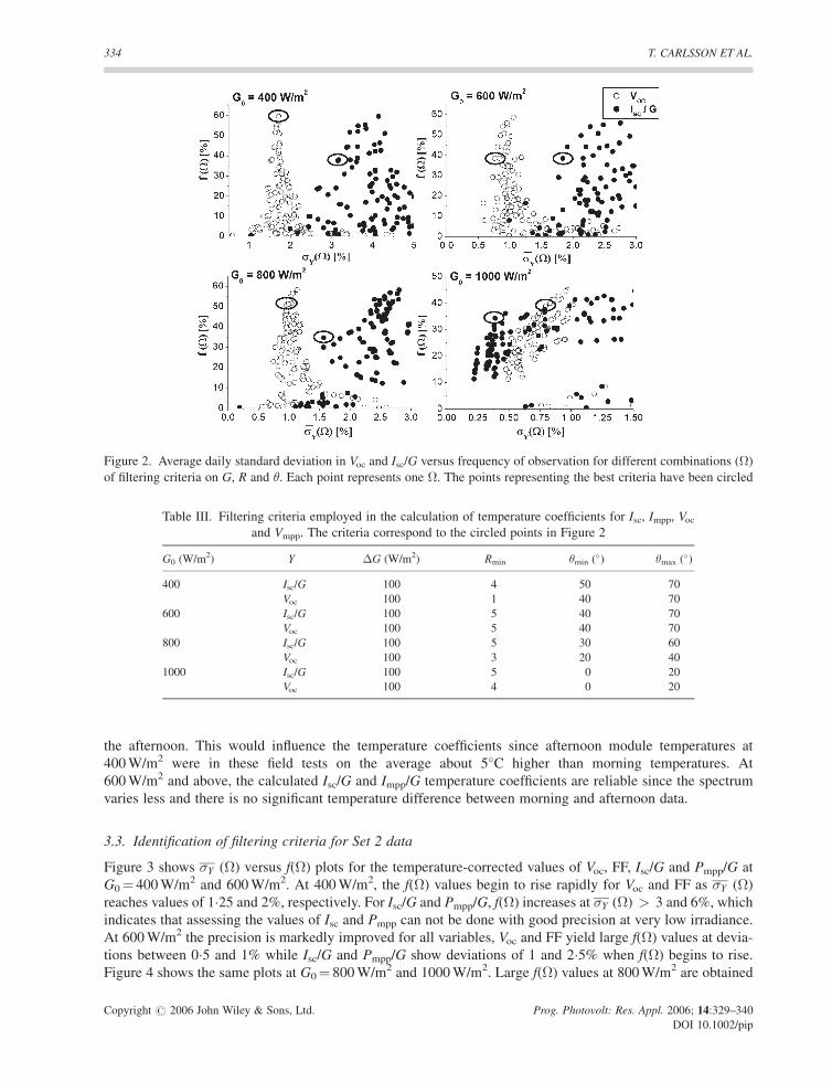
Selection of Set 1 data was done for two performance parameters, Voc and Isc/G. Temperature coefficients for

Vmpp and Impp/G were calculated from the same set of data as those of Voc and Isc/G, respectively. Figure 2 shows

�Y (�) versus f(�) for four values of G0. Some data points with high �Y (�) have been excluded from the figure

for clarity. It can be seen that �Y (�) is smaller for Voc than for Isc/G at every irradiance except 1000 W/m2. The

magnitude of �Y (�) decreases as a function of irradiance for both Voc and Isc/G. The points representing the �which were chosen for calculation of temperature coefficients have been encircled in Figure 2 and the filtering

criteria of these � are shown in Table III. The condition f(�)> 30% was used as the selection criterion together

with a small �Y (�) value.

3.2. Temperature coefficients

Filtering was performed on the data according to the conditions in Table III, and temperature coefficients were

calculated at each irradiance level from the filtered data set for Voc, Vmpp, Isc/G and Impp/G. Differences in coef-

ficients between modules were significant. Table IV shows, for each performance parameter, the average of the

coefficients and the standard deviation in the coefficients over all modules. It is worth noting that the irradiance

sensitivity of Isc/G and Impp/G adds significant uncertainty to their temperature coefficients at 400 W/m2 since

the analyzed data were primarily gathered early in the morning and late in the afternoon. Filtering based on R

may not limit the spectral variation sufficiently, and a small misalignment of the plane-of-array irradiance

sensor would create a systematic difference between Isc/G and Impp/G values measured in the morning and



DOI 10.1002/pip

the afternoon. This would influence the temperature coefficients since afternoon module temperatures at

400 W/m2 were in these field tests on the average about 5�C higher than morning temperatures. At

600 W/m2 and above, the calculated Isc/G and Impp/G temperature coefficients are reliable since the spectrum

varies less and there is no significant temperature difference between morning and afternoon data.

3.3. Identification of filtering criteria for Set 2 data

Figure 3 shows �Y (�) versus f(�) plots for the temperature-corrected values of Voc, FF, Isc/G and Pmpp/G at

G0¼ 400 W/m2 and 600 W/m2. At 400 W/m2, the f(�) values begin to rise rapidly for Voc and FF as �Y (�)

reaches values of 1�25 and 2%, respectively. For Isc/G and Pmpp/G, f(�) increases at �Y (�) > 3 and 6%, which

indicates that assessing the values of Isc and Pmpp can not be done with good precision at very low irradiance.

At 600 W/m2 the precision is markedly improved for all variables, Voc and FF yield large f(�) values at devia-

tions between 0�5 and 1% while Isc/G and Pmpp/G show deviations of 1 and 2�5% when f(�) begins to rise.

Figure 4 shows the same plots at G0¼ 800 W/m2 and 1000 W/m2. Large f(�) values at 800 W/m2 are obtained

Table III. Filtering criteria employed in the calculation of temperature coefficients for Isc, Impp, Voc

and Vmpp. The criteria correspond to the circled points in Figure 2

G0 (W/m2) Y �G (W/m2) Rmin �min (�) �max (�)

400 Isc/G 100 4 50 70

Voc 100 1 40 70

600 Isc/G 100 5 40 70

Voc 100 5 40 70

800 Isc/G 100 5 30 60

Voc 100 3 20 40

1000 Isc/G 100 5 0 20

Voc 100 4 0 20

Figure 2. Average daily standard deviation in Voc and Isc/G versus frequency of observation for different combinations (�)

of filtering criteria on G, R and �. Each point represents one �. The points representing the best criteria have been circled



DOI 10.1002/pip

when �Y (�) > 0�25–0�3% for Voc and FF, and when �Y (�) > 0�5% and �Y (�) > 1% for Isc/G and Pmpp/G,

respectively. At 1000 W/m2 the rise in f(�) occurs at �Y (�) ’ 0�1% for Voc and FF and �Y (�) ’ 0�2% for Isc/G

and Pmpp/G. In general, an increase of 200 W/m2 in the irradiance level gives a relative decrease in �Y (�) of

approximately 50%. For reasons to be explained later, a comparison between the data in Figures 3 and 4 with

Table I shows that many �FF values are lower than the estimated FF measurement error, and �Pmppvalues are

lower than the Pmpp error at 800 and 1000 W/m2.

Table IV. Temperature coefficient averages and standard deviation between

modules at four irradiance levels, calculated from Set 1 data. Isc/G and Impp/G

temperature coefficients at 400 W/m2 are subject to high uncertainty

G0 (W/m2) Y �Y average (%/�C) �Y stdev (%/�C)

400 Isc/G �0�167 0�123

Impp/G �0�155 0�167

Voc �0�321 0�042

Vmpp �0�317 0�128

600 Isc/G 0�036 0�048

Impp/G 0�068 0�072

Voc �0�321 0�038

Vmpp �0�363 0�077

800 Isc/G 0�058 0�032

Impp/G 0�066 0�061

Voc �0�328 0�028

Vmpp �0�400 0�054

1000 Isc/G 0�066 0�028

Impp/G 0�066 0�064

Voc �0�325 0�030

Vmpp �0�407 0�051

Figure 3. Average daily standard deviation of temperature-corrected performance parameters versus frequency of

observation for different combinations (�) of filtering criteria on G, T, R and � at G0¼ 400 W/m2 and 600 W/m2. Each point

represents one �. The points used in the method comparison for G0¼ 600 W/m2 have been encircled



DOI 10.1002/pip

3.4. Comparison between different methods for performance evaluation

In order to compare performance parameter predictions made with the method presented in this paper (referred

to as method A) to that which is obtained with a standard method which includes only minimal data filtering

(method B), the time series of the performance parameters measured from one randomly selected module were

calculated at irradiances of 600 W/m2 and 1000 W/m2 with both methods. The filtering conditions at 600 and

1000 W/m2 corresponding to the circled points in Figures 3 and 4 were chosen as the best ones based on the

selection criteria f(�) > 20% and a small �Y (�). The conditions corresponding to the circled points are pre-

sented in Table V. The selection was made only for parameters with �Y values larger than their measurement

error estimates. In method A, data filtering was performed according to these conditions and temperature cor-

rections were calculated with the module-specific temperature coefficients from Section 3.2. In method B, the

only filtering was performed in the selection of the analyzed data within an irradiance interval of � 50 W/m2

from the irradiance level under study. The temperature coefficients of the studied module were calculated in

method B for Isc/G, Impp/G, Voc and Vmpp at 1000 W/m2 by performing a linear fit corresponding to Equation

(1) to the entire data set and using 25�C as the reference temperature. These coefficients were assumed to be

Figure 4. Average daily standard deviation of temperature-corrected performance parameters versus frequency of

observation for different combinations (�) of filtering criteria on G, T, R and � at G0¼ 800 W/m2 and 1000 W/m2. Each point

represents one �. The points used in the method comparison for G0¼ 1000 W/m2 have been circled

Table V. The best filtering criteria at G0¼ 600 W/m2 and 1000 W/m2, which correspond to the circled points

in Figures 3 and 4

G0 (W/m2) Y �G (W/m2) Tmin (�C) Tmax (�C) Rmin �min (�) �max (�)

600 Voc 80 30 50 3 40 60

Isc/G 100 30 60 3 30 50

Pmpp 100 30 60 3 30 50

1000 Voc 100 30 60 4 0 10

Isc/G 100 30 60 5 0 10



DOI 10.1002/pip

independent of irradiance and were used at both 600 and 1000 W/m2. In both methods, a daily average of each

temperature-corrected performance parameter was calculated for all days with at least three measurements.

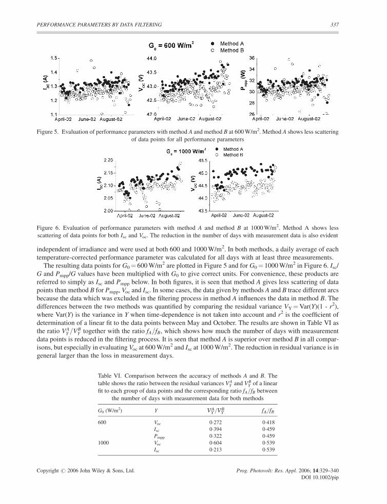
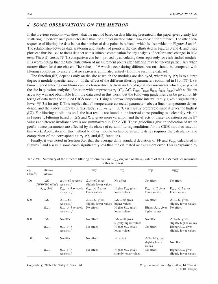
The resulting data points for G0¼ 600 W/m2 are plotted in Figure 5 and for G0¼ 1000 W/m2 in Figure 6. Isc/

G and Pmpp/G values have been multiplied with G0 to give correct units. For convenience, these products are

referred to simply as Isc and Pmpp below. In both figures, it is seen that method A gives less scattering of data

points than method B for Pmpp, Voc and Isc. In some cases, the data given by methods A and B trace different arcs

because the data which was excluded in the filtering process in method A influences the data in method B. The

differences between the two methods was quantified by comparing the residual variance VY¼Var(Y)(1 - r2),

where Var(Y) is the variance in Y when time-dependence is not taken into account and r2 is the coefficient of

determination of a linear fit to the data points between May and October. The results are shown in Table VI as

the ratio VAY =V

BY together with the ratio fA=fB, which shows how much the number of days with measurement

data points is reduced in the filtering process. It is seen that method A is superior over method B in all compar-

isons, but especially in evaluating Voc at 600 W/m2 and Isc at 1000 W/m2. The reduction in residual variance is in

general larger than the loss in measurement days.

Figure 5. Evaluation of performance parameters with method A and method B at 600 W/m2. Method A shows less scattering

of data points for all performance parameters

Figure 6. Evaluation of performance parameters with method A and method B at 1000 W/m2. Method A shows less

scattering of data points for both Isc and Voc. The reduction in the number of days with measurement data is also evident

Table VI. Comparison between the accuracy of methods A and B. The

table shows the ratio between the residual variances VAY and VB

Y of a linear

fit to each group of data points and the corresponding ratio fA=fB between

the number of days with measurement data for both methods

G0 (W/m2) Y VAY =V

BY fA=fB

600 Voc 0�272 0�418

Isc 0�394 0�459

Pmpp 0�322 0�459

1000 Voc 0�604 0�539

Isc 0�213 0�539



DOI 10.1002/pip

4. SOME OBSERVATIONS ON THE METHOD

In the previous section it was shown that the method based on data filtering presented in this paper gives clearly less

scattering in performance parameter data than the simpler method which was chosen for reference. The other con-

sequence of filtering the data is that the number of data points is reduced, which is also evident in Figures 5 and 6.

The relationship between data scattering and number of points is the one illustrated in Figures 3 and 4, and these

plots can thus be used to find a data set with a suitable combination for any analysis of performance changes in field

tests. The f(�) versus �Y (�) comparison can be improved by calculating them separately for each studied module.

It is worth noting that the time distribution of measurement points after filtering may be uneven particularly when

narrow filters for � are chosen. The values of � which occur during different seasons should be compared with

filtering conditions to ensure that no season is eliminated entirely from the resulting data set.

The function f(�) depends only on the site at which the modules are deployed, whereas �Y (�) is to a large

degree a module-specific function. If the effect of the different filtering parameters contained in � on �Y (�) is

known, good filtering conditions can be chosen directly from meteorological measurements which give f(�) at

the site in question analytical function which represents �Y (G0, �G, Tmin, Tmax, Rmin, �min, �max) with sufficient

accuracy was not obtainable from the data used in this work, but the following guidelines can be given for fil-

tering of data from the studied CIGS modules. Using a narrow temperature interval rarely gives a significantly

lower �Y (�) for any Y. This implies that all temperature-corrected parameters obey a linear temperature depen-

dence, and the widest interval (in this study; Tmax–Tmin¼ 30�C) is usually preferable since it gives the highest

f(�). For filtering conditions on �, the best results are found in the interval corresponding to a clear day, visible

in Figure 1. Filtering based on �G and Rmin gives more variation, and the effects of these two criteria on the �Y

values at different irradiance levels are summarized in Table VII. These guidelines give an indication of which

performance parameters are affected by the choice of certain filtering conditions for the CIGS modules tested in

this work. Application of this method to other module technologies and testsites requires the calculation and

comparison of the corresponding �Y (�) and f(�) functions.

Finally, it was noted in Section 3.3. that the average daily standard deviation of FF and Pmpp calculated in

Figures 3 and 4 was in some cases significantly less than the estimated measurement error. This is explained by

Table VII. Summary of the effect of filtering criteria �G and Rmin on f and on the �Y values of the CIGS modules measured

in this field test

G0 Filtering f �Voc�Isc

�FF �Pmpp

(W/m2) criterion

400 �G �G¼ 60 severely �G¼ 60 gives No effect No effect No effect

(60/80/100 W/m2) restricts f slightly lower values

Rmin (1–8) Rmin > 4 severely Rmin 4 2 gives Higher Rmin gives Rmin 4 2 gives Rmin 4 2 gives

restricts f lower values lower values lower values lower values

600 �G �G¼ 60 �G¼ 60 gives �G¼ 60 gives No effect �G¼ 60 gives

restricts f slightly lower values higher values slightly lower values

Rmin Rmin > 5 severely No effect Higher Rmin gives Higher Rmin gives No effect

restricts f lower values higher values

800 �G No effect No effect �G¼ 60 gives No effect �G¼ 60 gives

slightly higher values slightly higher values

Rmin Rmin > 6 No effect Higher Rmin gives No effect Higher Rmin gives

restricts f lower values slightly lower values

1000 �G No effect No effect No effect �G¼ 60 gives

slightly lower No effect

values

Rmin Rmin > 6 No effect Higher Rmin gives No effect Higher Rmin gives

restricts f slightly lower values slightly lower values



DOI 10.1002/pip

the operation of the electronic load used in scanning the I–V curves. For given irradiance level, the current–

voltage pairs on the I–V curve which are recorded in the measurement will be very nearly identical in different

I–V scans, which gives a low standard deviation and therefore an apparent accuracy higher than the real accu-

racy of the maximum power point determination. Within the limits set by the measurement equipment, the real

accuracy can be increased by increasing the number of measurement points. In the measurement set-up used in

this study, a quadrupling of the number of measurement points to 320 would have yielded error estimates from

the I–V analysis slightly below 0�5% for FF and 0�3% for Pmpp.

5. SUMMARY AND CONCLUSIONS

In this work, a data filtering methodology for improving the evaluation of performance parameters in field tested

PV modules was developed and applied to CIGS technology. The methodology is equally applicable to any PV

technology and it is a valuable tool in field testing since every analysis of PV field data must employ data filter-

ing to some degree and because it is equally applicable to any PV technology. Different filtering conditions were

compared to eachother based on how accurately a given performance parameter can be evaluated in the filtered

data set [�Y (�)] and how many days of data are available after filtering [f(�)]. The best filters are a matter of

subjective choice depending on the application. The choice of filters for the example presented in this paper

yielded, at an irradiance of 1000 W/m2, a 40% lower residual variance in Voc and a 79% lower residual variance

in Isc than what was obtained with a regular temperature and irradiance correction method. The number of days

with measurement data was reduced by 46% by the same filtering conditions. Medium irradiance (600 W/m2)

results showed reductions in the residual variance of Pmpp (68%), Isc (61%) and Voc (73%) significantly larger

than the loss of measurement days (54–58%). This shows that significant reductions of data scattering can be

obtained when the analysis is confined to specified intervals of basic meteorological and module parameters.

Results presented in this paper also show that the apparent accuracy (as represented by the standard deviation)

of fill factor and Pmpp measurements may be misleading if the number of I–V points gathered in the measurement

is insufficient. This should be taken into account in the planning of field test measurements. In conjunction with

the performance evaluation presented in this paper, a method for calculating temperature coefficients directly

from field measurement data was presented. Using time as an independent variable when a least squares fit is

performed reduces the time-dependent variation which would affect the fit strongly if data from a long time per-

iod is used. Reliable temperature coefficients for voltage parameters can be obtained at plane-of-array irradiances

as low as 400 W/m2, whereas for current parameters 600 W/m2 was the practical lower limit in this study.

With the help of the methodology presented in this paper, changes in the performance of field tested modules

can be detected with greater accuracy than with methods which employ only minimal filtering of data. This not

only makes it possible to detect changes at an earlier stage of testing, but also facilitates better comparisons

between observed changes in performance parameters and measured stress factors such as high module tem-

perature peaks, temperature cycles or unusually high insolation. If correlations between stress factors and per-

formance changes are found, the necessary feedback for accelerated ageing tests in the laboratory can be given

directly and future module designs improved.

Acknowledgements

Svenska Litteratursallskapet i Finland rf is gratefully acknowledged for financial support.

NOMENCLATURE

AY zero order time dependence coefficient for YREF

BY first order time dependence coefficient for YREF

CY second order time dependence coefficient for YREF

d general symbol for any day

f proportion of days with data available, a function of �fA proportion of days with data available, method A



DOI 10.1002/pip

fB proportion of days with data available, method B

FF fill factor

G plane-of-array irradiance (W/m2)

GD diffuse horizontal irradiance (W/m2)

GH global horizontal irradiance (W/m2)

Gmax maximum plane-of-array irradiance (W/m2)

G0 plane-of-array irradiance filtering parameter (W/m2)

�G plane-of-array irradiance interval filtering parameter (W/m2)

Impp maximum power point current (A)

Isc short-circuit current (A)

m general symbol for any module

Pmpp maximum module power (W)

R GH/GD ratio

Rmin GH/GD ratio filtering parameter

r2 coefficient of determination

SS sum of squares

T module temperature (�C)

Tmax module temperature filtering parameter (�C)

Tmin module temperature filtering parameter (�C)

t time (months)

TREF reference temperature (�C)

Vmpp maximum power point voltage (V)

Voc open-circuit voltage (V)

VY residual variance in Y

VYA residual variance in Y obtained with method A

VYB residual variance in Y obtained with method B

Var variance

Y general symbol for Impp, Vmpp, Isc, Voc, Impp/G or Isc/G

YREF value of Y at reference conditions

�Y temperature coefficient of Y (%/�C)

�Y (�,m,d) module- and day-specific standard deviation in Y with filter � (%)

�Y (�,m) average of �Y(�,m,d) over all days (%)

�Y (�) average of �Y (�,m) over all modules (%)

� sunlight angle of incidence (�)�max sunlight angle of incidence filtering parameter (�)�min sunlight angle of incidence filtering parameter (�)� a specified combination of filtering criteria

REFERENCES

1. Czanderna A, Jorgensen G. Accelerated life testing and service lifetime prediction for PV technologies in the twenty-

first century. Electrochemical Society Proceedings 99-11 (Photovoltaics for the 21st century) 1999; 57–67.

2. McMahon T. Accelerated testing and failure of thin-film PV modules. Progress in Photovoltaics: Research and

Applications 2004; 12(2–3): 235–248. DOI: 10.1002/pip.526

3. King D, Kratochvil J, Boyson W. Temperature coefficients for PV modules and arrays: measurement methods,

difficulties and results. Proceedings of the 26th IEEE PVSC 1997; 1183–1186.

4. Kurtz S, Myers D, Townsend T, Whitaker C, Maish A, Hulstrom A, Emery K. Outdoor rating conditions for photovoltaic

modules and systems. Solar Energy Materials and Solar Cells 2000; 62(4): 379–391.

5. Mohring H-D, Stellbogen D, Schaffler R, Oelting S, Gegenwart R, Konttinen P, Carlsson T, Cendagorta M, Herrmann W.

Outdoor performance of polycrystalline thin film PV modules in different European climates. Proceedings of the 19th

European Photovoltaic Solar Energy Conference, 2004: 2098–2101.



DOI 10.1002/pip

Documents

Data filtering methods for determining performance parameters in photovoltaic module field tests