Data Limited Techniques for Tier 4 Stocks: An …sedarweb.org/docs/wsupp/S46_RD_08_Black Sea Bass_Mid-AtlSSC.pdf · setting harvest control rules using closed loop simulations for

DataLimitedTechniquesforTier4Stocks:Analternativeapproachto

settingharvestcontrolrulesusingclosedloopsimulationsformanagementstrategyevaluation

JasonMcNamee,GavinFay,andStevenCadrin

SEDAR46-RD-08

February2016

Data Limited Techniques for Tier 4 Stocks:

An alternative approach to setting harvest

control rules using closed loop simulations

for management strategy evaluation

Jason McNamee: RI Division of Fish and Wildlife

Gavin Fay: University of Massachusetts Dartmouth

Steven Cadrin: University of Massachusetts Dartmouth

Introduction

The Mid-Atlantic Scientific and Statistical Committee (SSC) uses a classification system for

managing the information on the marine resources that they are responsible for. This

classification system categorizes the information, usually in the form of an analytical stock

assessment, in to one of four tiers. The tier used to categorize information useful for setting an

overfishing limit (OFL) when an analytical assessment is not available is referred to as tier 4.

Under tier 4, the SSC uses a pre-defined method of setting a constant catch value. The constant

catch that is defined is taken from the catch that was achieved during a period of time where the

SSC believes the stock was rebuilding and is therefore believed to be a safe harvest level

(Carmichael and Fenske 2011).

Performance evaluations of constant catch control rules for data-limited stocks suggests that they

may be sustainable, but not necessarily a good proxy for maximum sustainable yield (ICES

2012; Geromont and Butterworth 2014; Carruthers et al. 2014). With a constant catch approach

there are issues that arise as a population rebounds, where potential yield will be foregone if that

constant catch value is set too low, and conversely if a population declines, the constant catch

approach could lead to overharvest unless the constant catch value is adjusted down. The

following analysis seeks to provide an alternative approach for use on tier 4 stocks that is

performance tested, dynamic, straightforward, rapid to implement, and which offers a

comparative analysis of harvest control rule approaches that can be used in situations where data

are lacking or are not accepted by the SSC for specification setting.

Analytical stock assessments are the usual basis for estimating an OFL. In many cases fisheries

lack the data necessary to support a conventional stock assessment, requiring the use of methods

that can be used in data- or analysis-limited situations. Even if a fishery has ample data and

research, there are situations where an analytical assessment is not possible due to external

constraints, such as not enough human resources to perform the analysis or a lack of economic

incentives to devote an analyst’s time to developing a comprehensive assessment. Finally,

sometimes an analytical assessment exists, but is not useful for specification setting due to not

passing peer review or not being accepted due to diagnostic issues. This latter situation is the

case for black sea bass, the focus of this work.

Management strategy evaluation (MSE) is a technique that can be used to evaluate and compare

the performance of assessment and management methods (Bunnefeld et al. 2011). Simulating the

behavior of harvest control rules through MSE and then using this information to evaluate the

performance of a set of methods allows for an objective way to consider trade-offs among

management objectives (Wetzel and Punt 2011; Wilberg et al. 2011, Geromont and Butterworth

2014; Carruthers et al. 2014). The following analysis uses an MSE approach as developed by

Carruthers et al. (2014) to evaluate the relative performance of a suite of data limited analytical

techniques for black sea bass. This approach may offer the SSC an alternative to the current

approach for tier 4 stocks. The application to black sea bass may also provide a framework for

specification setting until an approved analytical assessment can be accomplished.

Methods

The procedures as defined by Carruthers et al. (2014) were used for this analysis. This procedure

is implemented through the use of an application developed for the R statistical software package

(R Core Team 2014) through the R package “DLMtool” (Carruthers 2015). This package

provides flexible specification of an operating model of population dynamics of a fished stock,

effort dynamics of a targeted fishery, an observation model that can reflect biases and

imprecision associated with monitoring data, and a set of stock assessment methods and harvest

control rules that determine management advice fed back into the operating model. Although the

dynamics of the black sea bass fishery were not exactly represented, the models underlying

DLMtool provide a flexible and comprehensive framework for comparing assessment and

control rule performance across a range of uncertainties. We therefore use this package to

emulate and evaluate plausible behavior given dynamics and uncertainties that are characteristic

of black sea bass.

A black sea bass specific operating model, which is a set of biological and fishery specific

parameters for the black sea bass fishery, was developed. The operating model was created using

information generated from the last peer reviewed stock assessment for black sea bass (NEFSC

2012), and assuming reasonable estimates for the degree of uncertainty around parameters when

no specific information on uncertainty were available (uncertainty estimates are needed for the

stochastic implementation of the MSE procedure). The information that is available to the

assessment and control rule procedures is determined by an observation model. The parameters

for the observation model were specified to allow for simulated data to be both imprecise and

possibly biased, appropriately reflecting the nature of monitoring data.

The operating model includes numerous uncertainties that are tested through the MSE procedure.

Some of the most important uncertainties tested for the black sea bass case were natural

mortality (M), steepness of the spawner-recruit relationship (h), depletion of the stock (D),

vulnerability of the oldest age class (Vmaxage), spatial targeting of the stock (Spat_targ), and a

hyperstability parameter for the fishery independent information (beta). These uncertainties were

all tested with a range of point estimate values as well as adequate ranges for their associated

uncertainties (Table 1). Other input parameters that are used by the various procedures are better

supported by research, including Von Bertalanffy equation parameters, length weight

parameters, maximum age, and age at first capture, so were treated with appropriate levels of

uncertainty. All of the uncertainties included in the operating model become the framework that

the MSE samples within, and allows for testing of the most important uncertainties for each

specific procedure.

The operating model was run through a closed loop MSE procedure, and a set of appropriate

analytical assessment methods and harvest control rules (procedures) were identified and

compared. Two separate effort scenarios were tested, one referred to as “flat effort”, which

allows for trends through time to be both negative and positive, and “increasing effort”, which

only allows for a positive trend in effort through time. These procedures were then filtered based

on a set of performance criteria that were meant to mimic management objectives. The criteria

used were yield, probability of overfishing, and the probability of depleting the stock to low

abundance (10% of BMSY). Each MSE was run twice to compare the stability of the simulation.

In addition to the built-in procedures in the DLMtool package, two additional procedures were

developed that are based on observations of the historical exploitation of the stock, one that uses

a reference slope of the exploitation rate index and one that uses a target exploitation rate index.

These additional procedures were also run through the MSE and compared to the other

procedures. The code for these additional procedures can be viewed in Appendix 1.

Methodology for all other procedures can be viewed by typing the procedure name in to the R

statistical environment with the DLMtool package loaded.

Once a set of appropriate procedures were determined based on the closed loop MSE, an

additional analysis was run on actual data for black sea bass. These data were derived from

recent fishery statistics on catch, information from appropriate fishery independent surveys, and

information from the last stock assessment for black sea bass (NEFSC 2012). Fishery

independent information used was the spring index of the National Marine Fisheries Service

(NMFS) trawl survey. This index was selected as the most defensible for this exercise as the

survey takes place during a period of time in which the black sea bass population is undergoing

its seasonal migration so is most likely susceptible to trawl gear, is in general representing only

fish older than 1 year, and spans the entire extent of the known northern stock range (NEFSC

2012).

From the real dataset, overfishing levels (OFLs) for black sea bass are produced based on the

chosen management procedures and preferred options are offered for consideration. A procedure

similar to that currently used by the SSC is also offered for comparative review with the chosen

approaches.

Results

MSE

Using the operating model as described above, an MSE was run to determine the best procedures

to use for the black sea bass case. For the full list of approaches, see the DLMtool package

information (Carruthers 2015). From a suite of 47 different data limited procedures available in

the DLMtool package, the approaches were narrowed down based on the outcome of the MSE.

The approaches were narrowed based on a set of criteria that are meant to mimic management

objectives such as minimizing the probability of overfishing, optimizing yield, and minimizing

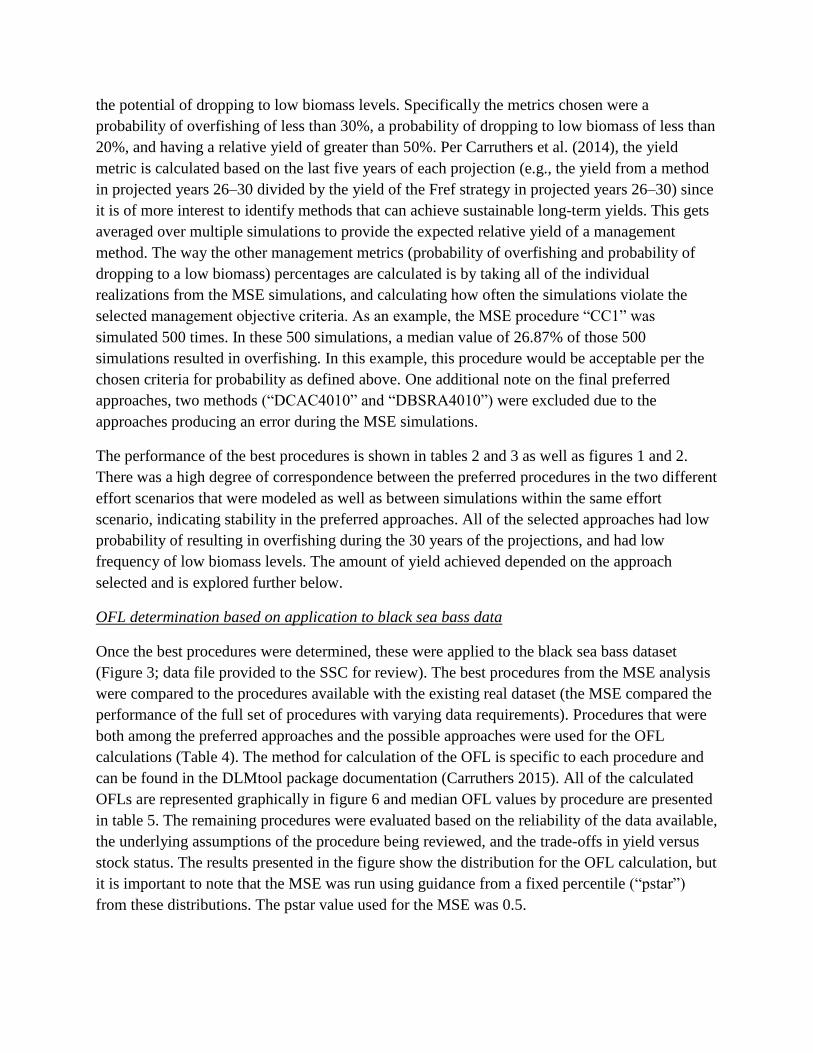
the potential of dropping to low biomass levels. Specifically the metrics chosen were a

probability of overfishing of less than 30%, a probability of dropping to low biomass of less than

20%, and having a relative yield of greater than 50%. Per Carruthers et al. (2014), the yield

metric is calculated based on the last five years of each projection (e.g., the yield from a method

in projected years 26–30 divided by the yield of the Fref strategy in projected years 26–30) since

it is of more interest to identify methods that can achieve sustainable long-term yields. This gets

averaged over multiple simulations to provide the expected relative yield of a management

method. The way the other management metrics (probability of overfishing and probability of

dropping to a low biomass) percentages are calculated is by taking all of the individual

realizations from the MSE simulations, and calculating how often the simulations violate the

selected management objective criteria. As an example, the MSE procedure “CC1” was

simulated 500 times. In these 500 simulations, a median value of 26.87% of those 500

simulations resulted in overfishing. In this example, this procedure would be acceptable per the

chosen criteria for probability as defined above. One additional note on the final preferred

approaches, two methods (“DCAC4010” and “DBSRA4010”) were excluded due to the

approaches producing an error during the MSE simulations.

The performance of the best procedures is shown in tables 2 and 3 as well as figures 1 and 2.

There was a high degree of correspondence between the preferred procedures in the two different

effort scenarios that were modeled as well as between simulations within the same effort

scenario, indicating stability in the preferred approaches. All of the selected approaches had low

probability of resulting in overfishing during the 30 years of the projections, and had low

frequency of low biomass levels. The amount of yield achieved depended on the approach

selected and is explored further below.

OFL determination based on application to black sea bass data

Once the best procedures were determined, these were applied to the black sea bass dataset

(Figure 3; data file provided to the SSC for review). The best procedures from the MSE analysis

were compared to the procedures available with the existing real dataset (the MSE compared the

performance of the full set of procedures with varying data requirements). Procedures that were

both among the preferred approaches and the possible approaches were used for the OFL

calculations (Table 4). The method for calculation of the OFL is specific to each procedure and

can be found in the DLMtool package documentation (Carruthers 2015). All of the calculated

OFLs are represented graphically in figure 6 and median OFL values by procedure are presented

in table 5. The remaining procedures were evaluated based on the reliability of the data available,

the underlying assumptions of the procedure being reviewed, and the trade-offs in yield versus

stock status. The results presented in the figure show the distribution for the OFL calculation, but

it is important to note that the MSE was run using guidance from a fixed percentile (“pstar”)

from these distributions. The pstar value used for the MSE was 0.5.

Discussion

One of the goals of this exercise was to analyze a set of harvest control rules and compare that to

the current harvest control rule employed by the SSC for tier 4 stocks. The procedure in the

DLMtool package that is closest to the procedure currently used by the SSC is named “CC1” and

is a procedure that uses a constant catch from a set number of years. This procedure is not

exactly as that used by the SSC, but is a reasonable proxy for comparison. This analysis indicates

that the static constant catch approaches are not the best procedures as they can lead to foregone

yield and higher probabilities of overfishing (Figures 1 and 2). ICES (2012) evaluations of data-

limited harvest control rules found similar performance of constant catch scenarios, in which

fisheries were sustainable, but low stocks remained low, and high stocks remained high. This

general result also corroborates the analysis as noted in Geromont and Butterworth (2014), where

they determined that the use of a constant catch procedure with no feedback control was not a

preferred option. Carruthers et al. (2014) also arrived at the same conclusion about static catch

based approaches, finding them to have poorer performance with realized yield and greater

probabilities of overfishing than other more dynamic approaches.

The usefulness of depletion based approaches (e.g. DCAC, DBSRA) was downgraded for the

black sea bass case, because they are sensitive to the initial estimate of depletion, creating a need

to be very cautious with the estimate, which can lead to the potential of foregone yield. In

addition, the assumption of the stock being in an unfished state in the initial years is also violated

for the black sea bass case, another assumption violation of these approaches (Dick and MacCall

2010). The catch stream chosen for this analysis starts in 1982 as this is the period of time where

recreational catch information has been systematically collected. Recreational harvest makes up

a large proportion of black sea bass removals, and therefore is an important source of removals

to account for. The stock was already exploited during this time period. In addition to the issues

with the underlying assumptions, sensitivity analysis indicates that the performance of the

different harvest control rule procedures is fairly robust to most of the operating model inputs,

the main exception being the choice in stock depletion level, which can have significant impacts

on the outcomes of the MSE (Figure 7). The depletion based approaches may be viable for other

tier 4 stocks, in particular if the stock is believe to be newly exploited. Carruthers et al (2014)

also found that the depletion methods they tested performed well when the depletion assumption

was reasonably close to actual depletion.

As noted above, the procedures were all robust to the operating model inputs. Plots of the effect

of varying input values for a set of important uncertainties is shown in figure 7. The exception to

this robustness was found in the depletion values, which did have a significant impact on relative

yield, probability of biomass dropping below 50% of BMSY, and overfishing. Beyond the

depletion input value, the rest of the parameters did not show dramatic changes in outcomes for

the ranges of values used in this analysis. One note that is important, the steepness (h) values

used for the analysis were chosen to be low. This was due to the finding that the steepness

parameter was causing errors in the MSE process for some of the simulations. These steepness

values could be examined further, but for the input values used for this analysis, it did not impact

the outcome of the MSE to a large degree.

One procedure that offered a good balance given the trade-offs between yield, overfishing

probability, and probability of dropping to a low stock size, as well as the characteristics of the

species and the reliability of the data available is the approach referred to as “GB_slope” in

Carruthers (2015). This approach uses the slope of recent estimates of abundance to determine

catch advice, with the aim of obtaining stable catch rates, and is similar to an approach from

Geromont and Butterworth (2014). This previous work also regarded this approach as one that

performed well given the tradeoffs that were considered. It is important to note that Little et al.

(2011) showed that this type of method only performs well if the recent average catch rate is

about the same as that expected at BMSY (for yield), or when F is below FMSY (for

overfishing). This may be the case for black sea bass given information from recent analytical

assessments on the stock as well as high indices of abundance found in many state surveys and

anecdotal reports of high catch in particular in the northern stretches of the stocks range. While

the “GB_slope” procedure offers a good balance of yield and risk, additional procedures

analyzed also indicated good long term yield while maintaining a low probability of overfishing

or dropping to a low stock size, and could also be useful for specification setting.

One extension of this analysis that could be considered for the black sea bass case would be to

use more fishery independent information in the analysis. This analysis chose a single fishery

independent index (namely the NMFS trawl survey spring index) as the most defensible source

of information at present, but other sources of fishery independent information exists as well, in

particular from state run fishery independent surveys. Approaches could be developed that

combine indices through approaches such as using a hierarchical modeling approach as

developed by Paul Conn (Conn 2010), or by weighting the surveys through an areal extent

approach. These analyses could provide a more robust estimate of population abundance

information that may not be as subject to large swings in abundance estimates from year to year.

An important final note for this analysis is that this is offered as an approach to consider for the

SSCs tier 4 stocks. In the specific case of black sea bass, this approach is only offered as a

potential interim solution for specification setting, as a full analytical assessment process is

underway for this stock. This full analytical assessment is being performed by the analysts from

this work along with other partners in black sea bass fishery science. Therefore these data limited

approaches should not be considered to the exclusion of a full analytical assessment. These

alternatives are provided for consideration as approaches to accommodate the period of time

before a full analytical assessment is peer reviewed and approved for management use for black

sea bass. It is further hoped that this approach can be applied beyond the black sea bass case to

help with the SSCs work on existing and future tier 4 stocks.

References

Bunnefeld, N, Hoshino, E, and Milner-Gulland, E. 2011. Management strategy evaluation: a

powerful tool for conservation? Trends in Ecology and Evolution, 26(9), pp. 441-447.

Carmichael, J., and K. Fenske (editors). 2011. Third National Meeting of the Regional Fisheries

Management Councils’ Scientific and Statistical Committees. Report of a National SSC

Workshop on ABC Control Rule Implementation and Peer Review Procedures. South Atlantic

Fishery Management Council, Charleston, October 19-21, 2010.

Carruthers, T, Punt, A, Walters, C, MacCall, A, McAllister, M, Dick, E, Cope, J. 2014.

Evaluating methods for setting catch limits in data-limited fisheries. Fisheries Research. 153: 48

– 68.

Carruthers, T. 2015. DLMtool: Data-Limited Methods Toolkit. R package version 1.35

http://CRAN.R-project.org/package=DLMtool.

Conn, P. 2010. Hierarchical analysis of multiple noisy abundance indices. Can. J. Fish. Aquat.

Sci. 67: 108–120.

Dick, E and MacCall, A. 2010. Estimates of sustainable yield for 50 data-poor stocks in the

Pacific Coast groundfish fishery management plan. NOAA Technical Memorandum. NOAA-

TM-NMFS-SWFSC-460.

Geromont, H, Butterworth, D. 2014. Generic management procedures for data-poor fisheries:

forecasting with few data. ICES Journal of Marine Science, doi:10.1093/icesjms/fst232

ICES. 2012. Report of the Workshop on the Development of Assessments based on LIFE history

traits and Exploitation Characteristics (WKLIFE), 13–17 February 2012, Lisbon, Portugal . ICES

CM 2012/ACOM:36. 122 pp.

Little, R, Wayte, S, Tuck, G, Smith, A, Klaer, N, Haddon, M, Punt, A, Thomson, R, Day, J,

Fuller, M. 2011. Development and evaluation of a cpue-based harvest control rule for the

southern and eastern scalefish and shark fishery of Australia. ICES Journal of Marine. Vol. 68

Issue 8, p1699-1705. 7p.

Northeast Fisheries Science Center (NEFSC). 2012. 53rd Northeast Regional Stock Assessment

Workshop (53rd SAW) Assessment Report. US Dept Commer, Northeast Fish Sci Cent Ref Doc.

12-05; 559 p.

R Core Team. 2014. R: A language and environment for statistical computing. R Foundation for

Statistical Computing, Vienna, Austria. URL http://www.R-project.org/.

Wetzel, C.R., Punt, A.E. 2011. Performance of a fisheries catch-at-age model (stock synthesis) in

data-limited situations. Mar. Freshw. Res. 62, 927–936.

http://cran.r-project.org/package=DLMtool

http://www.r-project.org/

Wilberg, M.J., Miller, T.J., Wiedenmann, J. 2011. Evaluation of Acceptable Biological Catch

(ABC) control rules for Mid-Atlantic stocks. Report to the Mid- Atlantic Fishery Management

Council. UMCES, CBL 11-029. Technical Report Series No. TS-622-11.

http://www.mafmc.org/meeting materials/SSC/2012-

03/Final%20MAFMC%20Report%20revised.pdf

Tables

Table 1 – Parameter values and uncertainties used for the operating model: natural mortality (M),

steepness of the spawner-recruit relationship (h), depletion of the stock (D), vulnerability of the

oldest age class (Vmaxage), spatial targeting of the stock (Spat_targ), and a hyperstability

parameter for the fishery independent information (beta), Von Bertalanffy Parameters (K, t0,

Linf), maximum age (maxage), length weight parameters (a, b), observation error in catch (Cobs)

and fishery independent index (Iobs). Full information on all inputs can be found in Appendix 1.

Parameter Value or Range

of Values

Associated CV or

Bias Estimate

Source

M 0.2 – 0.5 0.0 – 0.2 NEFSC 2012

h 0.3 – 0.4 0.3 NEFSC 2012

D 0.3 – 0.7 0.2 – 0.3 Reasonable Estimate

Vmaxage 0.4 – 1 NA Reasonable Estimate

Spat_targ -0.5 – 3 NA Reasonable Estimate

beta 0.333 – 3 NA Reasonable Estimate

K 0.17 – 0.22 0.0 – 0.03 NEFSC 2012

t0 0.14 – 0.19 NA NEFSC 2012

maxage

20 0.3

Dery and Mayo

(http://www.nefsc.noaa.gov/fbp/age-

man/bsb/bsb.htm)

Linf 62 - 70 0.0 – 0.03 NEFSC 2012

a 0.0000108 NA NEFSC 2012

b 3.0595 NA NEFSC 2012

ageM 4 – 6 1 NEFSC 2012

Cobs NA 0.2 – 0.4 Reasonable Estimate

Iobs NA 0.2 – 0.4 Reasonable Estimate

Table 2 – Best performing procedures and their performance for the “flat effort” scenario. Values

presented are median percentage values. POF = Probability of overfishing; P10 = Probability of

dropping below 10% BMSY; P50 = Probability of dropping below 50% BMSY; P100 =

Probability of dropping below BMSY

Method Yield POF P10 P50 P100

CC1 61.4 27.31 12.28 18.92 27.85

DCAC 83.35 12.65 3.37 8.47 17.28

DCAC_40 79.46 12.63 3.41 8.55 17.27

DynF 72.44 0.19 0.91 5.73 14.39

Fadapt 79.44 0.01 0.89 5.61 14.25

Fdem 120.12 3.07 1.27 8.14 19.25

FMSYref 150.32 8.1 2.4 12.89 25.77

FMSYref50 127.73 0 1.33 7.7 18.57

FMSYref75 146.09 0.22 1.75 10.37 22.08

Fratio 59.05 0 0.87 5.19 13.77

GB_slope 62.07 27.97 13.54 20.4 29.09

Gcontrol 54.88 22.98 12.08 18.19 26.73

Islope1 60.46 11.05 3.32 8.23 16.71

Rcontrol 39.84 27.17 13.16 20.91 30.04

SBT1 59.61 27.83 13.59 20.36 28.9

SPMSY 45.82 9.21 3.55 8.41 16.75

matsizlim 70.7 16.88 2.04 7.34 16.04

area1MPA 56.13 5.41 0.85 6.05 14.6

Table 3 – Best performing procedures and their performance for the “increasing effort” scenario.

Values presented are median percentage values. POF = Probability of overfishing; P10 =

Probability of dropping below 10% BMSY; P50 = Probability of dropping below 50% BMSY;

P100 = Probability of dropping below BMSY

Method Yield POF P10 P50 P100

CC4 52.88 11.91 6.02 11.93 19.64

DCAC 63.77 12.3 4.5 10.4 18.44

DCAC_40 62.1 11.67 4.47 10.38 18.44

DD 54.51 27.32 10.63 19.91 29.87

DynF 65.73 0.18 2.52 7.73 15.91

Fadapt 73.43 0.01 2.54 7.72 15.74

Fdem 111.17 1.73 2.92 10.02 18.99

FMSYref 143.88 7.64 3.78 14.07 24.97

FMSYref50 120.94 0 2.95 9.85 18.66

FMSYref75 139.18 0.23 3.32 12.06 21.61

Fratio 53.14 0 2.45 7.51 15.15

Gcontrol 77.64 26.55 16.87 24.16 32.01

Islope1 55.39 15.17 5.85 12.07 20.45

Islope4 48.64 6.8 3.7 9.13 16.71

SPMSY 38.06 10.5 5.81 11.63 19.28

matsizlim 71.7 26.73 5.03 11.87 20.74

area1MPA 56.42 9.67 2.57 9.17 17.86

Table 4 – Methods that overlapped between the preferred approaches as determined by the MSE

analysis and the methods possible given the real dataset used for black sea bass.

Overlapping Methods Used for OFL Calculations

CC1

DCAC

DCAC_40

DD

DynF

Fadapt

Fdem

Fratio

GB_CC

GB_slope

Gcontrol

Islope1

SBT1

SPMSY

SPslope

Rcontrol

CC4

Table 5 – Median OFL calculation for the various methods in metric tons.

Methods Median OFL Calculation (MT)

CC1 2,496

DCAC 2,526

DCAC_40 2,481

DD 3,898

DynF 1,108

Fadapt 6,237

Fdem 6,988

Fratio 3,002

Islope1 2,710

GB_CC 3,731

GB_slope 3,797

Gcontrol 1,519

SBT1 3,091

SPMSY 4,111

SPslope 2,354

Rcontrol 4,248

CC4 1,744

Figures

Figure 1 – Trade-off plots of the MSE for each of the procedures used for the “flat effort” simulations.

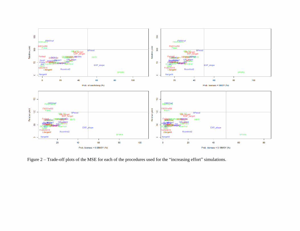
Figure 2 – Trade-off plots of the MSE for each of the procedures used for the “increasing effort” simulations.

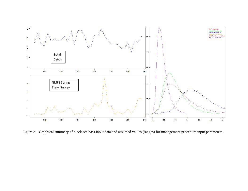
Figure 3 – Graphical summary of black sea bass input data and assumed values (ranges) for management procedure input parameters.

Total

Catch

NMFS Spring

Trawl Survey

Figure 6 – Calculated OFLs for all approaches.

Figure 7a – Sensitivity of the procedures to the beta parameter

Figure 7b – Sensitivity of the procedures to the Prob_staying parameter

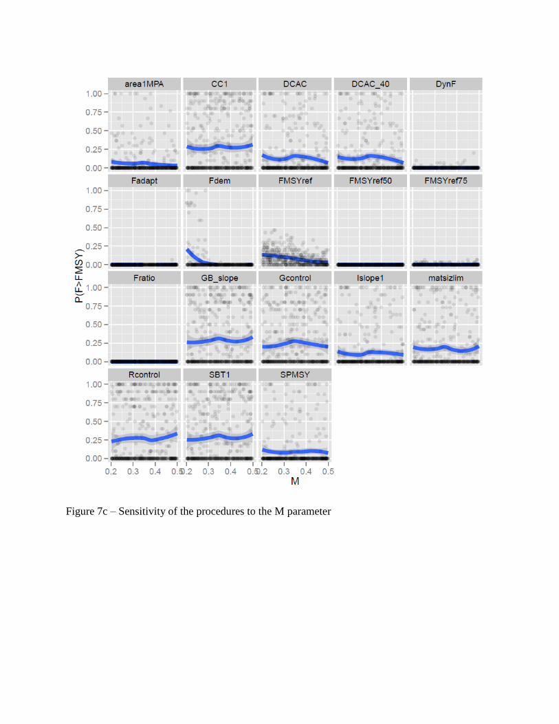
Figure 7c – Sensitivity of the procedures to the M parameter

Figure 7d – Sensitivity of the procedures to the Depletion parameter

Figure 7e – Sensitivity of the procedures to the h parameter

Figure 7f – Sensitivity of the procedures to the Spat_targ parameter

Figure 7g – Sensitivity of the procedures to the Vmaxage parameter

Figure 7h – Sensitivity of the procedures to the ageM parameter

Figure 7i – Sensitivity of the procedures to the beta parameter

Figure 7j – Sensitivity of the procedures to the Prob_staying parameter

Figure 7k – Sensitivity of the procedures to the M parameter

Figure 7l – Sensitivity of the procedures to the Depletion parameter

Figure 7m – Sensitivity of the procedures to the h parameter

Figure 7n– Sensitivity of the procedures to the Spat_targ parameter

Figure 7o – Sensitivity of the procedures to the Vmaxage parameter

Figure 7p – Sensitivity of the procedures to the ageM parameter

Figure 7q – Sensitivity of the procedures to the beta parameter

Figure 7r – Sensitivity of the procedures to the Prob_staying parameter

Figure 7s – Sensitivity of the procedures to the M parameter

Figure 7t – Sensitivity of the procedures to the Depletion parameter

Figure 7u – Sensitivity of the procedures to the h parameter

Figure 7v – Sensitivity of the procedures to the Spat_targ parameter

Figure 7w – Sensitivity of the procedures to the Vmaxage parameter

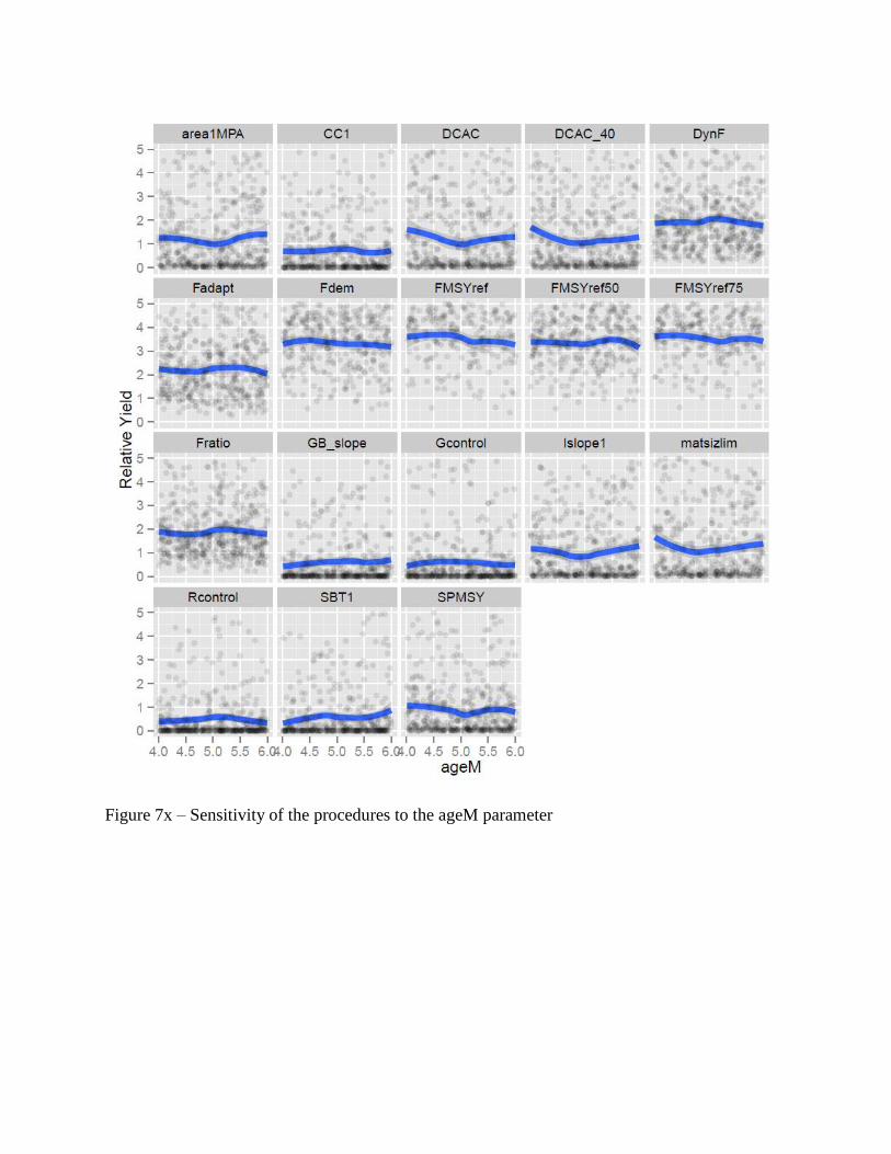
Figure 7x – Sensitivity of the procedures to the ageM parameter

Appendix 1 – Model code

##################################################################################

# Black sea bass data-limited / moderate assessments and MSE #

# 07/10/2015 #

# Code adapted from Carruthers (2015) #

# Jason McNamee, Gavin Fay, Steven Cadrin #

##################################################################################

##################################################################################

# needed commands for startup #

##################################################################################

library(DLMtool)

for(i in 1:length(DLMdat))assign(DLMdat[[i]]@Name,DLMdat[[i]])

sfInit(parallel=T,cpus=8)

sfExportAll()

set.seed(1)

##################################################################################

# Create Black sea bass stock object for MSE #

# Use Porgy and then modify parameters to fit our case #

##################################################################################

##Call in Porgy to use as stock object template

ourstock<-Porgy

###Modify to fit black sea bass case, info of source next to each parameter###

ourstock@Name<-"Black Sea Bass"

ourstock@maxage<-20 #max age at 20 from Dery and Mayo (http://www.nefsc.noaa.gov/fbp/age-

man/bsb/bsb.htm)

ourstock@R0<-10000000 # unfished recruitment; arbitrary, set it at value higher than highest catch value

seen in MT

ourstock@M<-c(0.2,0.5) #M between 0.2 and 0.5, based on 2012 assessment (SARC 53)

ourstock@Msd<-c(0.0, 0.2) #interannual variation in M, expressed as CV, used reasonable estimate

ourstock@Mgrad<-c(-0.2, 0.2) #temporal change in M, expressed as a percent

ourstock@h<-c(0.3, 0.4) #c(0.5, 0.99) #steepness, started with estimates based on SARC 53, but had to

adjust down due to errors with DBSRA

ourstock@SRrel<-1 #spawner recruit relationship, set to BH=1, Ricker is 2

ourstock@Linf<-c(62,70) #Von B Linf param, bounded by info in 2012 assessment

ourstock@K<-c(0.17,0.22) #Von B K parameter, bounded by info in 2012 assessment

ourstock@t0<-c(0.14,0.19) #Von B t0 param, bounded by info in 2012 assessment

ourstock@Ksd<-c(0.0,0.03) #interannual variability in K parameter, bounded by reasonable estimate

ourstock@Kgrad<-c(-0.2, 0.2) #temporal trend in K parameter, expressed as percent

ourstock@Linfsd<-c(0.0,0.03) #interannual variability in Linf param, bounded by reasonable estimate

ourstock@Linfgrad<-c(-0.25,0.25) #mean temporal trend in Linf param, bounded by reasonable estimate

ourstock@recgrad<-c(-10,10) #mean temporal trend in lognormal rec devs, resonable est

ourstock@AC<-c(0.1, 0.9) #Autocorrelation in recruitment deviations rec(t)=AC*rec(t-1)+(1-AC)*sigma(t)

ourstock@a<- 0.0000108 #Length-weight parameter alpha (note should not be in logspace, info from Gary S

see expl spreadsheet)

ourstock@b<- 3.0595 #Length-weight parameter beta

ourstock@ageM<-c(4,6) #age at maturity, age 5 from sarc 53, so made it between 4 and 6

ourstock@ageMsd<-1 #interannual-variability in age-at-maturity

# changed depletion to include smaller range

ourstock@D<-c(0.3,0.7) #depletion, Bcurr/Bunfished, reasonable estimate

ourstock@Size_area_1<-c(0.2, 0.5) #next 3 things are area specific info, reasonable estimate because we don't

know this info, not sure if this will be useful here

#changed Frac_area_1 to larger range to cover more options

ourstock@Frac_area_1<-c(0.2, 0.5) #The fraction of the unfished biomass in stock 1

# changed to high vals to limit movement and induce spatial differences

ourstock@Prob_staying<-c(0.8, 0.99) #The probability of inviduals in area 1 remaining in area 1 over the

course of one year

ourstock@Source<-"Much is from SARC 53, some were reasonable stimates"

ourstock@Perr <- c(0.5,0.8) #The extent of inter-annual log-normal recruitment variability (sigma R)

##################################################################################

# Choose Fleet for MSE #

# Start with flat effort #

##################################################################################

ourfleet<-Generic_FlatE #assumes flat effort in recent times

ourfleet@nyears<-50 #33 #number of years for the historical simulation

ourfleet@AFS<-c(3,4) #youngest age fully vulnerable to fishing

ourfleet@age05<-c(0.2, 0.5) #youngest age 5% vulnerable to fishing

# changed to allow possibility of flat-top selex

ourfleet@Vmaxage<-c(0.4,1.0) #vulnerability of the oldest age class

ourfleet@Fsd<-c(0.1, 0.2) #inter annual variability in F

ourfleet@Fgrad<-c(-0.5,0.5) #historical gradient in F expressed as a percentage per year

# added more extreme spatial targetting

ourfleet@Spat_targ <- c(-0.5,3)

##################################################################################

# Fleet 2 for MSE #

# Increasing effort #

##################################################################################

ourfleet2<-Generic_IncE #assumes incr effort in recent times

ourfleet2@nyears<-50 #33 #number of years for the historical simulation

ourfleet2@AFS<-c(3,4) #youngest age fully vulnerable to fishing

ourfleet2@age05<-c(0.2, 0.5) #youngest age 5% vulnerable to fishing

# changed to allow possibility of flat-top selex

ourfleet2@Vmaxage<-c(0.4,1.0) #vulnerability of the oldest age class

ourfleet2@Fsd<-c(0.1, 0.2) #inter annual variability in F

ourfleet2@Fgrad<-c(0,1) #historical gradient in F expressed as a percentage per year

# added more extreme spatial targetting

ourfleet2@Spat_targ <- c(-0.5,3)

##################################################################################

# Create Black sea bass Operating model for MSE #

# Use Black sea bass object and then modify OM parameters #

##################################################################################

ourobs <- Imprecise_Biased

# changed beta to include linear relationship

ourobs@beta<-c(0.333, 3) #this is helpful, this is a hyperstability parameter, values greater than 1 have

hyperdepletion, meaning the indices decrease faster than the population, might be the case with bsb. Need to

investigate the math, but just picked numbers for now

ourobs@Cobs<-c(0.2,0.4) #log normal catch observation error, expressed as a cv

ourobs@Cbiascv<-0.3 #cv controlling sampling bias in catch observations

ourobs@CAAobs<-c(40,60) #range of effective sample sizes around 50, from SARC 53

ourobs@CALobs<-c(0.1,0.2) #observation error of catch at length obs

ourobs@Iobs<-c(0.2,0.4) #observation error in FI indices expressed as a CV

##ourobs@Perr<-c(0.5,0.8) # inter-annual log-normal recruitment variability (sigma R)

ourobs@Mcv<-0.3 #Persistent bias in the prescription of natural mortality rate sampled from a log-normal

distribution with coefficient of variation, estimated for now, go back and run actual sampling on them

ourobs@Kcv<-0.05 #Persistent bias in the prescription of growth parameter k sampled from a log-normal

distribution with coefficient of variation, estimated at this point

ourobs@t0cv<-0.05 #Persistent bias in the prescription of t0 sampled from a log-normal distribution with

coefficient of variation

ourobs@Linfcv<-0.05 #Persistent bias in the prescription of maximum length sampled from a log-normal

distribution with coefficient of variation

ourobs@LFCcv<-0.3 #Persistent bias in the prescription of lenght at first capture sampled from a log-

normal distribution with cv

ourobs@LFScv<-0.3 #Persistent bias in the prescription of length-at-fully selection sampled from a log-

normal distribution with coefficient of variation

ourobs@B0cv<-0.3 #Persistent bias in the prescription of maximum lengthunfished biomass sampled from a

log-normal distribution with coefficient of variation

ourobs@FMSYcv<-0.2 #Persistent bias in the prescription of FMSY sampled from a log-normal distribution

with coefficient of variation

ourobs@FMSY_Mcv<-0.2 #Persistent bias in the prescription of FMSY/M sampled from a log-normal


ourobs@BMSY_B0cv<-0.2 #Persistent bias in the prescription of BMsY relative to unfished sampled from a


ourobs@ageMcv<-0.3 #Persistent bias in the prescription of age-at-maturity sampled from a log-normal


ourobs@rcv<-0.2 #Persistent bias in the prescription of intrinsic rate of increase sampled from a log-normal


##ourobs@Fgaincv<-0.05 #Persistent bias in the prescription of trend in fishing mortality rate sampled from

a log-normal distribution with coefficient of variation

ourobs@A50cv<-0.3 #Persistent bias in the prescription of age at 50 percent vulnerability sampled from a


ourobs@Dbiascv<-0.2 #Persistent bias in the prescription of stock depletion sampled from a log-normal


ourobs@Dcv<-c(0.2,0.3) #Imprecision in the prescription of stock depletion among years, expressed as a

coefficient of variation

ourobs@Btbias<-c(0.1,0.2) #Persistent bias in the prescription of current stock biomass sampled from a

uniform-log distribution with range

ourobs@Btcv<-c(0.2, 0.3) #Imprecision in the prescription of current stock biomass among years expressed

as a coefficient of variation

ourobs@Fcurbiascv<-c(0.1,0.2) #Persistent bias in the prescription of current fishing mortality rate sampled

from a log-normal distribution with coefficient of variation

ourobs@Fcurcv<-c(0.1,0.2) #Imprecision in the prescription of current fishing mortality rate among years

expressed as a coefficient of variation

ourobs@hcv<-0.3 #Persistent bias in steepness

ourobs@Icv<-0.4 #Observation error in realtive abundance index expressed as a coefficient of variation

ourobs@maxagecv<-0.3 #Bias in the prescription of maximum age

ourobs@Reccv<-c(0.3, 0.5) #Bias in the knowledge of recent recruitment strength

ourobs@Irefcv<-0.2 #Bias in the knowledge of the relative abundance index at BMSY

ourobs@Brefcv<-0.2 #Bias in the knowledge of BMSY

ourobs@Crefcv<-0.3 #Bias in the knowledge of MSY

# create OM

ourOM<-new('OM',ourstock,ourfleet,ourobs) #create the OM, start with imprecise and biased assumption

ourOM2<-new('OM',ourstock,ourfleet2,ourobs) #create the second OM for incr effort

##################################################################################

# Create Black sea bass MSE #

# #

##################################################################################

# add our HCRs for exploitation index

setwd("C:/Users/jason.mcnamee/Desktop/Z Drive stuff/ASMFC/Fluke Scup BCB info/Black Sea

Bass/2015/BSB_MSE")

source('HCRs.r')

for (iseed in 1:2)

{

set.seed(iseed)

ourMSE<-runMSE(ourOM,proyears=30,interval=3,nsim=500,reps=100)

save(ourMSE,file=paste('Results/bsb_',iseed,'.RData',sep=""))

}

for (iseed in 1:2)

{

set.seed(iseed)

ourMSE2<-runMSE(ourOM2,proyears=30,interval=3,nsim=500,reps=100)

save(ourMSE2,file=paste('Results/bsb2_',iseed,'.RData',sep=""))

}

Results<-summary(ourMSE) #summarizes trade off info, can use this info to cull the herd

Results

Targetted<-subset(Results, Results$Yield>50 & Results$POF<30 & Results$P10<20 &

Results$Method!="DCAC4010" & Results$Method!="DBSRA4010") #drop result that don't meet certain

criteria, here drop yields less than 50 and prob of overfishing greater than 30 and prob of dropping to low

biomass level less than 20%. Additional note DCAC and DBSRA 4010 dropped due to error when running

MSE

Targetted

ourMSE1.2<-runMSE(ourOM,Targetted$Method,proyears=30,interval=3,nsim=500,reps=100) #now we can

up the simulations to get more stable answers

summary(ourMSE1.2)

Results2<-summary(ourMSE2)

Results2

Targetted2<-subset(Results2, Results2$Yield>50 & Results2$POF<30 & Results2$P10<20 &

Results2$Method!="DCAC4010"& Results2$Method!="DBSRA4010") #drop result that don't meet certain

criteria, here drop yields less than 50 and prob of overfishing greater than 30 and prob of dropping to low

biomass level less than 20%

Targetted2

ourMSE2.2<-runMSE(ourOM2,Targetted2$Method,proyears=30,interval=3,nsim=500,reps=100)

summary(ourMSE2.2)

sfStop()

windows()

Tplot(ourMSE)

Pplot(ourMSE1.2)

Kplot(ourMSE1.2)

Tplot(ourMSE2)

Pplot(ourMSE2.2)

Kplot(ourMSE2.2)

##################################################################################

# Run preferred procedures on #

# Black sea bass data #

# #

##################################################################################

bsb=new('DLM',"C:\\Users\\jason.mcnamee\\Desktop\\Z Drive stuff\\ASMFC\\Fluke Scup BCB info\\Black

Sea Bass\\2015\\BSB_MSE\\bsb_NMFSspr.csv") #create a DLM object to run analysis

slotNames(bsb)

bsb@Rec=as.matrix(c(65, 82, 90, 60, 80, 59, 100, 105, 70, 40, 45,

110, 85, 62, 38, 90, 160, 90, 115, 60, 50, 50, 70,

65, 100, 80, 40, 45, 75.2, 160, 75.2, 75.2, 75.2))

bsb@AM=4

summary(bsb)

Can(bsb)

Needed(bsb)

Targetted$Method #reference what i can do with my dataset versus what I did with my MSE run

bsbOFL1<-getQuota(bsb, Meths=c("CC1","DCAC", "DCAC_40" ), reps=1000) #calculate an OFl for

specific methods, could use overlapping methods with MSE as a way to do this

bsbOFL2<-getQuota(bsb, Meths=c("DD", "DynF", "Fadapt" ), reps=1000)

bsbOFL3<-getQuota(bsb, Meths=c("Fdem","Fratio","Islope1" ), reps=1000)

bsbOFL4<-getQuota(bsb, Meths=c("GB_CC","GB_slope","Gcontrol"), reps=1000)

bsbOFL5<-getQuota(bsb, Meths=c("SBT1","SPMSY","SPslope"), reps=1000)

bsbOFL6<-getQuota(bsb, Meths=c("Rcontrol","CC4"), reps=1000)

#############################################################################################

#########

# visualize the OFL distributions, easier to see if you split them up, #

# otherwise everything gets plotted together and is difficult to see #

#############################################################################################

#########

##Seperate plots

par(mfrow=c(1,1), mar=c(5, 4, 3, 2))

plot(density(bsbOFL1@quota[1,,1], na.rm=T), ylim=c(0,0.0025), xlim=c(0,7500), col="black", main="OFL

Calculation for Black Sea Bass", ylab="Relative Frequency", xlab="OFL Metric Tons", lwd=2)

axis(1, at = seq(0, 7500, by = 500))

lines(density(bsbOFL1@quota[2,,1], na.rm=T), col="red", lwd=2)

lines(density(bsbOFL1@quota[3,,1], na.rm=T), col="grey", lwd=2)

legend("topright",c("CC1","DCAC", "DCAC_40" ), lty=c(1,1,1), col=c("black", "red", "grey") )



axis(1, at = seq(0, 7500, by = 500))



legend("topright",c("DD", "DynF", "Fadapt"), lty=c(1,1,1), col=c("black", "red", "grey") )



axis(1, at = seq(0, 7500, by = 500))



legend("topright",c("Fdem","Fratio","Islope1"), lty=c(1,1,1), col=c("black", "red", "grey") )



axis(1, at = seq(0, 7500, by = 500))



legend("topright",c("GB_CC","GB_slope","Gcontrol"), lty=c(1,1,1), col=c("black", "red", "grey") )



axis(1, at = seq(0, 7500, by = 500))



legend("topright",c("SBT1","SPMSY","SPslope"), lty=c(1,1,1), col=c("black", "red", "grey") )



axis(1, at = seq(0, 7500, by = 500))


legend("topright",c("Rcontrol","CC4"), lty=c(1,1,1), col=c("black", "red") )

##Combo plot

windows()



axis(1, at = seq(0, 8000, by = 500))



lines(density(bsbOFL2@quota[1,,1], na.rm=T), col="green", lwd=2)

lines(density(bsbOFL2@quota[2,,1], na.rm=T), col="blue", lwd=2)

lines(density(bsbOFL2@quota[3,,1], na.rm=T), col="pink", lwd=2)

lines(density(bsbOFL3@quota[1,,1], na.rm=T), col="purple", lwd=2)

lines(density(bsbOFL3@quota[2,,1], na.rm=T), col="black", lwd=2, lty=2)

lines(density(bsbOFL3@quota[3,,1], na.rm=T), col="red", lwd=2, lty=2)

lines(density(bsbOFL4@quota[1,,1], na.rm=T), col="grey", lwd=2, lty=2)

lines(density(bsbOFL4@quota[2,,1], na.rm=T), col="green", lwd=2, lty=2)

lines(density(bsbOFL4@quota[3,,1], na.rm=T), col="blue", lwd=2, lty=2)

lines(density(bsbOFL5@quota[1,,1], na.rm=T), col="pink", lwd=2, lty=2)

lines(density(bsbOFL5@quota[2,,1], na.rm=T), col="purple", lwd=2, lty=2)

lines(density(bsbOFL5@quota[3,,1], na.rm=T), col="orange", lwd=2)

lines(density(bsbOFL6@quota[1,,1], na.rm=T), col="yellow", lwd=2)

lines(density(bsbOFL6@quota[2,,1], na.rm=T), col="orange", lwd=2, lty=2)

legend("topright",c("CC1","DCAC", "DCAC_40", "DD", "DynF", "Fadapt", "Fdem","Fratio","Islope1",

"GB_CC","GB_slope","Gcontrol", "SBT1","SPMSY","SPslope", "Rcontrol","CC4" ),

lty=c(1,1,1,1,1,1,1,2,2,2,2,2,2,2,1,1,2), col=c("black", "red", "grey", "green", "blue", "pink",

"purple","black", "red", "grey", "green", "blue", "pink", "purple", "orange", "yellow", "orange" ) ,

lwd=c(2,2,2,2,2,2,2,2,2,2,2,2,2,2,2,2,2))

##get median values for table

median(bsbOFL1@quota[1,,1], na.rm=T)

















HCR.r code

##################################################################################

# Control rules for exploitation index for black sea bass #

# 7/9/2015 #

##################################################################################

##################################################################################

# Create exploitation slope procedure #

##################################################################################

EXP_slope=function (x, DLM, reps = 100, yrsmth = 5, lambda = 1,xx=0.2)

{

dependencies = "DLM@Year, DLM@Cat, DLM@CV_Cat, DLM@Ind"

#expl_biom<-DLM@Cat[x, length(DLM@Cat[x, ])] #*0.65 #looked at exploitable biomass data provided

by Gary and found on average about 65% of the catch is exploitable, so used this calculation (Catch*0.65) to

simplify approach

#calculate slope over last yrsmth years

ind <- (length(DLM@Year) - (yrsmth - 1)):length(DLM@Year)

I_hist <- DLM@Ind[x, ind]

expl_cat <- DLM@Cat[x,ind]

yind <- 1:yrsmth

expl_ind<-expl_cat/I_hist

#sample from etimation error for slope

slppar <- summary(lm(expl_ind ~ yind))$coefficients[2, 1:2]

Islp <- rnorm(reps, slppar[1], slppar[2])

#some stuff copied from one of the GB rules, currently dealing with first case

if (is.na(DLM@MPrec[x])) {

TACstar <- (1 - xx) * trlnorm(reps, mean(expl_cat), DLM@CV_Cat/(yrsmth^0.5))

}

else {

TACstar <- rep(DLM@MPrec[x], reps)

}

#calculate OFL, max interannual 20% change from recent catch

OFL <- TACstar * (1 + lambda * Islp)

OFL[OFL > (1.2 * expl_cat)] <- 1.2 * expl_ind

OFL[OFL < (0.8 * expl_cat)] <- 0.8 * expl_ind

OFLfilter(OFL)

}

class(EXP_slope)<-"DLM quota"

environment(EXP_slope) <- asNamespace('DLMtool')

sfExport("EXP_slope")

##################################################################################

# Create exploitation target procedure #

##################################################################################

EXP_target <- function(x,DLM,reps=100, yrsmth = 5, lambda = 1,xx=0.2)

{

dependencies = "DLM@Year, DLM@Cat, DLM@Cref, DLM@Iref, DLM@Ind, DLM@CV_Cref,

DLM@CV_Cat, DLM@CV_Iref"

ind <- (length(DLM@Year) - (yrsmth - 1)):length(DLM@Year)

I_hist <- DLM@Ind[x, ind]

Catrec <- DLM@Cat[x,ind]

yind <- 1:yrsmth

expl_ind <- Catrec/I_hist

#Curr_expl <- mean(expl_ind,na.rm=TRUE)

#sample for possible values of exploitation index based on distribution from last yrsmth years

Curr_expl <- trlnorm(reps,mean(expl_ind,na.rm=T),

sd(expl_ind,na.rm=TRUE)/mean(expl_ind,na.rm=T)/(yrsmth^0.5))

#Find the targets

TACtarg <- trlnorm(reps, DLM@Cref[x], DLM@CV_Cref)

Itarg <- trlnorm(reps, DLM@Iref[x], DLM@CV_Iref)

#target value for exploitation index

Etarg <- TACtarg/Itarg

#values for previous Catch (used to limit changes in TAC)

TACrec <- trlnorm(reps,mean(Catrec,na.rm=T),DLM@CV_Cat/(yrsmth^0.5))

#get OFL, max 20% interannual change

OFL <- TACtarg * (1 + lambda * (Curr_expl/Etarg))

OFL[OFL > (1.2 * TACrec)] <- 1.2 * TACrec

OFL[OFL < (0.8 * TACrec)] <- 0.8 * TACrec

OFLfilter(OFL)

}

class(EXP_target)<-"DLM quota"

environment(EXP_target) <- asNamespace('DLMtool')

sfExport("EXP_target")

Documents

Data Limited Techniques for Tier 4 Stocks: An …sedarweb.org/docs/wsupp/S46_RD_08_Black Sea Bass_Mid-AtlSSC.pdf · setting harvest control rules using closed loop simulations for