Data Mining Go Over Lecture Notes for Go Over Introduction to Data Mining by Minqi Zhou © Tan,Steinbach, Kumar Introduction to Data Mining 4/18/2004 1

Data Mining Go Over

Lecture Notes for Go Over

Introduction to Data Miningby

Minqi Zhou

© Tan,Steinbach, Kumar Introduction to Data Mining 4/18/2004 1

© Minqi Zhou Introduction to Data Mining 6/9/2014 2

Exam

Time 6.16, 8:00-10:00 Room 文史楼 301


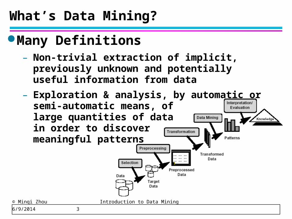
What’s Data Mining?

Many Definitions– Non-trivial extraction of implicit, previously

unknown and potentially useful information from data

– Exploration & analysis, by automatic or semi-automatic means, of large quantities of data in order to discover meaningful patterns


Data Mining Tasks

Prediction Methods– Use some variables to predict unknown or future

values of other variables.

Description Methods– Find human-interpretable patterns that describe the

data.

From [Fayyad, et.al.] Advances in Knowledge Discovery and Data Mining, 1996


Data Mining Tasks...

Classification [Predictive]

Clustering [Descriptive]

Association Rule Discovery [Descriptive]

Sequential Pattern Discovery [Descriptive]

Regression [Predictive]

Deviation Detection [Predictive]


Attribute Values

Attribute values are numbers or symbols assigned to an attribute

Distinction between attributes and attribute values– Same attribute can be mapped to different attribute

values Example: height can be measured in feet or meters

– Different attributes can be mapped to the same set of values Example: Attribute values for ID and age are integers But properties of attribute values can be different

– ID has no limit but age has a maximum and minimum value


Types of Attributes

There are different types of attributes– Nominal

Examples: ID numbers, eye color, zip codes

– Ordinal Examples: rankings (e.g., taste of potato chips on a scale

from 1-10), grades, height in {tall, medium, short}

– Interval Examples: calendar dates, temperatures in Celsius or

Fahrenheit.

– Ratio Examples: temperature in Kelvin, length, time, counts


Aggregation

Combining two or more attributes (or objects) into a single attribute (or object)

Purpose– Data reduction

Reduce the number of attributes or objects

– Change of scale Cities aggregated into regions, states, countries, etc

– More “stable” data Aggregated data tends to have less variability


Sampling …

The key principle for effective sampling is the following: – using a sample will work almost as well as using the

entire data sets, if the sample is representative

– A sample is representative if it has approximately the same property (of interest) as the original set of data


Dimensionality Reduction

Purpose:– Avoid curse of dimensionality– Reduce amount of time and memory required by data

mining algorithms– Allow data to be more easily visualized– May help to eliminate irrelevant features or reduce

noise

Techniques– Principle Component Analysis– Singular Value Decomposition– Others: supervised and non-linear techniques


Similarity and Dissimilarity

Similarity– Numerical measure of how alike two data objects are.

– Is higher when objects are more alike.

– Often falls in the range [0,1]

Dissimilarity– Numerical measure of how different are two data

objects

– Lower when objects are more alike

– Minimum dissimilarity is often 0

– Upper limit varies

Proximity refers to a similarity or dissimilarity


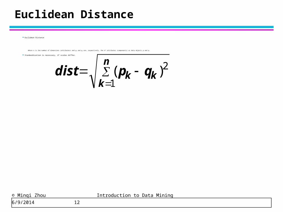
Euclidean Distance

Euclidean Distance

Where n is the number of dimensions (attributes) and pk and qk are, respectively, the kth attributes (components) or data objects p and q.

Standardization is necessary, if scales differ.

n

kkk qpdist

1

2)(


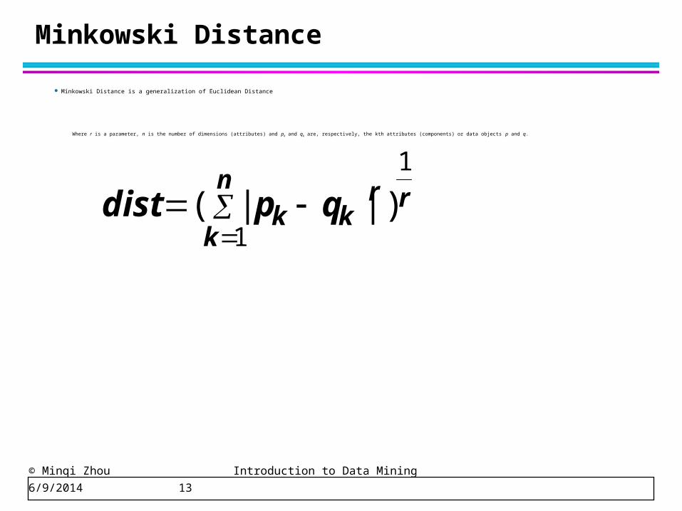
Minkowski Distance

Minkowski Distance is a generalization of Euclidean Distance

Where r is a parameter, n is the number of dimensions (attributes) and pk and qk are, respectively, the kth attributes (components) or data objects p and q.

rn

k

rkk qpdist

1

1)||(


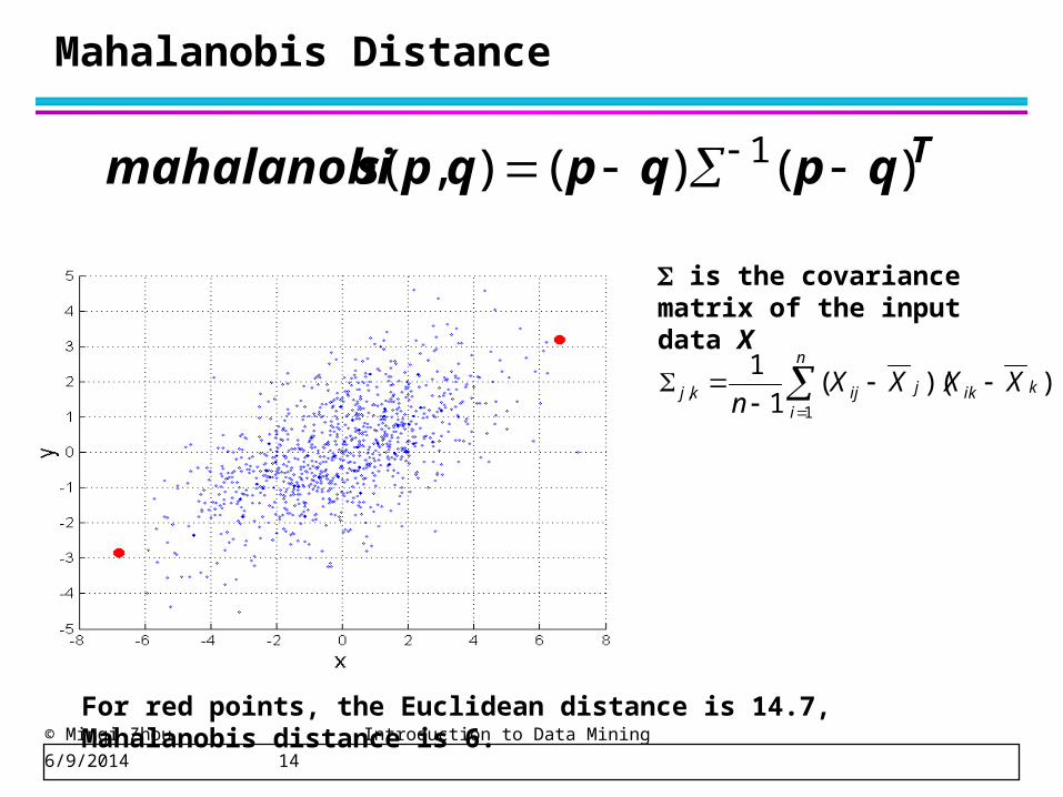
Mahalanobis Distance

Tqpqpqpsmahalanobi )()(),( 1

For red points, the Euclidean distance is 14.7, Mahalanobis distance is 6.

is the covariance matrix of the input data X

n

i

kikjijkj XXXXn 1

, ))((1

1


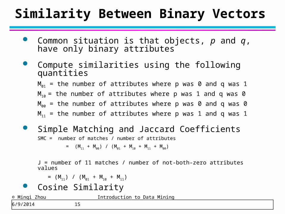
Similarity Between Binary Vectors

Common situation is that objects, p and q, have only binary attributes

Compute similarities using the following quantitiesM01 = the number of attributes where p was 0 and q was 1

M10 = the number of attributes where p was 1 and q was 0



Simple Matching and Jaccard Coefficients SMC = number of matches / number of attributes

= (M11 + M00) / (M01 + M10 + M11 + M00)

J = number of 11 matches / number of not-both-zero attributes values

= (M11) / (M01 + M10 + M11)

Cosine Similarity


Techniques Used In Data Exploration

In EDA, as originally defined by Tukey– The focus was on visualization

In our discussion of data exploration, we focus on– Summary statistics

Frequency: frequency, mode, percentialLocation: mean, medianSpread: range, variance,

– VisualizationHistogramBox plotScatter plotMatrix plot

– Online Analytical Processing (OLAP)


data exploration

Visualization– Parallel Coordination

– Star plot, chernoff face

OLAP– Multi-dimension array

– Data cubeSlice diceRoll-up, drill-down


Classification: Definition

Given a collection of records (training set )– Each record contains a set of attributes, one of the

attributes is the class. Find a model for class attribute as a function

of the values of other attributes. Goal: previously unseen records should be

assigned a class as accurately as possible.– A test set is used to determine the accuracy of the

model. Usually, the given data set is divided into training and test sets, with training set used to build the model and test set used to validate it.


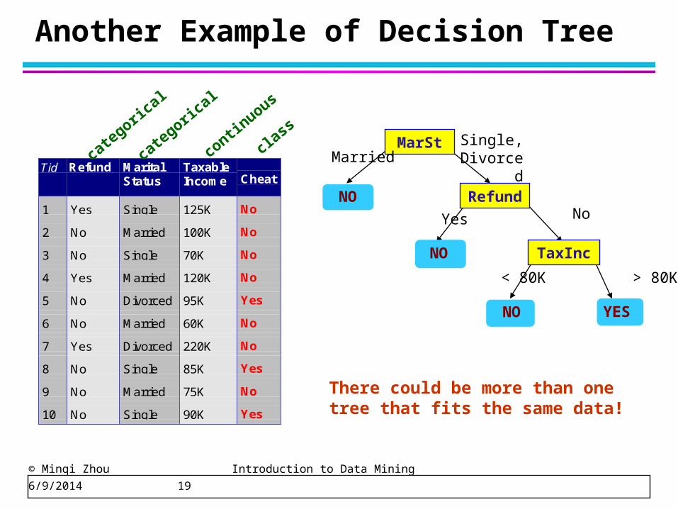
Another Example of Decision Tree

Tid Refund MaritalStatus

TaxableIncome Cheat

1 Yes Single 125K No

2 No Married 100K No

3 No Single 70K No

4 Yes Married 120K No

5 No Divorced 95K Yes

6 No Married 60K No

7 Yes Divorced 220K No

8 No Single 85K Yes

9 No Married 75K No

10 No Single 90K Yes10

categoric

al

categoric

al

continuous

classMarSt

Refund

TaxInc

YESNO

NO

NO

Yes No

Married Single,

Divorced

< 80K > 80K

There could be more than one tree that fits the same data!


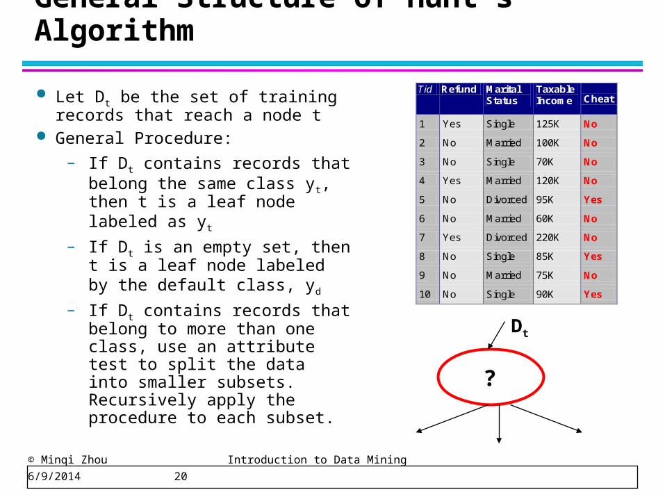
General Structure of Hunt’s Algorithm

Let Dt be the set of training records that reach a node t

General Procedure:

– If Dt contains records that belong the same class yt, then t is a leaf node labeled as yt

– If Dt is an empty set, then t is a leaf node labeled by the default class, yd

– If Dt contains records that belong to more than one class, use an attribute test to split the data into smaller subsets. Recursively apply the procedure to each subset.

Tid Refund Marital Status

Taxable Income Cheat

1 Yes Single 125K No

2 No Married 100K No

3 No Single 70K No

4 Yes Married 120K No

5 No Divorced 95K Yes

6 No Married 60K No

7 Yes Divorced 220K No

8 No Single 85K Yes

9 No Married 75K No

10 No Single 90K Yes 10

Dt

?


Tree Induction

Greedy strategy.– Split the records based on an attribute test that

optimizes certain criterion.

Issues– Determine how to split the records

How to specify the attribute test condition?How to determine the best split?

– Determine when to stop splitting


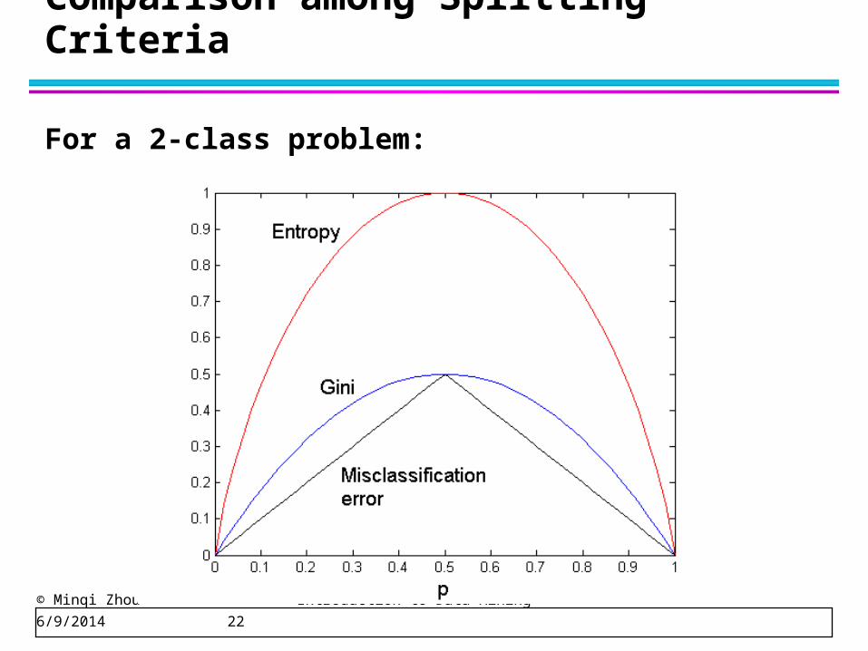
Comparison among Splitting Criteria

For a 2-class problem:


Practical Issues of Classification

Underfitting and Overfitting– Insufficient records, data noise

– Evaluation decision treesRe-substitution error, Generalization errorPre-pruning, post-pruning

Missing Values– In terms of the probability of visible data on class

Costs of Classification


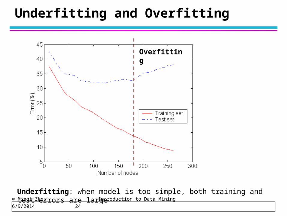
Underfitting and Overfitting

Overfitting

Underfitting: when model is too simple, both training and test errors are large


Occam’s Razor

Given two models of similar generalization errors, one should prefer the simpler model over the more complex model

For complex models, there is a greater chance that it was fitted accidentally by errors in data

Therefore, one should include model complexity when evaluating a model


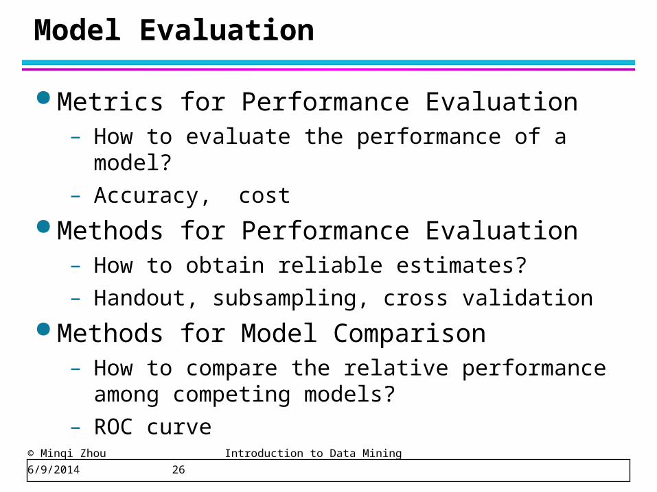
Model Evaluation

Metrics for Performance Evaluation– How to evaluate the performance of a model?

– Accuracy, cost

Methods for Performance Evaluation– How to obtain reliable estimates?

– Handout, subsampling, cross validation

Methods for Model Comparison– How to compare the relative performance among

competing models?

– ROC curve


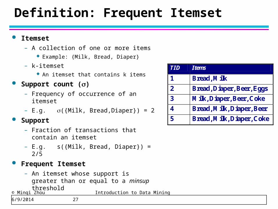
Definition: Frequent Itemset

Itemset– A collection of one or more items

Example: {Milk, Bread, Diaper}

– k-itemset An itemset that contains k items

Support count ()– Frequency of occurrence of an itemset

– E.g. ({Milk, Bread,Diaper}) = 2

Support– Fraction of transactions that contain an

itemset

– E.g. s({Milk, Bread, Diaper}) = 2/5

Frequent Itemset– An itemset whose support is greater

than or equal to a minsup threshold

TID Items

1 Bread, Milk

2 Bread, Diaper, Beer, Eggs

3 Milk, Diaper, Beer, Coke

4 Bread, Milk, Diaper, Beer

5 Bread, Milk, Diaper, Coke


Mining Association Rules

Two-step approach: 1. Frequent Itemset Generation

– Generate all itemsets whose support minsup

2. Rule Generation– Generate high confidence rules from each frequent itemset,

where each rule is a binary partitioning of a frequent itemset

Frequent itemset generation is still computationally expensive


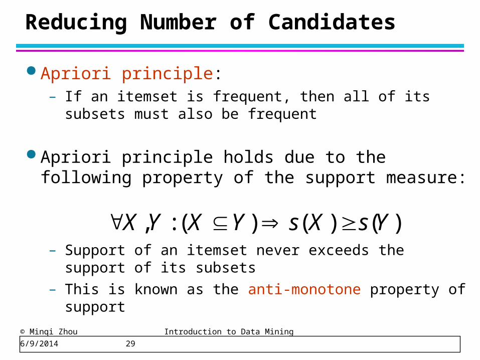
Reducing Number of Candidates

Apriori principle:– If an itemset is frequent, then all of its subsets must also

be frequent

Apriori principle holds due to the following property of the support measure:

– Support of an itemset never exceeds the support of its subsets

– This is known as the anti-monotone property of support

)()()(:, YsXsYXYX


Apriori Algorithm

Frequent itemset generation Frequent itemset support computation

– Brute-force

– Hash-tree

Rule generation– Rule generated under the same itemset


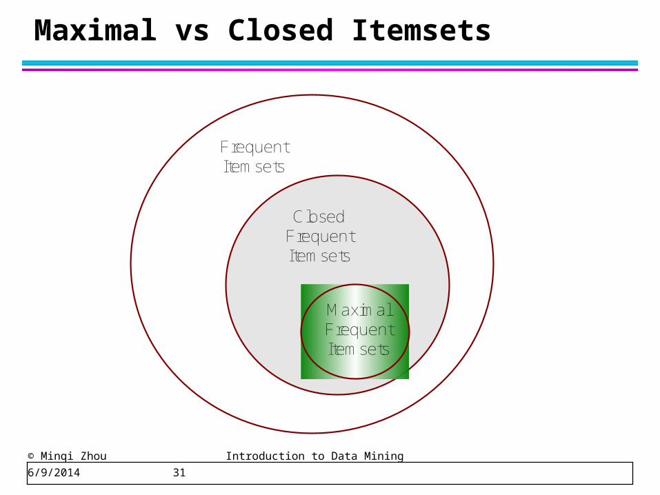
Maximal vs Closed Itemsets

FrequentItemsets

ClosedFrequentItemsets

MaximalFrequentItemsets


FP-growth Algorithm

Use a compressed representation of the database using an FP-tree

Once an FP-tree has been constructed, it uses a recursive divide-and-conquer approach to mine the frequent itemsets


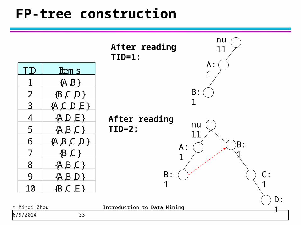
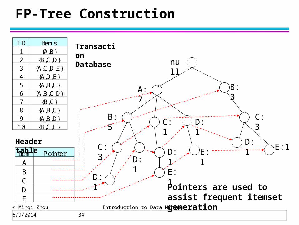
FP-tree construction

TID Items1 {A,B}2 {B,C,D}3 {A,C,D,E}4 {A,D,E}5 {A,B,C}6 {A,B,C,D}7 {B,C}8 {A,B,C}9 {A,B,D}10 {B,C,E}

null

A:1

B:1

null

A:1

B:1

B:1

C:1

D:1

After reading TID=1:

After reading TID=2:


FP-Tree Construction

null

A:7

B:5

B:3

C:3

D:1

C:1

D:1C:3

D:1

D:1

E:1E:1

TID Items1 {A,B}2 {B,C,D}3 {A,C,D,E}4 {A,D,E}5 {A,B,C}6 {A,B,C,D}7 {B,C}8 {A,B,C}9 {A,B,D}10 {B,C,E}

Pointers are used to assist frequent itemset generation

D:1

E:1

Transaction Database

Item PointerABCDE

Header table


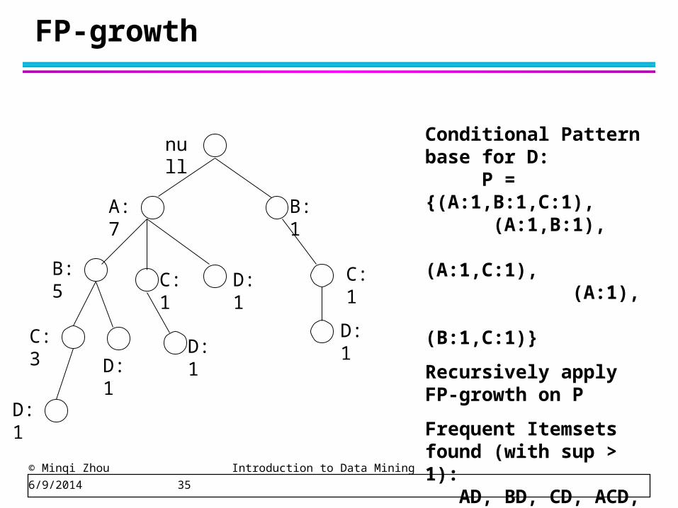
FP-growth

null

A:7

B:5

B:1

C:1

D:1

C:1

D:1C:3

D:1

D:1

Conditional Pattern base for D: P = {(A:1,B:1,C:1),

(A:1,B:1), (A:1,C:1), (A:1), (B:1,C:1)}

Recursively apply FP-growth on P

Frequent Itemsets found (with sup > 1): AD, BD, CD, ACD, BCD

D:1


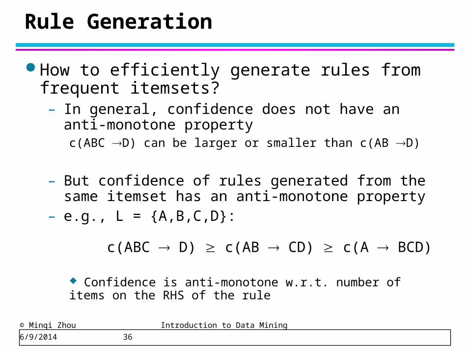
Rule Generation

How to efficiently generate rules from frequent itemsets?– In general, confidence does not have an anti-monotone

propertyc(ABC D) can be larger or smaller than c(AB

D)

– But confidence of rules generated from the same itemset has an anti-monotone property

– e.g., L = {A,B,C,D}:

c(ABC D) c(AB CD) c(A BCD) Confidence is anti-monotone w.r.t. number of items on the RHS of the rule


Types of Clusterings

A clustering is a set of clusters

Important distinction between hierarchical and partitional sets of clusters

Partitional Clustering– A division data objects into non-overlapping subsets (clusters)

such that each data object is in exactly one subset

Hierarchical clustering– A set of nested clusters organized as a hierarchical tree


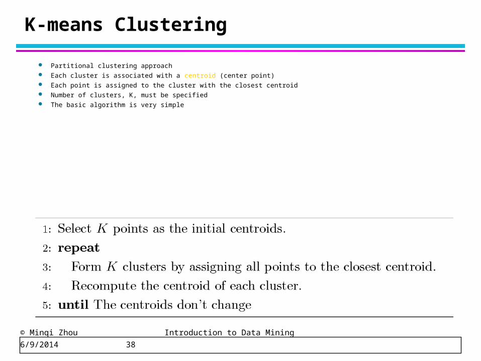
K-means Clustering

Partitional clustering approach Each cluster is associated with a centroid (center point) Each point is assigned to the cluster with the closest centroid Number of clusters, K, must be specified The basic algorithm is very simple


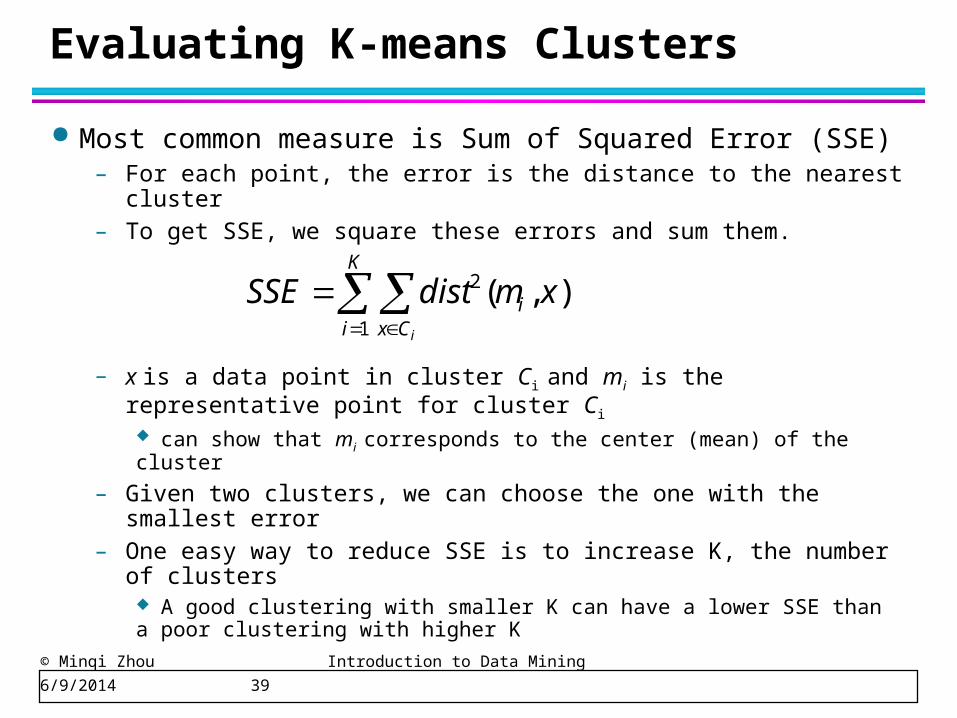
Evaluating K-means Clusters

Most common measure is Sum of Squared Error (SSE)– For each point, the error is the distance to the nearest cluster– To get SSE, we square these errors and sum them.

– x is a data point in cluster Ci and mi is the representative point for cluster Ci can show that mi corresponds to the center (mean) of the cluster

– Given two clusters, we can choose the one with the smallest error

– One easy way to reduce SSE is to increase K, the number of clusters A good clustering with smaller K can have a lower SSE than a poor clustering with higher K

K

i Cxi

i

xmdistSSE1

2 ),(


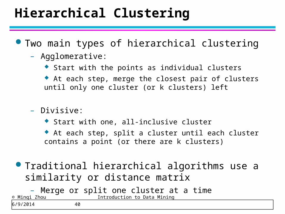
Hierarchical Clustering

Two main types of hierarchical clustering– Agglomerative:

Start with the points as individual clusters At each step, merge the closest pair of clusters until only one cluster (or k clusters) left

– Divisive: Start with one, all-inclusive cluster At each step, split a cluster until each cluster contains a point (or there are k clusters)

Traditional hierarchical algorithms use a similarity or distance matrix

– Merge or split one cluster at a time


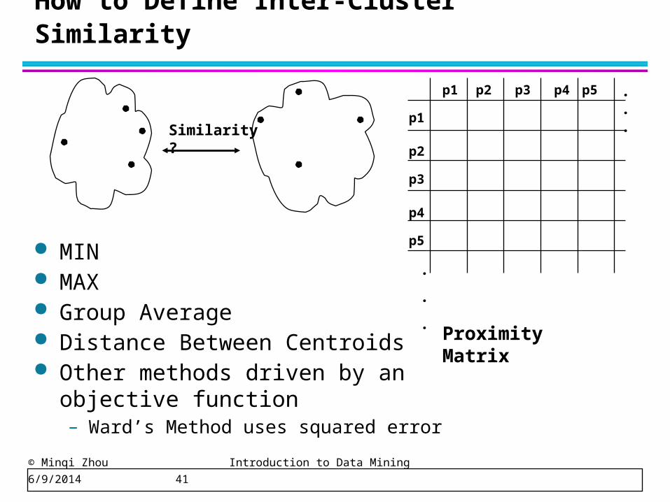
How to Define Inter-Cluster Similarity

p1

p3

p5

p4

p2

p1 p2 p3 p4 p5 . . .

.

.

.

Similarity?

MIN MAX Group Average Distance Between Centroids Other methods driven by an objective

function– Ward’s Method uses squared error

Proximity Matrix


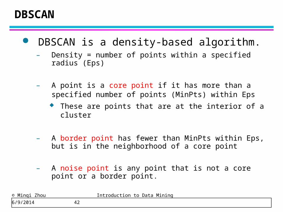
DBSCAN

DBSCAN is a density-based algorithm.– Density = number of points within a specified radius (Eps)

– A point is a core point if it has more than a specified number of points (MinPts) within Eps

These are points that are at the interior of a cluster

– A border point has fewer than MinPts within Eps, but is in the neighborhood of a core point

– A noise point is any point that is not a core point or a border point.


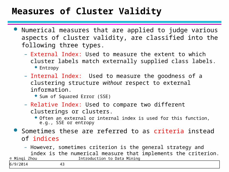
Numerical measures that are applied to judge various aspects of cluster validity, are classified into the following three types.– External Index: Used to measure the extent to which cluster labels

match externally supplied class labels. Entropy

– Internal Index: Used to measure the goodness of a clustering structure without respect to external information.

Sum of Squared Error (SSE)

– Relative Index: Used to compare two different clusterings or clusters.

Often an external or internal index is used for this function, e.g., SSE or entropy

Sometimes these are referred to as criteria instead of indices– However, sometimes criterion is the general strategy and index is the

numerical measure that implements the criterion.

Measures of Cluster Validity


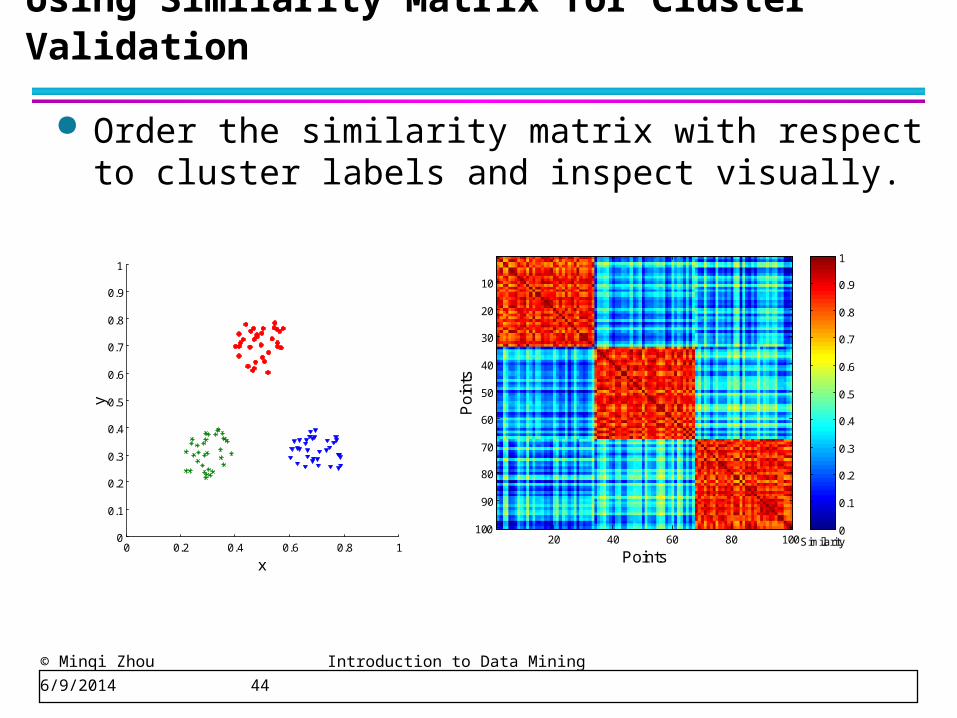
Order the similarity matrix with respect to cluster labels and inspect visually.

Using Similarity Matrix for Cluster Validation

0 0.2 0.4 0.6 0.8 10

0.1

0.2

0.3

0.4

0.5

0.6

0.7

0.8

0.9

1

x

y

Points

Po

ints

20 40 60 80 100

10

20

30

40

50

60

70

80

90

100Similarity

0

0.1

0.2

0.3

0.4

0.5

0.6

0.7

0.8

0.9

1

Documents

Data Mining Go Over Lecture Notes for Go Over Introduction to Data Mining by Minqi Zhou © Tan,Steinbach, Kumar Introduction to Data Mining 4/18/2004 1