Embed Size (px)
Citation preview

Data Mining:Unsupervised Learning
Business Analytics PracticeWinter Term 2015/16
Stefan Feuerriegel
Today’s Lecture
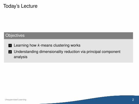
Objectives
1 Learning how k -means clustering works
2 Understanding dimensionality reduction via principal componentanalysis
2Unsupervised Learning
Outline
1 Motivation
2 k -Means Clustering
3 Principal Component Analysis
4 Wrap-Up
3Unsupervised Learning
Outline
1 Motivation
2 k -Means Clustering
3 Principal Component Analysis
4 Wrap-Up
4Unsupervised Learning: Motivation
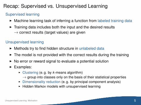
Recap: Supervised vs. Unsupervised Learning
Supervised learning
I Machine learning task of inferring a function from labeled training data
I Training data includes both the input and the desired results→ correct results (target values) are given
Unsupervised learning
I Methods try to find hidden structure in unlabeled data
I The model is not provided with the correct results during the training
I No error or reward signal to evaluate a potential solutionI Examples:
I Clustering (e. g. by k -means algorithm)→ group into classes only on the basis of their statistical properties
I Dimensionality reduction (e. g. by principal component analysis)I Hidden Markov models with unsupervised learning
5Unsupervised Learning: Motivation
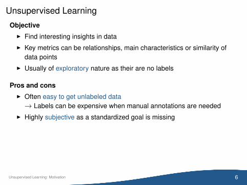
Unsupervised Learning
ObjectiveI Find interesting insights in data
I Key metrics can be relationships, main characteristics or similarity ofdata points
I Usually of exploratory nature as their are no labels
Pros and consI Often easy to get unlabeled data→ Labels can be expensive when manual annotations are needed
I Highly subjective as a standardized goal is missing
6Unsupervised Learning: Motivation
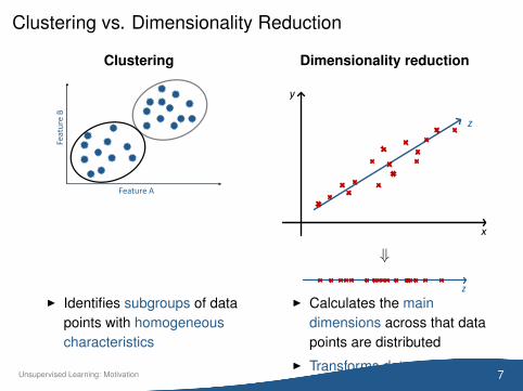
Clustering vs. Dimensionality Reduction
Clustering
Feature A
Feat
ure
BDimensionality reduction
y
x
z
⇓
z
I Identifies subgroups of datapoints with homogeneouscharacteristics
I Calculates the maindimensions across that datapoints are distributed
I Transforms data onto thatsubset of dimensions
7Unsupervised Learning: Motivation
Outline
1 Motivation
2 k -Means Clustering
3 Principal Component Analysis
4 Wrap-Up
8Unsupervised Learning: k -Means Clustering
k -Means Clustering
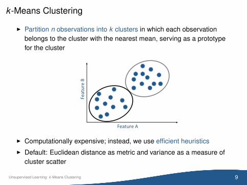
I Partition n observations into k clusters in which each observationbelongs to the cluster with the nearest mean, serving as a prototypefor the cluster
Feature A
Feat
ure
B
I Computationally expensive; instead, we use efficient heuristics
I Default: Euclidean distance as metric and variance as a measure ofcluster scatter
9Unsupervised Learning: k -Means Clustering
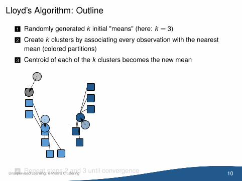
Lloyd’s Algorithm: Outline
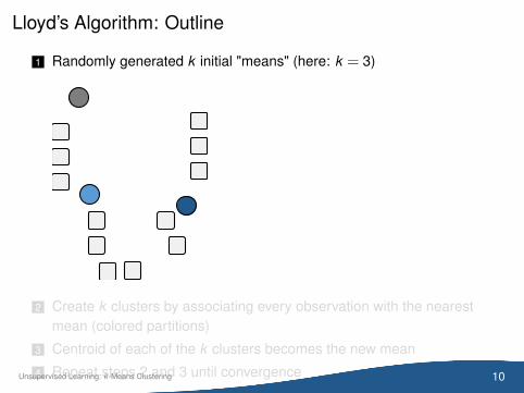
1 Randomly generated k initial "means" (here: k = 3)
2 Create k clusters by associating every observation with the nearestmean (colored partitions)
3 Centroid of each of the k clusters becomes the new mean
4 Repeat steps 2 and 3 until convergence 10Unsupervised Learning: k -Means Clustering
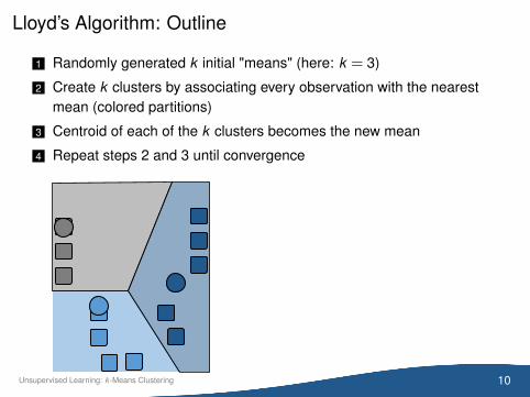
Lloyd’s Algorithm: Outline
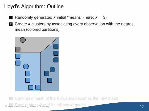
1 Randomly generated k initial "means" (here: k = 3)
2 Create k clusters by associating every observation with the nearestmean (colored partitions)
3 Centroid of each of the k clusters becomes the new mean
4 Repeat steps 2 and 3 until convergence 10Unsupervised Learning: k -Means Clustering
Lloyd’s Algorithm: Outline
1 Randomly generated k initial "means" (here: k = 3)
2 Create k clusters by associating every observation with the nearestmean (colored partitions)
3 Centroid of each of the k clusters becomes the new mean
4 Repeat steps 2 and 3 until convergence
10Unsupervised Learning: k -Means Clustering
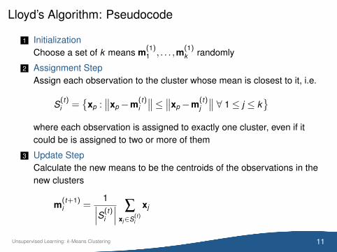
Lloyd’s Algorithm: Pseudocode
1 InitializationChoose a set of k means m(1)
1 , . . . ,m(1)k randomly
2 Assignment StepAssign each observation to the cluster whose mean is closest to it, i.e.
S(t)i =
{xp :
∥∥xp−m(t)i
∥∥≤ ∥∥xp−m(t)j
∥∥ ∀ 1≤ j ≤ k}
where each observation is assigned to exactly one cluster, even if itcould be is assigned to two or more of them
3 Update StepCalculate the new means to be the centroids of the observations in thenew clusters
m(t+1)i =
1∣∣∣S(t)i
∣∣∣ ∑xj∈S(t)
i
xj
11Unsupervised Learning: k -Means Clustering
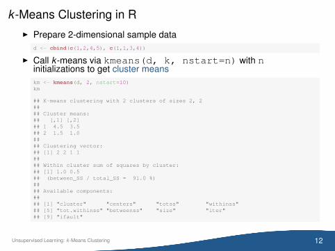
k -Means Clustering in RI Prepare 2-dimensional sample data
d <- cbind(c(1,2,4,5), c(1,1,3,4))
I Call k -means via kmeans(d, k, nstart=n) with ninitializations to get cluster meanskm <- kmeans(d, 2, nstart=10)km
## K-means clustering with 2 clusters of sizes 2, 2#### Cluster means:## [,1] [,2]## 1 4.5 3.5## 2 1.5 1.0#### Clustering vector:## [1] 2 2 1 1#### Within cluster sum of squares by cluster:## [1] 1.0 0.5## (between_SS / total_SS = 91.0 %)#### Available components:#### [1] "cluster" "centers" "totss" "withinss"## [5] "tot.withinss" "betweenss" "size" "iter"## [9] "ifault"
12Unsupervised Learning: k -Means Clustering
k -Means Clustering in R
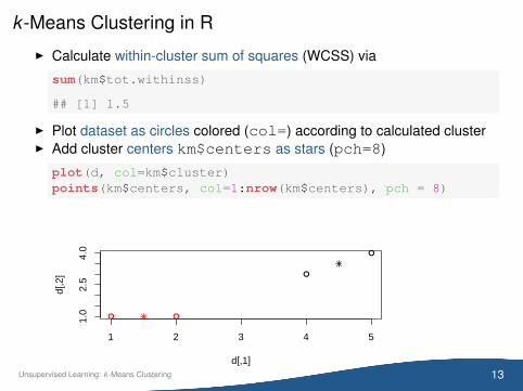
I Calculate within-cluster sum of squares (WCSS) via
sum(km$tot.withinss)
## [1] 1.5
I Plot dataset as circles colored (col=) according to calculated clusterI Add cluster centers km$centers as stars (pch=8)
plot(d, col=km$cluster)points(km$centers, col=1:nrow(km$centers), pch = 8)
● ●
●
●
1 2 3 4 5
1.0
2.5
4.0
d[,1]
d[,2
]
13Unsupervised Learning: k -Means Clustering
Optimal Choice of k
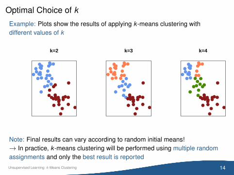
Example: Plots show the results of applying k -means clustering withdifferent values of k
●
●
●
●
●●
●
●
●
●
●●
●
●
●
●
●
● ●●
● ●
●●
●●
●●
●●
●
●●
● ●●
●
●
●●
●
●
●
●
●●
●
●
●
●
k=2
●
●
●
●
●●
●
●
●
●
●●
●
●
●
●
●
● ●●
● ●
●●
●●
●●
●●
●
●●
● ●●
●
●
●●
●
●
●
●
●●
●
●
●
●
k=3
●
●
●
●
●●
●
●
●
●
●●
●
●
●
●
●
● ●●
● ●
●●
●●
●●
●●
●
●●
● ●●
●
●
●●
●
●
●
●
●●
●
●
●
●
k=4
Note: Final results can vary according to random initial means!→ In practice, k -means clustering will be performed using multiple randomassignments and only the best result is reported
14Unsupervised Learning: k -Means Clustering
Optimal Choice of k
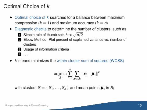
I Optimal choice of k searches for a balance between maximumcompression (k = 1) and maximum accuracy (k = n)
I Diagnostic checks to determine the number of clusters, such as1 Simple rule of thumb sets k ≈
√n/2
2 Elbow Method: Plot percent of explained variance vs. number ofclusters
3 Usage of information criteria4 . . .
I k -means minimizes the within-cluster sum of squares (WCSS)
argminS
k
∑i=1
∑xj∈Si
‖xj −µµµ i‖2
with clusters S = {S1, . . . ,Sk } and mean points µµµ i in Si
15Unsupervised Learning: k -Means Clustering

Clustering
Research Question
Group countries based on income, literacy, infant mortality and lifeexpectancy (file: countries.csv) into three groups accounting fordeveloped, emerging and undeveloped countries.
# Use first column as row names for each observationcountries <- read.csv("countries.csv", header=TRUE, sep=",", row.names=1)head(countries)
## Per.capita.income Literacy Infant.mortality Life.expectancy## Brazil 10326 90.0 23.60 75.4## Germany 39650 99.0 4.08 79.4## Mozambique 830 38.7 95.90 42.1## Australia 43163 99.0 4.57 81.2## China 5300 90.9 23.00 73.0## Argentina 13308 97.2 13.40 75.3
16Unsupervised Learning: k -Means Clustering
Clustering
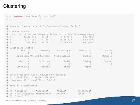
km <- kmeans(countries, 3, nstart=10)km
## K-means clustering with 3 clusters of sizes 7, 7, 5#### Cluster means:## Per.capita.income Literacy Infant.mortality Life.expectancy## 1 35642.143 98.50 4.477143 80.42857## 2 3267.286 70.50 56.251429 58.80000## 3 13370.400 91.58 23.560000 68.96000#### Clustering vector:## Brazil Germany Mozambique Australia China## 3 1 2 1 2## Argentina United Kingdom South Africa Zambia Namibia## 3 1 3 2 2## Georgia Pakistan India Turkey Sweden## 2 2 2 3 1## Lithuania Greece Italy Japan## 3 1 1 1#### Within cluster sum of squares by cluster:## [1] 158883600 20109876 57626083## (between_SS / total_SS = 94.1 %)#### Available components:#### [1] "cluster" "centers" "totss" "withinss"## [5] "tot.withinss" "betweenss" "size" "iter"## [9] "ifault"
17Unsupervised Learning: k -Means Clustering
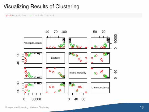
Visualizing Results of Clusteringplot(countries, col = km$cluster)
Per.capita.income
40 70 100
●
●
●
●
●●
●
●● ● ●● ●
●
●
●
●●●
●
●
●
●
●●
●
●●●● ●●
●
●
●
●●●
50 70
040
000
●
●
●
●
●●
●
●● ● ●●●
●
●
●
●●●
4090 ●
●
●
●●
● ●
●●
●●
●●
●●● ●● ●
Literacy●
●
●
●●
●●
●●
●●
●●
●●●●●● ●
●
●
●●●●
●●
●●
●●
●●● ●●●
●●
●
●●
● ●
●
●
●
●
●●
●
●● ●● ●●
●
●
●●
●●
●
●
●
●
●●
●
●●●●●
Infant.mortality
060
●●
●
●●●●
●
●
●
●
●●
●
●● ●●●
0 30000
5080 ● ●
●
●● ●
●
●●
●
●●●
●●
●●● ●
● ●
●
●●●
●
●●
●
●● ●
●●●
●●●
0 40 80
●●
●
●●●
●
●●
●
●●●
●●●●●●
Life.expectancy
18Unsupervised Learning: k -Means Clustering
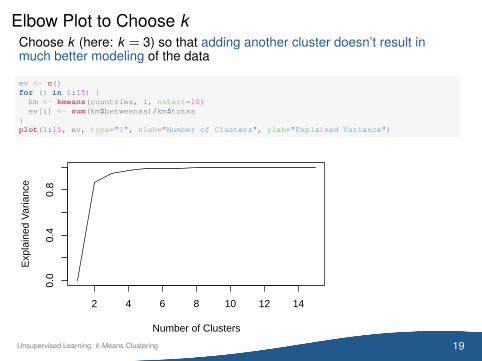
Elbow Plot to Choose kChoose k (here: k = 3) so that adding another cluster doesn’t result inmuch better modeling of the data
ev <- c()for (i in 1:15) {
km <- kmeans(countries, i, nstart=10)ev[i] <- sum(km$betweenss)/km$totss
}plot(1:15, ev, type="l", xlab="Number of Clusters", ylab="Explained Variance")
2 4 6 8 10 12 14
0.0
0.4
0.8
Number of Clusters
Exp
lain
ed V
aria
nce
19Unsupervised Learning: k -Means Clustering
Outline
1 Motivation
2 k -Means Clustering
3 Principal Component Analysis
4 Wrap-Up
20Unsupervised Learning: Principal Component Analysis
Principal Component Analysis
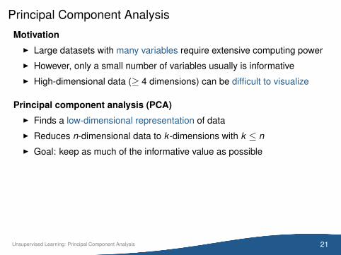
MotivationI Large datasets with many variables require extensive computing power
I However, only a small number of variables usually is informative
I High-dimensional data (≥ 4 dimensions) can be difficult to visualize
Principal component analysis (PCA)I Finds a low-dimensional representation of data
I Reduces n-dimensional data to k -dimensions with k ≤ n
I Goal: keep as much of the informative value as possible
21Unsupervised Learning: Principal Component Analysis
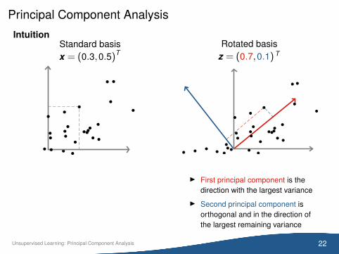
Principal Component Analysis
IntuitionStandard basisx = (0.3,0.5)T
Rotated basisz = (0.7,0.1) T
I First principal component is thedirection with the largest variance
I Second principal component isorthogonal and in the direction ofthe largest remaining variance
22Unsupervised Learning: Principal Component Analysis
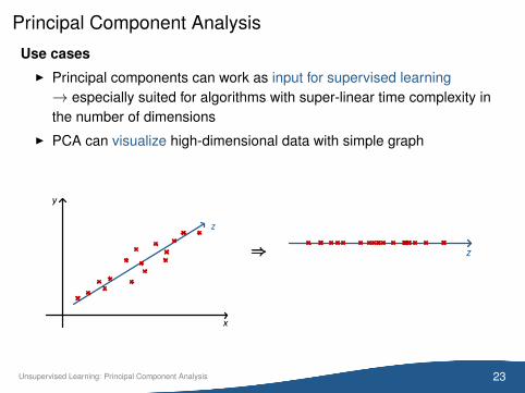
Principal Component Analysis
Use casesI Principal components can work as input for supervised learning→ especially suited for algorithms with super-linear time complexity inthe number of dimensions
I PCA can visualize high-dimensional data with simple graph
y
x
z
⇒⇒⇒ z
23Unsupervised Learning: Principal Component Analysis
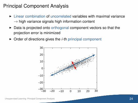
Principal Component Analysis
I Linear combination of uncorrelated variables with maximal variance→ high variance signals high information content
I Data is projected onto orthogonal component vectors so that theprojection error is minimized
I Order of directions gives the i-th principal component
30
–3030
20
10
0
–30 20100
–20
–20 –10
–10
24Unsupervised Learning: Principal Component Analysis
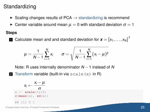
Standardizing
I Scaling changes results of PCA→ standardizing is recommend
I Center variable around mean µ = 0 with standard deviation σ = 1
Steps
1 Calculate mean and and standard deviation for x = [x1, . . . ,xN ]T
µ =1
N−1
N
∑i=1
xi σ =
√1
N−1
N
∑i=1
(xi −µ)2
Note: R uses internally denominator N−1 instead of N
2 Transform variable (built-in via scale(x) in R)
xi ←xi −µ
σx <- scale(1:10)c(mean(x), sd(x))
## [1] 0 1
25Unsupervised Learning: Principal Component Analysis
Algorithm
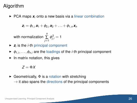
I PCA maps xi onto a new basis via a linear combination
zi = φ1,i x1 + φ2,i x2 + . . .+ φ1,n xn
with normalizationn∑
j=1φ 2
j,i = 1
I zi is the i-th principal component
I φ1,i , . . . ,φn,i are the loadings of the i-th principal component
I In matrix notation, this gives
Z = ΦX
I Geometrically, Φ is a rotation with stretching→ it also spans the directions of the principal components
26Unsupervised Learning: Principal Component Analysis
Algorithm
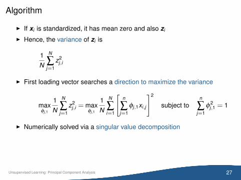
I If xi is standardized, it has mean zero and also zi
I Hence, the variance of zi is
1N
N
∑j=1
z2j,i
I First loading vector searches a direction to maximize the variance
maxφj,1
1N
N
∑j=1
z2j,i = max
φj,1
1N
N
∑i=1
[n
∑j=1
φj,1xi,j
]2
subject ton
∑j=1
φ2j,1 = 1
I Numerically solved via a singular value decomposition
27Unsupervised Learning: Principal Component Analysis
Singular Value Decomposition
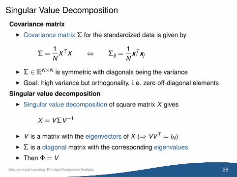
Covariance matrixI Covariance matrix Σ for the standardized data is given by
Σ =1N
X T X ⇔ Σij =1N
xTi xj
I Σ ∈ RN×N is symmetric with diagonals being the variance
I Goal: high variance but orthogonality, i. e. zero off-diagonal elements
Singular value decompositionI Singular value decomposition of square matrix X gives
X = VΣV−1
I V is a matrix with the eigenvectors of X (⇒ VV T = IN )
I Σ is a diagonal matrix with the corresponding eigenvalues
I Then Φ = V
28Unsupervised Learning: Principal Component Analysis
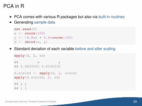
PCA in R
I PCA comes with various R packages but also via built-in routinesI Generating sample data
set.seed(0)x <- rnorm(100)y <- -0.8*x + 0.6*rnorm(100)d <- cbind(x, y)
I Standard deviation of each variable before and after scaling
apply(d, 2, sd)
## x y## 0.8826502 0.8546230
d.scaled <- apply(d, 2, scale)apply(d.scaled, 2, sd)
## x y## 1 1
29Unsupervised Learning: Principal Component Analysis
PCA in R
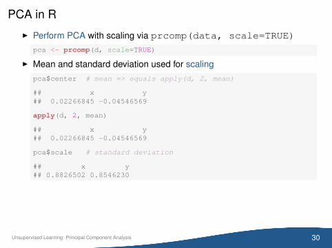
I Perform PCA with scaling via prcomp(data, scale=TRUE)
pca <- prcomp(d, scale=TRUE)
I Mean and standard deviation used for scalingpca$center # mean => equals apply(d, 2, mean)
## x y## 0.02266845 -0.04546569
apply(d, 2, mean)
## x y## 0.02266845 -0.04546569
pca$scale # standard deviation
## x y## 0.8826502 0.8546230
30Unsupervised Learning: Principal Component Analysis
PCA in R
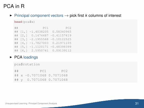
I Principal component vectors→ pick first k columns of interesthead(pca$x)
## PC1 PC2## [1,] -1.4038205 0.58340965## [2,] 0.1474487 -0.41157419## [3,] -2.1955568 -0.10122525## [4,] -1.7827003 0.21971105## [5,] -1.1120171 -0.48398399## [6,] 2.5950741 0.09139112
I PCA loadings
pca$rotation
## PC1 PC2## x -0.7071068 0.7071068## y 0.7071068 0.7071068
31Unsupervised Learning: Principal Component Analysis
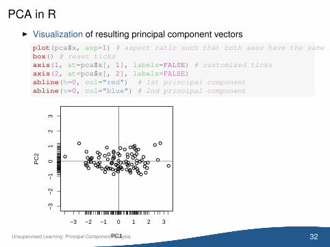
PCA in RI Visualization of resulting principal component vectors
plot(pca$x, asp=1) # aspect ratio such that both axes have the same scalebox() # reset ticksaxis(1, at=pca$x[, 1], labels=FALSE) # customized ticksaxis(2, at=pca$x[, 2], labels=FALSE)abline(h=0, col="red") # 1st principal componentabline(v=0, col="blue") # 2nd principal component
●
●
●
●
●
●
●
●
●
●
●
●
●●
●
●
●
●●
●●●
●●
●
●●
●
●
●
●
●
●
●
●
●● ●
●●
●
●
●
● ●●
●
●
●
●
●
●
●
●
●
●●
●
●●
●
●
●
●
●●
●
●
●
●
●
●●●●
●
●
●
●
●
●●●
●●
●
●
●
●
●
●●
●
●
●
●
●
●
●●
−3 −2 −1 0 1 2 3
−3
−2
−1
01
23
PC1
PC
2
32Unsupervised Learning: Principal Component Analysis
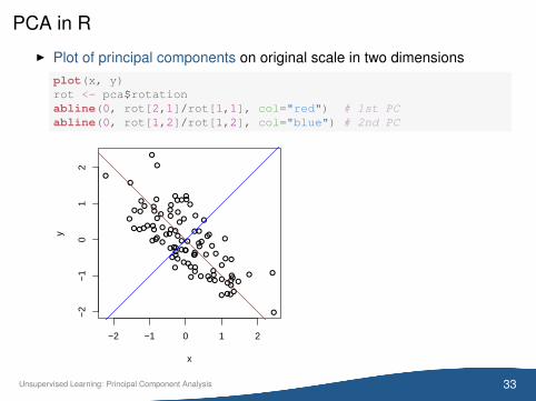
PCA in R
I Plot of principal components on original scale in two dimensionsplot(x, y)rot <- pca$rotationabline(0, rot[2,1]/rot[1,1], col="red") # 1st PCabline(0, rot[1,2]/rot[1,2], col="blue") # 2nd PC
●
●
●
●●
●
●
●
●
●●
●
●
●
●
●
●
●
●
●
●
●
●
●
●
●
●
●
●
●
●
●
●
●●
●●
●
●
●
●
●
●●
●●●
●
●●
●
●
●
●
●
●
●
●
●
●
●●
●
●●
●
●
●
●
●
●
●
●
●
●
●
●
●
●●
●
●
●
●●
●
●
●
●
●
●
●
●
●●
●
●
●
●
●
−2 −1 0 1 2
−2
−1
01
2
x
y
33Unsupervised Learning: Principal Component Analysis
PCA in R
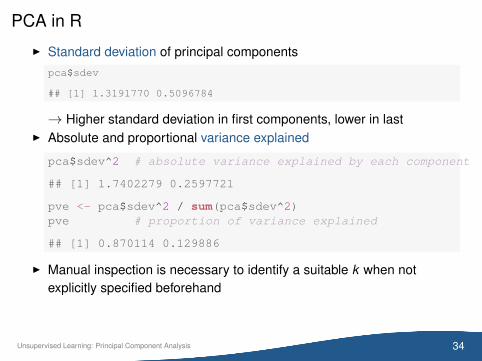
I Standard deviation of principal componentspca$sdev
## [1] 1.3191770 0.5096784
→ Higher standard deviation in first components, lower in lastI Absolute and proportional variance explained
pca$sdev^2 # absolute variance explained by each component
## [1] 1.7402279 0.2597721
pve <- pca$sdev^2 / sum(pca$sdev^2)pve # proportion of variance explained
## [1] 0.870114 0.129886
I Manual inspection is necessary to identify a suitable k when notexplicitly specified beforehand
34Unsupervised Learning: Principal Component Analysis
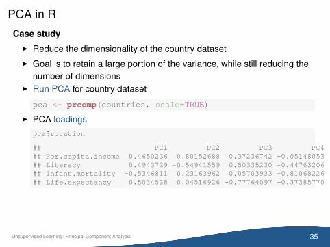
PCA in R
Case studyI Reduce the dimensionality of the country dataset
I Goal is to retain a large portion of the variance, while still reducing thenumber of dimensions
I Run PCA for country dataset
pca <- prcomp(countries, scale=TRUE)
I PCA loadingspca$rotation
## PC1 PC2 PC3 PC4## Per.capita.income 0.4650236 0.80152688 0.37236742 -0.05148053## Literacy 0.4943729 -0.54941559 0.50335230 -0.44763206## Infant.mortality -0.5346811 0.23163962 0.05703933 -0.81068226## Life.expectancy 0.5034528 0.04516926 -0.77764097 -0.37385770
35Unsupervised Learning: Principal Component Analysis
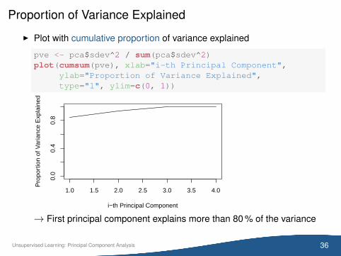
Proportion of Variance Explained
I Plot with cumulative proportion of variance explained
pve <- pca$sdev^2 / sum(pca$sdev^2)plot(cumsum(pve), xlab="i-th Principal Component",
ylab="Proportion of Variance Explained",type="l", ylim=c(0, 1))
1.0 1.5 2.0 2.5 3.0 3.5 4.0
0.0
0.4
0.8
i−th Principal Component
Pro
port
ion
of V
aria
nce
Exp
lain
ed
→ First principal component explains more than 80 % of the variance
36Unsupervised Learning: Principal Component Analysis
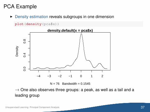
PCA Example
I Density estimation reveals subgroups in one dimension
plot(density(pca$x))
−4 −3 −2 −1 0 1 2
0.0
0.4
0.8
density.default(x = pca$x)
N = 76 Bandwidth = 0.1545
Den
sity
→ One also observes three groups: a peak, as well as a tail and aleading group
37Unsupervised Learning: Principal Component Analysis
Outline
1 Motivation
2 k -Means Clustering
3 Principal Component Analysis
4 Wrap-Up
38Unsupervised Learning: Wrap-Up
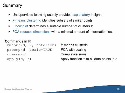
Summary
I Unsupervised learning usually provides explanatory insights
I k -means clustering identifies subsets of similar points
I Elbow plot determines a suitable number of clusters k
I PCA reduces dimensions with a minimal amount of information loss
Commands in Rkmeans(d, k, nstart=n) k -means clusterinprcomp(d, scale=TRUE) PCA with scalingcumsum(x) Cumulative sumsapply(d, f) Apply function f to all data points in d
39Unsupervised Learning: Wrap-Up