Data Mining Using Matlab

University of Southern Queensland

Faculty of Engineering & Surveying

Data Mining Using Matlab

A dissertation submitted by

Rodney J. Woolf

in fulfilment of the requirements of

ENG4112 Research Project

towards the degree of

Bachelor of Engineering (Mechatronics)

Submitted: January, 2005

ii

Abstract

Data mining is a relatively new field emerging in many disciplines. It is becoming more

popular as technology advances, and the need for efficient data analysis is required.

The aim of data mining itself is not to provide strict rules by analysing the full data

set, data mining is used to predict with some certainty while only analysing a small

portion of the data. This project seeks to compare the efficiency of a decision tree

induction method with that of the neural network method.

MATLAB has inbuilt data mining toolboxes. However the decision tree induction

method is not as yet implemented. Decision tree induction has been implemented in

several forms in the past. The greatest contribution to this method has been made by

DR John Ross Quinlan, who has brought forward this method in the form of ID3, C4.5

and C5 algorithms. The methodologies used within ID3 and C4.5 are well documented

and therefore provide a strong platform for the implementation of this method within

a higher level language.

The objectives of this study are to fully comprehend two methods of data mining,

namely decision tree induction and neural networks. The decision tree induction

method is to be implemented within the mathematical computer language MATLAB.

The results found when analysing some suitable data will be compared with the results

from the neural network toolbox already implemented in MATLAB.

The data used to compare and contrast the two methods included voting records from

the US House of Representatives, which consists of yes, no and undecided votes on six-

teen separate issues. The voters are grouped into categories according to their political

party. This can be either republican or democratic. The objective of using this data

set is to predict what party a congressman is affiliated with by analysing their voting

trends.

The findings of this study reveal that the decision tree method can accurately predict

outcomes if an ideal data set is used for building the tree. The neural network method

has less accuracy in some situations however it is more robust towards unexpected data.


Faculty of Engineering and Surveying

ENG4111/2 Research Project

Limitations of Use

The Council of the University of Southern Queensland, its Faculty of Engineering and

Surveying, and the staff of the University of Southern Queensland, do not accept any

responsibility for the truth, accuracy or completeness of material contained within or

associated with this dissertation.

Persons using all or any part of this material do so at their own risk, and not at the

risk of the Council of the University of Southern Queensland, its Faculty of Engineering

and Surveying or the staff of the University of Southern Queensland.

This dissertation reports an educational exercise and has no purpose or validity beyond

this exercise. The sole purpose of the course pair entitled “Research Project” is to

contribute to the overall education within the student’s chosen degree program. This

document, the associated hardware, software, drawings, and other material set out in

the associated appendices should not be used for any other purpose: if they are so used,

it is entirely at the risk of the user.

Prof G Baker

Dean


Certification of Dissertation

I certify that the ideas, designs and experimental work, results, analyses and conclusions

set out in this dissertation are entirely my own effort, except where otherwise indicated

and acknowledged.

I further certify that the work is original and has not been previously submitted for

assessment in any other course or institution, except where specifically stated.

Rodney J. Woolf

Q10222583

Signature

Date

Contents

List of Figures x

List of Tables xi

Chapter 1 Introduction 1

1.1 Introduction . . . . . . . . . . . . . . . . . . . . . . . . . . . . . . . . . . 1

1.2 Background . . . . . . . . . . . . . . . . . . . . . . . . . . . . . . . . . . 1

1.3 Objectives . . . . . . . . . . . . . . . . . . . . . . . . . . . . . . . . . . . 2

1.4 Scope . . . . . . . . . . . . . . . . . . . . . . . . . . . . . . . . . . . . . 2

Chapter 2 Literature Review 4

2.1 Data mining applications in engineering . . . . . . . . . . . . . . . . . . 4

2.2 Machine Learning . . . . . . . . . . . . . . . . . . . . . . . . . . . . . . . 5

2.2.1 Introduction . . . . . . . . . . . . . . . . . . . . . . . . . . . . . 5

2.2.2 Decision Tree Learning . . . . . . . . . . . . . . . . . . . . . . . . 5

2.2.3 ID3 . . . . . . . . . . . . . . . . . . . . . . . . . . . . . . . . . . 6

CONTENTS vi

2.2.4 Entropy . . . . . . . . . . . . . . . . . . . . . . . . . . . . . . . . 8

2.2.5 Noise . . . . . . . . . . . . . . . . . . . . . . . . . . . . . . . . . 8

2.2.6 C4.5 . . . . . . . . . . . . . . . . . . . . . . . . . . . . . . . . . . 9

2.2.7 Missing Values . . . . . . . . . . . . . . . . . . . . . . . . . . . . 10

2.2.8 Continuous Data . . . . . . . . . . . . . . . . . . . . . . . . . . . 10

2.2.9 Discretization techniques . . . . . . . . . . . . . . . . . . . . . . 10

2.3 Artificial Neural Networks . . . . . . . . . . . . . . . . . . . . . . . . . . 12

2.3.1 Backpropagation . . . . . . . . . . . . . . . . . . . . . . . . . . . 14

2.3.2 Multilayer Networks . . . . . . . . . . . . . . . . . . . . . . . . . 15

2.3.3 Training Neural Networks . . . . . . . . . . . . . . . . . . . . . . 15

2.3.4 Applications of Neural Netwoks . . . . . . . . . . . . . . . . . . . 16

Chapter 3 Methodology 17

3.1 Program Methodology . . . . . . . . . . . . . . . . . . . . . . . . . . . . 17

3.2 Decision Tree Induction . . . . . . . . . . . . . . . . . . . . . . . . . . . 17

3.3 Program Modules . . . . . . . . . . . . . . . . . . . . . . . . . . . . . . . 18

3.3.1 Data Input Methods/Data Structure . . . . . . . . . . . . . . . . 18

3.3.2 Data Output Method/Structure . . . . . . . . . . . . . . . . . . 22

3.3.3 Continuous Data . . . . . . . . . . . . . . . . . . . . . . . . . . . 25

3.3.4 Rule Contradictions . . . . . . . . . . . . . . . . . . . . . . . . . 26

3.4 Data mining utilities within Matlab . . . . . . . . . . . . . . . . . . . . 26

CONTENTS vii

3.4.1 Neural Network Toolbox . . . . . . . . . . . . . . . . . . . . . . . 26

Chapter 4 Results 32

4.1 Decision Tree Induction Implementation . . . . . . . . . . . . . . . . . . 32

4.1.1 Example Data . . . . . . . . . . . . . . . . . . . . . . . . . . . . 32

4.1.2 Verification . . . . . . . . . . . . . . . . . . . . . . . . . . . . . . 34

4.1.3 Neural Network Method . . . . . . . . . . . . . . . . . . . . . . . 42

4.2 Method Comparison . . . . . . . . . . . . . . . . . . . . . . . . . . . . . 43

4.2.1 Comparision Data . . . . . . . . . . . . . . . . . . . . . . . . . . 43

4.2.2 Neural Network Outputs . . . . . . . . . . . . . . . . . . . . . . . 43

Chapter 5 Conclusions and Further Work 53

5.1 Discussion . . . . . . . . . . . . . . . . . . . . . . . . . . . . . . . . . . . 53

5.1.1 Matlab vs C4.5 . . . . . . . . . . . . . . . . . . . . . . . . . . . . 53

5.1.2 Tree comparision . . . . . . . . . . . . . . . . . . . . . . . . . . . 54

5.1.3 Neural networks . . . . . . . . . . . . . . . . . . . . . . . . . . . 55

5.1.4 Method Comparison . . . . . . . . . . . . . . . . . . . . . . . . . 56

5.1.5 Further Work . . . . . . . . . . . . . . . . . . . . . . . . . . . . . 57

5.1.6 Implications of the study . . . . . . . . . . . . . . . . . . . . . . 58

5.2 Conclusion . . . . . . . . . . . . . . . . . . . . . . . . . . . . . . . . . . 59

References 60

CONTENTS viii

Appendix A Project Specification 62

Appendix B Used Data Sets 64

B.1 Vote data clarification . . . . . . . . . . . . . . . . . . . . . . . . . . . . 64

B.2 Test Data . . . . . . . . . . . . . . . . . . . . . . . . . . . . . . . . . . . 65

B.2.1 Test records for case study one . . . . . . . . . . . . . . . . . . . 66

B.2.2 Test records for case study two . . . . . . . . . . . . . . . . . . . 69

B.3 Training Data . . . . . . . . . . . . . . . . . . . . . . . . . . . . . . . . . 72

B.3.1 Training data for case study one . . . . . . . . . . . . . . . . . . 72

B.3.2 Training data for case study two . . . . . . . . . . . . . . . . . . 74

Appendix C Tree Outputs 78

Appendix D Neural Network outputs 83

D.1 Golf script and outputs . . . . . . . . . . . . . . . . . . . . . . . . . . . 83

Appendix E Program Listings 90

E.1 C4.5 algorithm . . . . . . . . . . . . . . . . . . . . . . . . . . . . . . . . 90

E.1.1 start.m . . . . . . . . . . . . . . . . . . . . . . . . . . . . . . . . 90

E.1.2 buildtree.m . . . . . . . . . . . . . . . . . . . . . . . . . . . . . . 91

E.1.3 getdata.m . . . . . . . . . . . . . . . . . . . . . . . . . . . . . . . 98

E.1.4 gettypes.m . . . . . . . . . . . . . . . . . . . . . . . . . . . . . . 99

E.1.5 getvalues.m . . . . . . . . . . . . . . . . . . . . . . . . . . . . . . 99

CONTENTS ix

E.1.6 save data.m . . . . . . . . . . . . . . . . . . . . . . . . . . . . . . 101

E.1.7 id3.m . . . . . . . . . . . . . . . . . . . . . . . . . . . . . . . . . 102

E.1.8 choose set.m . . . . . . . . . . . . . . . . . . . . . . . . . . . . . 106

E.1.9 write set.m . . . . . . . . . . . . . . . . . . . . . . . . . . . . . . 107

E.1.10 find entropy.m . . . . . . . . . . . . . . . . . . . . . . . . . . . . 108

E.1.11 find entropy numerical.m . . . . . . . . . . . . . . . . . . . . . . 110

E.1.12 build subsets.m . . . . . . . . . . . . . . . . . . . . . . . . . . . . 112

E.1.13 remove attributes.m . . . . . . . . . . . . . . . . . . . . . . . . . 114

E.1.14 discretize.m . . . . . . . . . . . . . . . . . . . . . . . . . . . . . . 115

E.1.15 remove missing data.m . . . . . . . . . . . . . . . . . . . . . . . . 116

E.2 Neural Networks scripts . . . . . . . . . . . . . . . . . . . . . . . . . . . 118

E.2.1 netgolf.m . . . . . . . . . . . . . . . . . . . . . . . . . . . . . . . 118

E.2.2 netvote.m . . . . . . . . . . . . . . . . . . . . . . . . . . . . . . . 122

E.2.3 netprepare.m . . . . . . . . . . . . . . . . . . . . . . . . . . . . . 123

E.2.4 testnet.m . . . . . . . . . . . . . . . . . . . . . . . . . . . . . . . 125

List of Figures

2.1 Example of a simple decision tree . . . . . . . . . . . . . . . . . . . . . . 6

2.2 Example of a two leaf tree . . . . . . . . . . . . . . . . . . . . . . . . . . 6

2.3 Standard deviation descretization method . . . . . . . . . . . . . . . . . 12

2.4 Example of a back propagation neural network . . . . . . . . . . . . . . 13

2.5 Example of a back propagation neural network . . . . . . . . . . . . . . 13

2.6 The Sigmoid function . . . . . . . . . . . . . . . . . . . . . . . . . . . . 15

3.1 Flow chart representing the ID3 algorithm . . . . . . . . . . . . . . . . . . . 19

3.2 Example output of a .tree file and its corresponding tree . . . . . . . . . . . . 23

3.3 Neural network used for comparison . . . . . . . . . . . . . . . . . . . . . . 31

4.1 Decision tree for the data in table 4.1 . . . . . . . . . . . . . . . . . . . . . 33

4.2 Decision tree for a subset of the voting data created in matlab . . . . . . . . . 36

4.3 Decision tree for a subset of the voting data created using C4.5 . . . . . . . . 37

4.4 Decision tree for the second subset of the voting data created in matlab . . . . 40

4.5 Decision tree for the second subset of the voting data created using C4.5 . . . 40

List of Tables

3.1 A typical input data set . . . . . . . . . . . . . . . . . . . . . . . . . . . 20

3.2 The types file for the data in table 3.1 . . . . . . . . . . . . . . . . . . . 20

3.3 Listing of the file golf.set . . . . . . . . . . . . . . . . . . . . . . . . . . . 24

3.4 Discretisation module output . . . . . . . . . . . . . . . . . . . . . . . . 27

3.5 Binary input into the neural network . . . . . . . . . . . . . . . . . . . . 29

4.1 To play, or not - golf data set . . . . . . . . . . . . . . . . . . . . . . . . 33

4.2 Test results using the matlab algorithm . . . . . . . . . . . . . . . . . . 39

4.3 Count of correct test records against the rules generated from the second

case study . . . . . . . . . . . . . . . . . . . . . . . . . . . . . . . . . . . 41

4.4 A selection of five trained networks and their outcomes for the vote

testing data . . . . . . . . . . . . . . . . . . . . . . . . . . . . . . . . . . 45

4.5 The remaining data from table 4.4 . . . . . . . . . . . . . . . . . . . . . 46

4.6 A selection of five trained networks and their outcomes for the second

voting case study . . . . . . . . . . . . . . . . . . . . . . . . . . . . . . . 48

4.7 The remaining data from table 4.6 . . . . . . . . . . . . . . . . . . . . . 49

LIST OF TABLES xii

4.8 . . . . . . . . . . . . . . . . . . . . . . . . . . . . . . . . . . . . . . . . . 51

B.1 Test data for the first vote case study . . . . . . . . . . . . . . . . . . . 66

B.2 Remaining test data for first vote case study . . . . . . . . . . . . . . . 67

B.3 Reference labels for voting attributes . . . . . . . . . . . . . . . . . . . . 68

B.4 Test data for the second vote case study . . . . . . . . . . . . . . . . . . 69

B.5 Remaining test data for second vote case study . . . . . . . . . . . . . . 70

B.6 Reference labels for voting attributes . . . . . . . . . . . . . . . . . . . . 71

Chapter 1

Introduction

1.1 Introduction

Data mining is a relatively new field emerging in many disciplines. It is becoming more

popular as technology advances, and the need for efficient data analysis is required.

The aim of data mining itself is not to provide strict rules by analysing the full data set,

data mining is used to predict with some certainty while only analysing a small portion

of the data. Therefore ‘rules generated by data mining are empirical’- ‘they are not

physical laws’ (Read 2000) Many methods of data mining exist. Some of these meth-

ods include genetic algorithms, neural networks, decision tree induction and clustering

methods. These methods are mostly considered numerical methods and therefore lend

well to software implementation. One particular group of algorithms are the ID3, C4.5

and C5 algorithms developed by Quinlan (Quinlan 1993). An implementation of neu-

ral network algorithms can be found in the neural network toolbox for matlab. This

toolbox contains several approaches to the neural network method.

1.2 Background

With an increasing number of implementations being made in all approaches of data

mining, there is a need to have a single platform that can perform both neural network

1.3 Objectives 2

methods and decision tree induction methods. This project aims to develop a software

implementation of these two methods, within a single high level language.

1.3 Objectives

The objectives of this study are to fully comprehend two methods of data mining,

namely decision tree induction and neural networks. Investigation of the frameworks

encompassing the inbuilt and developed modules of neural networks will be made. An

decision tree induction method is to be implemented with the mathematical computer

language MATLAB. The algorithm is to be verified by means of comparing the output

of the C4.5 software package. The neural network method will be examined and imple-

mented on some suitable data used to build the decision trees. The results found when

analysing the data using the decision tree method will be compared with the results

from the neural network toolbox already implemented in matlab.

1.4 Scope

The study will include analysing data that is suitable for simple analysis. The knowl-

edge required is the ability to understand the processes involved in creating decision

trees via the method presented in Ross Quinlans C4.5 program. An understanding of

the MATLAB language will be required along with an understanding of the neural net-

work toolbox. Analysis of the data will only commence after testing with known data

is completed and an assurance of correctness of the program is made. The methods

required for this will be presented later.

An algorithm based upon C4.5 is to be developed and implemented in matlab. This

algorithm will then be supported by input and output methods in order to simplify the

use of the algorithm.

All data to be examined will be of the categorical type and therefore continuous data

will not be examined at this stage in the project. The algorithm will however leave

room for adaption to include this capability. The algorithm will be tested against C4.5

for verification purposes. Verification will be made by comparing the outputs on an

1.4 Scope 3

simple case study. The case study to be examined is a common example used to verify

and explain data mining methods. The case study contains data that is used to decide

whether a person should play golf or not. When considering this particular question,

four variables can be examined to make a decision. These variables include weather

conditions such as the temperature, humidity, wind strength and the outlook. Records

of data are known to result in an ‘outcome’ of either play or don’t play. We are only

concerned with this final outcome and therefore verification will consist on examining

whether the same values of the weather variables produce the same outcome. For ex-

ample, if the decision tree method is correct then both trees should give the outcome

‘play’ when the outlook is ‘rainy’ and the wind strength is ‘weak’.

The neural network toolbox is to be fully understood. A method of creating a network

and testing the network is to be developed. A set of suitable data will be found and

from this data a decison tree shall be created using the MATLAB algorithm. Some

data is to be kept aside in order to test the decision tree. Once a suitable/correct

decision tree is found, the data used to find and test the tree will be kept. This data

will then be imported into the neural network toolbox and an network will be trained

using this data. The Testing data used to test the decision tree will be input into the

neural network toolbox and the outcomes of this compared to the actual outcome of

each record in the testing data set. Comparison of the two methods will involve exam-

ining the correctness of the predictions made by both methods using the testing data.

The percentage of correct predictions for each method will be presented.

The case study being used to compare the two methods is categorical based on the vot-

ing trends of U.S. congressmen. The records are grouped in two partitions, these being

democratic and republican. The data consists of the votes made by 300 congressmen

on sixteen issues. The possible values for each vote are yes, no and undecided.

Chapter 2

Literature Review

2.1 Data mining applications in engineering

The field of data mining has potential within engineering as a predictive tool. For

example, within a factory, downtime can be expensive both in personell and in mainte-

nance costs, such as hiring maintenance teams on call. However with data logging and

monitoring of equipment, an induction can be made as to when equipment is likely to

fail. This is not reliant on S-N curves and other similar probability methods. If one is

able to predict when equipment will fail, then preparations can be made and downtime

can be prearranged. Also safety can be somewhat improved as the expected failure can

be stopped prematurely.

Another example may be the prediction of road deterioration as well as the deteriora-

tion of other infrastructure, such as powerlines. One may be able to include lightning

strike data in the latter example as well as wind and other data to minimise the re-

quirement of visual inspection. For road deterioration, one could predict the need for

upgrades based on the weather, amount and size of transport using the roads, as well as

the soil conditions and other factors that are present in transport infrastructure design.

2.2 Machine Learning 5

2.2 Machine Learning

2.2.1 Introduction

Data mining can be achieved using various machine learning techniques. The one being

examined here is the decision tree induction approach. This approach will be contrasted

with the neural network approach, which will be discussed at a later time.

2.2.2 Decision Tree Learning

Decision tree learning is ‘a method for approximating discrete valued functions that

is robust to noisy data and capable of learning disjunctive expressions’ according to

(Mitchell 1997).

Ross Quinlan has produced several working decision tree induction methods that have

been implemented in his programs, ID3, C4.5 and C5. Decision tree induction takes a

set of known data and induces a desicision tree from that data. The tree can then be

used as a rule set for predicting the outcome from known attributes. The initial data

set from which the tree is induced is known as the training set. The decision tree takes

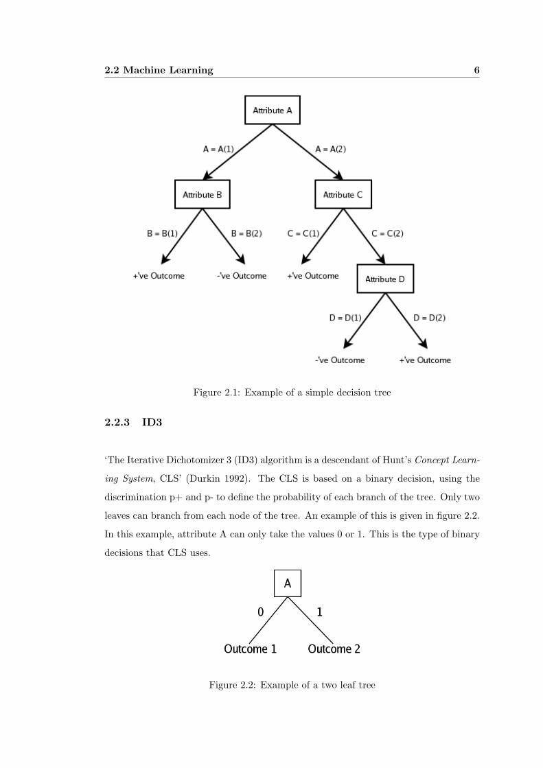
the top-down form given in figure 2.1, at the top is the first attribute and its values,

from this the next branch leads to either an attribute or an outcome. Every possible

leaf of the tree eventually leads to an outcome.

Figure 2.1 shows a simple decision tree, however in complex decision trees, the number

of attributes and their values can be very large. A decision tree can be generated quite

easily, but if the wrong attribute is used at the root, then the length of the tree can

become quite large. This property can be overcome by using entropy to determine

the information gain of each attribute. In order to minimise the size of the tree, and

minimise the number of attributes required, the attribute with the highest information

gain is used as the root of the tree.


Figure 2.1: Example of a simple decision tree

2.2.3 ID3

‘The Iterative Dichotomizer 3 (ID3) algorithm is a descendant of Hunt’s Concept Learn-

ing System, CLS’ (Durkin 1992). The CLS is based on a binary decision, using the

discrimination p+ and p- to define the probability of each branch of the tree. Only two

leaves can branch from each node of the tree. An example of this is given in figure 2.2.

In this example, attribute A can only take the values 0 or 1. This is the type of binary

decisions that CLS uses.

Figure 2.2: Example of a two leaf tree


The CLS algorithm according to (Durkin 1992):

Starting with an empty decision tree.

1. If all examples within the training set are positive,

then create a YES node and then stop.

If all examples within the training set are negative,

then create a NO node and then stop.

Else select an attribute A with values V1, V2, ..., Vnand create the desision node.

2. Arrange the training examples in to subsets C1, C2, ..., Cn of the training set C,

according to the values of V .

3. Apply Recursively to each of the training subsets Ci.

(Quinlan 1985) introduces the ID3 algorithm and presents the dilemma for decision

trees with large data sets. The feasibilty of such an approach to create a full set

of decision trees is unviable, therefore Quinlan presents the solution of entropy and

information gain.

ID3 was designed with these methods in mind to create a ‘desirable’ decision tree,

however it may not create the ‘best’ decision tree. That is the tree which comes to a

conclusion quickly and contains all of the desired rules. Quinlan introduces the training

set, which if carefully selected will then pass all of the desired rules to the algorithm. It

follows that a training set should be critically chosen. He also states that two different

sets of attributes and attribute values that lead to the same outcome are inadequate

for the training process.

According to (Quinlan 1985), in ID3, the training set is divided into subsets known as

windows. During the training process a window is chosen at random and this forms the

root of the decision tree. The window is formed into a tree and this tree is then tested

on the remaining objects within the training set. If this testing procedure succeeds then

the tree is satisfactory, if not, then the process iterates. This method is considered to

be much faster than creating a tree based on the entire training set.


2.2.4 Entropy

Quinlan (Quinlan 1985) introduces the process of information gain for the determina-

tion of the root of a tree. This method is used for arbitrary data sets. Given a set C

containing p objects of class P and n objects of class N.

The expected information is:

E(A) =∑V

i=1pi+nip+n I(pi, ni)

where I(p, n) = − pp+n log2

pp+n −

np+n log2

np+n

and the information gain:

gain(A) = I(p, n)− E(A)

2.2.5 Noise

Noise within the data set has to be dealt with, under most circumstances. This noise

includes misclassified information as well as missing information. Misclassification can

include incorrect nomeclature for attribute values, this arises when multiple people or

systems are used to collect data. Simple human error can add to misclassification. Two

modifiactions to the decision tree induction methods have been described by Quinlan,

(Quinlan 1985). These include:

1. The ability to decide whether certain attributes will present a true gain of accu-

racy to the tree, and

2. Inadequate attributes need to be dealt with, as noise can corrupt any data set.

(Quinlan 1985) presents an adaption of the information gain algorithm using the chi-

square test, to overcome the first situation. This method is favoured over the simple

addition of a percentage threshold for the information gain as this method can also

limit legitimate patterns. These methods help assure that ‘outliers’ are not included

within the data. The chi-square method determines the confidence that the attribute

can be rejected. This test gives the algorithm the power to determine whether further

developing of the decision tree will result in a more accurate tree. This eliminates


the risk of developing trees which encompass all possible situations including those

generated by noise.

The second situation can be corrected by assigning each leaf containing the attribute

with the noise to a class using the following tests: if p>n then assign to class P or

if p<n then assign to class N. This solution has been found to minimise the expected

error.

The ID3 algorithm as shown by (Durkin 1992) is:

1. Select a random subset of size W from the entire set of training examples. (select

a window)

2. Apply the CLS algorithm to form the decision tree or rule for the window.

3. Scan the entire set to find contradictions to the present rule.

4. If contraditions exist, incorporate these into the window and repeat from the rule

generation step.

2.2.6 C4.5

The C4.5 algorithm was also written by Ross Quinlan and finds its origin in ID3 and

CLS, according to (Quinlan 1993). It is also based on the binary descision basis seen

in CLS. The CLS algorithm is once again used to generate the initial decision tree

from the training set. C4.5 sees the introduction of the gain ratio criterion alongside

the information gain criterion for the selection of the most ‘useful’ attribute. The gain

criterion was found to be biased towards tests with several outcomes, (Quinlan 1993).

The information gain ratio criterion is given below:

gainratio(X) = gain(X)splitinfo(X)

where splitinfo(X) =∑n

i=1|Ti||T | × log2(

|Ti||T | )


2.2.7 Missing Values

Missing values within training sets can be managed by assigning values that are seen

in similar cases (Mitchell 1997). For example the value found that is most common

when another attribute matches that of a full record. This method requires some

inference into which attribute is most relevant to the missing attribute. According to

(Mitchell 1997), another method is to assign the average of the missing attributes that

correspond with another relevant attribute as above.

(Mitchell 1997) presents a third method, which is the method used within C4.5. The

attributes which contain missing values are given probabilities for each possible value.

When the missing value is being considered, the probabilities are assigned as values

of a new fractional attribute weighted by considering the aforementioned probabilities,

and the decision tree is created as normal (Quinlan 1985).

2.2.8 Continuous Data

Continuous data must be dealt with in decision tree induction in order to broaden the

potential of the method. Continuous data may be used easily after being discretised.

That is the data must be cut up into portions, depending on the immediate use of

the data. (Mitchell 1997) presents the method which dynamically defines new discrete

valued attributes that partition the continuous attribute value into a set of discrete

values. Consider a continuous valued attribute A and its set of two possible discrete

values where Ac is the threshold. That is A < c or the boolean opposite.

2.2.9 Discretization techniques

Several discretization techniques have been used within data mining. In order to pro-

vide categorical data sufficient for data mining, these techniques must be utilized on

continuous data. The methods being examined are relative to decision tree induction.

Partitioning of a continuous data set involves splitting the attribute on some random

threshold, finding the number of missclassified records and comparing this with another

split in order to find an acceptable threshold. Another method involves calculating the


mean of the data in question and choosing some distance relative to the mean as the

threshold. For example, all of the values that are greater or less than 12 a standard

deviation from the mean are considered one category and the remaining data would

be considered a different category. This method is described in figure 2.3. Take the

example of a range of temperatures, if the thresholds are set at, for example, 22o and

32o (the mean is 27o and one standard deviation is 10o), then the data can be split

into three categories, hot, mild and cool. The left hand shaded area would correspond

to the cool data, the unshaded to mild and the right hand shaded section is the hot

area. In a binomial distribution as presented in figure 2.3, the mean, x of the data is

found in the center of the distribution. The upper and lower thresholds are found by

taking the standard deviation of the distribution and adding or subtracting this from

the mean respectively. These calculations are presented below.

mean x =∑

x

N

where

• x is the value of each record and,

• N is the total number of records

standard deviation σ2 =∑

(xi−x)2

N

where

• σ2 is the square of the standard deviation

• x is the mean

• xi are the record values

• N is the number of records

Other methods of splitting continuous data include using the variance or the gini index

to determine the best split. However these methods provide no way to compare the

splits on discrete data.

2.3 Artificial Neural Networks 12

Figure 2.3: Standard deviation descretization method

2.3 Artificial Neural Networks

Neural networks are designed to mimic the neurons within the human nervous sytem,

according to (Rojas 1996). One must understand how these systems work to fully

understand the workings of artificial neural networks. Biological neural networks are

systems of signals which are forwarded from neuron to neuron. ‘Neurons receive signals

and produce a response’ (Rojas 1996). In general, information comes into the motor

neuron via dendrites. These dendrites receive the information via the synapses, which

can be considered as storage mechanisms. The synapses distribute the information

between independent neurons. At the center of the neuron are the organelles, which

provide the neurons with all of the requirements for survival. Also the mitochondria

supply the energy to keep the cell working. Axon’s transmit the output signals made

by the neurons. Each cell may only have one axon, according to (Rojas 1996). Some

cells however do not have an axon as they are only required to link two sets of cells.

(Rojas 1996) states that artificial neural networks are similar to biological neural net-

works in that they have inputs, an output and a working body. The synapses are

simulated via weightings on the external and internal input and output channels. Fig-

ure 2.4 is an adaption of an abstract neuron as described in (Rojas 1996). It describes

a simple model of a neuron, having xi as the inputs, wi as the weighting and f is the

output of the neuron.(Where f =∑i

0 xiwi)

According to (Rojas 1996), a neural network can be thought of as containing many of


Figure 2.4: Example of a back propagation neural network

these nodes which are interconnected.

(Rojas 1996) introduces several types of neural networks, and there are many in ex-

istance. However, only the Back Propagation neural network will be examined here.

A typical back propagation network will be similar to figure 2.5. Figure 2.5 has been

adapted from (Widrow & Lehr 1990).

Figure 2.5: Example of a back propagation neural network

Neural networks consist of neurons, that have a number of weighted inputs and only

a single output. The typical network is a grouping of interconnected neurons with the

input layer of neurons outputs connected via a weighting term, to the inputs of the next


layer. The final layer is the output layer and the layers between input and output are

known as hidden layers. The layout of a network ensures difficulty in understanding

the method of which artificial neural networks use. This creates the notion that neural

networks are an abstract method of learning.

Training a neural network entails determining the most effective values for the weights

of each input. A neuron must also contain a single unit input as well as all variable

inputs. The training method being analysed here is backpropagation.

2.3.1 Backpropagation

(Werbos 1990) states that backpropagation is a method that finds just one of its uses

within neural networks. Backpropagation or feed forward, is a method of determining

the parameters required for an efficient neural network. (Werbos 1990) states, ‘back-

propagation is simply an efficient and exact method for calculating all the derivatives of

a single target quantity with respect to a large set of input quantities’.(Rojas 1996) in-

troduces feed-forward networks as a form of ‘threshold logic’. Backpropagation is a form

of supervised learning, with the goal of modifying the neural network so that its actual

outputs approach a desired set of outputs (Werbos 1990). According to (Rojas 1996)

threshold logic is based on computer logic decisions with the added threshold used to

compare continuous inputs. According to (Rojas 1996) neural networks can be thought

of as a black box approach to learning. (Werbos 1990) introduces the sigmoidal func-

tion as the most common transfer function used in backpropagation.

The Sigmoid function: f = 11+e−Z , where z =

∑i0 xiwi. The sigmoid function outputs

values between 0 and 1 (Mitchell 1997).


Figure 2.6: The Sigmoid function

2.3.2 Multilayer Networks

Single layer networks are only capable of expressing linear decisions (Mitchell 1997).

Multilayer networks provide nonlinear decisions.

2.3.3 Training Neural Networks

Neural networks must be set up such that a set of inputs will produce a desired set of

outputs (Krose & van der Smagt 1996) . In order for neural networks to become efficient

in their decision making, they must be trained correctly and efficiently. The amount

of training time required varies greatly from seconds to hours. However the method

reduces the effect of overfitting and the training time required is overcome by the fast

evaluation made by the properly trained network. (Mitchell 1997) presents gradient

descent as the training method used within backpropagation. The gradient descent

method converges on local minima (Mitchell 1997). This property can be overcome in

most situations by adding a momentum term. This term tends to cause the iterations to

converge on global solutions rather than local solutions. The backpropagation function

(Mitchell 1997) using a momentum term is given below.

The backpropagation rules for updating weights can be described by:

∆wji(n) = ηδjxji + α∆wji(n− 1)

Where:


• ∆wji(n) are the updated weights

• α is the momentum constant, ranging between 0 and 1

• η being the learning rate

• δj is the error term

• xji is the input from node i to unit j

ηδjxji updates the weights, while α∆wji(n− 1) provides the momentum to ensure a

global solution. (Mitchell 1997)

The backpropagation method consists of updating the weights in order to change the

output of the network. The weights are updated until convergence of the weights has

been made. If convergence is not made, then training should be stopped after some

number of iterations. Convergence can be seen either locally or globally, therefore the

momentum term is added in order to prevent local convergence. Firstly the weights are

set at some arbitrarily chosen values, and the output of the network is examined. The

weights are then adjusted in order to bring the outputs closer to their desired values.

The weights are adjusted in this manner until an acceptable group of outputs are found

or the number of iterations reaches some pre set limit.

2.3.4 Applications of Neural Netwoks

Neural networks in particular have extensive applications within the engineering indus-

try. These include the unsupervised learning of physical limits for industrial robots.

(Mitchell 1997) gives an example of the automatic steering of an automobile using

neural networks. The ALVINN system, which used the feed forward type of neural

network, taking in images from a front mounted camera could steer the automobile

effectively at speeds of up to 110 km/h.

Other examples provided by (Mitchell 1997), that carry some success, include hand

writing recognition, face and speech recognition.

Chapter 3

Methodology

3.1 Program Methodology

3.2 Decision Tree Induction

Implementation of the ID3 algorithm to build a decision tree for given categorical data

is the initial aim of this project. The ID3 algorithm was considered to be an appropriate

algorithm for implementation due to its simplicity. The C4.5 algorithm contains the

ID3 algorithm and some efficiency improvements, as well as adaptions for handling

missing data, noise and other expected problems.

The algorithm used to provide the base for this project is given below:

1. Input the attributes, target attribute and examples

2. Create a node

3. Test if all the attributes have the same outcome, if yes return the outcome and

exit

4. Test if attributes array is empty, if yes return the most common value of the

target attribute and exit

5. Find the attribute with smallest entropy

3.3 Program Modules 18

6. Create a group of subsets for each value of the best attribute

7. For each non-empty subset send the subset as examples to step 1

This can be represented visually in the flow chart provided in figure 3.1.

3.3 Program Modules

3.3.1 Data Input Methods/Data Structure

In order to manipulate any data, it must be imported into the working environment.

For ease of use and simple pre-processing on the data, the input files are in the Microsoft

Excel format. Matlab uses the xlsread function to read the data into its workspace.

The data is split into two separate Excel files. One file contains the data to be anal-

ysed, with the attributes in the columns, records in the rows and the final column being

the outcomes. The second file is similar to the C4.5 names file, in the manner that it

contains the attributes and attribute values that correspond to the data.

The files have the respective filenames of:

• filename.xls

• filename.types.xls

The term types was used as to highlight the differences between the names and types

files.

Table 3.1 shows an example of the layout of a typical data file and table 3.2 shows the

types file for this data set.

Table 3.1 is the simple data set used for verification of the algorithm. The data consists

of four attributes, outlook, temperature, humidity and wind, in the first four columns


Figure 3.1: Flow chart representing the ID3 algorithm


Sunny Hot High Weak Don’t Play

Sunny Hot High Strong Don’t Play

Overcast Hot High Weak Play

Rain Mild High Weak Play

Rain Cool Normal Weak Play

Rain Cool Normal Strong Don’t Play

Overcast Cool Normal Strong Play

Sunny Mild High Weak Don’t Play

Sunny Cool Normal Weak Play

Rain Mild Normal Weak Play

Sunny Mild Normal Strong Play

Overcast Mild High Strong Play

Overcast Hot Normal Weak Play

Rain Mild High Strong Don’t Play

Table 3.1: A typical input data set

and the final column contains the outcome, which can be to play golf or don’t play golf.

The next data set is the description of the possible attribute values for each attribute.

Sample data is provided in table 3.2. The first column consists of the name of each

attribute and each consecutive column contains a possible value for each attribute. As

can be seen in table 3.2 the number of values for each attribute can vary, therefore the

data set is not necessarily square. Therefore looking at row three and the attribute

humidity, the values that are possible are high and normal.

Outlook Sunny Overcast Rain

Temperature Hot Mild Cool

Humidity High Normal

Wind Weak Strong

Table 3.2: The types file for the data in table 3.1


These files are imported into the matlab workspace by the functions getdata(filename),

getvalues(filename) and gettypes(filename). The getdata function imports the examples

and stores these in an array. gettypes retrieves the attributes and getvalues retrieves

the attribute values.

Unknown data is handled by the function replace missing data(). Any missing values

found within the examples data set are replaced with the most common value for that

particular attribute. This is a crude method of dealing with missing data, however it

is sufficient for an initial version of the algorithm. The training and testing data shall

be carefully chosen in order to eliminate the possibility of operating on missing data.

A variable named data type was created in order to handle both numerical and string

categorical data. For example, an attribute can have the values of sunny, overcast and

rain or 1, 2, and 3. Continuous data is to be handled separately. In order to make

a decision based on continuous data one or more best split thresholds must be found.

Once these thresholds are determined, the data can be split into discrete attribute

values, for example if humidity ≥ 75% then humidty is high otherwise humidity is

normal. These values then can be parsed to the decision tree algorithm.

The main algorithm is located in id3(). This algorithm follows the steps outlined below.

1. If there are no examples present then break

2. Remove the subset that was previously examined (if applicable)

3. Let examples equal the first set contained in examples now via choose set()

4. Save this set to file filename.set via write set()

5. Determine the entropy for each value and find the attribute with the smallest

entropy using find entropy

6. Write the leaf information to the tree and add the best attribute

7. Create a reference row to be used in finding each subset in examples now using

create ref point

8. Add subsets to examples now for each value of the best attribute that does not

have an outcome. If an outcome is present then this is reported in the tree


otherwise an identifier (discussed later) is placed in the tree for this attribute

value.

9. Remove the attributes that have been used in this branch via remove attributes

10. Return to step 1 using the examples now as the current example set

The function choose set takes the examples, attributes and outcome arrays as inputs.

From the example array the function finds the first ‘eor’ (end of records or 12345 if

numerical data) index in the data set, it then saves the rows of data from the first row

up to the first index as the example set to be examined. This acts as a shift register

in order to keep all examples in one array but only operate on the subset that is in

question. Similarily the outcome array is divided up in the same manner. The column

corresponding to the previous attribute in the tree is also removed so that it cannot

occur more than once in the same branch. These arrays are then returned back to the

id3() algorithm.

write set is used to save each subset being examined, to file. The file can be used for

backtracing and verification purposes. The output of this function is provided in table

3.3.

3.3.2 Data Output Method/Structure

The output method employed by the matlab algorithm is the use of the fprintf function

to write the results to file. This allows for simple extraction of the data and allows the

data to be examined outside of the matlab program.

The output files include:

• filename.set

• filename.tree

• filename test.dat

• filename train.dat


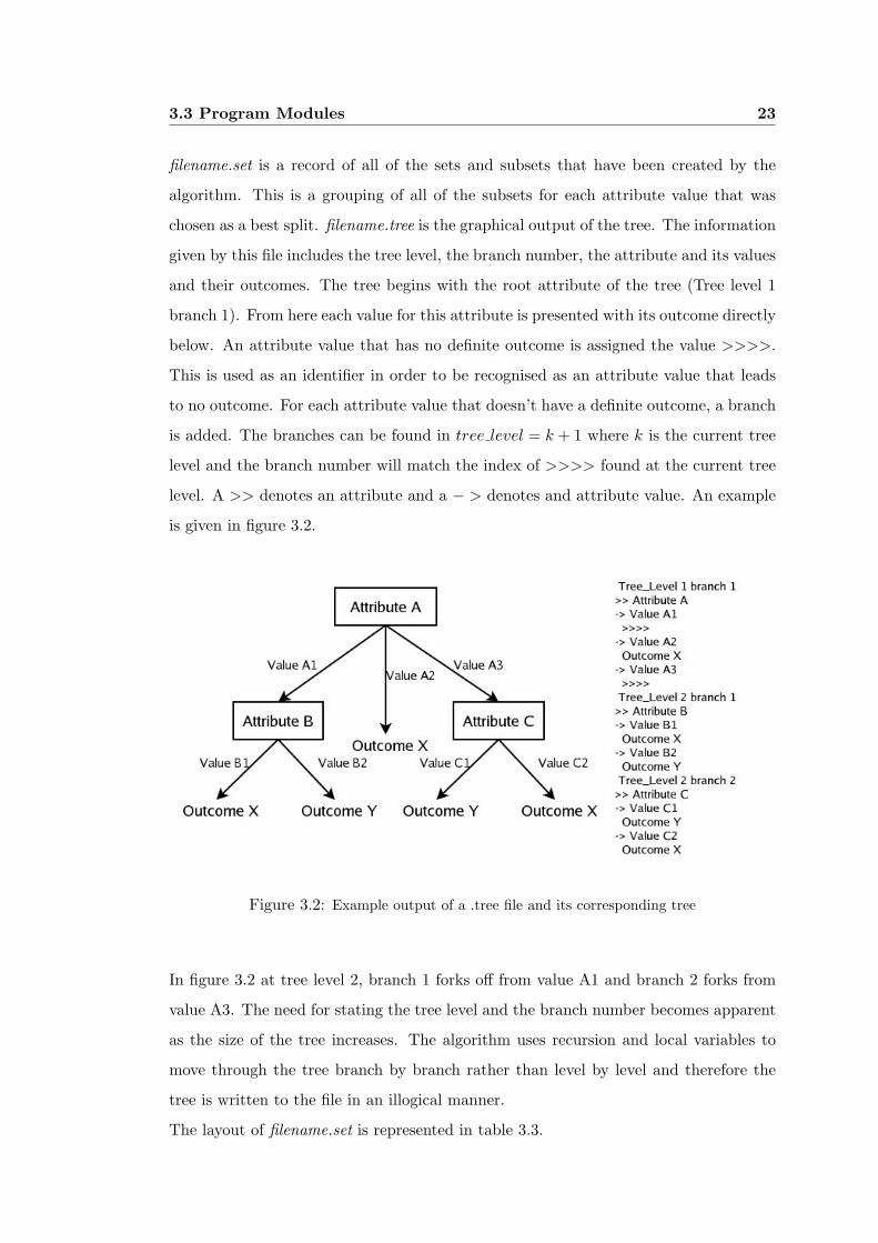
filename.set is a record of all of the sets and subsets that have been created by the

algorithm. This is a grouping of all of the subsets for each attribute value that was

chosen as a best split. filename.tree is the graphical output of the tree. The information

given by this file includes the tree level, the branch number, the attribute and its values

and their outcomes. The tree begins with the root attribute of the tree (Tree level 1

branch 1). From here each value for this attribute is presented with its outcome directly

below. An attribute value that has no definite outcome is assigned the value >>>>.

This is used as an identifier in order to be recognised as an attribute value that leads

to no outcome. For each attribute value that doesn’t have a definite outcome, a branch

is added. The branches can be found in tree level = k + 1 where k is the current tree

level and the branch number will match the index of >>>> found at the current tree

level. A >> denotes an attribute and a − > denotes and attribute value. An example

is given in figure 3.2.

Figure 3.2: Example output of a .tree file and its corresponding tree

In figure 3.2 at tree level 2, branch 1 forks off from value A1 and branch 2 forks from

value A3. The need for stating the tree level and the branch number becomes apparent

as the size of the tree increases. The algorithm uses recursion and local variables to

move through the tree branch by branch rather than level by level and therefore the

tree is written to the file in an illogical manner.

The layout of filename.set is represented in table 3.3.


Outlook Temperature Humidity Wind Outcome

Training Set sunny mild high weak 0

sunny hot high strong 0

rain mild high strong 0

rain cool normal strong 0

rain mild normal weak 1

overcast cool normal strong 1

rain mild high weak 1

overcast hot high weak 1

sunny mild normal strong 1

overcast mild high strong 1

sunny cool normal weak 1

Temperature Humidity Wind Outcome

Sunny Subset mild high weak 0

hot high strong 0

mild normal strong 1

cool normal weak 1

Temperature Wind Outcome

Rain Subset mild strong 0

cool strong 0

mild weak 1

mild weak 1

Table 3.3: Listing of the file golf.set

The file filename.set consists of three space delimited tables that represent the subsets

that the ID3 algoritm has operated on. This includes the original full set of data and a

subset of the data that contains the sunny attribute value and one that contains the rain

value. From these subsets, it is easy to see how a decision is made on which attribute

is best. In the sunny subset, when the humidity is high an outcome of 0 or don’t play

is reached while the humidity is normal an outcome of play is reached. Therefore the

attribute humidity contains enough data to make a decision depending on the state of

the humidity. The same process can be applied to the wind attribute in the rain subset.


The files filename test.dat and filename train.dat contain a listing of the data used to

test and train the decision tree respectively. The data is in a space delimited format

for ease of import into the MS excel format. The order of the data is the same as that

of the input data mentioned previously.

3.3.3 Continuous Data

In order to represent continous data in a form which can be compared with the cat-

egorical data, the standard deviation technique of discretization will be implemented.

This is considered a preprocessing technique, and therefore will be only an appendage

to the ID3 algorithm. The algorithm takes in the column of discrete data and returns

the data in three categories, high, moderate and low. The function has the following

inputs and outputs:

[categories] = discretize{thiscolumn, percentdeviation} Where:

• categories is the array of discrete data to be parsed into the ID3 algorithm

• thiscolumn is the column of continuous data that is to be discretized

• percentdeviation is the percentage of the standard deviation that will be used to

create the upper and lower decision thresholds (suggested value = 50%)

In order to use the discretized data in the ID3 algorithm, the types file must be edited

manually to contain the values high, moderate and low.

The discretization module uses two thresholds to partition the data in to three parti-

tions. The mean of the data is found and thresholds are made at a percentage of the

standard deviation on either side of the mean. The mean and standard deviation are

included in the matlab language and therefore do not need to be implemented. Some

control over the size of the partitions is gained by using an index which is relative to

the size of the standard deviation. Thereby creating a partition that can be resized

to better describe the data. The need for this control arises when the data contains

outlying values and therefore is not described well by the normal binomial distribution.

3.4 Data mining utilities within Matlab 26

Improvements could be made on this method, however the data being examined at this

stage is categorical and therefore more complex methods have not been examined.

The discretisation method has been tested using the data in table 3.4 and the outputs

of the function are also provided here. The thresholds found for this set of data were

high = 0.6690 and low = 0.0324. The data is simply a group of twenty-five randomly

generated numbers that lie between zero and one. MATLAB’s rand() function was used

to generate the numbers. The mean has then been taken and the standard deviation

found. A percentage of the standard deviation is used to place the thresholds thereby

resizing the moderate field. In this case a half of a standard deviation was taken (50%).

The thresholds are found in this manner and any records that have values larger than

the upper threshold, are replaced with ’high’, any values lower than the lower threshold

are replaced with ’low’. The values in between the two thresholds are replaced with

’moderate’.

From the data given in table 3.4 the most common values are moderate values. In

order to even out the distribution, the percentage of the standard deviation should be

lowered in order to shorten the ’spread’ of the moderate threshold.

3.3.4 Rule Contradictions

Contradictions to some rules exist in real life data. However at this initial stage of the

algorithm, contradictions have not been dealt with fully.

3.4 Data mining utilities within Matlab

3.4.1 Neural Network Toolbox

The Neural net toolbox incorporated within matlab, consists of implementations of

various architectures. In this study, the most commonly used backpropagation network

is being examined. The neural network toolbox consists of functions as well as a gui

implementation. The first step in building a network is defining the network. This is

done via the newff function.


Input data Output data

0.8529 ‘high’

0.1803 ‘moderate’

0.0324 ‘low’

0.7339 ‘high’




0.0129 ‘low’

0.8892 ‘high’

0.866 ‘high’







0.8636 ‘high’


0.9805 ‘high’

0.7918 ‘high’


0.833 ‘high’



0.669 ‘high’

Table 3.4: Discretisation module output


A description of the arguments parsed to this function follows:

net = newff(data limits,[neurons in first layer,neurons in second layer]{transfer func-

tion for hidden layer,transfer fuction for output layer}, training method)

1. Data limits: the minimum and maximum value for each attribute value

2. Neurons in each layer defines the architecture of the network

3. Transfer functions: the transfer functions used to train the network

4. Training method: defines which training algorithm will be used

The possible values for these arguments are:

1. Continuous values or 0 and 1 for categorical data

2. Typical networks should only have one hidden layer and the output layer. The

number of neurons required varies with the size of the data.

3. The transfer functions provided within matlab are: tan-sigmoid, log-sigmoid and

pure linear.

4. The methods for training are either the gradient descent method or the gradient

descent method with a momentum term

The network once defined can be modified to define a customised network that is

suitable for the data being used. The parameters that will be of interest for this

project are:

1. net.trainParam.lr, the learning rate which determines the step size for adjusting

the weights

2. net.trainParam.mc, the momentum constant which modifies the learning rate

depending on the gradient of changes in the weights

The next step in building a network within matlab is to train the new network using

the function train.


[net,tr] = train(net,p,t)

Where:

• net is the network created with the newff

• tr is the training record (performace feedback)

• p is the training data

• t is the training outcome data

The data that is input into the neural network via the variables p and t can be of two

forms, either continuous data within a range or binary data for categorical variables.

The comparison between the decision tree output and the neural network outputs

concerns categorical data. In order to describe a catergorical set of attribute values in

binary form, they must first be split up into an array the size of the total number of

values for the concerned attribute. For example, examining the outlook attribute from

the golf set, there are three possible values that the outlook can take. These values are

sunny, overcast or rain. Table 3.5 describes how each of these values would be input to

the network.

Value Sunny Overcast Rain

Sunny 1 0 0

Overcast 0 1 0

Rain 0 0 1

Table 3.5: Binary input into the neural network

The rows contain the inputs given to the network. If the outlook is sunny then the

sunny column must have a value of 1 and the rest must be 0. In this way it is not

possible to be sunny and overcast. This method does ensure the integrity of each value

is sustained however the number of inputs to the network can become extremely large.

Consider the temperature attribute. This may be described by a single continuous

variable or this variable could be divided into categories such as hot, mild and cool. In

this simple example the number of variables input to the network is increased three-

fold.


The outputs of the network can be described in a similar manner. Because the output

of the network should be play or don’t play, a variable for each outcome is created.

Therefore a play outcome is made from an output of the network given as [1 0] and

don’t play would be [0 1]. This is a novel method, however the output of the network is

very rarely as neat as [0 1]. More likely values may be [0.12 0.94], this property may be

overcome by rounding these values to the nearest whole number. However this does not

describe the actual output of then network when a value of say [0.58 0.47] is produced.

This value would most likely mean that the data is inconclusive, but the chances are

an outcome of play will be reached. In order to monitor this property, we introduce a

‘confidence’ value. The confidence is simply the absolute value of the difference between

the two values. in this case the confidence would be 0.58− 0.47 = 0.11 whereas the

earlier values would give confidence = 0.94− 0.12 = 0.82. From the two values it can

be seen that there is more confidence in the outcome being don’t play for the first

example than there is for the play outcome of the second example.

In order to test the network, the sim function needs to be called. This function simulates

the network with regards to the single input record that is given to it. The testing

data should contain several records while each of these should be presented to the sim

function seperately. The inputs and outputs to the sim function are given below.

outcome = sim(net, test)

Where:

• outcome is the outcome presented by the network

• net is the network created with newff

• test is the data that is being examined

In order to produce a binary outcome, the outcome variable is subjected to the round

function, however firstly the confidence must be found. These outcome values can

then be replaced with their respective values, for example ‘play’. If the outcome does

not correspond to one of the outcome values, then the value should be presented as

‘inconclusive’.

The structure of the network that was used for comparison was found by trial and


error. This structure consists of six hidden neurons and two output neurons. It can be

best described by figure 3.3.

Figure 3.3: Neural network used for comparison

Chapter 4

Results

4.1 Decision Tree Induction Implementation

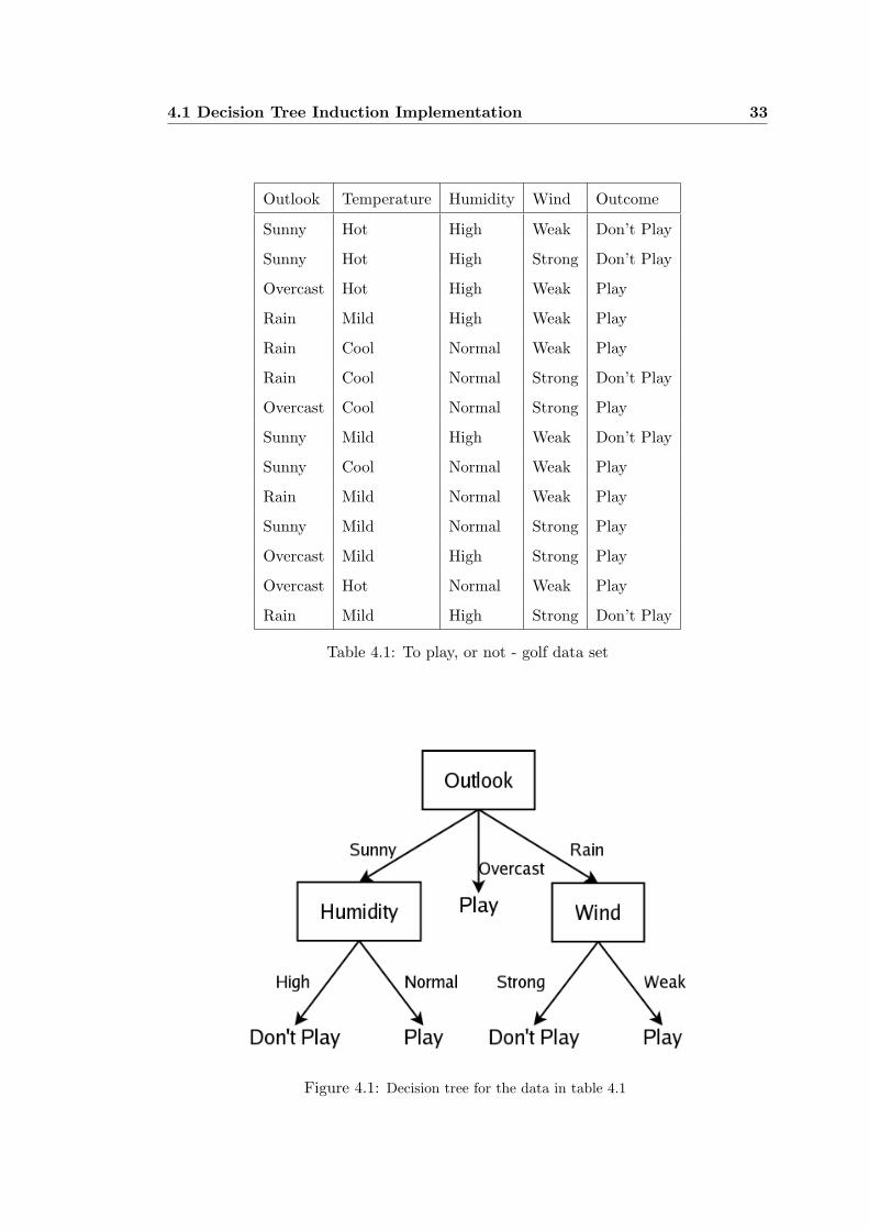
4.1.1 Example Data

The training data being used to initially verify the decision tree algorithm and the

neural network method is given in table 4.1. This trivial data set has four attributes

and two possible outcomes. The outcome will either be to play golf (Play) or not to

play golf (Don’t Play). The attributes and their corresponding values follow, Outlook -

{sunny}, {overcast}, {rain}, Temperature - {hot}, {mild}, {cool}, Humidity - {high},

{normal} and Wind - {strong}, {weak}.

The C4.5 decision tree given for this data set is shown in figure 4.1.

Another data set that will be examined is the vote data set. The vote set is included

with the C4.5 distribution. It originates from voting records taken from the congres-

sional quarterly almanac in the 98th congress (2nd session 1984, volume XL). The data

describes the votes by each U.S. house of representatives congressmen on sixteen issues.

Each vote has a value of yes, no or undecided. The possible outcomes for each voter is

either a democrat or a republican congressman. The data consists of sixteen attributes

(issues) each with three values. There are 300 records in the set. The set is known

4.1 Decision Tree Induction Implementation 33

Outlook Temperature Humidity Wind Outcome

Sunny Hot High Weak Don’t Play

Sunny Hot High Strong Don’t Play

Overcast Hot High Weak Play

Rain Mild High Weak Play

Rain Cool Normal Weak Play

Rain Cool Normal Strong Don’t Play

Overcast Cool Normal Strong Play

Sunny Mild High Weak Don’t Play

Sunny Cool Normal Weak Play

Rain Mild Normal Weak Play

Sunny Mild Normal Strong Play

Overcast Mild High Strong Play

Overcast Hot Normal Weak Play

Rain Mild High Strong Don’t Play

Table 4.1: To play, or not - golf data set

Figure 4.1: Decision tree for the data in table 4.1


to contain some contradictory records, however there are no missing records or values.

The voting data can be used to determine which party a congressman may originate

from by examining their voting trends over the sixteen issues. From these trends it may

be inferred that the voting trends followed may be simillar for each particular member

of a party. Some noise exists in the data in the form of conflicts of interest that may

be realised by some congressmen. The issues were deemed key votes for this session by

the congressional quarterly almanac. Clarification of the voting data may be found in

appendix B.1.

4.1.2 Verification

The verification using the simple golf data set is also backed up by comparisons of the

C4.5 output for each data set being examined.

The actual C4.5 output follows. From this the tree was interpreted and compared with

the output found in golf.tree, created by matlab.

Decision Tree:

outlook = overcast: yes (3.0)

outlook = sunny:

| humidity = high: no (3.0)

| humidity = normal: yes (2.0)

outlook = rain:

| windy = strong: no (2.0)

| windy = weak: yes (2.0)

The rules for this data set can then be interpreted as:

1. If Outlook is Sunny and Humidity is High then Don’t play

2. If Outlook is Sunny and Humidity is Low then Play

3. If Outlook is Overcast then Play

4. If Outlook is Rainy and Wind is Strong then Don’t play


5. If Outlook is Rainy and Wind is Weak then Play

From these rules, verification of the neural network can be made. This will follow in

the next section.

Listing 4.1.2 is the decision tree created by the matlab algorithm.

Tree_Level 1 branch 1

>> outlook

-> sunny

>>>>

-> overcast

yes

-> rain

>>>>


>> humidity

-> high

no

-> normal

yes


>> wind

-> weak

yes

-> strong

no

The parameters used to generate this tree were, precisionthreshold = 0 and percenttotrain = 100.


As there were no contradictions within the data the whole data was used as the training

window. The verification for this example may therefore be considered trivial as the

test data was used to train the algorithm, however the aim of this experiment is to

identify the correctness of the tree versus the known correctness of the C4.5 generated

tree.

The decision tree generated by the matlab algorithm is the same as the C4.5 tree and

therefore the rules must be the same.

The voting data set was analysed, two subsets of the data set were created for training,

and the remaining records in each case were saved for testing purposes. In both cases

40% of the full data set was chosen as a window. 75% of this data was used for building

the decision tree and 25% kept for verification. Such a small percentage of the data

was used for training because of the existance of contraditions in the data. A smaller

training portion realises less contradictions. The subsets were also written to files in

order to use the same training set for building the C4.5 tree as well as for use with

the neural network method. The tree obtained in matlab for the first case study is

provided in appendix C. The graphical representation is shown in figure 4.2

Figure 4.2: Decision tree for a subset of the voting data created in matlab


The data does contain some contradictory data as can be seen from the C4.5 output

given in appendix C. The graphical representation is provided in figure 4.3. The

superfund right to sue yes and undecided branches both have one record that doesn’t

support the outcome. C4.5 uses pruning techniques to reduce the size of the tree. This

leads to the tree being cut off at the third level, rather than progressing into the fourth.

The pruning confidence level can be set for C4.5 to reduce this effect, however this is

not recommended for larger trees. The yes vote in question has one record out of eight

that does not support the outcome of republican, conversely the undecided vote has

one contradiction out of two.

Figure 4.3: Decision tree for a subset of the voting data created using C4.5

It can be noticed from the two trees that the same rules can be generated although the

matlab tree has more attributes to be examined. One way to simplify the tree would

be to remove the fourth level and replace this with the most common outcome for the

attribute. This leads to the trees being matched exactly.

C4.5 implements further pruning of the trees, however in this example the difference

between the two trees is trivial as a tree with ten branches is sufficiently small for quick

analysis. The options that were parsed to the C4.5 program use the information gain

method rather than the information gain ratio method. The matlab algorithm uses

information gain. The C4.5 program also created ten trees, in order to create at least


one tree that was similar to the matlab generated tree. C4.5 generates different trees

depending on the window it chooses to begin with. From the matlab voting tree, the

following rules can be manually extracted.

1. If Physician fee freeze is No then congressman is Democrat

2. If Physician fee freeze is Yes and immigration is No and Superfund right to sue

is No then outcome is Democrat


is Yes and Mx missile is No then outcome is Republican


is Yes and Mx missile is Yes then outcome is Democrat


is Yes and Mx missile is Undecided then outcome is Republican

6. If Physician fee freeze is Yes and immigration is No and Superfund right to sue is

Undecided and Adoption of the budget resolution is No then outcome is Democrat


is Undecided and Adoption of the budget resolution is Yes then outcome is Re-

publican


is Undecided and Adoption of the budget resolution is Undecided then outcome

is Democrat

9. If Physician fee freeze is Yes and immigration is Yes then outcome is Republican

10. If Physician fee freeze is Yes and immigration is Undecided then outcome is

Republican

11. If Physician fee freeze is Undecided and Handicapped infants is No then outcome

is Democrat

12. If Physician fee freeze is Undecided and Handicapped infants is Yes then outcome

is Democrat

13. If Physician fee freeze is Undecided and Handicapped infants is Undecided then

outcome is Republican

In order to verify the rules, the test data is compared against the rules that have been

generated. Thirty records will be examined as this equates to 25% of the subset chosen

to build the tree.

The records are given in appendix B.2. The records have been grouped into subsets in

order of the relevant attributes. These subsets are presented in table 4.2.

Attributes Values Outcome Actual Outcome Instances

Physician Fee Freeze Undecided

Handicapped Infants Undecided Republican Republican 1

Physician Fee Freeze No Democrat Democrat 21

Physician Fee Freeze Yes

Immigration Yes Republican Republican 6


Immigration No

Mx Missile No Republican Republican 2

Table 4.2: Test results using the matlab algorithm

Analysing the test data it was found that 100% of the records complied to the rules

that had been extracted. This is reinforced by the fact that the number of records in

the test data was relatively small.

The second case study produced the two decision trees found in figure 4.4 and figure

4.5.

From the trees it can be seen that the pruning and windowing methods create a smaller

tree although the rules will generally be the same. As before matlab creates a tree that

complies to all rules found in the training set whereas C4.5 generalises the rules that

are not commonly encountered.

The rules that can be interpreted from the second matlab tree are presented in table

4.3.


Figure 4.4: Decision tree for the second subset of the voting data created in matlab

Figure 4.5: Decision tree for the second subset of the voting data created using C4.5


Attributes Values Outcome Actual Outcome Instances

Physician Fee Freeze No Democrat Democrat 14

Physician Fee Freeze No Democrat Republican 1


Duty Free Exports No

Adoption of the Budget Resolution No Republican Republican 12



Adoption of the Budget Resolution Yes Republican Republican 1



Adoption of the Budget Resolution Undecided Democrat Na 0


Duty Free Exports Yes

Handicapped Infants No Democrat Democrat 1



Handicapped Infants Yes Republican Na 0



Handicapped Infants Undecided Democrat Na 0


Duty Free Exports Undecided Republican Na 0

Physician Fee Freeze Undecided Democrat Democrat 1

Table 4.3: Count of correct test records against the rules generated from the second

case study


Analysing the data presented in table 4.3 it can be seen that the tree gave one incorrect

prediction concerning the test data. This equates to 96.7% correct predictions. Taking

into account the first case study gave 100% correct and the second gave 96.7%, the

decision trees results are reliable on these moderate sized data sets. The data from

these case studies will now be evaluated using the neural network method.

4.1.3 Neural Network Method

The initial verification of the neural network method in matlab was done using the

golf data set presented in table 4.1. The network used was a backpropagation network

using the tan-sigmoid transfer function. The training method is gradient descent with

momentum. The network contains six neurouns in the hidden layer and two output

neurons. The data structure for the network is in the binary form where each categorical

value has its own bit. The bits are allocated as in the following set [sunny overcast rain

hot mild cool high normal weak strong]. For example, the set {sunny,hot,high,weak}

will be [1 0 0 1 0 0 1 0 1 0]. The outcome is in the same form with a neuron for each

possible outcome, [Play Don’t Play]. Therefore the example set given should result in

the output [0 1], that is don’t play.

Training a network correctly proves to be more effective using trial and error methods.

Analysing 75% of the golf data, a network was found that had 100% correct outcomes

for the training and test sets. However an incorrect outcome was given for one record

that was not part of the test or training data.

The record was:

Outlook: rain, Temperature: mild, Humidity: normal and Wind: strong

This record gave an outcome of play when the decision tree method gives an outcome of

don’t play. The incorrect outcome for this record gave a percentage of precision for the

neural network method of 87.5%. This is out of only eight records and therefore carries

little weight, however it is sufficient for verification of the method of data input. This

record may be trivial as there are no actual records which contain the data, however

using some intuition, any weather conditions that contain strong winds should lead to

4.2 Method Comparison 43

a no play outcome when considering the game of golf.

The output of the script used, netgolf.m is provided in appendix D.1.

4.2 Method Comparison

4.2.1 Comparision Data

The data being used for comparison of the two methods is the voting data mentioned

in section 4.1.1. The subset of the data being used has 120 records with 30 of these

reserved for testing.

4.2.2 Neural Network Outputs

The comparison technique consists of building a decision tree using the algorithm de-

veloped in matlab and comparing the rules found with the outputs given by using the

neural network toolbox. The two methods have been outlined in previous sections. A

percentage of difference between the outcomes of the two methods was found.

The data shown in table 4.4 represents the outcomes and expected outcomes for five

trained networks. The data consists of an outcome for each test record in each trial

and a confidence for each of these records. Each trial consists of the same network (de-

scribed later) with the only difference being the initial weights of the neurons. A value

of confidence was introduced in order to rank the accuracy of each outcome that was

found. The confidence is made up of the maximum outcome value minus the minimum

outcome value in the outputs of the network. For example if a record has an outcome

of [0.1 0.9] then a confidence of 0.9− 0.1 = 0.8. This value therefore represents the

accuracy of each outcome that has been predicted.

All of the example networks had incorrect predictions. Network four was the only

network that did not give an incorrect prediction for record 21. This suggests that

while the decision tree method only concentrates on consecutive best attributes, the

neural network method examines all of the data. There is most likely an attribute that


weighs more heavily on the outcome in the neural network that is not considered in the

decision tree method. Network one had incorrect predictions for the records number

six and twenty-one, while network three gave records thirty and twenty one incorrect

predictions. Network trials two, four and five had only one incorrect prediction, and

therefore are better trained networks. Of these networks, trial four presented the

incorrect prediction with the lowest confidence, this suggests that it is the most correct

network. The parameters used for training the networks were as below:

• Number of hidden neurons = 6

• Number of output neurons = 2

• net.trainParam.lr = 0.4

• net.trainParam.mc = 0.3

• net.trainParam.epochs = 500

The training script netvote is provided in appendix E.2.1.

These parameters were chosen by trial and error. The number of hidden neurons was

varied between three and twelve neurons, without much change being experienced.

The momentum constant was varied from 0.1 to 0.9 without much improvement in

any direction. The learning rate was also varied and it was found that the network

converges quickly and directly at a value of 0.4. The network seems to converge well

with these values and with the number of epochs (total number of iterations before

breaking) set at 500.

Tri

alO

neT

wo

Thr

eeFo

urFiv

eA

ctua

l

Rec

ord

Con

fiden

ceO

utco

me

Con

fiden

ceO

utco

me

Con

fiden

ceO

utco

me

Con

fiden

ceO

utco

me

Con

fiden

ceO

utco

me

Out

com

e

11.

11re

p1.

22re

p1.

04re

p1.

21re

p1.

20re

pre

p

21.

00de

m1.

05de

m1.

04de

m1.

03de

m0.

96de

mde

m

31.

13re

p1.

03re

p1.

13re

p1.

12re

p0.

85re

pre

p

41.

06re

p1.

21re

p1.

18re

p0.

93re

p0.

90re

pre

p

51.

02de

m1.

01de

m1.

04de

m1.

03de

m1.

01de

mde

m

60.

21re

p0.

87de

m0.

58de

m0.

56re

p0.

30de

mde

m

71.

12re

p1.

13re

p1.

02re

p0.

88re

p1.

12re

pre

p

81.

04de

m1.

14de

m1.

03de

m1.

06de

m1.

02de

mde

m

91.

05de

m1.

10de

m1.

01de

m1.

03de

m1.

01de

mde

m

101.

11de

m1.

07de

m1.

03de

m1.

06de

m0.

96de

mde

m

111.

02de

m1.

03de

m1.

03de

m1.

01de

m1.

02de

mde

m

121.

13re

p1.

04re

p1.

14re

p1.

57re

p1.

04re

pre

p

131.

02de

m1.

01de

m1.

03de

m1.

05de

m1.

06de

mde

m

140.

99de

m1.

00de

m1.

05de

m1.

03de

m1.

03de

mde

m

151.

02de

m1.

02de

m1.

03de

m1.

03de

m1.

00de

mde

m

160.

98de

m1.

00de

m1.

03de

m0.

99de

m0.

42de

mde

m

171.

03de

m0.

99de

m1.

02de

m1.

00de

m0.

98de

mde

m

180.

99de

m0.

96de

m1.

03de

m1.

03de

m0.

98de

mde

m

190.

90re

p1.

02re

p0.

61re

p1.

00re

p0.

86re

pre

p

200.

88de

m0.

84de

m0.

89de

m0.

90de

m0.

77de

mde

m

Tab

le4.

4:A

sele

ctio

nof

five

trai

ned

netw

orks

and

thei

rou

tcom

esfo

rth

evo

tete

stin

gda

ta

Tri

alO

neT

wo

Thr

eeFo

urFiv

eA

ctua

l

Rec

ord

Con

fiden

ceO

utco

me

Con

fiden

ceO

utco

me

Con

fiden

ceO

utco

me

Con

fiden

ceO

utco

me

Con

fiden

ceO

utco

me

Out

com

e

210.

70de

m0.

79de

m0.

70de

m1.

27re

p0.

92de

mre

p

220.

99re

p1.

01re

p1.

19re

p0.

95re

p1.

01re

pre

p

231.

13de

m1.

04de

m1.

01de

m1.

02de

m1.

03de

mde

m

241.

02de

m1.

01de

m1.

00de

m1.

04de

m1.

03de

mde

m

251.

00de

m1.

09de

m0.

98de

m1.

04de

m1.

00de

mde

m

261.

12re

p1.

09re

p0.

84re

p1.

24re

p1.

01re

pre

p

270.

98de

m1.

00de

m1.

07de

m1.

04de

m1.

05de

mde

m

281.

01de

m1.

01de

m0.

99de

m1.

03de

m1.

00de

mde

m

291.

05de

m1.

23de

m0.

95de

m0.

98de

m1.

06de

mde

m

300.

85de

m1.

12de

m0.

20re

p0.

25de

m0.

29de

mde

m

Tab

le4.

5:T

here

mai

ning

data

from

tabl

e4.

4


The same parameters were used in the second case study in order for consistency. The

results are presented below.

Tri

alO

neT

wo

Thr

eeFo

urFiv

eA

ctua

l

Rec

ord

Con

fiden

ceO

utco

me

Con

fiden

ceO

utco

me

Con

fiden

ceO

utco

me

Con

fiden

ceO

utco

me

Con

fiden

ceO

utco

me

Out

com

e

11.

03re

p1.

12re

p1.

06re

p1.

03re

p1.

02re

pre

p

21.

04re

p1.

08re

p0.

95re

p0.

97re

p1.

05re

pre

p

30.

95re

p0.

69re

p0.

85re

p0.

99re

p0.

87re

pre

p

41.

00re

p0.

82re

p1.

06re

p1.

00re

p1.

06re

pre

p

51.

02de

m0.

98de

m1.

02de

m0.

96de

m0.

98de

mde

m

61.

05de

m1.

06de

m1.

02de

m1.

02de

m1.

06de

mde

m

71.

03de

m1.

06de

m1.

02de

m0.

97de

m1.

00de

mde

m

81.

05de

m1.

05de

m1.

02de

m1.

13de

m1.

01de

mde

m

91.

04de

m1.

06de

m1.

03de

m1.

01de

m1.

01de

mde

m

101.

03de

m1.

06de

m1.

04de

m0.

99de

m1.

07de

mde

m

111.

04re

p1.

09re

p1.

06re

p0.

99re

p1.

05re

pre

p

121.

03re

p1.

06re

p1.

03re

p0.

97re

p1.

02re

pre

p

130.

99de

m0.

97de

m1.

02de

m1.

11de

m0.

74de

mde

m

141.

02re

p1.

62re

p1.

06re

p0.

82re

p0.

95re

pre

p

150.

67re

p0.

69de

m0.

23re

p0.

37re

p0.

84de

mre

p

161.

02de

m1.

06de

m1.

05de

m0.

97de

m1.

04de

mde

m

170.

01in

conc

lusi

ve0.

53re

p0.

09in

conc

lusi

ve0.

68re

p1.

88de

mde

m

180.

98de

m0.

87de

m1.

02de

m0.

96de

m0.

95de

mde

m

191.

03de

m1.

04de

m1.

03de

m1.

00de

m1.

01de

mde

m

201.

01de

m0.

97de

m1.

02de

m0.

96de

m0.

98de

mde

m

Tab

le4.

6:A

sele

ctio

nof

five

trai

ned

netw

orks

and

thei

rou

tcom

esfo

rth

ese

cond

voti

ngca

sest

udy

Tri

alO

neT

wo

Thr

eeFo

urFiv

eA

ctua

l

Rec

ord

Con

fiden

ceO

utco

me

Con

fiden

ceO

utco

me

Con

fiden

ceO

utco

me

Con

fiden

ceO

utco

me

Con

fiden

ceO

utco

me

Out

com

e

211.

03de

m1.

03de

m1.

03de

m0.

96de

m0.

82de

mde

m

221.

05de

m0.

98de

m0.

98de

m1.

01de

m1.

51de

mde

m

231.

05de

m1.

06de

m1.

02de

m1.

17de

m1.

10de

mde

m

241.

03de

m1.

05de

m1.

02de

m1.

00de

m0.

97de

mde

m

251.

01re

p0.

14re

p0.

97re

p0.

93re

p0.

75re

pde

m

261.

04de

m1.

06de

m1.

02de

m1.

14de

m1.

00de

mde

m

270.

29de

m0.

55de

m0.

99de

m0.

33de

m0.

67de

mde

m

281.

03de

m0.

96de

m1.

02de

m1.

01de

m1.

03de

mde

m

291.

02de

m1.

06de

m1.

02de

m0.

99de

m1.

00de

mde

m

301.

04de

m1.

06de

m1.

03de

m0.

97de

m1.

01de

mde

m

Tab

le4.

7:T

here

mai

ning

data

from

tabl

e4.

6


Note that an outcome of inconclusive was applied to any record that did not comply

to the [0 1] or [1 0] outcome as discussed in section 3.4.1. Networks one and three both

gave inconclusive results for record seventeen. This record was only correctly predicted

in network trial number five. Record fifteen also produced mixed results with only

networks one, three and four giving the correct prediction of republican. The networks

number two and five would both be good choices for correctness. Network number

five had incorrect predictions for only two records, and number two had three incor-

rect records. The second network trial did produce lower confidences for the incorrect

records than the fifth trial. This suggests that while trial five had less wrong preditions

in the test set, trial two was more correct than trial five in the incorrect predictions.

With a broader test set, the second trial network would probably exceed, however for

comparision of the methods, network five will be used as it produced better results for

the ‘control’ test set.

The neural network method reveals that it is possible to build a non rule based method

in order to predict outcomes with some certainty. This method is more flexible than

the decision tree method and the results are comparitively less novel than those of the

decision tree method. The results given by the networks method should be examined

while taking a value such as the confidence presented here into account. The networks

method can produce results that are deemed inconclusive whereas the rule based deci-

sion tree method will always result in an outcome. The correctness of such a prediction

should however be subject to some scrutiny.

The Decision tree for both case studies have been presented previously, and the pre-

dictions for the testing data that have been used in the neural network method have

been determined. These are the basis for comparison.

The comparison results for three methods of analysis of the two case studies are provided

in table 4.8. An incorrect prediction is denoted by N and correct by Y.

Examining table 4.8 it appears that both decision tree methods are producing similar

results even though the decision trees do not completely match. The neural network

does provide incorrect preditions, however the training methods have some weighting on

this result. In the second case study, record number fifteen produced an incorrect result

with each method. This leads to the possibility that that particular record was not


Case study one Case study two

Record C4.5 Matlab Neural Net C4.5 Matlab Neural Net

1 Y Y Y Y Y Y

2 Y Y Y Y Y Y

3 Y Y Y Y Y Y

4 Y Y Y Y Y Y

5 Y Y N Y Y Y

6 Y Y Y Y Y Y

7 Y Y Y Y Y Y

8 Y Y Y Y Y Y

9 Y Y Y Y Y Y

10 Y Y Y Y Y Y

11 Y Y Y Y Y Y

12 Y Y Y Y Y Y

13 Y Y Y Y Y Y

14 Y Y Y Y Y Y

15 Y Y Y N N N

16 Y Y Y Y Y Y

17 Y Y Y Y Y Y

18 Y Y Y Y Y Y

19 Y Y Y Y Y Y

20 Y Y Y Y Y Y

21 Y Y Y Y Y Y

22 Y Y Y Y Y Y

23 Y Y Y Y Y Y

24 Y Y Y Y Y Y

25 Y Y Y Y Y N

26 Y Y Y Y Y Y

27 Y Y Y Y Y Y

28 Y Y Y Y Y Y

29 Y Y Y Y Y Y

30 Y Y Y Y Y Y

. Total 100% 100% 96.7% 96.7% 96.7% 93.4%

Table 4.8:


represented fully in the training data set, and is therefore not a fault of either method.

The correctness of both methods therefore seems similar in both case studies. While

the neural network method does produce some incorrect predictions, the percentage

incorrect is only slightly greater than that of the decision tree method. This may not

be the case however when a larger test set is employed.

Chapter 5

Conclusions and Further Work

5.1 Discussion

5.1.1 Matlab vs C4.5

The advantages of using matlab coding for decision tree induction are prevelant in the

simplicity of the code. Whilst C4.5 does come to conclude a decision tree more rapidly,

the matlab coding is both smaller and and provides simpler interpretation. C4.5 has

many more features included in the coding, such as multiple windowing methods, the

use of information gain ratio and the tree consulting modules. The consulting modules

determine an outcome from a set of user selected values. This module is extremely

valuable for large trees as the tree does not need to be seen by the user.

C4.5 and its predecessors are implemented via command line, while using the matlab

coding an graphical environment can easily be adapted to create a ‘shell’ for the al-

gorithm. The matlab algorithm is adapted to receive the data directly from microsoft

excel, which along with the matlab web server, shows potential for further adaption of

the algorithm for remote capabilities.

The tree that is output by C4.5 is more intelligible than the matlab tree, however with

some post processing methods, this property could be changed to superceed the C4.5

trees. This would be done using matlab’s vast graphical capabilities. From the data

structure of the .set file it would be possible to create a consulting algorithm using

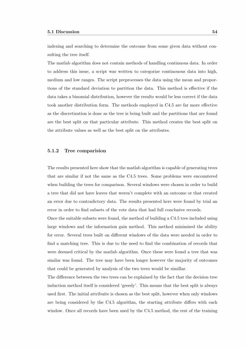
5.1 Discussion 54

indexing and searching to determine the outcome from some given data without con-

sulting the tree itself.

The matlab algorithm does not contain methods of handling continuous data. In order

to address this issue, a script was written to categorize continouous data into high,

medium and low ranges. The script preprocesses the data using the mean and propor-

tions of the standard deviation to partition the data. This method is effective if the

data takes a binomial distribution, however the results would be less correct if the data

took another distribution form. The methods employed in C4.5 are far more effective

as the discretization is done as the tree is being built and the partitions that are found

are the best split on that particular attribute. This method creates the best split on

the attribute values as well as the best split on the attributes.

5.1.2 Tree comparision

The results presented here show that the matlab algorithm is capable of generating trees

that are similar if not the same as the C4.5 trees. Some problems were encountered

when building the trees for comparison. Several windows were chosen in order to build

a tree that did not have leaves that weren’t complete with an outcome or that created

an error due to contradictory data. The results presented here were found by trial an

error in order to find subsets of the vote data that had full conclusive records.

Once the suitable subsets were found, the method of building a C4.5 tree included using

large windows and the information gain method. This method minimised the ability

for error. Several trees built on different windows of the data were needed in order to

find a matching tree. This is due to the need to find the combination of records that

were deemed critical by the matlab algorithm. Once these were found a tree that was

similar was found. The tree may have been longer however the majority of outcomes

that could be generated by analysis of the two trees would be simillar.

The difference between the two trees can be explained by the fact that the decision tree

induction method itself is considered ‘greedy’. This means that the best split is always

used first. The initial attribuite is chosen as the best split, however when only windows

are being considered by the C4.5 algorithm, the starting attribute differs with each

window. Once all records have been used by the C4.5 method, the rest of the training

5.1 Discussion 55

data is then examined in order to find exceptions to the tree. This property means

that attributes may be in the same branch as the matlab tree, however its location in

the tree may vary. This accounts for most of the differences found in the trees.

Other differences can be explained by the choice of initial attribute and the inclusion

of contradictory data. Contradictory data can be dealt with by using pruning methods

as the tree is built. C4.5’s windowing methods use this type of pruning to build trees.

The initial tree is built on a subset of the window, and after this the rules that are

generated are compared with the unused portion of the window, with any contraditions

that prove to be more correct being adapted into the tree. This is an effective method

of adapting to contraditions in the data.

5.1.3 Neural networks

The neural networks method requires some modification of the data structure in order

to employ an effective analysis of the data. This modification includes transforming the

data into a binary form that represents each attribute as a bit. This method creates a

clear distinction between attribute values, thereby removing the ability to have values

that are not clearly represented.

The binary method does create some confusion with the network outputs because these

may be seen to be any combination of numbers if the training of the network is not

entirely correct. The output is very rarely exactly [0 1] or [1 0], therefore a confidence

value was determined in order to simply display a term that would represent the cor-

rectness of the outcome. With this value being employed, it was acceptable to use

rounding methods in order to determine which outcome is actually predicted.

When using particular training and test sets, it was experienced that some of the test

records would produce values such as [-1.02 0.26] which do not correspond to any known

outcome. This output represents the fact that the training set did not contain any sim-

ilar records and the record being tested may have even been contradictory to most of

the training data. In this case an inconclusive result was presented for the record.

The parameters sent to the neural network toolbox created varying results, with con-

vergence rarely being experienced. This is most likely due to the size of the training

set and the fact that the data has been found as a good set for decision tree induction.

5.1 Discussion 56

It has been found that neural networks respond better to training sets that contain a

proportion of noise. These training sets remove the possibility of the network being

restricted to predicting only records that have been in the training set and incorrectly

predicting records that it has not seen before. This property can explain the manner

of predictions that are completely different to any of the desired outcomes.

5.1.4 Method Comparison

When considering categorical data the most powerful method seems to be the decision

tree induction methods because the ‘greediness’ of the algorithms brings the program

to a conclusion much quicker than the networks method. Although the decision tree

methods are very dependant on the training set containing suitable data records, the

networks methods can actually adapt to the data and still create a set of useful weights.

The network method is reliant on the training data being broad enough to cover most of

the examples that are experienced in test/working data set. As a side-note, the matlab

network toolbox contains an adaptive tool that can be used to update the network with

new data when required. This tool re-adjusts the weights of the network. Such a tool

boasts superiority over the decision tree method as a new tree must be built in order

to accomodate changing data.

The trees create an easier to understand method of recording the results of the induc-

tion whereas the networks method is given the record to be examined and no other

knowledge is required. In some instances an understanding of the relations that occur

within the data is required. For example, when examining medical data, it may be

possible to predict when a disease is prevalent with the networks method, however it

is much more useful to examine the decision tree in order to determine the causation

of the disease. The neural network method requires some preprocessing of the data in

order to create a data structure with which it can operate. This data structure incor-

porates an expansion of the amount of data required to represent the attributes. For

example an attribute with three values would be represented by three binary objects

rather than one single string variable.

The neural network method requires a large amount of consideration when training the

network. For example the number of iterations to train the weights for, the number

5.1 Discussion 57

of hidden neurons required and the constants (momentum and learning rate) must be

considered. Decision tree induction does not require these considerations, however this

provides less control over the learning process. In the case of the matlab decision tree

algorithm, the outcome of each record must be a binary variable, for example a pos-

itive or a negative outcome. The neural network method can be used to predict any

number of possible outcomes, in order to create such a network, the number of output

neurons should be increased respective of the number of possible outcomes required.

This adaptability of the method is extremely useful.

The results provided by both methods are acceptable in relation to performance. The

training and test sets used for both methods provided suitable data to compare the

two methods. The high percentage of correct predictions within the test sets illustrates

each method is capable of providing useful results. In the present form the networks

method provides a more accurate portrait of the predictions by giving the confidence

value, however with some modification, a similar method to that used by C4.5 could

be integrated into the algorithm. This method would include recording the informa-

tion gain for each decision and providing the number of records that support over the

number of records that do not support the decision for each leaf of the tree.

5.1.5 Further Work

In order to continue this study, the following areas are worth due attention:

• Pre/Post pruning

The resulting decision trees could be created with much more speed using pre-

pruning. Post pruning can help reduce the size of the final tree by ’pruning’

branches at relevant points in the tree.

• Information feedback

The final tree should include information on the percentage of contradictory data

and pruning points should feedback the percentage of values that opposed the

pruning.

• Contradictory data handling

A method such as C4.5’s windowing method could be adopted in order to lessen

5.1 Discussion 58

the effects of contradictory data. The greater percentage of supporting values

would be chosen as the best split.

• Continuous data handling

A more correct ’on the fly’ method of analysing continuous data should be

adopted. Such as regression tree methods or using the information gain ratio

to find the best continuous split points.

• Graphical user interfaces

Matlabs graphical interfaces are a powerful method in increasing the user freind-

liness of such an algorithm. Selection of the excel spreadsheets files could be

simplified using dialog boxes. All options to parse to the algorithm could be

selected via check boxes and input dialogs.

• Graphical tree representation

The final decision tree could be represented as a visual tree within a matlab figure

dialog thereby heightening the understanding of the programs outputs.

• Toolbox bundling

The final algorithm would be best bundled into toolbox and distributed within a

self installing file.

5.1.6 Implications of the study

This study provided an algorithm for decision tree analysis within the matlab coding

environment. The output of the decision tree was found to be quite similar to that of

the output given by the neural network toolbox that has been implemented for matlab.

An analysis of the effectiveness of the two methods within the matlab language was

conducted. The analysis showed that both implementations are quite effective when

analysing categorical data although the neural network method requires more user

input in order to produce good results.

5.2 Conclusion 59

5.2 Conclusion

Both the neural network and the decision tree induction methods have their merits.

The neural network method is more adaptable, which makes it useful for many sit-

uations. The decision tree method is straightforward and the results are extremely

simple to interpret. Each method provides an avenue for prediction of outcomes based

on sections of data. In each case, the selection of training data is imperative for the

success of the final decisions.

The decision tree induction method lends itself well to implementation within higher

level programming languages such as found in the matlab environment. The environ-

ment provides many tools in which the implementation becomes a simpler process. The

data input methods provided within matlab create an implementation method which

reduces the amount of data preparation required.

When considering categorical data, the matlab implementation of the decision tree in-

duction method provides an equivalent tree to that found by the C4.5 implementation

when no pruning of the tree is involved. Some further implementation is required for

the use of this method in prediction outcomes for continuous data sets. Some prepro-

cessing of the data is required in order to remove the possibility of contradictory data.

Data mining provides a very useful avenue for examining large amounts of data with-

out succumbing to the high cost of processing complete data sets. The neural network

method is a capable data mining method that is highly adaptable. The adapability of

this method is not overshadowed by the higher numbers of incorrect predictions found

in this study. Better results may be found using the matlab decision tree method. This

study resulted in the full implementation of an algorithm to handle categorical data

only. Preliminal implementation of the continuous data handling has been completed

however in this respect, the neural networks method’s results would most likely be more

relevant than any obtained using the decision tree algorithm in its current state.

The case studies evaluated here have little relevance to the current political arena,

however they do serve their purpose as a platform for analysis of the two methods.

References

Blake, C. L. & Merz, C. J. (1998), ‘UCI repository of machine learning databases’.

http://www.ics.uci.edu/∼mlearn/MLRepository.html

Durkin, J. (1991), ‘Designing an induction expert system’, AI Expert December 1991 .

Durkin, J. (1992), ‘Induction...’, AI Expert April 1992 .

Hastie, T., Tibshirani, R. & Friedman, J. (2001), The Elements of Statistical Learning,

Data Mining, Inference, and Prediction, Springer-Verlag, New York, USA.

Krose, B. & van der Smagt, P. (1996), An Introduction to Neural Networks.

Lau, C., ed. (1992), Neural Networks, Theoretical Foundations and Analysis, Institution

of Electrical and Electronic Engineers, Inc, New York.

Mitchell, T. M. (1997), Machine Learning, McGraw Hill, New York.

Quinlan, J. R. (1985), ‘Induction of decision trees’, Centre for Advanced Computing

Sciences .

Quinlan, J. R. (1993), C4.5: Programs for Machine Learning, Morgan Kaufmann Pub-

lishers, Inc, San Mateo CA, USA.

Read, B. J. (2000), ‘Data mining and science?’. Accessed: 23rd March 2004.

http://www.ercim.org/publication/ws-proceedings/12th-EDRG/EDRG12 RE.pdf

Rojas, R. (1996), Neural Networks, A Systematic Approach, Springer-Verlag, Berlin.

Soulie, F. F. & Gallinari, P., eds (1998), Industrial Applications of Neural Networks,

World Scientific Publishing Co., Singapore.

REFERENCES 61

Werbos, P. J. (1990), ‘Backpropagation through time: What it does and how to do it’,

Proceedings of the IEEE .

Widrow, B. & Lehr, M. A. (1990), ‘30 years of adaptive neural networks:perceptron,

madaline and backpropagation’, Proceedings of the IEEE .

Appendix A

Project Specification



ENG 4111/4112 Research Project

PROJECT SPECIFICATION

FOR: Rodney Joseph Woolf

TOPIC: Data Mining Using MATLAB

SUPERVISOR: DR. Sai-Cheong Fok

PROJECT AIM: To enhance and extend the data-mining facilities within

MATLAB using the included toolboxes as well as developing

further data-mining tools.PROGRAMME: Issue A: 22, March 2004

1. Research various data mining techniques and understand the logic behind the

various forms of data analysis and manipulation.

2. Investigate frameworks encompassing the inbuilt and developed modules.

3. Implement and verify selected algorithms and techniques in matlab code.

4. Implement the various modules using clear case studies to evaluate the effectivness

of the system.

5. Develop an user friendly graphical interface for the extended facilities.

As time permits:

6. Develop a help system for the tools.

7. Test the system on various advanced applications for effectiveness.

8. Encompass the tools within an distributable toolbox.

AGREED:

(Student) (Supervisor)

(Dated) / /

Appendix B

Used Data Sets

B.1 Vote data clarification

|

| Voting records drawn from the Congressional Quarterly Almanac, 98th

| Congress, 2nd session 1984, Volume XL: Congressional Quarterly Inc.

| Washington, D.C., 1985.

|

| This data set includes votes for each of the U.S. House of

| Representatives Congressmen on the 16 key votes identified by the

| CQA. The CQA lists nine different types of votes: voted for, paired

| for, and announced for (these three simplified to yea), voted

| against, paired against, and announced against (these three

| simplified to nay), voted present, voted present to avoid conflict

| of interest, and did not vote or otherwise make a position known

| (these three simplified to an unknown disposition).

|

| Jeff Schlimmer, 23 April 1987.

|

democrat,republican | classes

handicapped infants: n, y, u

B.2 Test Data 65

water project cost sharing: n, y, u

adoption of the budget resolution: n, y, u

physician fee freeze: n, y, u

el salvador aid: n, y, u

religious groups in schools: n, y, u

anti satellite test ban: n, y, u

aid to nicaraguan contras: n, y, u

mx missile: n, y, u

immigration: n, y, u

synfuels corporation cutback: n, y, u

education spending: n, y, u

superfund right to sue: n, y, u

crime: n, y, u

duty free exports: n, y, u

export administration act south africa: n, y, u

B.2 Test Data

B.2

.1Test

reco

rds

for

case

study

one

Rec

ord

Att

1A

tt2

Att

3A

tt4

Att

5A

tt6

Att

7A

tt8

Att

9A

tt10

Att

11A

tt12

Att

13A

tt14

Att

15A

tt16

Out

com

e

2y

ny

nn

ny

yu

ny

nn

ny

yde

m

5y

yy

nn

yy

yy

nn

nn

ny

yde

m

9y

yy

nn

ny

yy

ny

un

nn

yde

m

10n

yy

ny

yn

yn

nn

nn

nn

yde

m

11n

yy

nn

yy

yu

ny

yn

ny

yde

m

13n

yy

nn

ny

yn

ny

nn

ny

ude

m

14y

ny

nn

ny

yy

nn

nn

ny

ude

m

18y

yy

nn

ny

yy

nn

nn

nn

yde

m

24y

yy

nn

ny

yy

ny

nn

nn

ude

m

28y

uy

nn

ny

yy

nn

nn

ny

ude

m

23y

yy

ny

yn

yn

ny

ny

ny

yde

m

8n

ny

nn

yy

yy

yn

yn

yy

ude

m

15y

ny

nn

yy

yy

yy

nn

ny

yde

m

16n

yy

nn

yy

yu

yn

nn

nn

yde

m

17y

yy

nn

yy

yy

yn

nn

nn

yde

m

20n

ny

nn

ny

yy

yn

nn

nn

yde

m

25u

ny

nn

ny

yy

yy

un

ny

ude

m

27y

yy

nu

ny

yy

yn

nn

ny

ude

m

6u

uu

nn

ny

yy

yn

ny

ny

yde

m

Tab

leB

.1:

Tes

tda

tafo

rth

efir

stvo

teca

sest

udy

Rec

ord

Att

1A

tt2

Att

3A

tt4

Att

5A

tt6

Att

7A

tt8

Att

9A

tt10

Att

11A

tt12

Att

13A

tt14

Att

15A

tt16

Out

com

e

29y

yy

ny

yn

nn

yy

ny

yn

yde

m

30n

nn

ny

yn

nn

yy

yy

yn

yde

m

21u

uu

un

yn

yy

nn

yy

nn

ure

p

19n

yn

yy

yn

nn

nn

yy

yn

nre

p

22n

nn

yy

yn

nn

nn

yy

yn

yre

p

1n

nn

yy

yy

yy

yn

yy

yn

yre

p

3n

un

yy

yn

nn

yn

yy

yn

yre

p

4n

nn

yy

yn

nn

yu

yy

yn

yre

p

7n

nn

yy

yn

nn

yn

yy

yn

nre

p

12n

un

yy

yn

nn

yn

yy

yn

nre

p

26y

yy

yy

yy

yn

yn

ny

yn

yre

p

Tab

leB

.2:

Rem

aini

ngte

stda

tafo

rfir

stvo

teca

sest

udy

Atr

ribu

tere

fere

nce

Act

ualat

trib

utes

Att

1H

andi

capp

edin

fant

s

Att

2W

ater

proj

ect

cost

shar

ing

Att

3A

dopt

ion

ofth

ebu

dget

reso

luti

on

Att

4P

hysi

cian

fee

free

ze

Att

5E

lsa

lvad

orai

d

Att

6R

elig

ious

grou

psin

scho

ols

Att

7A

ntisa

telli

tete

stba

n

Att

8A

idto

nica

ragu

anco

ntra

s

Att

9M

xm

issi

le

Att

10Im

mig

rati

on

Att

11Sy

nfue

lsco

rpor

atio

ncu

tbac

k

Att

12E

duca

tion

spen

ding

Att

13Su

perf

und

righ

tto

sue

Att

14C

rim

e

Att

15D

uty

free

expo

rts

Att

16E

xpor

tad

min

istr

atio

nac

tso

uth

afri

ca

Tab

leB

.3:

Ref

eren

cela

bels

for

voti

ngat

trib

utes

B.2

.2Test

reco

rds

for

case

study

two

Rec

ord

Att

1A

tt2

Att

3A

tt4

Att

5A

tt6

Att

7A

tt8

Att

9A

tt10

Att

11A

tt12

Att

13A

tt14

Att

15A

tt16

Out

com

e

5y

yy

nn

yy

yy

yn

nn

nn

yde

m

6n

ny

nn

yy

yy

yy

nn

ny

yde

m

7y

yy

nn

ny

yy

nn

nn

ny

yde

m

8n

yy

nn

ny

yy

yn

nu

ny

yde

m

9n

yy

nn

nn

yy

ny

nn

yy

yde

m

10y

ny

nn

ny

yy

yy

ny

ny

yde

m

13y

yy

nn

yy

yy

yy

yy

nn

yde

m

16y

ny

nn

ny

yy

uy

nn

ny

ude

m

17u

uu

uu

uu

uy

uu

uu

uu

ude

m

18n

ny

nn

yy

yy

yn

ny

nn

yde

m

19y

ny

nn

nn

yy

yn

nn

ny

yde

m

20y

yy

nn

yu

yn

ny

yn

yn

ude

m

21y

ny

nn

ny

yn

yy

nn

nn

ude

m

22n

uy

nu

uy

yy

yu

un

ny

yde

m

23n

uy

nn

yn

yn

yy

nn

ny

yde

m

24y

ny

nn

ny

yy

yn

yn

ny

ude

m

25n

nn

ny

yy

nn

nn

yy

yn

yde

m

26n

uy

nn

ny

yy

nn

nn

ny

yde

m

27n

un

nn

yy

yy

yn

nn

yn

ude

m

28n

yy

nn

ny

yy

nn

ny

nu

ude

m

Tab

leB

.4:

Tes

tda

tafo

rth

ese

cond

vote

case

stud

y

Rec

ord

Att

1A

tt2

Att

3A

tt4

Att

5A

tt6

Att

7A

tt8

Att

9A

tt10

Att

11A

tt12

Att

13A

tt14

Att

15A

tt16

Out

com

e

29y

yy

nn

ny

yy

ny

nn

ny

yde

m

30y

ny

nn

ny

yy

yn

nn

ny

ude

m

1n

nn

yy

yn

nn

yn

yy

yn

ure

p

2n

yn

yy

yn

nn

nn

yy

yn

nre

p

3n

yn

yy

yn

nn

nn

ny

yn

yre

p

4n

un

yy

yn

nn

nn

yy

yn

ure

p

11n

nn

yy

yn

nn

yn

yy

yn

nre

p

12n

yn

yy

yn

nn

nn

yy

yn

yre

p

14n

yn

yy

yu

un

yn

yu

uu

ure

p

15n

nn

ny

yy

nn

nn

un

yy

yre

p

Tab

leB

.5:

Rem

aini

ngte

stda

tafo

rse

cond

vote

case

stud

y

Atr

ribu

tere

fere

nce

Act

ualat

trib

utes

Att

1H

andi

capp

edin

fant

s

Att

2W

ater

proj

ect

cost

shar

ing

Att

3A

dopt

ion

ofth

ebu

dget

reso

luti

on

Att

4P

hysi

cian

fee

free

ze

Att

5E

lsa

lvad

orai

d

Att

6R

elig

ious

grou

psin

scho

ols

Att

7A

ntisa

telli

tete

stba

n

Att

8A

idto

nica

ragu

anco

ntra

s

Att

9M

xm

issi

le

Att

10Im

mig

rati

on

Att

11Sy

nfue

lsco

rpor

atio

ncu

tbac

k

Att

12E

duca

tion

spen

ding

Att

13Su

perf

und

righ

tto

sue

Att

14C

rim

e

Att

15D

uty

free

expo

rts

Att

16E

xpor

tad

min

istr

atio

nac

tso

uth

afri

ca

Tab

leB

.6:

Ref

eren

cela

bels

for

voti

ngat

trib

utes

B.3 Training Data 72

B.3 Training Data

B.3.1 Training data for case study one

1,y,y,y,n,n,n,y,y,y,y,y,n,n,n,n,y,dem

2,y,y,y,n,n,n,y,y,y,n,y,n,n,n,y,u,dem

3,y,n,y,n,n,n,y,y,y,n,y,n,n,n,y,u,dem

4,n,n,y,y,y,y,n,n,y,n,n,n,y,y,y,u,dem

5,n,n,n,y,y,y,n,n,n,y,n,y,y,y,n,u,rep

6,n,n,y,y,n,n,y,y,y,y,n,n,n,y,y,y,rep

7,n,y,y,n,n,n,y,y,y,y,y,n,n,n,y,y,dem

8,y,n,n,n,n,y,y,y,y,y,n,n,n,y,y,y,dem

9,n,n,y,n,n,y,y,y,y,y,y,n,n,n,y,y,dem

10,y,n,y,n,y,y,n,n,n,n,n,n,n,n,n,y,dem

11,n,n,y,y,y,y,n,n,y,y,n,y,y,y,n,y,rep

12,n,y,n,y,y,y,n,n,n,y,y,y,y,y,n,n,rep

13,y,n,y,n,n,y,y,y,y,y,y,n,n,n,n,y,dem

14,y,y,y,n,n,n,y,y,u,y,n,n,n,n,y,u,dem

15,n,y,n,y,y,y,n,n,n,n,n,n,u,y,y,y,dem

16,y,u,y,n,n,n,y,y,y,n,n,n,n,n,y,y,dem

17,n,n,y,n,n,n,y,y,y,y,n,n,y,n,y,y,dem

18,y,y,y,u,n,y,y,y,y,n,y,n,y,n,u,y,dem

19,n,y,y,y,y,y,n,n,n,y,n,y,y,y,n,y,rep

20,y,n,y,n,n,n,y,y,n,y,y,n,n,n,n,u,dem

21,n,y,y,n,n,u,y,y,y,y,y,n,u,y,y,y,dem

22,n,y,n,y,y,y,n,n,n,n,n,y,y,y,n,y,rep

23,n,n,y,n,n,n,y,y,y,n,y,n,n,n,y,y,dem

24,y,y,y,n,y,y,y,y,n,y,y,n,n,n,y,u,dem

25,y,u,y,n,n,n,y,y,y,n,y,n,n,n,y,y,dem

26,y,y,n,n,y,y,n,n,n,y,y,y,y,y,n,u,dem

27,y,n,y,n,n,y,n,y,u,y,y,y,u,n,n,y,dem

28,y,n,y,n,n,n,y,y,y,n,n,n,n,n,y,y,dem

29,y,n,n,n,y,y,y,n,n,y,y,n,n,y,n,y,dem

30,y,n,n,y,y,n,y,n,n,y,n,n,n,y,y,y,rep


32,n,y,n,y,y,y,u,u,n,y,n,y,u,u,u,u,rep


33,n,n,n,y,y,y,n,n,n,y,n,y,y,y,y,n,rep

34,n,n,y,n,n,n,y,y,y,n,n,u,n,n,y,y,dem

35,n,n,n,y,y,y,n,n,n,n,n,y,y,y,y,n,rep

36,y,n,y,n,n,n,y,y,y,y,n,n,n,n,y,y,dem

37,n,n,n,y,y,y,n,n,n,y,n,y,y,y,n,y,rep

38,n,n,n,y,y,y,n,n,n,n,n,y,y,y,n,u,rep

39,y,n,y,n,n,y,y,y,n,n,n,y,y,n,n,y,dem

40,y,y,y,n,n,n,y,y,u,n,y,n,n,n,y,u,dem

41,y,y,n,n,y,u,n,n,n,n,y,n,y,y,n,y,dem

42,n,y,n,y,y,y,n,n,n,n,n,y,y,u,n,y,rep

43,n,y,y,n,n,n,y,y,y,y,n,n,u,n,y,y,dem

44,y,y,y,n,n,n,y,y,y,n,n,n,n,n,u,u,dem

45,n,y,y,u,y,y,n,y,n,y,u,n,y,y,u,y,dem

46,y,n,y,n,n,y,y,y,y,n,n,y,u,y,y,y,dem

47,y,n,y,n,n,n,y,y,y,n,n,n,n,n,y,u,dem

48,y,y,y,n,n,y,y,y,u,y,y,u,n,n,y,u,dem

49,y,n,y,n,n,n,y,y,y,y,y,n,y,n,y,y,dem

50,n,n,y,n,n,n,y,y,y,n,n,n,n,y,y,y,dem

51,n,n,n,y,y,y,n,n,n,n,n,y,y,y,n,n,rep

52,y,y,y,n,n,n,y,y,y,n,y,n,n,n,y,y,dem

53,n,n,n,y,y,y,y,n,n,y,n,y,y,y,n,y,rep

54,y,u,n,y,y,y,n,y,n,n,n,y,y,y,n,y,rep


56,y,y,y,n,y,y,n,y,u,y,n,n,y,y,n,u,dem

57,n,u,y,n,n,n,y,y,y,n,n,n,n,n,y,y,dem

58,n,u,y,n,n,n,y,y,y,y,y,n,n,y,y,y,dem

59,y,y,u,u,u,y,n,n,n,n,y,n,y,n,n,y,dem

60,n,n,y,n,n,n,y,y,y,y,y,u,n,n,y,y,dem

61,n,y,n,y,y,y,n,u,n,y,n,y,y,y,n,u,rep

62,n,u,y,n,n,y,y,y,y,y,n,n,n,y,y,y,dem

63,n,y,n,y,y,y,n,n,n,n,n,u,y,y,n,n,rep


65,y,n,y,y,y,n,y,n,y,y,n,n,y,y,n,y,rep

66,n,u,y,n,y,y,n,y,n,n,y,n,n,n,n,u,dem

67,y,n,y,n,n,n,y,y,y,u,y,n,n,n,y,u,dem

68,y,y,n,y,y,y,n,n,n,y,n,y,y,y,n,y,rep

69,n,u,y,n,u,u,y,y,y,y,u,u,n,n,y,y,dem


70,n,y,y,n,n,y,y,y,y,y,n,u,n,n,y,y,dem

71,y,y,n,y,y,y,n,u,n,n,y,y,y,y,n,n,rep

72,y,n,y,n,n,n,y,y,y,y,n,n,n,n,n,y,dem

73,y,n,y,n,u,n,y,y,y,y,n,y,n,u,y,y,dem

74,n,y,y,n,y,y,n,n,n,y,y,y,y,y,n,u,dem


76,n,n,n,y,n,n,y,y,y,y,n,n,y,y,n,y,rep

77,y,y,n,y,y,y,n,n,n,n,n,n,y,y,n,y,rep


79,n,n,y,y,y,y,y,n,n,n,n,y,y,y,n,y,rep

80,y,n,y,n,n,y,y,y,y,y,n,y,n,y,n,u,dem

81,n,y,y,y,y,y,y,u,n,n,n,n,u,u,y,u,rep

82,y,u,n,y,y,y,y,n,n,y,n,y,y,y,n,y,rep

83,n,n,n,n,y,y,y,n,n,n,n,y,y,y,n,y,dem

84,u,u,u,u,u,u,u,u,u,u,u,u,u,u,u,u,rep

85,n,y,n,y,y,y,n,n,n,n,y,y,n,y,n,n,dem

86,y,y,n,y,y,y,n,n,n,n,y,n,y,y,n,y,rep

87,y,y,n,y,y,y,n,n,n,y,n,y,y,y,n,y,rep

88,y,y,y,n,n,n,y,y,y,y,n,n,y,n,n,y,dem

89,y,n,y,n,n,y,y,y,n,y,y,n,y,y,y,y,dem

90,n,n,y,y,y,y,y,y,n,y,n,n,n,y,n,y,rep

Note: The columns are arranged in the same order as that of the test data

B.3.2 Training data for case study two

1,y,n,y,n,n,y,y,y,y,y,y,n,n,n,y,y,dem

2,n,y,n,y,y,y,n,n,n,n,n,y,y,y,n,n,rep

3,n,u,y,y,y,y,n,n,n,y,n,n,n,y,n,y,rep

4,y,y,n,y,y,y,n,n,n,n,y,y,y,y,n,y,rep


6,y,u,y,n,n,n,y,y,y,n,u,n,n,n,y,u,dem

7,n,n,n,y,y,y,n,n,n,n,n,y,y,y,n,y,rep


9,n,u,n,y,y,y,n,n,n,n,n,y,y,y,n,n,rep

10,y,y,y,n,n,n,y,y,u,y,n,n,n,n,y,u,dem


11,n,u,y,n,y,y,n,y,n,n,y,n,n,n,n,u,dem

12,n,n,n,y,y,y,n,n,n,y,n,y,n,y,n,y,rep

13,y,n,y,n,n,n,y,y,y,n,n,n,n,n,y,u,dem

14,y,n,y,n,n,y,y,y,y,n,n,n,n,n,y,y,dem

15,n,n,n,y,y,y,y,y,y,y,n,y,y,y,n,y,rep


17,n,y,y,n,n,n,y,y,y,y,n,n,n,n,y,y,dem

18,y,y,n,n,y,u,n,n,n,n,y,n,y,y,n,y,dem


20,n,y,n,y,y,y,n,n,n,n,n,u,y,y,n,n,rep

21,n,y,n,y,u,y,n,n,n,y,n,y,y,y,n,n,rep

22,n,n,n,y,y,y,n,n,n,n,n,y,y,y,n,y,rep

23,n,y,n,y,y,y,n,n,n,y,n,u,y,y,n,n,rep

24,y,n,y,n,n,n,y,y,y,n,n,n,n,n,u,y,dem

25,n,y,y,n,n,y,y,y,y,y,n,n,y,y,y,y,dem

26,n,n,n,y,y,y,n,n,n,n,n,y,y,y,n,u,rep

27,n,u,y,n,n,y,y,y,y,y,n,n,n,y,y,y,dem

28,y,y,y,n,y,y,n,y,u,y,n,n,y,y,n,u,dem

29,n,n,y,n,n,y,y,y,n,n,y,n,n,y,u,y,dem

30,n,y,n,y,y,y,n,n,n,n,n,y,y,u,n,y,rep

31,y,y,u,u,u,y,n,n,n,n,y,n,y,n,n,y,dem

32,y,u,y,n,n,n,y,y,y,n,n,n,n,n,y,u,dem

33,n,n,n,y,y,y,y,y,y,y,n,y,y,y,u,y,rep


35,y,y,n,y,y,y,n,n,n,n,n,n,y,y,n,y,rep

36,y,u,n,y,y,y,y,y,n,n,n,y,u,y,u,u,rep

37,n,y,y,n,n,y,y,y,y,n,u,n,n,n,n,y,dem

38,y,n,y,n,n,y,y,y,n,y,y,n,y,y,y,y,dem

39,y,y,n,y,y,y,y,n,n,n,n,y,y,y,n,y,rep

40,y,u,n,y,y,y,y,n,n,y,n,y,y,y,n,y,rep

41,n,y,y,n,n,y,y,y,y,n,y,n,n,y,y,y,dem

42,y,n,y,n,n,n,y,y,y,n,y,n,n,n,y,u,dem

43,n,y,y,u,y,y,n,y,n,y,u,n,y,y,u,y,dem

44,y,y,y,u,n,y,y,y,y,n,y,n,y,n,u,y,dem


46,n,n,n,n,n,n,y,y,y,y,n,y,y,y,y,y,dem

47,n,u,y,n,n,y,y,y,n,y,n,n,n,n,y,u,dem


48,y,y,n,n,n,n,n,y,y,n,y,n,n,n,y,n,dem

49,n,y,n,n,n,n,y,y,y,y,y,n,n,n,y,y,dem

50,y,y,y,n,y,y,n,n,n,n,y,u,y,y,y,y,dem

51,n,n,n,y,y,y,n,n,n,y,n,y,y,y,n,n,rep

52,n,y,n,y,y,y,n,n,n,n,y,u,y,y,u,u,rep

53,y,n,y,n,n,y,y,y,y,y,n,y,n,y,n,u,dem

54,y,n,y,n,n,n,y,y,y,y,n,n,n,n,n,y,dem

55,y,y,y,n,y,y,n,y,y,y,y,n,n,n,n,y,dem

56,y,n,y,n,n,y,y,y,n,n,n,y,y,n,n,y,dem

57,y,n,n,y,y,n,y,n,n,y,n,n,n,y,y,y,rep

58,n,y,n,y,y,y,n,n,n,y,n,y,y,u,n,u,rep


60,y,u,y,n,n,n,y,y,y,n,n,n,n,n,y,y,dem

61,n,y,y,y,y,y,n,n,n,y,y,y,y,y,y,u,dem

62,n,y,n,y,y,y,n,n,n,n,n,y,u,u,n,u,rep

63,n,y,n,y,y,y,y,n,n,n,n,y,y,y,n,y,rep

64,y,y,n,y,y,y,y,n,n,n,n,y,y,y,n,n,rep

65,y,y,y,n,n,n,y,y,y,n,y,n,n,n,n,u,dem

66,n,u,n,y,y,y,n,n,n,y,n,y,y,y,n,n,rep

67,n,n,y,y,y,y,n,n,y,y,n,y,y,y,n,y,rep


69,y,y,u,y,y,y,n,n,y,n,y,u,y,y,n,n,dem

70,n,y,n,y,y,y,n,n,n,n,n,n,u,y,y,y,dem


72,n,n,y,n,n,n,y,y,y,n,n,n,n,y,y,y,dem

73,n,n,y,y,y,y,y,y,n,y,n,n,n,y,n,y,rep

74,y,y,y,n,n,n,y,y,y,n,n,n,u,u,y,y,dem

75,y,n,y,n,n,n,y,y,y,y,n,n,u,n,y,y,dem

76,y,n,y,n,y,y,n,n,n,n,n,n,n,n,n,y,dem

77,n,n,n,y,y,n,y,n,y,y,n,n,n,y,n,y,rep

78,y,y,y,y,y,y,y,y,n,y,u,u,u,y,n,y,rep

79,y,y,y,n,n,n,n,y,y,n,y,n,n,n,y,y,dem

80,n,n,y,y,y,y,n,n,y,n,n,n,y,y,y,u,dem

81,n,y,y,n,y,y,y,n,y,y,y,n,y,y,n,y,dem

82,y,n,n,y,y,y,n,n,n,n,y,y,y,y,n,n,rep

83,y,y,y,n,n,n,y,y,y,n,n,n,n,n,y,y,dem

84,y,y,y,n,n,n,y,y,y,n,n,n,n,n,y,y,dem



86,n,n,y,n,n,n,y,y,y,y,y,n,n,n,y,y,dem

87,n,n,y,n,n,n,y,y,y,y,n,n,y,n,y,y,dem

88,y,y,n,y,y,y,n,n,n,y,n,n,y,y,n,y,rep


90,n,n,y,y,y,y,y,n,n,n,n,y,y,y,n,y,rep

Note: The columns are aligned in the same order as in the test data

Appendix C

Tree Outputs

Decision tree for the first case study of the voting data, found using Matlab

Tree Level 1 branch 1

>> physician fee freeze

-> n

dem

-> y

>>>>

-> u

>>>>


>> immigration

-> n

>>>>

-> y

rep

-> u

rep

APPENDIX C. TREE OUTPUTS 79


>> superfund right to sue

-> n

dem

-> y

>>>>

-> u

>>>>


>> mx missile

-> n

rep

-> y

dem

-> u

rep


>> adoption of the budget resolution

-> n

dem

-> y

rep

-> u

dem


>> handicapped infants


-> n

dem

-> y

dem

-> u

rep

Decision tree for the first case study, built by C4.5

Decision Tree:

physician fee freeze = n: dem (13.0)

physician fee freeze = y:

| immigration = y: rep (13.0)

| immigration = u: rep (0.0)

| immigration = n:

| | superfund right to sue = n: dem (1.0)

| | superfund right to sue = y: rep (8.0/1.0)

| | superfund right to sue = u: dem (2.0/1.0)

physician fee freeze = u:

| handicapped infants = n: dem (1.0)

| handicapped infants = y: dem (2.0)

| handicapped infants = u: rep (2.0)

Matlab generated decision tree for the second case study of the voting data


>> physician fee freeze

-> n

dem

-> y

>>>>

-> u

dem



>> duty free exports

-> n

>>>>

-> y

>>>>

-> u

rep


>> adoption of the budget resolution

-> n

rep

-> y

rep

-> u

dem


>> handicapped infants

-> n

dem

-> y

rep

-> u

dem


C4.5 decision tree for second voting case study

Decision Tree:

physician fee freeze = n: dem (14.0/1.0)

physician fee freeze = u: dem (3.0)

physician fee freeze = y:

| duty free exports = y: dem (3.0/1.0)

| duty free exports = u: rep (2.0)

| duty free exports = n:

| | adoption of the budget resolution = n: rep (8.0)

| | adoption of the budget resolution = y: rep (2.0)

| | adoption of the budget resolution = u: dem (1.0)

Appendix D

Neural Network outputs

D.1 Golf script and outputs

test data =

1 1 0 0 0 0 0 1 1 0 1 0 0 0

0 0 1 0 0 0 1 0 0 0 0 1 1 0

0 0 0 1 1 1 0 0 0 1 0 0 0 1

1 1 1 0 0 0 0 0 0 0 0 0 1 0

0 0 0 1 0 0 0 1 0 1 1 1 0 1

0 0 0 0 1 1 1 0 1 0 0 0 0 0

1 1 1 1 0 0 0 1 0 0 0 1 0 1

0 0 0 0 1 1 1 0 1 1 1 0 1 0

1 0 1 1 1 0 0 1 1 1 0 0 1 0

0 1 0 0 0 1 1 0 0 0 1 1 0 1

test outcomes =

0 0 1 1 1 0 1 0 1 1 1 1 1 0

1 1 0 0 0 1 0 1 0 0 0 0 0 1

D.1 Golf script and outputs 84

% Testing the network % % Decision Tree via ID3 % Outlook % —- Overcast -¿ Play

% —- Sunny — % — — Humidity % — —-High -¿ Don’t Play % — —-Normal -¿ Play

% —- Rain — % — Wind % —-Strong -¿ Don’t Play % —-Weak -¿ Play % % Input

data is: % Sunny, Hot, High, Weak. % = Dont’Play echo off

outcome =

Dont Play

% Overcast, Mild, High, Weak.

% = Play

echo off

outcome =

Play

% Rain, Cool, High, Weak

% = Play

echo off

outcome =

Play

% Rain, Mild, Normal, Strong

% = Don’t Play

echo off

outcome =

Play


% Sunny, Hot, Normal, Strong

% = Play

echo off

outcome =

Play

% Overcast, Mild, Normal, Weak

% = Play

echo off

outcome =

Play

record =

1

outcome =

Dont Play

outcome =

Dont Play

record =

2

outcome =

Dont Play


outcome =

Dont Play

record =

3

outcome =

Play

outcome =

Play

record =

4

outcome =

Play

outcome =

Play

record =

5

outcome =

Play

outcome =

Play


record =

6

outcome =

Dont Play

outcome =

Dont Play

record =

7

outcome =

Play

outcome =

Play

record =

8

outcome =

Dont Play

outcome =

Dont Play

record =

9


outcome =

Play

outcome =

Play

record =

10

outcome =

Play

outcome =

Play

record =

11

outcome =

Play

outcome =

Play

record =

12

outcome =

Play


outcome =

Play

record =

13

outcome =

Play

outcome =

Play

record =

14

outcome =

Dont Play

outcome =

Dont Play

Appendix E

Program Listings

E.1 C4.5 algorithm

E.1.1 start.m

%file name=’golf ’;

%pos outcome=’yes’;

%neg outcome=’no’;

file name='vote_used_2';

pos outcome='dem';

neg outcome='rep';

% file name=’votewind’;

% pos outcome=’democrat’; 10

% neg outcome=’republican’;

% file name=’mush’;

% pos outcome=’e’;

% neg outcome=’p’;

% file name=’mush’;

% pos outcome=’e’;

% neg outcome=’p’;

20

E.1 C4.5 algorithm 91

buildtree(file name,pos outcome,neg outcome,75,0);

E.1.2 buildtree.m

function [ ] = buildtree(file name,pos outcome,neg outcome,percent to train,precision threshold)

% % Written by R Woolf, q10222583

% % University of Southern Queensland, Australia

% % Accompanying ID3 algorithm

% %

% %

% %———————————–%

% %—– Decision Tree Algorithm —–%

% %- Based on Quinlans C4.5 and ID3 –%

% %— Written by Rodney Woolf 2004 –% 10

% %———————————–%

% %

% %

% % Limitations

% % ∗ This algorithm does not handle data which is contradictory.

% % A solution to this problem is to use a training window small enough to exclude

% % all contradictory terms, this may require several runs in order to randomly choose

% % such a set.

% % ∗ This algorithm as yet is not suitable for continuous data.

% % In order to overcome this problem, a seperate discretisation algorithm is provided. 20

% %

% %

% % How to call this function

% % buildtree(file name,pos outcome,neg outcome)

% % eg buildtree(’golf ’,’yes’,’no’)

% %

% %

% % Basic steps of the algorithm

% %

% % 30

% % Create a root node for the tree

% %

% % if all leaves of the tree are positive, return a positive identifier (+)

% % if all leaves of the tree are negative, return a negative identifier (-)


% %

% % else

% %

% % for each attribute value, find the next best value for information gain

% % then use this value to recursively find the next best attribute value

% % until all valuess lead to a result (ie 100% positive or negative) 40

% %

% % then return the information in an understandable tree form.

% %

% %

% %

% % Input/Output Files:

% %

% % Input files:

% % Filename.xls

% % Filename.types.xls 50

% %

% % Output Files:

% % Filename.tree - The decision tree - explanation given later

% % Filename.set - Listing of the sets and subsets used in building the tree

% % Filename train.dat - Portion of data used to build the tree

% % Filename test.dat - Portion of the data left for testing purposes

% %

% % Input Variables:

% %

% % file name = The prefix of the data files, eg file name = ’golf ’, for golf.xls and golf.types.xls 60

% % pos outcome = The outcome that will be considered a positive outcome, eg pos outcome= ’yes’

% % if the outcomes are binary ie 1/0 then pos outcome = 1

% % neg outcome = The negative outcome, as above

% % precision threshold = The threshold for deciding what proportion of the data will be considered

% % 100% one attribute value. ie the information gain should be less than this for an

% % attribute to be chosen as the best attribute

% % percent to train = The percentage of the data that will be used to build the tree

% %

% %

% % 70

% % Tree structure

% %

% % An example of the decision tree file golf.tree is given below.

% %


% % Tree Level 1 branch 1

% %

% % >> outlook

% % -> sunny

% % >>>>

% % -> overcast 80

% % yes

% %

% % -> rain

% % >>>>

% %


% %

% % >> humidity

% % -> high

% % no 90

% %

% % -> normal

% % yes

% %

% %


% %

% % >> wind

% % -> weak

% % yes 100

% %

% % -> strong

% % no

% %

% %

% %

% % Interpreting the trees:

% % ∗ An attribute is identified by ’>>’

% % and its values by ’->’

% % ∗ If an outcome is present for this attribute value, it will be seen 110

% % below the value, otherwise a ’>>>>’ is present.

% % ∗ A ’>>>>’ means that the tree moves on to another branch/level

% % ∗ The Tree Level is given as the tree progresses, and a branch number is given.

% %


% % ∗ The root attribute will be the first attribute.

% % The next attribute corresponds to the topmost branch in the root attribute

% % eg For the attribute Outlook, the value sunny has no outcome, this is branch 1 therefore

% % the next level of the tree will begin with the attribute humidity.

% % The value overcast has an outcome of yes, therefore no branch is required.

% % Obviously rain branches to the attribute wind. 120

% %

% % ∗ The tree will therefore be:

% % Outlook

% % / | \

% % / | \

% % Sunny / | \ Rain

% % / | \

% % / |Overcast\

% % / | \

% % Humidity Yes Wind 130

% % / \ / \

% % High / \ Normal Weak / \ Strong

% % / \ / \

% % No Yes Yes No

% %

% %

% %

% % Program/Function listing

% % buildtree.m

% % id3.m 140

% % getdata.m

% % gettypes.m

% % getvalues.m

% % choose set.m

% % create ref point.m

% % build subsets.m

% % find entropy.m

% % find entropy numerical.m

% % save data.m

% % remove missing data.m 150

% % write set.m

% % remove attributes.m

% %

% %


set(0, 'RecursionLimit', 500)

%% Set the recursion limit for debugging purposes

%% ———————————

%% Initialise Variables 160

examples start={};

store k =[ ];

tree level=0;

target attribute=[ ];

record target=[ ];

examples index=[ ];

%% ———————————/

170

%% Set a precision threshold for the information gain default:0

echo

% Loading data, Please wait . . .

echo

tic

a=getdata(file name);

%% Call function to input training and test data from an XLS worksheet 180

toc

store a=a;

index=randperm(length(store a));

%% select random indexes for the order of the attribute values

train window=round(percent to train / 100 ∗ length(store a));

%% Set the percentage of the initial set in order to build the

%% training and test sets

190

a=store a(index(1:train window),:);

%% Select the training set

train data = a;

%% Record training set for output to file


test data = store a(index(train window+1:length(store a)),:);

echo

% Loading attributes and values . . .

echo 200

tic

attributes start=gettypes(file name)'; %% Extract the attributes to be examined

attribute values start=getvalues(file name); %% Extract the attribute values to be examined

toc

a1=size(a); %% Find dimensions of the data

b1=a1(1);

c1=a1(2);

210

a=sortrows(a,c1); %% Sort the data according to the outcome

outcome array=a(:,c1); %% Save the outcomes as a seperate var

for i=1:c1−1

examples start=[examples start a(:,i)]; %% Save the examples as a seperate var

end

%% /———————————

%% Build a binary outcome set 220

%% Replace a positive outcome with 1

%% Replace a negative outcome with 0

%%

if iscellstr(outcome array)==1 %% Test for string outcomes, otherwise

for i=1:b1;

if strcmp(outcome array(i),pos outcome) == 0; %% assume binary type data

y(i) = 0;

elseif strcmp(outcome array(i),neg outcome) == 0;

y(i) = 1;

end 230

end

outcomes start=y';

else

outcomes start=outcome array;


end

%% ———————————/

%% /———————————

%% Initialise other var’s 240

examples now=examples start;

outcomes now=outcomes start;

attributes orig=attributes start;

attributes now = attributes start;

examples orig=examples start;

examples locations=[b1 c1]';

last examples=examples start;

first run=1;

outcomes orig = outcomes start; 250

%% ———————————/

%% /———————————

%% Initialise file for output

file ext='.tree';

output file=strcat(file name,file ext);

file ext='.set';

examples file=strcat(file name,file ext); 260

file id=fopen(output file,'wt');

set file id=fopen(examples file,'wt');

%% ———————————/

if iscellstr(attribute values start) %% Find data type 1 for string, 0 for numerical

data type=1;

else 270

data type=0;

end

save data(file name,train data,data type,0); %% Save the training data to a file for extraction


save data(file name,test data,data type,1); %% Save the testing data to a file for extraction

clear test data train data; %% Clear un-needed variables

%% Replace missing attribute values with the most

%% common value for that attribute 280

echo

% Removing missing data

echo

[examples start] = remove missing data(examples start,outcomes start,attribute values start);

echo

% Starting to build tree, Please wait . . .

echo 290

tic

%% /———————————

%% Call the recursive tree building

%% algorithm -> id3()

[attributes, target attribute, examples,outcomes,record target,store k] = id3(pos outcome,neg outcome,

attribute values start,target attribute, examples start,outcomes start,attributes start,examples orig,

examples index,examples locations,first run,outcomes orig,record target,precision threshold,examples now,

outcomes now,file id,data type,set file id,store k,attributes now,last examples,tree level); 300

%% ———————————/

status=fclose('all'); %% Close files now that writing is finished

toc

E.1.3 getdata.m

function [a]=getdata(file name)

%% Written by R Woolf, q10222583

%% University of Southern Queensland, Australia

%% Accompanying ID3 algorithm

%%


%%

%% This function grabs the exdample data and outcome data

%% from file name.xls

%% Called by buildtree.m

file ext='.xls'; 10

input file=strcat(file name,file ext);

input file=char(input file)

[aa a]=xlsread(input file);

if isempty(a)

a= aa;

end

E.1.4 gettypes.m

function [b]=gettypes(file name)




%%

%%

%% This function grabs the attributes from file name.types.xls


%%

file ext='.types.xls'; 10


input file=char(input file);

[aa file] = xlsread(input file);

k=length(file);

for i= 1:k

b(i) = file(i);

end

20

E.1.5 getvalues.m

function [c]=getvalues(file name)





%%

%%

%% This function grabs the attribute values from file name.types.xls


%%

file ext='.types.xls'; 10


input file=char(input file);

[aa file]=xlsread(input file);

k=size(file);

l=k(2);

k=k(1);

if isempty(aa)

for i=1:k

for j=2:l 20

if iscellstr(file(i,j))==0

c(i,j−1)={'void'};

else

c(i,j−1) = file(i,j);

end

end

end

else

for i=1:k

for j=2:l 30

if isreal(aa(i,j−1))==0

c(i,j−1)=[12345];

else

c(i,j−1) = aa(i,j−1);

end

end

end

end


E.1.6 save data.m

function [ ]=save data(file name,test data,data type,flag)




%%

%%

%% This function is used to output the test and training sets to

%% their respective files


%% 10

file ext='.dat';

if flag == 1

file name=strcat(file name,'_test');

elseif flag == 0

file name=strcat(file name,'_train');

end

file name=strcat(file name,file ext); 20

file name=char(file name);

file id=fopen(file name,'wt');

size test data=size(test data);

for j=1:size test data(1)

for i=1:size test data(2)

if data type==1

write object=char(test data(j,i));

fprintf(file id,'%10s',write object');

end 30

if data type==0

write object=test data(j,i);

fprintf(file id,'%10d',write object');

end

end

fprintf(file id,'\n');

end

status=fclose(file id);


E.1.7 id3.m

function [attributes, target attribute, examples,outcomes,record target,store k] = id3(pos outcome,neg outcome,

attribute values,target attribute, examples,outcomes,attributes,examples orig,examples index,examples locations,

first run,outcomes orig,record target,precision threshold,examples now,outcomes now,file id,data type,set file id,

store k,attributes now,last examples,tree level)




%%

%%

%% ID3.m 10

%% The main recursive algorithm called by buildtree.m and id3.m

%% This function chooses the best attribute via entropy, if the

%% attribute has outcomes for each value then the algorithm exits.

%% Otherwise the algorithm builds subsets that contain each of

%% this attributes values and returns these subsets to itself

%% recursively.

%%

%% An example of how to call this function is found in buildtree.m,

%% however buildtree.m will format the data correctly for use with

%% id3.m. 20

%% It is not suggested call id3.m directly

%%

%% —————- Initialisation ——————

minent record=[ ];

first attrib=1;

branch={'branch'}; % branch identifier in tree

no outcome={' No outcome - Most probably conflict in data '};

attribute values now=attribute values;

outcomes now=outcomes; 30

examples now=examples;

%% —————————————

% return if all outcomes are the same


tree level=tree level+1;

%% increment the tree level in order to aid determination of the tree in file name.tree

40

if first run==1

examples locations=[length(examples)+1]; %% Set the initial index of the set

length index = length(examples locations);

else

examples locations=find(outcomes now==10); %% Set indexes for each subset of examples

length index = length(examples locations)−1;

end

for k=1:length index %% for each set find the best split 50

if isempty(examples locations) %% exit if no data present

errordlg('examples_locations empty');

fclose('all')

return

end

if isempty(examples now)

errordlg('no more examples');

fclose('all') 60

return

end

if first run˜=1

%% Remove the last used subset

examples now=examples now(examples locations(1)+1:length(examples now),:);

outcomes now=outcomes now(examples locations(1)+1:length(outcomes now));

examples locations=find(outcomes now==10);

end

70

%% Create a node for referencing

%% ————- Discrete attributes

if data type==1

corresponding values={'node'};

end

%% —————— Numerical attributes


if data type==0

corresponding values=[12345];

end

80

this index=find(strcmp(target attribute,attributes now)==0);

%% Find the index to remove the attributes that have been used in the tree

if first run˜=1

attributes now=attributes now(this index);

examples now=examples now(:,this index); %% Remove the examples that are the used attribute values

end

if isempty(examples) %% Exit if no data present 90

return

end

%% —————— Choose the current set for the attribute value being examined ——————–

[examples,outcomes,attributes] = choose set(examples,examples now,examples locations,attributes,outcomes,

outcomes now,first run,k,target attribute,first attrib,this index);

100

%% —————— Output the decision tree and current data set to their respective files ——————–

write set(examples,outcomes,set file id,data type);

%% —————————————

% return if attributes array is empty

if isempty(attributes)==1

no outcome=char(no outcome); 110

%% If there are no more attributes left to build the tree output an error and exit

fprintf(file id,'%s',no outcome);

return

end

%% ——————- Find the entropy for each value and attribute in the current set ——————–


%% ————- Discrete attributes

if data type==1

[minent,entrop,corresponding values,entropi] = find entropy(examples,attribute values,outcomes, 120

corresponding values);

end

%% —————— Numerical attributes

if data type==0

[minent,entrop,corresponding values,entropi] = find entropy numerical(examples,attribute values,outcomes,

corresponding values);

end

%% Find the best attribute from attributes 130

current attribute=attributes(minent);

target attribute=attributes(minent);

%% Add next reference point

if data type==1

node index=find(strcmp(corresponding values,'node'));

end

if data type==0

node index=find(corresponding values==12345); 140

end

fprintf(file id,' Tree_Level %d branch %d \n\n',tree level,k);

%% Output the current attribute to the data file

write attribute=char(current attribute);

fprintf(file id,'>> %s \n',write attribute);

%% ——————– Build the next lot of subsets that correspond to the current value ———————–

150

[line end] = create ref point(data type,examples); %% Create correctly dimensioned reference point

%% Build subsets for each value of the best attribute

[examples,outcomes] = build subsets(examples,outcomes,branch,pos outcome,neg outcome,minent,node index,

corresponding values,entrop,line end,precision threshold,file id,data type,tree level);


%% Record the used attributes for removal

minent record = [minent record minent];

record target=[record target target attribute];

160

%% Remove the used attributes

[attributes,attribute values] = remove attributes(minent record,attributes,attributes now,attribute values);

attributes low=attributes(1:minent record−1);

attributes high=attributes(minent record+1:length(attributes));

attributes this run=[attributes low; attributes high];

%% Reset flag

first attrib=0;

first run=first run+1; 170

%% Recurr the algorithm in order to build the tree

[attributes, target attribute, examples,outcomes,record target,store k] = id3(pos outcome,neg outcome,

attribute values,target attribute,examples,outcomes,attributes this run,examples orig,examples index,

examples locations,first run,outcomes orig,record target,precision threshold,examples now,outcomes now,

file id,data type,set file id,store k,attributes now,last examples,tree level);

end

E.1.8 choose set.m

function [examples,outcomes,attributes] = choose set(examples,examples now,examples locations,attributes,outcomes,

outcomes now,first run,k,target attribute,first attrib,this index)




%%

%%

%% This function chooses the set for which the best attribute will

%% be found in this instance

%% If it is the first run of the algorithm, the entire set is chosen 10

%% Otherwise the first set in the examples set is chosen

%% ie up to the first ’eor’ index

if first run==1

examples=examples now;


outcomes=outcomes now;

if isempty(target attribute)==0

examples=examples(:,this index);

end

else

examples=examples now(1:examples locations(1)−1,:); 20

outcomes=outcomes now(1:examples locations(1)−1);

end

E.1.9 write set.m

function [ ] = write set(examples,outcomes,set file id,data type)




%%

%%

%% This function is used to output the subsets to a file

%% for verification purposes


10

size examples=size(examples);

for j=1:size examples(1)

for i=1:size examples(2)

if data type==1

write object=char(examples(j,i));

fprintf(set file id,'%10s',write object');

end

if data type==0

write object=examples(j,i); 20

fprintf(set file id,'%10d',write object');

end

end

write object=outcomes(j);

fprintf(set file id,'%2d',write object');

fprintf(set file id,'\n');

end


fprintf(set file id,'\n');

E.1.10 find entropy.m

function [minent,entrop,corresponding values,entropi] = find entropy(examples,attribute values,outcomes,

corresponding values)




%%

%%

a=size(examples); % determine size of data 10

b=a(1); % number of records

c=a(2); % number of attributes

d=size(attribute values);

inst =[ ];

pr =[ ];

index6=1;

for i=1:d(1)

for j=1:d(2) 20

if strcmp(attribute values(i,j),'void')==0

if i <= a(2)

corresponding values = [corresponding values attribute values(i,j)];

[inst i, inst j, inst k] = find(strcmp(attribute values(i,j),examples(:,i))==1);

if isempty(inst i)

prob = 2;

inst = [inst 1];

else

inst=[inst sum(strcmp(attribute values(i,j),examples(:,i))==1)]; 30

prob=length(find(outcomes(inst i)==1));

end

pr=[pr prob];

end

end


end

corresponding values = [corresponding values {'node'}];

end

% determine probability 40

index1 = find(inst==0);

inst(index1)=1e−12;

probpos = pr./inst;

probneg = 1−probpos;

% if 0 values are present, replace them with 1e-12 as log(0) results in overflow

index1 = find(probpos==0); 50

index2 = find(probneg==0);

probpos(index1)=1e−12;

probneg(index2)=1e−12;

phi = (−probpos.∗log2(probpos))−(probneg.∗log2(probneg));

entrop = 1/b∗(inst.∗phi);

% fix the replacing that occurred above 60

index3=find(entrop<1e−10);

entrop(index3)=0;

entropi=[ ];

for i = 1:d(1)

if i <= a(2)

index5 = sum(strcmp(attribute values(i,:),'void')==0);

entropi=[entropi sum(entrop(index6:index5+index6−1))];

index6=index6+index5;

end 70

end

% ——————————————————————- %

minent = min(entropi);


minent = find(minent==entropi);

% select first occurence if more than one exists

80

if isempty(minent)==1

errordlg('Could not calculate entropy values','Error')

return

end

if length(minent)˜=1

minent=minent(1);

end

E.1.11 find entropy numerical.m

function [minent,entrop,corresponding values,entropi] = find entropy numerical(examples,attribute values,outcomes,

corresponding values)




%%

%%

a=size(examples); % determine size of data 10

b=a(1); % number of records

c=a(2); % number of attributes

d=size(attribute values);

inst =[ ];

pr =[ ];

index6=1;

for i=1:d(1)

for j=1:d(2)

if isnan(attribute values(i,j))==0 20

if i <= a(2)

corresponding values = [corresponding values attribute values(i,j)];


[inst i, inst j, inst k] = find(attribute values(i,j)==examples(:,i));

inst=[inst sum(attribute values(i,j)==examples(:,i))];

prob=length(find(outcomes(inst i)==1));

pr=[pr prob];

end

end

end 30

corresponding values = [corresponding values 12345];

end

% determine probability

index1 = find(inst==0);

inst(index1)=1e−12;

probpos = pr./inst;

probneg = 1−probpos; 40

% if 0 values are present, replace them with 1e-12 as log(0) results in overflow

index1 = find(probpos==0);

index2 = find(probneg==0);

probpos(index1)=1e−12;

probneg(index2)=1e−12;

phi = (−probpos.∗log2(probpos))−(probneg.∗log2(probneg));

50

entrop = 1/b∗(inst.∗phi);

% fix the replacing that occurred above

index3=find(entrop<1e−10);

entrop(index3)=0;

entropi=[ ];

for i = 1:d(1)

if i <= a(2) 60

index5 = sum(isnan(attribute values(i,:)));

entropi=[entropi sum(entrop(index6:index5+index6−1))];

index6=index6+index5;


end

end

% ——————————————————————- %

minent = min(entropi);

70

minent = find(minent==entropi);

% select first occurence if more than one exists

if isempty(minent)==1

errordlg('Could not calculate entropy values','Error')

return

end

if length(minent)˜=1 80

minent=minent(1);

end

E.1.12 build subsets.m

function [examples,outcomes] = build subsets(examples,outcomes,branch,pos outcome,neg outcome,minent,

node index,corresponding values,entrop,line end,precision threshold,file id,data type,tree level)




%%

%%

%% This function builds subsets of the data set examples.

%% The sets are also recorded in the file file name.set

%% Called by id3.m 10

%%

if minent==1

if length(node index)>1

number values=node index(minent+1)−1;

else

number values=1;


end

else

number values=node index(minent+1)−node index(minent); 20

end

entropy now=[ ];

for i=1:number values−1 %% build the subsets

entropy now = entrop(node index(minent)+i−minent);

if data type==1

write object=char(corresponding values(node index(minent)+i)); 30

fprintf(file id,'-> %s \n',write object);

end

if data type==0

write object=corresponding values(node index(minent)+i);

fprintf(file id,'-> %d \n',write object);

end

if entropy now <= precision threshold

if data type==1

outcome index=find(strcmp(corresponding values(node index(minent)+i),examples(:,minent))==1);

end 40

if data type==0

outcome index=find(corresponding values(node index(minent)+i)==examples(:,minent));

end

if isempty(outcome index)==0

outcome index=outcome index(1);

if outcomes(outcome index)==1

write object= char(pos outcome);

fprintf(file id,' %s',write object); 50

end

if outcomes(outcome index)==0

write object=char(neg outcome);

fprintf(file id,' %s',write object);

end

fprintf(file id,'\n\n');

else


most common = find(outcomes == 1);

if (length(outcomes)/2)<=(length(most common))

write object=char(pos outcome); 60

else

write object=char(neg outcome);

end

fprintf(file id,' %s',write object);

fprintf(file id,'\n\n');

end

else

%% Create subsets containing the current attribute value and the unused attribute values

if data type==1

[rmove x rmove y] = find(strcmp(corresponding values(node index(minent)+i),examples(:,minent))==1); 70

end

if data type==0

[rmove x rmove y] = find((corresponding values(node index(minent)+i))==examples(:,minent));

end

remove rows = rmove x;

examples=[examples; line end];

examples=[examples; examples(remove rows,:)];

outcomes=[outcomes; 10];

outcomes=[outcomes; outcomes(remove rows,:)];

fprintf(file id,' >>>> \n'); 80

end

end

fprintf(file id,'\n');

examples=[examples; line end];

outcomes=[outcomes; 10];

E.1.13 remove attributes.m

function [attributes,attribute values] = remove attributes(minent record,attributes,attributes now,attribute values)




%%

%%

%% This function removes the attribute values that have been used in this branch


%% Called by id3.m

%%

for j = 1:length(minent record) 10

m=size(attribute values);

m=m(1);

index=[ ];

for i=1:m

if i˜=minent record

index=[index i];

end

end

attribute values=attribute values(index,:); 20

end

E.1.14 discretize.m

function [categories]=discretize(thiscolumn,percentdeviation)




%%

%%

%% Simple discreization algorithm

categories={};

percentdeviation=percentdeviation/100;

if percentdeviation >=1 10

error('value must be a percentage (0-100)');

end

if percentdeviation <=0

error('value must be a percentage (0-100)');

end

%% find the mean of the data

themean = mean(thiscolumn);

diffs=abs(thiscolumn−themean);

%% find the value in the data that is closest to the mean 20

index=find(min(diffs));


index=index(1);

threshmid=thiscolumn(index);

%% find the standard deviation of the data

deviation=std(thiscolumn);

%% determine the high threshold

diffs=abs(thiscolumn−((deviation∗percentdeviation) + themean));

index=min(diffs); 30

index=find(diffs==index);

index=index(1);

threshhigh=thiscolumn(index)

%% determine the low threshold

diffs=abs(thiscolumn−((deviation/percentdeviation) − themean));

index=min(diffs);

index=find(diffs==index);

index=index(1);

threshlow=thiscolumn(index) 40

%% create a new categorical array with the high, moderate and low values

for i=1:length(thiscolumn);

if thiscolumn(i)>=threshhigh

categories(i)={'high'};

elseif thiscolumn(i)>threshlow

if thiscolumn(i)<threshhigh

categories(i)={'moderate'};

end

elseif thiscolumn(i)<=threshlow 50

categories(i)={'low'};

else

categories(i)={'?'};

end

end

E.1.15 remove missing data.m

function [examples]= remove missing data(examples,outcomes,attribute values)





%%

%%

%% This function is used to replace missing data within the

%% set with the most common value for that attribute


%% 10

echo

% Removing missing values, Please wait . . .

echo

[missing data x missing data y]= find(strcmp(examples,'?'));

size attribute values = size(attribute values);

if isempty(missing data x)==0

for i=1:length(missing data x)

most common value=[ ];

most common value i=[ ]; 20

j=missing data y(i);

for k=1:size attribute values(2)

most common value=[most common value sum(strcmp(attribute values(j,k),examples))];

for l=1:size attribute values(2)

most common value i=[most common value i k];

end

end

30

index=find(most common value==max(most common value));

examples(missing data x(i),missing data y(i))=attribute values(j,most common value i(index));

end

end

E.2 Neural Networks scripts 118

E.2 Neural Networks scripts

E.2.1 netgolf.m

percent to train=75;

sunny=[1 0 0];

overcast=[0 1 0];

rain=[0 0 1];

hot=[1 0 0];

mild=[0 1 0];

cool=[0 0 1];

high=[1 0];

normal=[0 1]; 10

weak=[1 0];

strong=[0 1];

no=[0 1];

yes=[1 0];

p=[

sunny,hot,high,weak;

sunny,hot,high,strong;

overcast,hot,high,weak;

rain,mild,high,weak; 20

rain,cool,normal,weak;

rain,cool,normal,strong;

overcast,cool,normal,strong;

sunny,mild,high,weak;

sunny,cool,normal,weak;

rain,mild,normal,weak;

sunny,mild,normal,strong;

overcast,mild,high,strong;

overcast,hot,normal,weak;

rain,mild,high,strong;]'; 30

% outlook = [sunny sunny overcast rain rain rain overcast sunny sunny rain sunny overcast overcast rain ]’

%

% temperature = [hot hot hot mild cool cool cool mild cool mild mild mild hot mild ]’

%

% humidity = [high high high high normal normal normal high normal normal normal high normal high ]’


%

% wind = [weak strong weak weak weak strong strong weak weak weak strong strong weak strong ]’

play = [no; no; yes; yes; yes; no; yes; no; yes; yes; yes; yes; yes; no ]; 40

index=randperm(length(play));

t=play';

a=round(percent to train/100∗length(t));

test data=p(:,a:length(p));

test outcomes=t(:,a:length(p));

p=p(:,1:a) 50

t=t(:,1:a)

test data=p

test outcomes=t

net=newff(minmax(p),[6,2],{'tansig','purelin'},'traingdm');

net.trainParam.show = 1000;

net.trainParam.lr = 0.4;

net.trainParam.mc = 0.5;

net.trainParam.epochs = 400;

net.trainParam.goal = 1e−5;

[net,tr]=train(net,p,t); 60

echo on

% Testing the network

%

% Decision Tree via ID3

% Outlook

% |- Overcast -> Play

% |- Sunny |

% | | Humidity

% | |-High -> Don’t Play 70

% | |-Normal -> Play

% |- Rain |

% | Wind

% |-Strong -> Don’t Play

% |-Weak -> Play

%


% Input data is:

echo off

echo on 80

% Overcast, Mild, High, Weak.

% = Play

echo off

test = [overcast mild high weak]';

outcome=sim(net,test);

outcome=round(outcome);

if outcome==[1 0]'

outcome='Play';

elseif outcome==[0 1]' 90

outcome='Dont Play';

end

end

outcome

echo on

% Rain, Cool, High, Weak 100

% = Play

echo off

test = [rain cool high weak]';



if outcome==[1 0]'

outcome='Play';

elseif outcome==[0 1]'


end 110

outcome

echo on


% Rain, Mild, Normal, Strong

% = Don’t Play

echo off

test = [rain mild normal strong]'; 120



if outcome==[1 0]'

outcome='Play';



end

outcome

130

echo on

% Sunny, Hot, Normal, Strong

% = Play

echo off

test = [sunny hot normal strong]';



if outcome==[1 0]'

outcome='Play';

elseif outcome==[0 1]' 140


end

outcome

echo on

% Overcast, Mild, Normal, Weak

% = Play

echo off

test = [overcast mild normal weak]';

outcome=sim(net,test); 150


if outcome==[1 0]'

outcome='Play';



end


outcome

for i = 1:length(test outcomes)

record = i 160

test = test data(:,i);



if outcome==[1 0]'

outcome='Play';



end

outcome

outcome=test outcomes(:,i); 170

if outcome==[1 0]'

outcome='Play';



end

outcome

end

E.2.2 netvote.m




%%

%%

file name='vote_used_2_train';

pos outcome={'dem'};

neg outcome={'rep'};

10

% file name=’vote used train’;

[a, values, outcomes]=netprepare(file name,pos outcome,neg outcome);


p=a';

t=outcomes';

net=newff(minmax(p),[3,2],{'tansig','purelin'},'traingdm');

net.trainParam.show = 1000; 20

net.trainParam.lr = 0.4;

net.trainParam.mc = 0.3;

net.trainParam.epochs = 500;

net.trainParam.goal = 1e−5;

[net,tr]=train(net,p,t);

file name='vote_used_2_test';

% file name=’vote used test’;

30

[b, values, outcomes]=netprepare(file name,pos outcome,neg outcome);

test index=length(b);

testnet(b,net,pos outcome,neg outcome,file name,test index)

E.2.3 netprepare.m

function [c, values, d]=netprepare(file name,pos outcome,neg outcome)




%%

%%

a=getdata(file name);

b=getvalues(file name); 10

c=[ ];

d=[ ];

c now=[ ];

values={};

m=size(b);


n=m(2);

m=m(1);

m2=size(a);

n2=m2(2);

m2=m2(1); 20

% build a binary set for neural network training

for i = 1:m

for j=1:n

if strcmp('void',b(i,j))==0

values = [values (b(i,j))];

x=find(strcmp(b(i,j),a(:,i))==1);

c now=[ ];

30

for k=1:m2

if isempty(find(k==x))

c now=[c now; 0];

else

c now=[c now; 1];

end

end

c=[c c now]; 40

end

end

end

outcomes=a(:,n2);

for i=1:m2

if strcmp(outcomes(i),pos outcome)==1

d=[d; 1 0];

else 50

d=[d;0 1];

end

end


E.2.4 testnet.m

function [ ]=testnet(b,net,pos outcome,neg outcome,file name,test index)




%%

%%

file ext='.testnet';

output file=strcat(file name,file ext);

output file=char(output file); 10

file id=fopen(output file,'wt');

index=size(b);

for i=1:index(1)

test = b(i,:);

test = test';


confidence = (max(outcome))−(min(outcome));


if outcome==[1 0]' 20

outcome=pos outcome;


outcome=neg outcome;

else

outcome=char('inconclusive');

end

outcome = char(outcome);

fprintf(file id,'%3d,', i);

fprintf(file id,'%3d,',confidence);

fprintf(file id,'%s \n',outcome); 30

end

status = fclose('all');

Documents

Data Mining Using Matlab