SOLUTIONS MANUAL

Second Edition

DataNetworks

DIMITRI BERTSEKASMassachusetts Institute a/Technology

ROBERT GALLAGERMassachusetts Institute a/Technology

IIPRENTICE HALL. Englewood Cliffs. New Jersey 07632

•© 1993 by PRENTICE-HALL, INC.A Paramount Communications Company

Englewood Cliffs. New Jersey 07632

All rights reserved

10 9 8 7 6 5 4 3

ISBN 0-13-200924-2Printed in the United States of America

CHAPTER 3 SOLUTIONS

3.1

A customer that carries out the order (eats in the restaurant) stays for 5 mins (25 mins).Therefore the average customer time in the system is T = 0.5*5 + 0.5*25 = 15. By Little'sTheorem the average number in the system is N = A*T =5*15=75.

3.2

We represent the system as shown in the figure. The number of fl1es in the entire system isexactly one at all times. The average number in node i is AiRi and the average number innode 3 is'IolPl + A2P2. Therefore the throughput pairs (AhA2) must satisfy (in addition tononnegativity) the constraint

If the system were slightly different and queueing were allowed at node 3, whilenodes 1 and 2 could transmit at will, a different analysis would apply. The transmissionbottleneck for the files of node 1 implies that

1A S-

} R}

Similarly for node 2 we get that

Node 3 can work on only one file at a time. Ifwe look at the flle receiving service at node 3as a system and let N be the average number receiving service at node 3, we conclude fromLittle's theorem that

and N S 1

This implies that

AIPI + A2P2 S 1

3.3

WorkingMachines ...-.

R

Machines.WaitingRepair

Q

Repairmen

We represent the system as shown in the figure. In particular, once a machine breaksdown, it goes into repair if a repairperson is available at the time, and otherwise waits in aqueue for a repaiIperson to become free. Note that ifm=1 this system is identical to the oneof Example 3.7.

Let Abe the throughput of the system and let Q be the average time a broken downmachine waits for a repairperson to become free. Applying Little's theorem to the entiresystem, we obtain

A(R+Q+P) =N

from which

A(R+P) S N

(1)

(2)

Since the number of machines waiting repair can be at most (N-m), the average waitingtime AQ is at most the average time to repair (N-m) machines, which is (N-m)P. Thus,from Eq. (1) we obtain

A(R+ (N - m)P + P) ~ N

Applying Little's theorem to the repairpersons, we obtain

APSm

(3)

(4)

The relations (2)-(4) give the following bounds for the throughput A

N ..... '1 < . {m N }R + (N - m +1)P ~ I\. - nun p 'R + P (5)

(1)

Note that these bounds generalize the ones obtained n Example 3.7 (see Eq. (3.9».By using the equation T=N/A. for the average time between repairs, we obtain from Eq. (5)

min{NP/m,R + P} S; T S; R + (N - m +1)P

3.4

IfAis the throughput of the system, Little's theorem gives N = AT, so from the relation T=a + J3N2 we obtain T = a +J3A.2T2 or

A=VTrr;

This relation betweeen A. ands T is plotted below.

~=2a T

(2)

The maximum value of A. is attained for the value 1"" for which the derivative of (T - a)/J3T2is zero (or 1/(131'2) - 2(T - a)/(J3T3) = 0). This yields 1"" = 2a and from Eq. (1), thecorresponding maximal throughput value

A* =_1_vap

(b) When A. < A.", there are two corresponding values of T: a low value corresponding to anuncongested system where N is relatively low, and a high value corresponding to acongested system where N is relatively high. This assumes that the system reaches asteady-state. However, it can be argued that when the system is congested a small increasein the number of cars in the system due to statistical fluctuations will cause an increase inthe time in the system, which will tend to decrease the rate of departure ofcars from thesystem. This will cause a further increase in the number in the system and a funher increasein the time in the system, etc. In other words, when we are operating on the right side of

the curve of the figure, there is a tendency for instability in the system, whereby a steady­state is never reached: the system tends to drift towards a traffic jam where the car depaturerat~ from the system tends towards zero and the time a car spends in the system tendstowards infinity. Phenomena of this type are analyzed in the context of the Alohamultiaccess system in Chapter 4.

3.5

The expected time in question equals

E{Time} = (5 + E{stay of 2nd student})*P{ 1st stays less or equal to 5 minutes}+ (E(stayof 1st Istay of 1st ~ 5} + E{stay of2nd})* .

P{1st stays more than 5 minutes}.

We have E(stay of 2nd student} = 30, and, using the memoryless property of theexponential distribution,

E{stay of 1st I stay of lst ~ 5} = 5 + E(stay of 1st} = 35.

Also

P{1st student stays less or equal to 5 minutes} = 1 - e-S/30P{1st student stays more than 5 minutes}= e-S/3o.

By substitution we obtain

E{Time} = (5 + 30)*(1 - e-S/3o) + (35 + 30)* e-SI3O =35 + 30*e-SI30 = 60.394.

3.6

(a) The probability that the person will be the last to leave is 1/4 because the exponentialdistribution is memoryless, and all customers have identical service time distribution. Inparticular, at the instant the customer enters service, the remaining service time ofeach ofthe other three customers served has the same distribution as the service time of thecustomer.

(b) The average time in the bank is 1 (the average customer service time) plus the expectedtime for the first customer to finish service. The latter time is 1/4 since the departureprocess is statistically identical to that of a single server facility with 4 times larger servicerate. More precisely we have

P {no customer departs in the next t mins} =P{I st does not depart in next t mins}* P{2nd does not depart in next t mins}* P{ 3rd does not depart in next t mins}* P{4th does not depart in next t mins}

= (e-t)4 = e-4t.

Therefore

P(the first departure occurs within the nextt mins} = I - e-4t,

and the expected time to the next depature is 1/4. So the answer is 5/4 minutes.

(c) The answer will not change because the situation at the instant when the customerbegins service will be the same under the conditions for (a) and the conditions for (c).

3.7

In the statistical multiplexing case the packets of at most one of the streams will wait uponarrival for a packet of the other stream to finish transmission. Let W be the waiting time ,and note that 0 ~ W ~ T/2. We have that one half of the packets have system time T/2 + Wand waiting time in queue W. Therefore

Average System Time = (l/2)T/2 + (1/2)(T/2+W) = (T+W)/2Average Waiting Time in Queue =W/2Variance of Waiting Time = (1/2)(W/2)4(l/2)(W/2)2 = W2/4.

So the average system time is between T/2 and 3T/4 and the variance of waiting time isbetween 0 and T2/16.

3.8

Packet Arrivals

~ 1 J Time

I~ •r 1

r Z

Fix a packet. Let rl and r2 be the interarrival times between a packet and its immediatepredecessor, and successor respectively as shown in the figure above. Let Xl and X2 be thelengths of the predecessor packet, and of the packet itself respectively. We have:

P{No collision wi predecessor or successor) = P{rl > Xl' r2 > X2}= P{rl > XdP{r2 > X2}·

P{No collision with any other packet} = PI P{r2 > X2}

where

PI =P{No collision with all preceding packets}.

(a) For fixed packet lengths (= 20 msec)

P{rl > Xtl = P{r2 > X2} =e-I..*20 =e-O.OI*20 =e-O.2

PI = P{rl ~tl·

Therefore the two probabilities of collision are both equal to e-O.4 = 0.67.

(b) For X exponentially distributed packet length with mean 1/1J. we have

....

P{rl > Xl} = P{rz >~} =f P{rl > X I Xl = X}p{XI = X}dXo....

=f e-AXJJe-JiXdX =....JL.o A+Jl

Substituting A= 0.01 and IJ.= 0.05 we obtain P{rl > Xl} = P{rz > Xz}= 5/6, and

P{No collision w/ predecessor or successor} =(5/6)2 = 0.694.

Also PI is seen to be the steady-state probability of a customer finding an empty system inthe M/MIoo system with arrival and service rate Aand J.1 respectively. Therefore PI =e-AIJI. =e~~.Therefare .

P{No collision with any other packet} = e~~5/6 =0.682.

3.9

(a) For each session the arrival rate is A= 150/60 = 2.5 packets/sec. When the line isdivided into 10 lines of capacity 5 Kbits/sec, the average packet transmission time is 1/1J.=0.2 secs. The corresponding utilization factor is p =A/IJ. = 0.5. We have for each sessionNQ = p2/(l- p) =05, N = p/(1- p) = I, and T =NIA. = 0.4 secs. For all sessionscollectively NQ and N must be multiplied by 10 to give NQ = 5 and N = 10.

When statistical multiplexing is used, all sessions are merged into a single session with 10times larger A and J.1.; A= 25, 1I1J. = 0.02. We obtain p = 0.5, NQ = 0.5, N = I, and T =0.04 secs. Therefore NQt N, and T have been reduced by a factor of 10 over the TOMcase.

(b) For the sessions transmitting at 250 packets/min we have p = (250/60)*0.2 = 0.833and we have NQ =(0.833)2/(1 - 0.833) =4.158, N =5, T = Nf).. = 5/(250/60) = 1.197 .·secs. For the sessions transmitting at 50 packetslmiJi we have p = (50/60)*0.2 =0.166, NQ= 0.033, N = 0.199, T = 0.199/(50/60) =0.239.

The corresponding averages over all sessions are NQ = 5*(4.158 + 0.033) = 21, N =5*(5+0.199) =26, T = Nf).. = N/(5*AI+ 5*A.z) =26/(5*(250/60)+5*(50/60» =1.038 sees.

When statistical multiplexing is used the arrival rate of the combined session is 5*(250+50) =1500 packets/sec and the same values for NQ, N, and T as in (a) are obtained.

3.10

(a) Let In be the time of the nth arrival, and'tn=ln+l -In. We have for s ~ 0

P{tn>s} =P{A(ln+s)-A(ln)=O} =e-AS

(by the Poisson distribution of arrivals in an interval). So

P{tn S s} = 1 - e-AS

which is (3.11).

To show that 'tl' 't2, ... are independent, note that (using the independence of the numbersof arrivals in disjoint interVals)

P{ 't2 > s J 'tl ='t} =P{O arrivals in ('t, 't+s] I 'tl ='t)=P{O arrivals in ('t, 't+s]) = eoAS =P{'t2 > s}

Therefore 't2 and 'tl are independent.

To verify (3.12), we observe that

P{A(t +~) - A(t) = O} = e-~

so (3.12) will be shown if

lim~o (e-~- 1+ Aa)/8 = 0

Indeed, using L'HospitaI's rule we have

lim~-+O (e-~ - 1 + A~)/~ =lim~-+o (_A.e-A8 + A) =0

To verify (3.13) we note that

P(A(t + ~) - A(t) = I} = A.&-~

so (3.13) will be shown if

limHO (A~e-~- A~)/~ =0

This is equivalent to

which is clearly true.

To verify (3.14) we note that

P{A(t +~) - A(t) ~ 2} =1 - P{A(t +~) - A(t) =O} - P{A(t +~) - A(t) =I}

= I - (l - A.5 + 0(5»-(A.5 + 0(5»=0(5)

(b) Let Nl' N2 be the number of arrivals in two disjoint interVals of lengths 't1 and~. Then

P{N1+N2 = n} = ~:#{Nl = k, N2 = n-k} = »'t:#{Nl = k}P{N2 = n-k}= ~-A:tl [(A.'tl)k/ld]e-).'t2[(A.~)(n-k)/(n-k)!]

= e-A{'tl + 'E2)D!t=o[(A.'tl)k(A.'t2)(n-k)]/[k!(n-k)!]

= e-A{'tl + 't2)[(A.'tl + A't2)n/n!]

(The identity

~[akb<n-k)]/(k!(n-k)!]=(a + b)l1/n!

can be shown by induction.)

(c) The number of arrivals of the combined process in disjoint interVals isclearly independent, so we need to show that the number of arrivals in aninterval is Poisson distributed, i.e.

P(A1(t + 't) + ... + At(t + 't) - Al(l) - .•. - At(t) =n}= e-().l + ... + Ak)'t[(AI + ... + At)'t]n/n!

For simplicity let k=2; a similar proof applies for k > 2. Then

P(A1(t + 't) + A2(t + 't) - AI(t) - A2(t) = n}= DtnJ{A1(t + 't) - AI(t) =m, A2(t + 't) - A2(t) =n-m}=Dt~{AI(t + 't) - AI(t) = m}P{A2(t + 't) - A2(t) = n-m}

and the calculation continues as in part (b). Also

P(l arrival from Al prior to t 11 occured}= P{l arrival from AI' 0 from A2 }/P(l occured)= (AIte-A.lte-A2t)/(A.te-At) =AlA.

(d) Let t be the time of arrival. We have

pet < s I 1 arrival occured} = P{ t < S, 1 arrival occured}/P{ 1arrival occured}=P{ 1 arrival occured in [tl' s), 0 arrivals occured in [s, t:zl }IP{ 1 arrival occured)=(A(s - tl)e-A.(s - t1>e-A.(s - t2»/ (A(t2 - tl)e-A.<t2 - tl» = (s - tl)/(t2 - tl)

This shows that the arrival time t is uniformly distributed in [tl' t21..

3.11

(a) Let us call the two transmission lines 1 and 2, and let Nl(t) and N2(t) denote therespective numbers of packet arrivals in the interval [O,t]. Let also N(t) = Nl(t) + N2(t). Wecalculate the joint probability P{Nl(t) = n, N2(t) = m}. To do this we first condition on N(t)to obtain

Since

P{Nl(t) =n, N2(t) =m I N(t) =k} =0

we obtain

when k;t:n+m

P{Nl(t) = n, N2(t) =m} =P{Nl(t) =n, N2(t) =m I N(t) =n + m}P{N(t) =n + m}=P{Nl(t) = n, N2(t) =m I N(t) =n + m}e-At[(A.t)n+m/(n + m)!]

However, given that n+m arrivals occurred, since each arrival has probability p of being aline 1 arrival and probability I-p of being a line 2 arrival, it follows that the probability thatn of them will be line 1 and m of them will be line 2 arrivals is the binomial probability

Thus

" n m _i..tCAt)t*mP{N1(t) =n, N2(t) = m} =(n+m p (1- p) e ( )'n+m.

n ,

Hence

-i..l(l-p) (At(l_p»me ,m.

(1)

00

P{Nt(t) =n} =LP{Nt(t) = n, N2(t) =m}m=O

00

_Alp o..tp)n~ _A.l(l_p)(At(1-p»m=e -()I L..Je ,n . ffi.

m=O

That is, (Nl(t), t ~ O} is a Poisson process having rate Ap. Similarly we argue that (N2(t),t ~ O} is a Poisson process having rate 1..(1 - p). FiniIly from Eq. (1) it follows that thetwo processes are independent since the joint distribution factors into the marginaldistributions.

(b) Let A, A}, and A2 be as in the hint. Let I be an interarrival interVal of A2 and considerthe number of arrivals of A} that lie in I. The probability that this number is n is theprobability ofn successive arrivals of A} followed by an arrival of A2, which is pD(l - p).This is also the probability that a customer finds upon arrival n other customers waiting inan MIMII queue. The service time of each of these customers is exponentially distributedwith parameter J.!., just like the intemrival times of process A. Therefore the waiting time ofthe customer in the MIMII system has the same distribution as the interanival time ofprocess A2. Since by part (a), the process A2 is Poisson with rate J.!. - A., it follows that thewaiting time of the customer in the MIMII system is exponentially distributed withparameter J.1. - :l

3.12

For any scalar s we have using also the independence of't} and 't2

P(min{'t} ,'t2} ~ s) =P('t} ~ s, 't2 ~ s) =P('t} ~ s) P( 't2 ~ s)

Therefore the distribution of min{'t},'t2J is exponential with mean 1/(A} + 1..2).

By viewing 'tl and 't2 as the arrival times of the first arrivals from two independentPoisson processes fwith rates A} and 1..2, we see that the equation P('t} < 'tV =1..}/01.} + 1..2)follows from Problem 3.IO(c).

Consider the MIMII queue and the amount of time spent in a state k>O betweentransition into the state and transition out of the state. This time is min{'tJ,'t2} , where 't} isthe time between entry to the state k and the next customer arrival and 't2 is the timebetween entry to the state k and the next service completion. Because of the memmylessproperty of the exponential distribution, 't} and 't2 are exponentially distributed with meansIf)., and 1/J.1., respectively. It follows using the fact shown above that the time betweenentty and exit from stae k is exponentially distributed with mean 1/Q..+J.1.). The probabilitythat the transition will be from k to k+1 is AJ(A.+J,l) and that the transition will be from k tok-l is J.L!(A.+J,l). For state 0 the amount of time spent is exponentially distributed with meanIf)., and the probability of a transition to state 1 is 1. Because of this it can be seen thatMIMII queue can be described as a continuous Markov chain with the given properties.

3.13

(a) Consider a Markov chain with state

n =Number of people waiting + number ofempty taxi positions

Then the state goes from n to n+I each time a person arrives and goes from Ii to n-I (if n ~1) when a taxi arrives. Thus the system behaves like an MIMII queue with arrival rate 1 permin and departure rate 2 per min. Therefore the occupancy distribution is

Pn=(I-p)/fil

where p=I/2. State D, for 0 S D S 4 corresponds to 5, 4, 3, 2, 1 taxis waiting while D > 4corresponds to no taxi waiting. Therefore

P (5 taxis waiting) = 1/2P(4 taxis waiting) =1/4P (3 taxis waiting) =118P{2 taxis waiting} = 1/16P(I taxi waiting) = 1/32

and P{no taxi waiting) is obtained by subtracting the sum of the probabilities above fromunity. This gives P(no taxi waiting} =1/32.

(b) See the hint

(c) This system corresponds to taxis aniving periodically instead of arriving according to aPoisson process. It is the slotted MID/1 system analyzed in Section 6.3.

3.14

(a) The average message transmission time is 1/J.1 =UC so the service rate is J.1 =CIL.When the number of packets in the system is larger than K, the anival rate is A}. We must

... ".. have

Os A} < IJ.OS~

in order for the anival rate at node A to be less than the service rate for large state values.For these values, therefore, the average number of packets in the system will stay bounded.

(b) The corresponding Markov chain is as shown in the figme below. The steady-stateprobabilities satisfy

~+A2 ~+A2 ~+A2 ~ ~

®;.~.0:

J1 J.1 J1 J.1 J.1 J.1

for n Skfor n>k

where P =(AI + "-2)/J1, PI =AI/J.1. We have

1:-n=OPn= 1

or

from which we obtain after some calculation

PO= [(1- p)(1- PI)]I[l- PI - pk(P-PI)]

and

PO =(1 - Pl)/[l + k(l - PI)]

For packets of source 1 the average time in A is

where

forp <1

forp = 1

N=~-n=onPn

is the average number in the system upon arrival. The average number in A from source 1is

For packets of source 2 the average time in A is

T2 = (1/J.1.)(1+ N')

where

k-l

L nPnN' = =n=;;;..:O:...-_

k-l

LPnn=O

is the average number in the system found by an accepted packet of source 2. To find theaverage number in the system from source 2 we must find the anival rate into node A ofpackets from source 2. This is

A'2 = "-2P{arriving packet from source 2 is accepted} = "-2~-ln=O Pn

and the average number from source 2 in A is

3.15

The transition diagram of the corresponding Markov chain is shown in the figure. We haveintroduced states 1',2', ..., (k-l)' corresponding to situations where there are customersin the system waiting for service to begin again after the system has emptied out. Usingglobal balance equations between the set of states (I ',2', ... ,i') and all other states, for i'=1', ... , (k-l)', we obtain APO =API' =AP2' = ... =AP(k-I)" so

Po =PI' =1'2' =... =P(k-l)'

Also by using global balance equations we have

J.1PI = APOJlP2 = A(PI + PI') = A(PI + Po)

JlPk =A.<Pk-1 + P(k-l)') =A<Pk-1 + Po)JlPi+1 =APi i ~ k.

By denoting p =A./Jl we obtain

Pi =pl+i-k(l + P+ ... +pk-I)PO

1 SiSk

i > k.

Substituting these expressions in the equation PI' + ... + P(k-l)' + Po + PI + ... =1 weobtain Po

After some calculation this gives Po =(1 - p)/k (An alternative way to verify this fannula isto observe that the fraction of time the server is busy is equal to P by Little's theorem). .Therefore, the fraction of time the server is idle is (1 - p). When this is divided among the k

equiprobable states 0,1', ..., (k-l)' we obtain Po = (l - p)/k. The average number in thesystem is

- -N =PI' + 21>2' + ... + (k - I)P(k-l)' + L,wi =Pok(k; 1) + ~)Pi

i=O i:::O

where the probabilities Pi are given in the equations above. After some calculation thisyields

N =(k-I)/2 + p/(I - p).

The average time in the system is (by Little's Theorem) T = NIA.

3.16

JLI

The figure shows the Markov chain corresponding to the given system. The local ba1aDceequation for it can be written down as :

but,

3.17

The discrete time version of the MIMI1 system can be characterized by the same Markovchain as the continuous time MIMII system and hence will have the same occupancydistribution.

3.18

1 1 1 1

2 2 2 2

3.19

1PI =IPo

1Pn =IPn-1 for 1~S4

Solving the above equations we get,

24-n

Pn =31 for 0~S4

4 26N= Lnpn =31"

n=O

Pea customer arrives but has to leave) = 1/31

Hence .the arrival rate of passengers who join the queue =

(l-P4) A. = .3Q. per minute =A. (say)31 a

26/31 13 .T =N/\ = 30/31 =15rnmutes

We have here an M/M/m/m system where m is the number of circuits provided by thecompany. Therefore we must find the smallest m for which Pm < 0.01 where Pm is givenby the Erlang B formula

We have A. = 30 and J.l = 1/3, so A./J.l = 30·3 =90. By substitution in the equation above wecan calculate the required value of m

3.20

We view this as an M/MIm problem We have

A=O.5, E(X) = 1/J.l = 3, m=? ~ that W<0.5

We know that the utilization factor has to be less than I or m has to be greater than or equalto 2. By the M/MIn results we have

..A..pW= mJ.l Q = PQ

A. (l....A..) mJ.l-A.IDJ.1

Po (&)mwhere P

Q= u

m! (l_...A-)

IDJ.1

and[

m-l QJJ.ltPo = 2, n'n=O .

-1

QJJl)m 1+ m! (1- A./Il)]

As can be seen from the expressions above m should be at most 5 because at m=5 , W isless than 0.5 because PQ is less than 1.

The following C program calculates the optimum m.

double PO(lambda,mu,m) (Imho = lambda/mu;rho =mrho/m;for(n=O; n<m; n++)

tempI = pow(mrho,n)/ fact(n);

temp2 = pow(mrho,m)/(fact(m)*(I-rho»;retum(lI( tempI + temp2 »; 1* this returns Po *1

}

int fact(n) {if (n==O) return (1);else

retum(n* fact (n-1»;}

double W(lambda,mu,m){PQ =PO(lambda,mu,m) * pow(mrho,m) 1

(fact(m) * (I-rho»;retum(pQ/(m *mu - lambda»;} 1* this returns W for a given m */

mainO {lambda = 0.5; mu = 0.333; previous_W = 100.0;for(m=2; m<=5; m++)

if «temp = W(lambda,mu,m» < Previous_W)previous_W = temp;

else{ print(m-1);break;

}}

3.21

We have Pn = pDpo where p = AJJl. Using the relation

m

L Pn =1n=O

we obtain

PO= 1m

Lptn=O

"Thus

= 1- P1_prn+l

_ ptl(l- p)Pn- 1_ptD+l'

3.22

OSnSm

(a) When all the courts are busy, the expected time between two departures is 40/5 = 8minutes. H a pair sees k pairs waiting in the queue, there must be exactly k+1 departuresfrom the system before they get a court. Since all the courts would be busy during thiswhole time, the average waing time required"before k+1 departures is 8(k+1) minutes.

(b) Let X be the expected waiting time given that the coons are found busy. We have

A. =1/10, ~ = 1/40, p =A.I(5~) =0.8

and by the M!MIm results

W= PPQ1..(1 - p}

Since W =XPQ, we obtain X =W/PQ =pl[A(l - p)] = 40 min.

3.23

Let

Pm = P(the 1st m servers are busy}

as given by the Erlang B formula. Denote

rm =Arrival rate to servers (m+I) and aboveAm = Arrival rate to server m.

We have

rm=PmAAm = rm-l - rm=(Pm-l - Pm}A.·

The fraction of time server m is busy is

3.24

We will show that the system is described by a Markov chain that is identical to the M/IM/lchain. For small 0 we have

P(k arrivals andj departures} =O(O} if k+j~2

P{O arrivals and 1 departure I starting state = i ~ i}

= P {O arrivals Istarting state i ~ I} • P{1·departure I starting state i ~ I}

We have

P{ 0 arrivals Istarting state i ~ I} =prO arrivals} =1 - A~ + O{~).

The probability P{ 1 departure Istarting state i > I} is obtained from the binomial

distribution or sum of i Bernoulli trials, each with a probability of success equal to (IJ/i) ~

+ O{~). We need the probability of one success, which is

( ~ ) (1- (JJIi) ~+ O(~»)i-l (QJIi) ~ + O(~»

Therefore

. P{ 0 arrivals and 1depanure I starting state =i ~ I}

=( ~ )(1- (JJIi) ~ + O(~»i-l ((JJIi) ~ + O{~». (1-~ + O{~» =!J.S + O(~Similarly

P{ 1 arrival and 0 departure I starting state = i}=P{l arrival} • prO departure Istarting state =i}

=(~+ O(~» • [ ( ~ ) (1 - (IJ/i) ~ + O(~»i] =~ + O(~)

Thus the transition rates are the same as for the MIMIl system.

3.25

Let nl be the number of radio-to-radio calls and n2 be the number of radio-to-nonradio calls

which have not finished yet Then we have the following Markov chain:

"all states such that

2"1 + "2 ~ m

PI_ AlfJ.

P2- A2fJ.

The occupancy distribution p(nhn2) is of the form

and 0 otherwise (it is easy to check that this fonnula satisfies the global balance equations).

To calculate G note that

L LP(nl,n:z} =1 :::) G = L p71(l-p 1» i 2 (1-p 2) ={(nl.n~12n r+n~}. {(nlon~2n~~}

lmJ- +1 m+1= I-p 2 - (l-p l)P

1 2

l_(~)l~J+1

l-~P;

Let

~G=

m m+2 m/2+1I_p r1 -(l...('\ 'h P2 - PI if m even

I ~ 1~2 2P2 -P 1

m+1m+1 p~+l _ p-2-

I-p 2 - (l-p l)P~ 1 if m odd1 P;-P1

Then

PI = blocking probability of radio-to-radio calls

P2 = blocking probability of radio-to-nonradio calls

P2 = 2, p(n1,nz)2n]-tnz=rn

But

nr1:S 2n]+n~m 2n]+n2= m-l

and

liJ liJP2 =LP(nI' m-2n 1) = I, P~U-P 1)p;-2n U _p 2)/G =

D~ D~

3.26

Defme the state to be the number of operational machines. This gives a Markov chain,which is the same as in an M/M/1/m queue with arrival rate Aand service rate J.1. Therequired probability is simply Po for such a queue.

3.27

Assume J.11 > Jl2 .

We have the following Markov chain:

vertical cut

- --__ i~n~~~

A A 1

~ roJl 1+Jlz l

I....I

Let state 1 represent 1 customer in the system being served by server 1Let state I' represent 1 customer in the system being served by server 2

i) Flow across a vertical cut

Pi = Jll + J.12 Pi-l

Therefore

for i ~ 2

ii) Flow in and out of state l'

(A + 1l2) PI' = P2 III

Therefore

iii) Flow across horizontal cut

Therefore

PI =~ (P2 + P2 III ) = P2 I:!l (1 + III )I\, \ A + 112 A A + 112

iv) Flow in and out of state 0

PO A= 71:1 III + PI' 112

Therefore

PO =f P2 (IlIA

Il2 (1 + fJ.I ) + fJ.l fJ.2)I\, ~ A + 112 A+ 112

We have

from which

3.28

1 (1 + (1l2A») III." +" +

I\, I\, + 112III + 112

-1

(1+ (ilIA») 112 (1 + fJ.l)~A A + 112 )

We have

E{r} =E{(tYi)} E{ E{ (tYirn}]= E{ns?+n(n-I)~}=E{n}(s?- r) + E{n2}r

Since

E{n} = AlIl,

we obtain

E{n } = 0t+ o..IIl) = AIIl + (AIIl)

OF E{r} - F2= E{f2} - {AIIl)2r = (A4J.)(S?- r) + [(AIIl) + OJIl)2]r - {A/IJ.)2r= OJIl)s?'

so finally

3.29

For each value of x, the average customer waiting time for each of the two types ofcustomers (x items or less, vs more than x) is obtained by the P-K formula for an MlGl1system with anival rate and service time parameters depending on x. By computing theoverall customer waiting time for each x in the feasible range [1,40], we can numericallycompute the optimal value of x.

Here is a program to find x to minimize the average waiting time:

Lambda=l; PascT= 100000o; T=O; x=-l;while (x<=40) doif (T> PascT) do

beginPascT=T;x = x+1;lambda1 = lambda * x/40;E_service_time_l = (l+x)!2;E_service_time_2 = {41+x)/2;E_service_time_square1 = 0;E_service_time_square2 = 0;for i=l to x do

E_service_time_squarel =E_service_time_square1+(i*i);

3.30

end;

for i=x+1 to 40 doE_service_time_square2 =

E_service_time_square2+(i*i);E_service_time_squarel =

E_service_time_squarel/x;E_service_time_square2 =

E_service_time_square2/(40-x);Tl = E_service_time_l +(lambda*E_service_time_square1/(2.0*(1­lambdal *E_service_time_l»);1'2 = E_service_time_2 +

(lambda*E_service_time_square2/(2.0*(I­lambda2*E_seIVice_time_2»);

T = (Tl *x + T2*(40-x»/40;

print(x);

From Little's Theorem (Example 1) we have that P{ the system is busy} = AE{X} .Therefore P{the system is empty} = 1 - AE{X}.

The length of an idle period is the interanival time between two typical customer arrivals.Therefore it has an exponential distribution with parameter A, and its average length is lfA.

Let B be the average length of a busy period and let I be the average length of an idleperiod. By expressing the proportion of time the system is busy as B/(I + B) and also asAE{X} we obtain

B = E{X}/(1 - AE{X}).

From this the expression 1/(1 - AE{X}) for the average number of customers served in abusy period is evident.

3.31

The problem with the argument given is that more customers arrive while long-servicecustomers are served, so the average service time of a customer found in service by anothercustomer upon arrival is more than E{X} .

3.32

Following the hint we write for the ith packet

N.

U=R+ ~V..1 1 L,Ui-J

j=l

where

U i : Unfinished work at the time of anival of the ith customer~: Residual service time of the ith customerN i : Number found in queue by the ith customer".i: SeIVice time of the jth customer

Hence

Since Xj_j and Ni are independent

and by taking limit as i-+oo we obtain U = R + (l/J.1)NQ= R + OJJ.1)W = R + pW, so

W=(U -R)/p.

Now the result follows by noting that both U and R are independent of the order ofcustomer service (the unfinished work is independent of the order of customer service, andthe steady state mean residual time is also independent of the customer service since thegraphical argument of Fig. 3.16 does not depend on the order of customer service).

3.33

Consider the limited service gated system with zero packet length and reservation interValequal to a slOL We have

TroM = Waiting time in the gated system

For E{X2} = 0, E{V} = 1, ayl = 0, p =°we have from the gated system formula (3.77)

Waiting time in the gated system =(m + 2 - 2A)/(2(l - A.» =m/(2(1 - A.» +1

which is the fonnula for TTDM given by Eq. (3.59) .

3.34

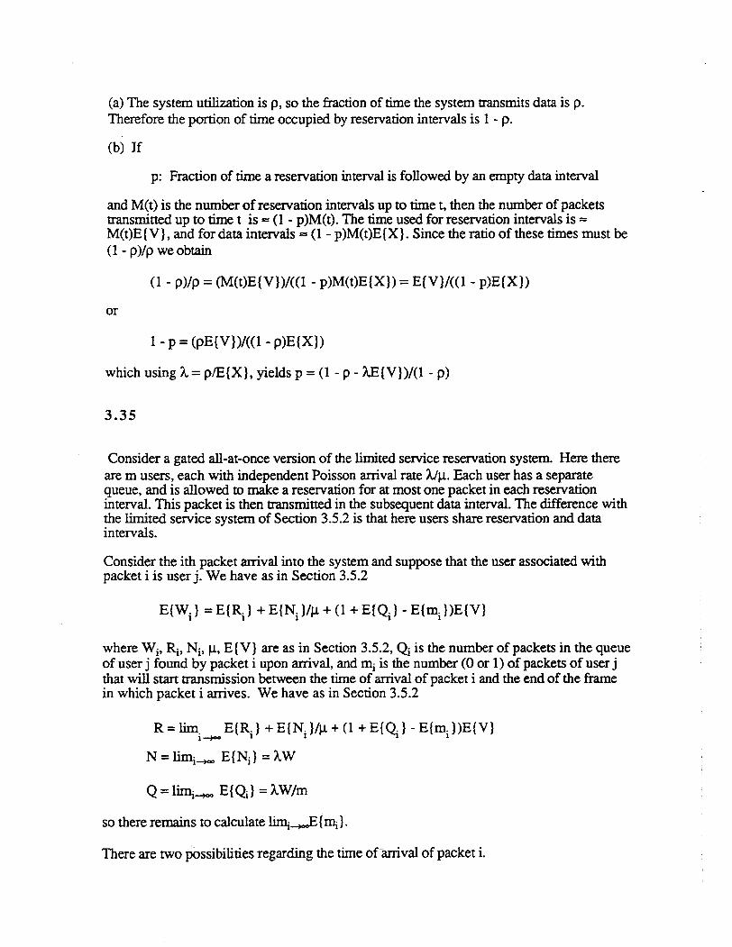
(a) The system utilization is p, so the fraction of time the system transmits data is p.Therefore the portion of time occupied by reservation intervals is 1 - p.

(b) If

p: Fraction of time a reservation interval is followed by an empty data interval

and M(t) is the number of reservation intervals up to time t, then the number of packetstransmitted up to time t is =(l - p)M(t). The time used for reservation intervals is =M(t)E{V}, and for data intervals == (1- p)M(t)E{X}. Since the ratio of these times must be(l - p)fp we obtain

(l - p)fp =(M(t)E{V})f«(1 - p)M(t)E{X}) =E{V}/«l - p)E{X})

or

1 - P = (pE{V})f«1 - p)E{X})

which using A= plE{X}, yields p = (1 - P - A.E{V})f(1 - p)

3.35

Consider a gated all-at-once version of the limited service reservation system. Here thereare m users, each with independent Poisson arrival rate A./J.l. Each user has a separatequeue, and is allowed to make a reservation for at most one packet in each reservationinterval. This packet is then transmitted in the subsequent data interval. The difference withthe limited service system of Section 3.5.2 is that here users share reservation and dataintervals.

Consider the ith packet arrival into the system and suppose that the user associated withpacket i is user j. We have as in Section 3.5.2

E{W.} =E{R.} +E{N.}/J.l+{l +E{Q.} -E{m.})E{V}1 1 1 1 1

where Wj, ~, Nj, J.l, E{V} are as in Section 3.5.2, Qj is the number of packets in the queueof user j found by packet i upon arrival, and mj is the number (0 or 1) of packets of user jthat will start transmission between the time of arrival of packet i and the end of the framein which packet i arrives. We have as in Section 3.5.2

R=lim. E{R.} +E{N.}/J.l+{l +E{Q.} -E{m.})E{V}1-+00 1 1 1 1

N =lim· E{N·} =AW1-+00 1

Q= limj-+oo E{Q} = AW/m

so there remains to calculate~~{mj}.

There are two possibilities regarding the time ofarrival of packet i.

a) Packet i arrives dming a reservation interVal. This event, call it A, has steadystate probability (l-p)

PtA} = I-p.

Since the ratio of average data interVa11ength to average reservation interVa1lengthis p/(l-p) we see that the average steady state length ofa data interVal is pE{V)/(l­p). Therefore the average steady state number ofpackets per user in a data interValis pE{V}/«I-p)mE{X}) =AE{V}/((l-p)m). This also equals the steady state valueofE{mJ A) in view of the system symmeny with respect to users

lim. E{m.! A) = AElV) .l-too 1 (1 - P)m

b) Packet i arrives dming a data interval. This event, call it B, has steady stateprobability p

PCB) =p.

Denote

a = ~-too E(lDj I B),

~= liIDj-too E(lDj I B, the data interval of arrival ofpacket i contains kpackets}.

Assuming k > 0 packets are contained in the data interval ofanival, there is equalprobability 11k of arrival during the transmission of any one of these packets.Therefore

k

~ =~ ! k - n =k(k - 1) =k - 1 .~k m 2km mn=1

Let P(k) be the unconditional steady-state probability that a nonempty data intervalcontains k packets, and E(k)and E(k2 ) be the corresponding fU'St two moments.Then we have using Bayes' rule

~-too P(The data interval of arrival of packet i contains k packets) = kP(k)IE(k).

Combining the preceding equations we have

_~ kP(k) _~ P(k)k(k - 1) _ E{k2} _..!..

a - £.J E{k} ak - ~ 2E{k}m - 2mE{k} 2m'k=l Ie=l

We have already shown as part of the analysis of case a) above that

E{k} =A.E{V}/(l - p)

so there remains to estimate E{k2}. We have

m

E{k2

} =L k2P(k)

k=l

H we maximize the quantity above over the distribution P(k), k =0,1,..., m subjectto the constraints r.~l kP(k) =E{k}, r.~=o P{k) =1, P{k) ~ 0 (a simple linear .programming problem) we find that the maximum is obtained for P(m) =E{k}/m,P(O) =1 -E{k}/m, and P(k) = 0, k = 1,2,...,m-1. Therefore

E{k2} S mE{k}.

Similarly if we minimize E {k2} subject to the same constraints we find that theminimum is obtained for P(k'-l) =k' - Elk}, P{k) =1 - (k' - E{k}) and P(k') =0for k ¢ k' - 1, k' where k' is the integer for which k' - 1 S E{k} < k'. Therefore

E{k2} ~ (k' -1)2(k' - E{k}) + (k')2[l - (k' - E{k})]

After some calculation this relation can also be written

E{k2} ~ Elk} + {k' -1)(2E{k} - k') for. E{k} E (k' - 1, k'),k' =1, 2, ..., m

Note that the lower bound above is a piecewise linear function ofE{k}, and equals(E{k})2 at the breakpoints k' =1,2,...,m. Summarizing the bounds we have

E{k) + {k' - 1)(2E{k} - k') 1 1 12mE{k} - 2m S a S 2' - 2m '

where k' is the positive integer for which

k' - 1 S E{k} < k' .

Note that as E{k} approaches its maximum value m (i.e., the system is heavilyloaded), the upper and lower bounds coincide. By combining the results for casesa) and b) above we have

lim. E{m.) = peA} lim. Elm.! A} +P{B} lim. Elm IB}I~ 1 . I~ 1 I-+- 1

= (l-p) AB{V} +pa(1- p)In

or finally

lim E{ }AB{V}

m = +pai~ 1 m

where a satisfies the upper and lower bounds given earlier. By taking limit as i -+00 in the equation

E{Wj } = E{~} + E{Nd/JJ. + (l + E{Q) - E{Illj})E{V)

and using the expressions derived we finally obtain

where a satisfies

E{k} + (k' - 1)(2E{k) - k') _...!... < <.!. _...!...2mE{k} 2m _(1 - 22m'

E{k) is the average number of packets per data interval

E{k} = A.E{V)/(l- p)

and k' is the integer for which k' - 1 S E{k} < k'. Note that the formula for thewaiting time W becomes exact in the limit both as p -+ 0 (light load), and as p -+ 1- AE{V}/m (heavy load) in which case E{k} -+ m and a-+ 112 -112m. When m =1 the formula for W is also exact and coincides with the one derived for thecorresponding single user one-at-a-time limited service system.

3.36

For each session, the arrival rates, average transmission times and utilization factors for theshort packets (class 1), and the long packets (class 2) are

Al = 0.25 packets/sec,~ = 2.25 packets/sec,

1/~1 =0.02 sees,1/JJ.2 = 0.3 sees,

PI =0.005P2 =0.675.

The corresponding second moments of transmission time are

NQ2 ="-2*w2 =0.855Nz= "-2*Tz = 2.273.

The total arrival rate for each session is A= 2.5 packets/sec. The overall 1st and 2ndmoments of the transmission time, and overall utilization factors are given by

1/~ =0.1 *(1/~}) + 0.9*(l/~2) =0.272E{X2} = 0.1 *E{X}2} + 0.9*E{X22} = 0.081P =A/~ =2.5*0.272 =0.68.

We obtain the averagetime in queue W via the P - K formula W = (A.E{X2})/(2*(l- p» =0.3164. The average time in the system is T = 1/~ + W = 0.588. The average number inqueue and in the system are NQ =AW =0.791, and N =AT = 1.47.

The quantities above correspond to each session in the case where the sessions are time ­division multiplexed on the line. In the statistical multiplexing case W, T, NQand N aredecreased by a factor of 10 (for each session).

In the nonpreemptive priority case we obtain using the corresponding fonnulas:

W} =(AIE{XI2} + AzE{X22})/(2*(l - PI» =0.108

Wz =(AIE{XI2} + "-2E{X22})/(2*(l- PI)*(l - PI - pz» =0.38

T} = l/~} + WI =0.128Tz= 1/~z + Wz = 1.055NQI = Al*W1 = 0.027NI =AI*TI =0.032

3.37

(a)A= 1/60 per secondE(X) = 16.5 secondsE(X2) = 346.5 secondsT = E(X) + AE(X2)/2(l-AE(X»

= 16.5 + (346.5/60)/2(1- 16.5/60) = 20.48 seconds

(b) Non-Preemptive Priority

In the following calculation, subscript 1 will imply the quantities for the priority 1customers and 2 for priority 2 customers. Unsubscripted quantities will refer to the overallsystem.

E(X) = 16.5, E(XI

) = 4.5, E(X2 ) = 19.5

EW) = 346.5

1 2R = 2 AE(X ) = 2.8875

PI = \ E(XI ) = 0.015

P2=1..

2E(X2) =0.26R

WI =- = 2.931I-pR

I

W2 =-- = 4.043I-P

2

TI = 7.4315, T2 = 23.543AT +AT

T= 1 1 2 2 =20.217A

(c) Preemptive Queueing

The anival rates and service rates for the two priorities are the same for preemptivesystem as the non-preemptive system solved above.

2 2E(Xl) = 22.5, E(X2 ) = 427.5

1 2R1 =2 \ E(X1) =0.0075

1 2~ = R1+ 21..

2E(X2) = 2.8575

E(X1)(l-p ) + R}

T = 11

I-p1

E(X2)(l-P -p ) +~T = 1 2

2 (l-p )(l-p -p )1 1 2

3.38

(a) The same derivation as in Section 3.5.3 applies for Wk, Le.

where Pi = ~/(IllJl), and R is the mean residual service time. Think of the system as beingcomprised of a serving section and a waiting section. The residual service time is just thetime until any of the customers in the waiting section can enter the serving section. Thus,the residual service time of a customer is zero if the customer enters service immediatelybecause there is a free server at the time of arrival, and is otherwise equal to the timebetween the customer's arrival, and the first subsequent service completion. Using thememoryless property of the exponential distribution it is seen that

R = PoE{Residual service time Iqueueing occurs} = Pd(m~).

(b) The waiting time of classes 1, ..., k is not influenced by the presence of classes(k+1), ... ,n. All priority classes have the same service time distribution, thus,interchanging the order of service does not change the average waiting time. We have

W(k) = Average waiting time for the M/MIm system with rate A.l + ... + A.k·

By Little's theorem we have

Average number in queue of class k = Average number in queue of classes 1 to k- Average number in queue of classes 1 to k-l

and the desired result follows.

3.39

Let k be such that

PI + ... + Pk-l S; 1 < PI + ... + Pk'

Then the queue of packets of priority k will grow infmitely, the arrival rate of each priorityup to and including k-1 will be accomodated, the departure rate of priorities above k will bezero while the departure rate of priority k will be

- (l-p -"'-p )Ax= 1 k-lXk

In effect we have a priority system with k priorities and arrival rates

-A' = A· for i < k1 1

- (l-Pl-···-PI.:-l)AI.:= XI.:

For priorities i < k the arrival process is Poisson so the same calculation for the waitingtime as before gives

k

I~XtVV.= ~l

1 2(1 - PI - ... - PH)(1- PI - ... - pr i<k

For priority k and above we have infinite average waiting time in queue.

3.40

(a) The algebraic verification using Eq. (3.79) listed below

is straightforward. In particular by induction we show that

R(PI + + pIJP W + ... + P W - ------.-;;;..Ilk k - 1 - PI - ... - Pk

The induction step is carried out by verifying the identity

The alternate argument suggested in the hint is straightforward.

(b) Cost

VVe know thatWI ~ W2 ~ ..... ~ Wn. Now exchange the priority of two neighboringclasses i and j=i+1 and compare C with the new cost

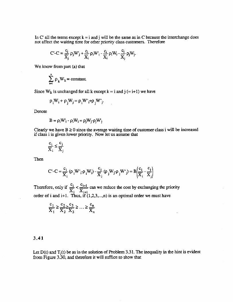
In C' all the terms except k = i and j will be the same as in C because the interchange doesnot affect the waiting time for other priority class customers. Therefore

C'-c = 5.. p·W'o +.s.. p·W'· - .s.. poW,o - 5... p,W·- J J - I I - I I - J J.Xj Xi Xi Xj

We know from pan (a) that

n

L PkWk = constantltzl

Since Wk is unchanged for all k except k = i andj (= i+l) we have

PiWi + pjWj = piW'j"+pjW'j.

Denote

B = PiWi - PiWi =PjWrPjWj

Clearly we have B ~ 0 since the average waiting time of customer class i will be increasedif class i is given lower priority. Now let us assume that

Then

c· c· (c. Co)C'-c = I (p .W'I'-P .WI·) - J (p .WJ._p oW'J) = B I _ JXo I I X' J J X· X.

I J I J

Therefore, only if ci < ci+l can we reduce the cost by exchanging the priorityXi X i+l

order of i and i+1. Thus, if (l,2,3,....n) is an optimal order we must have

..:.L> C2> c3 > > cnXl -X

2-X

3-"·-X

n

3.41

Let D(t) and Ti(t) be as in the solution of Problem 3.31. The inequality in the hint is evidentfrom Figure 3.30. and therefore it will suffice to show that

lim 2.~T.=lim 2.~T.t~ t.£..J 1 t~ t ~ 1

ieLXt) 1=1

We first show that

(1)

as k --+ 00 (2)

where tk is the arrival time of the kth customer. We have by assumption

and by taking the limit ask~ in the relation

(k+l)!tk+1 - kltk = 1/tk+1 - «tk+1 - tk)!tk+1)(kltk)

we obtain

as k --+ 00 (3)

We also have

sok +1 k

I, T. I,Tj1j=l i=l --+0lx+1 lx

or

k

~T.T ~ I t2.:!:!.. + 1=1 (__'1< _ 1) --+ 0~+1 lx \+1

which proves (2).

as k --+ 00 (4)

Let E > 0 be given. Then, from (2), there exists k such that T j < lj E for all i > k. Choose tlarge enough so that a(t) > k. Then

13(t) t a¢)

~~ S !r(t)dt s~~.. i=1 i=l

or

P(t) o.(t)

~ ~PCt) i=l S .!.ltr('t)d'ts a(t).!=!-..t pet) tot act)

Under the assumptions

we have

R=A.M

where

R = lim 1.rr(t)dtt....oo t.lo

is the time average rate at which the system earns. .

(b) Take ri(t) =1 for all t for which customer i resides in the system, and ri(t) = 0 for allother t.

(c) IfXi and Wi·are the seIVice and queueing times of the ith customer we have

where the two terms on the right above correspond to payment while in queue and seIVicerespectively. Applying pan (a) while taking expected values and taking the limit as i -+ 00,

and using the fact that Xi and Wi are independent we obtain

where U, the rate at which the system earns, is the average unfinished work in the system.Since the anival process is Poisson, U is also the average unfInished work seen by anarriving customer. Therefore U = W, and the p: K formula follows.

3.43

We have similar to Section 3.5

W=R+ pW+ WB

where the mean residual service time is

(1)

We derive the average waiting time of a customer for other customers that arrived in thesame batch

WB= LAE{WB Ibatchh~ sizej}j

where

Pj =Probability a batch has size jrj == Proportion of customers arriving in a batch of size j

We have

jP·=~

n

Also since the customer is equally likely to be in any position within the batch

Thus from (2)

Substituting in (1) we obtain

-R WBW=--+-­

1-p 1-p

- 2 - 2" -AnX x(n - n)

= 2(1 ) +- p 2n(l - p)

3.44

(a) Let Po be the steady state probability that an arriving packet finds the system empty.Then, in effect, a packet has service time X with probability 1 - Po, and service time X + /1with probability Po. The fraction of time the system is busy is obtained by applying Little'sTheorem to the service portion of the system

A[E{X}(l - Po) + (E{X} + E{/1})Pol = A(E{X} + E{/1}po)

This is also equal to P{system busy} == 1 - Po, so by solving for Po' we obtain

Po =(l - AE{X})/(l + AE{/1}) =(l - p)/(l + A.E{/1})

where p = A.E{X}.

(b) Let

E {I} =average length of an idle periodE{B} = average length of a busy period

Since the arrival process is Poisson we have

E{I} =l/A. =average time betwen last departure in a busy period and thenext arrival in the system

E{I} 1(A. 1 - AE{X}Po = E{I} + E{B} = 1/A+ E{B} = 1 + AE{~}

E{B} = E{X} + E{~} =E{X} + E{~}

1 - E{X}A 1 - P

(c) We calculate the mean residual time using a graphical argument

From the figure we have

where ~(i) is the service time of the first packet of the ith busy period, and

M(t) =# ofarrivals up to tN(t) = 4# of busy periods up to t

Taking the limit as t-+oo, and using the fact

Iim N(t)_l-Po_ A(l-p)t....oo t - E{B} - 1+ AE{6}

we obtain

We have, as in Section 3.5, W = R +pW or

W=RJ(l- p)

Substituting the expression for R obtained previously we obtain

't

AE{X2} A 2 2

W = 2(1- p) + 2(1 + AE{~}) [E{(X +~) } - E{X }]

3.45

(a) It is easy to see that

Pr (system busy serving customers) =p

Pr (system idle) = I-p = P(O in system) + P(l in idle system) + ...+ P(k:-l in idle system)

It can be seen that

P(O in system) = pel in idle system) =... = P(k-l in idle system) =(l-p)/k

implying that(l-p )(k-l)

P(nonempty and waiting) = k

(b) A busy period in this problem is the length of time the system is nonempty" The end of

each busy period is a renewal point for the system. Between two renewal points, the

system is either waiting (with 0 or more customers) or serving.

Let W be the expected length of a waiting period.Since arrivals are poisson, we have

- kW =-

J..,"

Let S be the expected length of a serving period.

Then the probability that the system is serving =p = SS+W

implying that

l-l = WP S

or_ pk

S=pW=~l-p I-p

Let j be the expected length of time the system is empty.

The expected length of a busy period = S + W - j

= p(kJA.) + k _1l-p A A

_pk+(l-p)(k-l)_ k+p-I- A(1-p ) - A(1-p )

PI~) is k times the average length of an MlG/1 busy period and k~I

is the average time from the first arrival until the system starts serving.

(c) We will call the k packets that are in the system at the beginning of the busy period"old" packets. Those that come during the busy period (and are therefore served duringthis period) are called "new" packets.

We consider the following service discipline: the server transmits old packets only when itdoesn't have new packets available at that moment (so it's not FCFS). Since this disciplinedoesn't depend on the length of the packets it will give the same average number of packetsin the system. Thus a busy period looks as illustrated below:

b1 b2 bk-1 bk.- - .- - - .- - - -- ... - p

- - - ... - - - - - - - - ....- _I.-~- ... 1- P

P P

old 1 new old 2 new old3 old k-1 new old k new

- -po

Busy period

In a subperiod bi of the busy period, the old packet i and the new packets combine to givethe same distribution as a normal MlG/1 busy period except that there are an extra k-i oldpackets in the system. It is easy to see that the distribution of the length of bi,b2, ... bk isthe same since each of them is exactly like an MlG/1 busy period.

~ E(N I serving) = E(N I bI) P(b} I serving) + ... + E(N I b0 P(bk I serving)

P(bi I serving) = ~

E(N I bi) = E(NM/G/l I busy) + k-iimplying that

E(N I serving) =~ (k E(NM/G/l I busy) + .f (k-i»)l 1=1

k-l=""2+ E(NMIG/l 1busy)

We have

E(NM/G/l) =E(NM/G/l I busy) P

from which

E(NM/G/ll busy) =E(NMlGll)P

or

E(N I .) E(NM/<m) k-lservmg = +T

P

Also

E(N I busy waiting) =E(N I waiting with 1) P(waiting with 11 busy waiting) + ...

+ E(N Iwaiting with k-I) P(waiting with k-II busy waiting)

P(waiting with i J busy waiting)

=P(waiting withj I busy waiting) =k~l for all 0 < i,j < k

from which

1 k-l kE(N Ibusy waiting) =k-l .L i =2

1=1

(d) E(N) =E(N J busy waiting) P(busy waiting) + E(N I busy serving) P(busy serving)

_!. (k-I) (I-p) (E.(NM/Gll) k-l)-2 k + ~ P + 2 P

k-l= E(NM/G/l) +T

3.46

We have

W=RI(l- p)

where

{

M(t) 1.(t) V2}R = lim ~,,~XZ+ ~"~

t-+oo t £..J2 1 t £..J 2i=l i=l

where L(t) is the number of vacations (or busy periods) up to time t. The average length ofan idle period is

and it can be seen that the steady-state time average number of vacations per unit time

We have

Therefore

and

3.47

1.(t) 2~v.

1.(t) 2 £-J 2:1,"" 1.~ Vi =lim L(t) ..:...i==--l_~"'t~t t 2 t~ t L(t)

_ A'Xl + V2(l -p)R- 2 21

w= A'Xl + Vl2(1 - p) 21

lin\ L(t) yz = V2(l -p)~t 21 21

(a) Since arrival times and service times are independent, the probability that there was anarrival in a small interval 0 at time 't - x and that this arrival is still being served at time 't isAo[l - Fx(x)).

(b) Wehave

-X =JxdFx(x)

o

and by calculating the shaded area of the figme below in two different ways we obtain

- -fxdFx(x) =J[1 - Fx(x)]dxo 0

This proves the desired expression.

x x+dx x

(c) Let Pn(x) be the steady state probability that the number of anivals that occUlTed prior totime 't - x and are still present at time 't is exactly n.

.For n ~ 1 we have

Pn(x - 0) = (1 - A[l- Fx(x)]O}Pn(x) + A[1 - Fx (x)]OPn_l(X)

and for n =0 we have

po(x - 0) = (1 - A[l - Fx(x)]O}po(x).

Thus Pn(x), n =0, 1, 2, ... are the solution of the differential equations

dpJdx = a(x)pn(x) - a(x)Pn_l(x) for n ~ 1

dP<ldx = a(x)po(x)

where

a(x) =1..[1 - Fx(x)].

Using the known conditions

for n =0

Pn(OO) = 0Po(oo) =1

forn ~ 1

it can be verified by induction starting with n =0 that the solution is

Since

--ja(y)dy [J a(y)dyt

Pn(x) = [e II ] x n! x ~ 0, n =0, I, 2, ...

- -f a(y)dy = A.J [l - Fx(x)]dy = A.E{X}o 0

we obtain

Pn(O) =e-AE(X) [A.E{~}t ,n.

n =0, 1,2, ...

Thus the number of anivals that are still in the system have a steady state Poissondistribution with mean AE{X}.

3.48

(a) Denote

f(x) =Er[(max{O,r-x})2]

and

g(x) =(Er[max{O,r-x}])2,

where ErH denotes expected value with respect to r (x is considered constant). We willprove that f(x)/g(x) is montonically nondecreasing for x nonnegative and thus attain itsminimum value for x=O. We have

a~~) = E~:X (maX{O,r-xn2] = 2E1maX{O,r-X)' :X (max{O,r-xn],

where

a(max{O,r-x}) =_u(r-x)ax

where u(') is the step function. Thus

af(x)ax=-2Er [(max(O,r-x})· u(r-x)] =-2EJmax{O,r-x}]

Assume for simplicity that r has a probability density function (the solution is similar in themore general case). Then

Thus

~~) g(x) - f(x)a!~) =2Er lmax{O,r-x}JEr [(max(O,r-x})2]Irxp(r)dr

- 2Er[max{O,r-x}]E,.([max{O,r-x}])2

For ~~~ monotonically nondecreasing we must have a~~) g(x) - f(x) a~~) ~ 0 or equivalently

Er [(maX{o,r-x})1J p(r)dr - (Er[max{O,r-x}]) 2r~

which is true by Schwanz's inequality. Thus the ratio

f(x) Er[(max{O,r-x})2]

g(x) = (Er[max{O,r-x}])2

is monotonically nondecreasing and attains its minimum value at x=O. On the other hand,we have

(1)

since r ~ 0, and the result follows.

(b) We know (cf. Eq. (3.93» that

Ik =-min{O,Wk + Xk - 'tk} =max{O,'tk - Wk - Xk}

=max{O,'tk- SkI,

where Sk is the time in the system. Since the relation in part (a) holds for any nonnegativescalar x, we can take expected values with respect to x as well, and use the fact that for anyfunction of x, g(x), E(g(x)2) ~ E2(g(x», and find that

Erx[(max{O,r-x})2] ~£.. <Erx[max{0,r-x}])2.• (r2) •

where x is considered to be a random variable this time. By letting r = 'tic. x = Sk. andk~oo,we find from (I) that

or

12 -(1)2 >~ - (t)2

(1)2 fi)2

or-2

~2 > (I) ~2'II - Va('t)2

(since a; is defined as the variance of intermival times)

Since j = l-p and t =.! we getA A

a~ ~ (l_p)2 a~

By using Eq. (3.97), we then obtain

< A(a; + a~ A(l-p) a;W - 2(1-p) - 2

A.E[X] = E[B]/(E[B]+If)...) ;

3.49

(a) Since the arrivals are Poisson with rate A. the mean time until the next arrival startingfrom any given time (such as the time when the system becomes empty) is If)... The timeaverage fraction of busy time is AE,[X]. This can be seen by Little's theorem applied to theservice facility (the time average number ofcustomers in the server is just the time average

nfraction of busy time), or it can be seen by letting V'i represent the time the server is

i=Ibusy with the first n customers, dividing by the arrival time of the nth customer, and goingto the limit.

Let E[B] be the mean duration of a busy period and E[I] = If).. be the mean durationof an idle period. The time average fraction of busy time must be E[B]/(E[B]+E[I]). Thus

EOOE[B] = I - AE[X]

This is the same as for the FCFS M/G/1 system (Problem 3.30).

(b) If a second customer arrives while the first customer in a busy period is being served,that customer (and all subsequent customers that arrive while the second customer is in thesystem) are served before the first customer resumes service. The same thing happens forany subsequent customer that arrives while the first customer is actually in service. Thuswhen the fJISt customer leaves, the system is empty. One can view the queue here as astack, and the first customer is at the bottom of the stack. It follows that E[B] is theexpected system time given a customer arriving to an empty system.

The customers already in the system when a given customer arrives receive noservice until the given customer departs. Thus the system time of the given customerdepends only on its own service time and the new customers that arrive while the givencustomer is in the system. Because of the memoryless property of the Poisson arrivals andthe independence of service times, the system time of the given customer is independent ofthe number of customers (and their remaining service times) in the system when the givencustomer arrives. Since the expected system time of a given customer is independent of thenumber of customers it sees upon arrival in the system, the expected time is equal to theexpected system time when the given customer sees an empty system; this is E[B] asshown above.

(c) Given that a customer requires 2 units of service time, look first at the expected systemtime until I unit of service is completed. This is the same as the expected system time of acustomer requiring one unit of service (i.e., it is one unit of time plus the service time of allcustomers who arrive during that unit and during the service of other such customers).When one unit of service is completed for the given customer, the given customer is inservice with one unit of service still required, which is the same as if a new customerarrived requiring one unit of service. Thus the given customer requiring 2 units of servicehas an expected system time of2C. Extending the argument to a customer requiring n unitsof service, the expected system time is nCo Doing the argument backwards for a customerrequiring lin of service, the expected system time is C/n. We thus conclude that E[systemtime I X=x] = ex.(d) We have

3.50

00

E[B] =JCx dF(x) = CE[X];1

C= 1 _ AE[X]

(a) Since (Pj} is the stationary distribution, we have for all je S

P.i(~qji +~ CJji ) =~Pi<Iij +~ PJ~jiES ilS iES ilS

Using the given relation, we obtain for all jeS

p·Lq,,=LP·q··J lEi Jl lEi 1 .IJ

Dividing by L p. , it follows that_ 1lES

for all jeS, showing that {Pi} is the stationary distribution of the truncated chain.

(b) If the original chain is time reversible, we have PAii =PiQij for an i and j, so the

condition of part (a) holds. Therefore, we have PAii = PiQij for all states i andj of thetruncated chain.

(c) The fmite capacity system is a truncation of the two independent MIMIl queues system,which is time reversible. Therefore, by part (b), the truncated chain is also time reversible.The formula for the steady state probabilities is a special case of Eq. (3.39) of Section 3.4.

3.51

(a) Since the detailed balance equations hold, we have

Thus for i, j e Sk, we have

p. p.U

J q"=-Ul q.. <=> x.:O .. =x1jCl..k JI k IJ PJI I)

and it follows that the Xi. i e Sk satisfy the detailed balance equations. Also

Therefore, {Xi lie Sk} as defmed above, is the stationary distribution of the Markov chainwith state space St.

(b) Obviously

K K

LUk=LLPj=l.k=l k=l JESt

Also we have

UIRkm= 2, xJ-qjiUPJEStiES.

which in view of the fact XjUt =Pj for je St, implies that

UIRkm= ~ PR...'" J JI

JEStiES.

and

uJimk =~ XJjQ .•Um =~ q ..p.=~ q.. p.~ JI ~ JJ j ~ Jj jjES. jES. iES.iESt iESt JESt

(3)

Since the detailed balance equations Pj<iji =qijPi hold, we have

"" PR. .. = "" q..D.~ j jJ ~ Jl' I

JESt iES.iES. JESt

Equations (2)-(4) give

(1)

(2)

(4)

(5)

Equations (1) and (5) imply that {Uk I k=I,...,K} is the stationary distribution of theMarkov chain with states l,u.,k, and transition rates Cikm.

(c) We will deal only with Example 3.13. (Example 3.12 is a special case with k=m).

51

50-....;....---Io*-....-.....:._----:~____:"""""'-----..w::.L-~........._----.:.;.;...;;....-~ __----:.:.:.....,

For i =O,I,...,k we define Si as the set of states (i,O), (i,I),..., (i,m-i), (see Figure 1).Then the truncated chain with state space Si is

~ ~ ~1

SI0'~0'~ ~~8Al A} A}

We denote by rep) the stationary probability of state j of the truncated chain Si and we let

Then

Thus

or

Therefore.

X~i) = I-Pl.J '=0 12k . 0 1 2 .tJl 1.. ...... J=.. .....m-lJ I_pf*l

The transition probabilities of the aggregate chain are

.-1-1,., ~ (1) ~ (ll.- 'l 0)ql, 1+1 = ~ XJ. q .. =~ XJ, ' J\.2 = A2(l-Xm _~

Jl joej E S)iE S)tl

= AJ1- I-Pl pm-l)-=).,2 l--r/f -1\ I-p~·I+1 1 I-p~-l+l

The aggregate chain is given by the following figure.

Thus we have

1 molUl+l = P2. -PI Ul

I-p~·l+l

from which

1 1-1 ( 1" rn-j ) 1" m - 1 +1U - zn 1 - 1 U

1 - P2 j=O 1 rn-j+l - Pz 1 m+l 0

"1 "1Furthermore, we have

or

from which

1-p~+1

Uo = -~-l-n.r-+lk+l 1 ~

1-P2 _pm+1 . PI1-pz 1 1- Pz

PI

and

1 pm - l + lUI = UO p~ _-..:..-0..

1 --1-p~+ I

Thus

from which we obtain the product form

(d) We are given that the detailed balance equations hold for the truncated chains. Thus fori, je Sk, we have Piqij = Pjqji. Furthermore,

Thus {7tj Ije Sk} is the distribution for the truncated chain Sk and the result ofpan (a)holds.

To prove the result ofpan (b), we have to prove that the global balance equationshold for the aggregate chain, i.e.,

k k

LiikmUk= L UuRmk'~l ~l

or equivalently

k k

L L 7tjUkqji= L L Qij7tiUm

~ljES ...iES. m=l jESlriES.

For j E Sk, we have 1tjUk =Pj, and for i e Sm, we have1tiUm =Pi. so we must show

k k

L L Pjqji= L L qifi~ljES..iES. m=l jES.. iES.

or

(6)

Since {Pi} is the distribution of the original chain, the global balance equations

~ p.q.. =~ p.q..£.J J JI ~ I IJall i all i

By summing over all je Sk, we see that Eq. (6) holds. Since

and we just proved that the Uk'S satisfy the global balance equations for the aggregatechain, {Uk I k =1,...,K} is the distribution of the aggregate chain. This proves the resultof pan (b).

3.52

Consider a customer arriving at time tl and departing at time t2. In reversed system tenns,the arrival process is independent Poisson, so the arrival process to the left of t2 isindependent of the times spent in the system ofcustomers that arrived at or to the right oft2. In particular, t2 - tl is independent of the (reversed system) arrival process to the left oft2. In forward system terms, this means that t2 - tl is independent of the departure processto the left of t2.

3.53

(a) Ifcustomers are served in the order they arrive then given that a customer departs attime t from queue 1, the arrival time of that customer at queue 1 (and therefore the timespent at queue I), is independent of the departure process from queue 1 prior to 1. Sincethe depanures from queue 1 are arrivals at queue 2, we conclude that the time spent by acustomer at queue 1 is independent of the anival times at queue 2 prior to the customer'sarrival at queue2. These arrival times, together with the corresponding independent (byKleinrock's approximation) service times determine the time the customer spends at queue2 and the departure process from queue 2 before the customer's departure from queue 2.

(b) Suppose packets with mean service time 1/J! arrive at the tandem queues with some rateAwhich is very small (A. «J!). Then, the apriori probability that a packet will wait inqueue 2 is very small.

Assume now that we know that the waiting time of a packet in queue 1 wasnonzero. This information changes the aposteriori probability that the packet will wait inqueue 2 to at least 1/2 (because its service time in queue 1 will be less than the service timeat queue 2 of the packet in front of it with probability 1/l). Thus the knowledge that thewaiting time in queue 1 is nonzero, provides a lot of information about the waiting time inqueue 2.

3.54

It can be verified by checking the detailed balance equations that the MlM/l/m queue isreversible. Hence the arrival and departure process are the same. The arrival process isPoisson but with probability Pm an anival does not enter the system. Also since an externalarrival process is independent of the state of the system, the arrival process to the sytem isstill Poisson but with rate A(l - Pm). By reversibility we conclude that the depanureprocess is also Poisson with rate A(1 - Pm).

3.SS

Let

p = Al1 J!1

P =A.22 Jl2

=-A. + CPU P1- m servers -

~~ +JJ,

- I

VOJl2AP2

~=­P1

Using Jackson's Theorem and Eqs. (3.34)-(3.35) we fmd that

where

[

. ]_1m-l (mp l)n (mp l)m

Po= L n! + m!(l-p )n=O 1 .

3.56

(a) We have

P(Xn=i) = (l-p)pi; ~ p = AlJl

P(Xn=i, Dn=i) =P(Dn=j 1Xn=i) P(Xn=i) = J.!A(l_p)pi; ~l, j=l= 0; i=Oj=l= (l-J.!A)(I-p)pi; ~I,j=O

= I-p; i=O, j=O

(b) P(Dn=l) = Li=l fU\«l-p)pi = ~p = U

(e) P(X -·1 n_-I) P(Xn=i,Dn=1} =. n-1 .~- - P(Dn=I) (J.!A(1_p)pi 11M = (l_p)pi-l ; ~l

= 0; i=O

(d) P(Xn+I=i1 Dn=l) = P(Xn=i+ll Dn=l) = (l_p)pi ; ~O

In the [1I'st equality above, we use the fact that, given a departure between nA and (n+1).1,the state at (n+1).1 is one less than the state at nA; in the second equality, we use part d).Since P(Xn+I=i) = (l_p)pi, we see that Xn+l is statistically independent of the event Dn=1.It is thus also independent of the complementary event Dn=O, and thus is independent ofthe random variable On.

(e) P(Xn+l=i, Dn+l=i I Dn) = P(Dn+l=i I Xn+l=i, Dn}P(Xn+l=i I Dn}= P(Dn+l=j I Xn+I=i)P(Xn+l=i }

The first part of the above equality follows because Xn+1is the state of the Markov processat time (n+1).1, so that, conditional on that state, Dn+1 is independent ofeverything in thepast The second part of the equality follows from the independence established in e).This establishes that Xn+1, Dn+1 are independent ofDn; thus their joint distribution is givenby b).

(f) We assume the inductive result for k-l and prove it for k; note that part f establishes theresult for k=1. Using the hint,

P(Xn+Ic=il Dn+k-l=l, Dn+k-2,..., Dn}=P(Xn+k-l=i+ll Dn+k-I=I,Dn+k-2,·~·,Dn)P(Xn+k-l=i+l, Dn+k-l=1IDn+k-2,..., Dn}

=P(Dn+k-l=ll Dn+k-2,..., Dn}

P(Xn+k-l=i+ I,Dn+k-l=l)= P(Dn+k-l-l)

= P(Xn+k-1=i+1IDn+k-l=l) = P(Xn+k=i I Dn+t-l=l}

The third equality above used the inductive hypothesis for the independence of the pair(Xn+k-I.On+k-l) from Dn+k-2,...Dn in the numerator and the corresponding independenceof Dn+k-l in the denominator. From part e}, with n+k-l replacing n, P(Xn+t=i I Dn+k-l) =P(Xn+k=i), so

P(Xn+k=i1 Dn+k-I=I, Dn+k-2,..., Dn) = P(Xn+0

Using the argument in e}, this shows that conditional on Dn+k-2,..., Dn, the variable Xn+kis independent of the event Dn+k-l=1 and thus also independent of Dn+k-l=0. Thus Xn+kis independent of Dn+k-l,..., Dn. Finally,

P(Xn+t=i, Dn+k=i I Dn+k-l,"', Dn) = P(Dn+k=j IXn+k=i)P(Xn+k=i1 Dn+k- lo..., On)

= P(Dn+k=j I Xn+t=i}P(Xn+k=i)

which shows the desired independence for k.

(g) This shows that the departure process is Bernoulli and that the state is independent ofpast depanures; i.e., we have proved the flI'St tW.D parts of Burke's theorem without using

reversibility. What is curious here is that the state independence is critical in establishingthe Bernoulli property.

3.57

The session numbers and their rates are shown below:

Session Session number p Session rate xp

ACE 1 100/60= 5/3ADE 2 200/60 = 10/3BCEF 3 500/60 = 25/3BDEF 4 600/60 = 30/3

The link numbers and the total link rates calculated as the sum of the rates of the sessionscrossing the links are shown below:

Link

ACCEADBDDEBCEF

Total link rate

Xl = 5/3Xl + x3 = 30/3x2 = 10/3x4= 10x2+ x4 = 40/3x3 =25/3X3 + X4 = 55/3

For each link (ij) the service rate is

Jlij = 50000/1000 = 50 packets/sec,

and the propagation delay is Dij =2 x 10-3 sees. The total arrival rate to the system is

y = ~ Xi = 5/3 + 10/3 + 25/3 + 30/3 = 70/3

The average number on each link (i, j) (based on the Kleinrock approximation fonnula) is:

- ~jNi; - A. + "-iJ"~J", J-lij - ij

From this we obtain:

Link

ACCEADBD

Average Number of Packets on the Link

(5/3)/(150/3 - 5/3) + (5/3)(2/1000) = 5/145 + 1/3001/4 + 1/501/14 + 1/1501/4 + 1/50

DEBeEF

4/11 + 2/751/5 + 1/6011/19 + 11/300

The average total number in the system is N == 1:(ij) Nij == 1.84 packet The average delayover all sessions is T = Nfy = 1.84 x (3nO) = 0.0789 sees. The average delay of thepackets of an individual session are obtained from the fonnula

L [ A,.. 1 ]IJT = +-+0·P Jli.(JJ... - t.) J..l... IJ

(iJ) on p J IJ IJ IJ

For the given sessions we obtain applying this formula

3.S8

Session p

1234

Average Delay Tp

0.0500.0530.0870.090

We convert the systeminto a closed network with M customers as indicated in the hintThe (k+l)st queue corresponds to the "outside world". It is easy to see that the queues ofthe open systems are equivalent to the first k queues of the closed system. For example.when there is at least one customer in the (k+1)st queue (equivalently. there are less than Mcustomers in the open system) the anival rate at queue i is

kr·

~r _l_=r..~ m k I_1

. Furthermore. when the (k+1)st queue is empty no external arrivals can occur at any queuei, i = I.Z....,k. If we denote with p(nh....nIJ the steady state distribution for the opensystem. we get

J 1C)M-LnPfp~···~ ~k+l

G(M)otherwise

where

ri· 12kPi =J.L,l= , ,... , ,

and G(M) is the normalizing factor.

3.59

H we insert a very fast MIMII queue {JJ.-+oo) between a pair of queues, then the probabilitydistribution for the packets in the rest of the queues is not affected. H we condition on asingle customer being in the fast queue, since this customer will remain in this queue for1/J.L (~) time on the average, it is equivalent to conditioning on a customer moving fromone queue to the other in the original system.

H P(nlt...,nIJ is the stationary distti.bution of the original system ofk queues andP'(nl....,nk,nk+l) is the corresponding probability distribution after the insertion of the fastqueue k+l, then

.'." ...

P(n},...,nk I arrival) = P'(nl,...,nk, nk+l = 1 I nk+l = 1),

which by independence of nl, ...,nk, nk+l, is equal to P(nl,...,nk).

3.60

Let Vj =utility function ofjth queue.

We have to prove that

But from problem 3.65 we have

Thus it is enough to prove that

where Pj =max{pJ,..., Pk}. We have

= A(M)+B(M)

Since Pj = max{PI,u.,Pk} we have that

lim A(M) = 0M-+ooB(M) .

Thus, Eq. (1) implies that

or, denoting n'j = nj - 1,

(1)

limM

-+oo-..._+--+1Ij+,;...·__+Ilr'M-_-_1 _

G(M)

or

lim Pj G(M-1) = 1M-+oo G(M)

3.61

m

We have LP i = 1 .;.0

1

The arrival rate at the CPU is A!po and the arrival rate at the ith I/O pon is Ap/PO- ByJackson's Theorem, we have

m

II DiP(no. nt .....nm) = Pi (l - Pi)

i=o

wherep = A.Jlo PO

A n;and Pi=~

JliPOfori> 0

The equivalent tandem system is as follows:

, ~ l-------l' 1/0 1 ~

The arrival rate is A.. The service rate for queue 0 is IloPo and for queue i (i > 0) is JliP<lPi'

3.62

Let A.o be the arrival rate at the CPU and let Ai be the arrival rate at YO unit i. We have

Ai = PiI..O. i =I.....m.

Let

and

A"p.=_l. i=O.I •...•m.1 Jl j

By Jackson's Theorem. the occupancy distribution is

where G(M)is the nonnalization constant corresponding to M customers.

Let

AOU O=­J.lo

be the utilization factor of the CPU. We have

Uo=P(no~ 1)= It P(nO,nl, ... ,nm>11.....+..........

'D.a

= It'D·...,+_.....~1

P'D'.<l,p D, P D.o 1'" m

G(M)

G(M-l) 1 G(M-l)=Po G(M) =J.lo G(M)'

where we used the change of variables n'o =no-l. Thus the arrival rate at the CPU is

G(M-l)AO= G(M)

and the arrival rate at the I/O unit i is

p.G(M-l)Ai = I G(M)' i=I,... ,m.

3.63

(a) We have A= Nrr and

T=T1 +T2 +T3

where

T1 = Average time at first transmission lineT2 =Average time at second transmission lineT3 =z

We have

so

(1)

___N__ S; AS; __N__

N(X + Y) + Z x + y + Z .

Also

so finally

ASK,X

As 1y

N <'\ < . {K 1. __N__}_1\._nDn , ,

N(X+Y)+Z X Y X+Y+Z

(b) The same line of argument applies except that in place of (l) we have

XST1 S(N-K+l)X

3.64

(a) The state is determined by the number of customers at node 1 (one could use node 2just as easily). When there are customers at node 1 (which is the case for states 1,2, and3), the departure rate from node 1 is J1l; each such departure causes the state to decrease asshown below. When there are customers in node 2 (which is the case for states 0, 1, and2), the departure rate from node 2 is J12; each such depanure causes the state to increase.

~ ~. ~

~~E ~~J1} J1} J11

(b) Letting Pi be the steady state probability of state i, we have Pi =Pi-l p, where p =J.L2IJ.Ll.Thus Pi = POpi. Solving for po,

PO = [1 + p + p2 + p3]-l, Pi = PO pi; i=I,2,3.

(c) Customers leave node 1 at rate J1l for all states other than state O. Thus the timeaverage rate r at which customers leave node 1 is J1l (I-PO), which is

(d) Since there are three customers in the system, each customer cycles at one third the rateat which departures occur from node 1. Thus a customer cycles at rate r/3.

(e) The Markov process is a birth-death process_and thus reversible. What appears as adeparture from node i in the forward process appears as an arrival to node i in the backward

process. If we order the customers 1, 2, and 3 in the order in which they depart a node,and note that this order never changes (because of the FCFS service at each node), then wesee that in the backward process, the customers keep their identity, but the order is reversedwith backward departures from node i in the order 3,2, 1,3,2, 1, ....

3.65

Since J.lj(m) =J.lj for all m, and the probability distribution for state n =(nl....,nlJ is

rill J1Ir.

Pen) = ~(M)'

where

J...p.=_J

J J.l.J

The utilization factor Uj (M) for queue j is

U j(M) = 2, Pen) = --,-Dro---:G:-::(M~)--D +_+D lliti, .

U.Dj'O

Denoting nj = nj-l, we get

~ n l n'l nk

£- PI ...p ....p k . Pj p.G(M-I)U (M) - D,+.•+D't..·+D..tol-l J _ -::..,J=....".,...._

j - G(M) - G(M) .

3.66

Let Cj indicate the class of the ith customer in queue.

We consider a state (q,c2,...,Cn) such that J.lq :¢: J.lcn'

,C 1 ,C 2 ,no Cn

CIt C 2 ,... Cn ,

·~Cl,C2'."~

If the steady-state distribution has a product form then the global balance equations for thisstate give

P(CI)'''P(Cn)(Jlcl + Al +... + A.c) =p(c})"·P(Cn-I)A.cn

+ (JlIP(l) + J.12P(2) + .. + flcP(c» P(CI)· ..··P(cn)

or

P(Cn)(JlCI + Al + ... + ~) = A.cn + (JlIp(l) + Jl2P(2) + ... + Jlcp(c»· p(cn)

Denote

M = JlIP(l) + Jl2P(2) + ... + Il<:p(c)

Then

p(Cn)(JlcI +A) = Acn + M'p(cn)

or

Acp(c ) = D

n Jl +A-MCl

This is a contradiction because even if ACI =0, p(cn) still depends on Jlcl ' The

contradiction gives that Jlci =Jl =constant for every class. Thus we can model this

system by a Markov chain only if JlI =Jl2 =... = flc.

(b) We will prove that the detailed balance equations hold. Based on the following figure

state z2

n

Jlr""'"

c n r '".-

(CI, C 2 ,no Cn_t) - (Cl,C 2 ,mCn)

A.cp

\.. ~ \.. ~

state Z1

the detailed balance equations are

or

ACPc"'Pc =J.1 P "'Pc'II 1 ...1 Cll CI II

which obviously holds.