Embed Size (px)
Citation preview

Chapter 4
Data Structures and BasicAlgorithms
VLSI chip design process can be viewed as transformation of data from HDLcode in logic design, to schematics in circuit design, to layout data in physi-cal design. In fact, VLSI design is a significant database management prob-lem. The layout information is captured in a symbolic database or a polygondatabase. In order to fabricate a VLSI chip, it needs to be represented as acollection of several layers of planar geometric elements or polygons. These ele-ments are usually limited to Manhattan features (vertical and horizontal edges)and are not allowed to overlap within the same layer. Each element must bespecified with great precision. This precision is necessary since this informationhas to be communicated to output devices such as plotters, video displays, andpattern-generating machines. Most importantly, the layout information mustbe specific enough so that it can be sent to the fab for fabrication. Symbolicdatabase captures net and transistor attributes. It allows a designer to rapidlynavigate throughout the database and make quick edits while working at ahigher level. The symbolic database is converted into a polygon database priorto tapeout. In the polygon database, the higher level relationship between theobjects is somewhat lost. This process is analogous to conversion of a higherlevel programming language (say FORTRAN) code to a lower level program-ming language (say Assembly) code. While it is easier to work at symboliclevel, it cannot be used by the fab directly. In some cases, at late stages of thechip design process, some edits have to be made in the polygon database. Themajor motivation for use of the symbolic database is technology independence.Since physical dimensions in the symbolic database are only relative, the de-sign can be implemented using any process. However, in practice, completetechnology independence has never be reached.
The layouts have historically been drawn by human layout designers toconform to the design rules and to perform the specified functions. A physicaldesign specialist typically converted a small circuit into layout consisting of aset of polygons. These manipulations were time consuming and error prone,

98 Chapter 4. Data Structures and Basic Algorithms
even for small layouts. Rapid advances in fabrication technology in recentyears have dramatically increased the size and complexity of VLSI circuits. Asa result, a single chip may include several million transistors. These techno-logical advances have made it impossible for layout designers to manipulatethe layout databases without sophisticated CAD tools. Several physical designCAD tools have been developed for this purpose, and this field is referred toas Physical Design Automation. Physical design CAD tools require highly spe-cialized algorithms and data structures to effectively manage and manipulatelayout information. These tools fall in three categories. The first type of toolshelp a human designer to manipulate a layout. For example, a layout editorallows designers to add transistors or nets to a layout. The second type of toolsare designed to perform some task on the layout automatically. Example ofsuch tools include channel routers and placement tools. It is also possible toinvoke a tool of second type from the layout editor. The third type of toolsare used for checking and verification. Example of such tools include; DRC(design rule checker) and LVS verifier (layout versus schematics verifier). Thebulk of the research of physical design automation has focused on tools of thelast two types. However, due to broad range and significant impact the tools ofsecond type have received the most attention. The major accomplishment inthat area has been decomposition of the physical design problem into severalsmaller (and conceptually easier) problems. Unfortunately, even these prob-lems are still computationally very hard. As a result, the major focus has beenon development on design and analysis of heuristic algorithms for partitioning,placement, routing and compaction. Many of these algorithms are based ongraph theory and computational geometry. As a result, it is important to havea basic understanding of these two fields. In addition, several special classesof graphs are used in physical design. It is important to understand propertiesand algorithms about these classes of graphs to develop effective algorithms inphysical design.
This chapter consists of three parts. First we discuss the basic algorithmsand mathematical methods used in VLSI physical design. These algorithmsform the basis for many of the algorithms presented later in this book. In thesecond part of this chapter, we shall study the data structures used in layouteditors and the algorithms used to manipulate these data structures. We alsodiscuss the formats used to represent VLSI layouts. In the third part of thischapter, we will focus on special classes of graphs, which play a fundamentalrole in development of these algorithms. Since most of the algorithms in VLSIphysical design are graph theoretic in nature, we devote a large portion ofthis chapter to graph algorithms. In the following, we will review basic graphtheoretic and computation geometry algorithms which play a significant rolein many different VLSI design algorithms. Before we discuss the algorithms,we shall review the basic terminology.

4.1. Basic Terminology 99
4.1 Basic Terminology
A graph is a pair of sets G = (V, E), where V is a set of vertices, and E isa set of pairs of distinct vertices called edges. We will use V(G) and E(G) torefer to the vertex and edge set of a graph G if it is not clear from the context.A vertex is adjacent to a vertex if is an edge, i.e., Theset of vertices adjacent to is An edge is incident on thevertices and which are the ends of The degree of a vertex is thenumber of edges incident with the vertex
A complete graph on vertices is a graph in which each vertex is adjacentto every other vertex. We use to denote such a graph. A graph is calledthe complement of graph G = (V, E) if H = (V, F), where,
A graph is a subgraph of a graph G if and only if andIf and then is a vertex induced
subgraph of G. Unless otherwise stated, by subgraph we mean vertex inducedsubgraph.
A walk P of a graph G is defined as a finite alternating sequenceof vertices and edges, beginning and ending with vertices, such
that each edge is incident with the vertices preceding and following it.A tour is a walk in which all edges are distinct. A walk is called an open
walk if the terminal vertices are distinct. A path is a open walk in which novertex appears more than once.
The length of a path is the number of edges in it. A path is a path ifand A cycle is a path of length where A cycle
is called odd if it's length is odd, otherwise it is an even cycle. Two verticesand in G are connected if G has a path. A graph is connected if all pairsof vertices are connected. A connected component of G is a maximal connectedsubgraph of G. An edge is called an cut edge in G if its removal from Gincreases the number of connected components of G by at least one. A tree isa connected graph with no cycles. A complete subgraph of a graph is called aclique.
A directed graph is a pair of sets where V is a set of vertices andis a set of ordered pairs of distinct vertices, called directed edges. We use thenotation for a directed graph, unless it is clear from the context. A directededge is incident on and and the vertices and are called thehead and tail of respectively. is an in-edge of and an out-edge ofThe in-degree of denoted by is equal to the number of in-edges ofsimilarly the out-degree of denoted by is equal to the number of out-edges of An orientation for a graph G = (V, E) is an assignment of directionfor each edge. An orientation is called transitive if, for each pair of edgesand there exists an edge If such a transitive orientation existsfor a graph G, then G is called a transitively orientable graph. Definitions ofsubgraph, path, walk are easily extended to directed graphs. A directed acyclicgraph is a directed graph with no directed cycles. A vertex is an ancestorof (and is a descendent of ) if there is a directed path in G. Arooted tree (or directed tree) is a directed acyclic graph in which all vertices

100 Chapter 4. Data Structures and Basic Algorithms
have in-degree 1 except the root, which has in-degree 0. The root of a rootedtree T is denoted by root(T). The subtree of tree T rooted at is the subtreeof T induced by the descendents of . A leaf is a vertex in a directed acyclicgraph with no descendents.
A hypergraph is a pair (V, E), where V is a set of vertices and E is a familyof sets of vertices. A hyperpath is a sequence ofdistinct vertices and distinct edges, such that vertices and are elementsof the edge Two vertices and are connected in a hypergraphif the hypergraph has a hyperpath. A hypergraph is connected if everypair of vertices are connected.
A bipartite graph is a graph G whose vertex set can be partitioned into twosubsets X and Y, so that each edge has one end in X and one end in Y; such apartition (X , Y) is called bipartition of the graph. A complete bipartite graph isa bipartite graph with bipartition (X , Y) in which each vertex of X is adjacentto each vertex of Y; if |X| = and |Y| = , such a graph is denoted byAn important characterization of bipartite graphs is in terms of odd cycles. Agraph is bipartite if and only if it does not contain an odd cycle.
A graph is called planar if it can be drawn in the plane without any twoedges crossing. Notice that there are many different ways of ‘drawing’ a planargraph. A drawing may be obtained by mapping a vertex to a point in theplane and mapping edges to paths in the plane. Each such drawing is calledan embedding of G. An embedding divides the plane into finite number ofregions. The edges which bound a region define a face. The unbounded regionis called the external or outside face. A face is called an odd face if it has oddnumber of edges. Similarly a face with even number of edges is called an evenface. The dual of a planar embedding T is a graph such the
v is a face in T} and two vertices share an edge if their correspondingfaces share an edge in T.
4.2 Complexity Issues and NP-hardness
Several general algorithms and mathematical techniques are frequently usedto develop algorithms for physical design. While the list of mathemat-ical and algorithmic techniques is quite extensive, we will only mention thebasic techniques. One should be very familiar with the following techniques toappreciate various algorithms in physical design.
1.
2.
3.
4.
5.
Greedy Algorithms
Divide and Conquer Algorithms
Dynamic Programming Algorithms
Network Flow Algorithms
Linear/Integer Programming Techniques

4.2. Complexity Issues and NP-hardness 101
Since these techniques and algorithms may be found in a good computerscience or graph algorithms text, we omit the discussion of these techniquesand refer the reader to an excellent text on this subject by Cormen, Leisersonand Rivest [CLR90].
The algorithmic techniques mentioned above have been applied to variousproblems in physical design with varying degrees of success. Due to the verylarge number of components that we must deal with in VLSI physical designautomation, all algorithms must have low time and space complexities. Foralgorithms which must operate on the entire layout even quadraticalgorithms may be intolerable. Another issue of great concern is the constantsin the time complexity of algorithms. In physical design, the key idea is todevelop practical algorithms, not just polynomial time complexity algorithms.As a result, many linear and quadratic algorithms are infeasible in physicaldesign due to large constants in their complexity.
The major cause of concern is absence of polynomial time algorithms formajority of the problems encountered in physical design automation. In fact,there is evidence that suggests that no polynomial time algorithm may exist formany of these problems. The class of solvable problems can be partitioned intotwo general classes, P and NP. The class P consists of all problems that can besolved by a deterministic turing machine in polynomial time. A conventionalcomputer may be viewed as such a machine. Minimum cost spanning tree,single source shortest path, and graph matching problems belong to class P.The other class called NP, consists of problems that can be solved in polyno-mial time by a nondeterministic turing machine. This type of turing machinemay be viewed as a parallel computer with as many processors as we mayneed. Essentially, whenever a decision has several different outcomes, severalnew processors are started up, each pursuing the solution for one of the out-comes. Obviously, such a model is not very realistic. If every problem in classNP can be reduced to a problem P, then problem P is in class NP-complete.Several thousand problems in computer science, graph theory, combinatorics,operations research, and computational geometry have been proven to be NP-complete. We will not discuss the concept of NP-completeness in detail, in-stead, we refer the reader to the excellent text by Garey and Johnson on thissubject [GJ79]. A problem may be stated in two different versions. For ex-ample, we may ask does there exist a subgraph H of a graph G, which has aspecific property and has size or bigger? Or we may simply ask for the largestsubgraph of G with a specific property. The former type is the decision versionwhile the latter type is called the optimization version of the problem. Theoptimization version of a problem P, is called NP-hard if the decision versionof the problem P is NP-complete.
4.2.1 Algorithms for NP-hard Problems
Most optimization problems in physical design are NP-hard. If a problemis known to be NP-complete or NP-hard, then it is unlikely that a polynomialtime algorithm exists for that problem. However, due to practical nature of the

102 Chapter 4. Data Structures and Basic Algorithms
physical design automation field, there is an urgent need to solve the problemeven if it cannot be solved optimally. In such cases, algorithm designers areleft with the following four choices.
4.2.1.1 Exponential Algorithms
If the size of the input is small, then algorithms with exponential time com-plexity may be feasible. In many cases, the solution of a certain problem becritical to the performance of the chip and therefore it is practical to spendextra resources to solve that problem optimally. One such exponential methodis integer programming, which has been very successfully used to solve manyphysical design problems. Algorithms for solving integer programs do not havepolynomial time complexity, however they work very efficiently on moderatesize problems, while worst case is still exponential. For large problems, algo-rithms with exponential time complexity may be used to solve small sub-cases,which are then combined using other algorithmic techniques to obtain the globalsolution.
4.2.1.2 Special Case Algorithms
It may be possible to simplify a general problem by applying some restrictionsto the problem. In many cases, the restricted problem may be solvable inpolynomial time. For example, the graph coloring problem is NP-complete forgeneral graphs, however it is solvable in polynomial time for many classes ofgraphs which are pertinent to physical design.
Layout problems are easier for simplified VLSI design styles such as stan-dard cell, which allow usage of special case algorithms. Conceptually, it ismuch easier to place cells of equal heights in rows, rather than placing arbi-trary sized rectangles in a plane. The clock routing problem, which is ratherhard for full-custom designs, can be solved in time for symmetric struc-tures such as gate arrays. Another example may be the Steiner tree problem(see Section 4.3.1.6). Although the general Steiner tree problem is NP-hard,a special case of the Steiner tree problem, called the single trunk steiner treeproblem (see exercise 4.7), can be solved in time.
4.2.1.3 Approximation Algorithms
When exponential algorithms are computationally infeasible due to the sizeof the input and special case algorithms are ruled out due to absence of anyrestriction that may be used, designers face a real challenge. If optimality is notnecessary and near-optimality is sufficient, then designers attempt to develop anapproximation algorithm. Often in physical design algorithms, near-optimalityis good enough. Approximation algorithms produce results with a guarantee.That is, while they may not produce an optimal result, they guarantee that theresult would never be worse than a lower bound determined by the performanceratio of the algorithm. The performance ratio of an algorithm is defined as
where is the solution produced by the algorithm and is the optimal

4.2. Complexity Issues and NP-hardness 103
solution for the problem. Recently, many algorithms have been developed withvery close to 1. We will use vertex cover as an example to explain the concept
of an approximation algorithm.Vertex cover is basically a problem of covering all edges by using as few
vertices as possible. In other words, given an undirected graph G = (V,E),select a subset such that for each edge either or orboth are in and has minimum size among all such sets. The vertex coverproblem is known to be NP-complete for general graphs. However, the simplealgorithm given in Figure 4.1 achieves near optimal results. The basic idea isto select an arbitrary edge and delete it and all edges incident on and
. Add and to the vertex cover set S. Repeat this process on the newgraph until all edges are deleted. The selected edges are kept in a set R.
Since no edge is checked more than once, it is easy to see that the algorithmAVC runs in O(| E |) time.
Theorem 1 Algorithm AVC produces a solution with a performance ratio of0.5.
Proof: Note that no two edges in R have a vertex in common, and |S| = 2 × |R|.However, since R is set of vertex disjoint edges, at least | R | vertices are neededto cover all the edges. Thus
In Section 4.5.6.2, we will present an approximation algorithm for findingmaximum k-partite subgraph in circle graphs. That algorithm is usedin topological routing, over-the-cell routing,via minimization and several otherphysical design problems.
4.2.1.4 Heuristic Algorithms
Faced with NP-complete problems, heuristic algorithms are frequently theanswer. A heuristic algorithm does produce a solution but does not guaran-

104 Chapter 4. Data Structures and Basic Algorithms
tee the optimality of the solution. Such algorithms must be tested on vari-ous benchmark examples to verify their effectiveness. The bulk of research inphysical design has concentrated on heuristic algorithms. An effective heuris-tic algorithm must have low time and space complexity and must produce anoptimal or near optimal solution in most realistic problem instances. Such algo-rithms must also have good average case complexities. Usually good heuristicalgorithms are based on optimal algorithms for special cases and are capable ofproducing optimal solutions in a significant number of cases. A good exampleof such algorithms are the channel routing algorithms (discussed in chapter 7),which can solve most channel routing problems using one or two tracks morethan the optimal solution. Although the channel routing problem in general isNP-complete, from a practical perspective, we can consider the channel routingproblem as solved.
In many cases, an time complexity heuristic algorithm has been devel-oped, even if an optimal or time complexity algorithm is knownfor the problem. One must keep in mind that optimal solutions may be hardto obtain and may be practically insignificant if a solution close to optimal canbe produced in a reasonable time. Thus the major focus in physical design hasbeen on the development of practical heuristic algorithms which can produceclose to optimal solutions on real world examples.
4.3 Basic Algorithms
Basic algorithms which are frequently used in physical design as subalgo-rithms can be categorized as: graph algorithms and computational geometrybased algorithms. In the following, we review some of the basic algorithms inboth of these categories.
4.3.1 Graph Algorithms
Many real-life problems, including VLSI physical design problems, can bemodeled using graphs. One significant advantage of using graphs to formulateproblems is that the graph problems are well-studied and well-understood.Problems related to graphs include graph search, shortest path, and minimumspanning tree, among others.
4.3.1.1 Graph Search Algorithms
Since many problems in physical design are modeled using graphs, it is im-portant to understand efficient methods for searching graphs. In the following,we briefly discuss the three main search techniques.
1. Depth-First Search: In this graph search strategy, graph is searched‘as deeply as possible’. In Depth-First Search (DFS), an edge is selectedfor further exploration from the most recently visited vertex . Whenall the edges of have been explored, the algorithm back tracks to the

4.3. Basic Algorithms 105
previous vertex, which may have an unexplored edge. Figure 4.4 is anoutline of a depth-first search algorithm. The algorithm uses an arrayMARKED ( ) which is initialized to zero before calling the algorithm tokeep track of all the visited vertices.
It is easy to see that the time complexity of depth-first search is O(| V | +|E|). Figure 4.2(c) shows an example of the depth first search for thegraph shown in Figure 4.2(a).
Breadth-First Search: The basic idea of Breadth-First Search (BFS)is to explore all vertices adjacent to a vertex before exploring any othervertex. Starting with a source vertex , the BFS first explores all edgesof , puts the reachable vertices in a queue, and marks the vertex asvisited. If a vertex is already marked visited then it is not enqueued. Thisprocess is repeated for each vertex in the queue. This process of visitingedges produces a BFS tree. The BFS algorithm can be used to searchboth directed and undirected graphs. Note that the main difference be-
2.

106 Chapter 4. Data Structures and Basic Algorithms
3.
tween the DFS and the BFS is that the DFS uses a stack (recursion isimplemented using stacks), while the BFS uses a queue as its data struc-ture. The time complexity of breadth first search is also O(|V| + |E|).Figure 4.2(b) shows an example of the BFS of the graph shown in Fig-ure 4.2(a).
Topological Search: In a directed acyclic graph, it is very naturalto visit the parents, before visiting the children. Thus, if we list thevertices in the topological order, if G contains a directed edge ,then appears before in the topological order. Topological search canbe done using depth first search and hence it has a time complexity ofO(| V| + |E |) . Figure 4.3 shows an example of the topological search.Figure 4.3(a) shows an entire graph. First vertex A will be visited sinceit has no parent. After visiting A , it is deleted (see Figure 4.3(b)) andwe get vertices B and C as two new vertices to visit. Thus, one possibletopological order would be A, B, C, D, E, F.
4.3.1.2 Spanning Tree Algorithms
Many graph problems are subset selection problems, that is, given a graphG = (V,E), select a subset such that has property Someproblems are defined in terms of selection of edges rather than vertices. Onefrequently solved graph problem is that of finding a set of edges which spansall the vertices. The Minimum Spanning Tree (MST) is an edge selectionproblem. More precisely, given an edge-weighted graph G = (V, E), selecta subset of edges such that induces a tree and the total cost ofedges is minimum over all such trees, where is the costor weight of the edge
There are basically three algorithms for finding a MST:
1.
2.
3.
Boruvka’s Algorithm
Kruskal’s Algorithm
Prim’s Algorithm.

4.3. Basic Algorithms 107
We will briefly explain Kruskal’s algorithm [Kru56], whereas the details of otheralgorithms can be found in [Tar83]. Kruskal’s algorithm starts by sorting theedges by nondecreasing weight. Each vertex is assigned to a set. Thus atthe start, for a graph with vertices, we have sets. Each set represents apartial spanning tree, and all the sets together form a spanning forest. Foreach edge from the sorted list, if and belong to the same set, theedge is discarded. On the other hand, if and belong to disjoint sets, anew set is created by union of these two sets. This edge is added to thespanning tree. In this way, algorithm constructs partial spanning trees andconnects them whenever an edge is added to the spanning tree. The runningtime of Kruskal’s algorithm in O(| E | log |E | ) . Figure 4.5 shows an example ofKruskal’s algorithm. First edge (D, F) is selected since it has the lowest weight(See Figure 4.5(b)). In the next step, there are two choices since there are twoedges with weight equal to 2. Since ties are broken arbitrarily, edge (D, E) isselected. The final tree is shown in Figure 4.5(f).
108 Chapter 4. Data Structures and Basic Algorithms
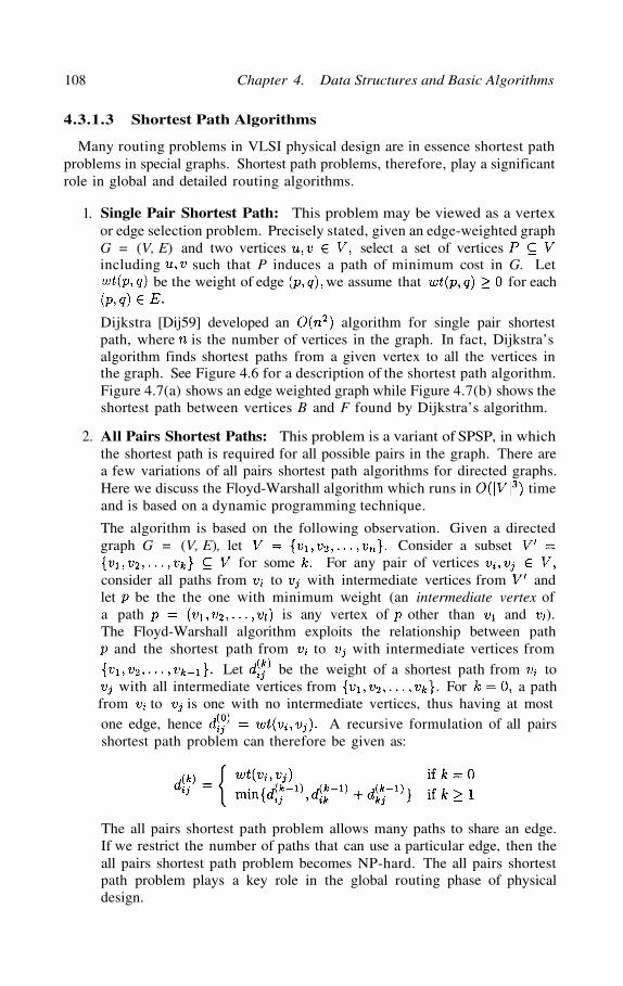
4.3.1.3 Shortest Path Algorithms
Many routing problems in VLSI physical design are in essence shortest pathproblems in special graphs. Shortest path problems, therefore, play a significantrole in global and detailed routing algorithms.
1.
2.
Single Pair Shortest Path: This problem may be viewed as a vertexor edge selection problem. Precisely stated, given an edge-weighted graphG = (V, E) and two vertices select a set of verticesincluding such that P induces a path of minimum cost in G. Let
be the weight of edge we assume that for each
Dijkstra [Dij59] developed an algorithm for single pair shortestpath, where is the number of vertices in the graph. In fact, Dijkstra’salgorithm finds shortest paths from a given vertex to all the vertices inthe graph. See Figure 4.6 for a description of the shortest path algorithm.Figure 4.7(a) shows an edge weighted graph while Figure 4.7(b) shows theshortest path between vertices B and F found by Dijkstra’s algorithm.
All Pairs Shortest Paths: This problem is a variant of SPSP, in whichthe shortest path is required for all possible pairs in the graph. There area few variations of all pairs shortest path algorithms for directed graphs.Here we discuss the Floyd-Warshall algorithm which runs in timeand is based on a dynamic programming technique.
The algorithm is based on the following observation. Given a directedgraph G = (V, E), let Consider a subset
for some . For any pair of verticesconsider all paths from to with intermediate vertices from andlet be the the one with minimum weight (an intermediate vertex ofa path is any vertex of other than and ).The Floyd-Warshall algorithm exploits the relationship between path and the shortest path from to with intermediate vertices from
Let be the weight of a shortest path from towith all intermediate vertices from For a path
from to is one with no intermediate vertices, thus having at mostone edge, hence A recursive formulation of all pairsshortest path problem can therefore be given as:
The all pairs shortest path problem allows many paths to share an edge.If we restrict the number of paths that can use a particular edge, then theall pairs shortest path problem becomes NP-hard. The all pairs shortestpath problem plays a key role in the global routing phase of physicaldesign.

4.3. Basic Algorithms 109

110 Chapter 4. Data Structures and Basic Algorithms
4.3.1.4 Matching Algorithms
Given an undirected graph G = (V, E), a matching is a subset of edgessuch that for all vertices at most one edge of is incident on
. A vertex is said to be matched by matching if some edge in is incidenton ; otherwise is unmatched. A maximum matching is a matching withmaximum cardinality among all matchings of a graph, i.e., if is a maximummatching in G, then for any other matching in Figure 4.8shows an example of matching. A matching is called a bipartite matching if theunderlying graph is a bipartite graph. Both matching and bipartite matchinghave many important applications in VLSI physical design. The details ofdifferent matching algorithms may be found in [PS82].
4.3.1.5 Min-Cut and Max-Cut Algorithms
Min-cut and Max-cut are two frequently used graph problems which arerelated to partitioning the vertex set of a graph.
The simplest Min-cut problem can be defined as follows: Given a graphG = (V, E), partition V into subsets and of equal sizes, such that thenumber of edges is minimized. The set is alsoreferred to as a cut. A more general min-cut problem may specify the sizes ofsubsets, or it may require partitioning V into different subsets. The min-cutproblem is NP-complete [GJ79]. Min-cut and many of its variants have severalapplications in physical design, including partitioning and placement.
The Max-cut problem can be defined as follows: Given a graph G = (V, E),find the maximum bipartite graph of G. Let be the maximumbipartite of G, which is obtained by deleting K edges of G, then G has amax-cut of size |E| – K.
Max-cut problem is NP-complete [GJ79]. Hadlock [Had75] presented analgorithm which finds max-cut of a planar graph. The algorithm is formallypresented in Figure 4.9. Procedure PLANAR-EMBED finds a planar embed-ding of G, and CONSTRUCT-DUAL creates a dual graph for the embedding.Procedure CONSTRUCT-WT-GRAPH constructs a complete weighted graphby using only vertices corresponding to odd faces. The weight on the edge
indicates the length of the shortest path between vertices and v in

4.3. Basic Algorithms 111
Note that the number of odd faces in any planar graph is even. ProcedureMIN-WT-MATCHING pairs up the vertices in R. Each edge in matching rep-resents a path in G. This path actually passes through even faces and connectstwo odd faces. All edges on the path are deleted. Notice that this operationcreates a large even face. This edge deletion procedure is repeated for eachmatched edge in M. In this way, all odd faces are removed. The resultinggraph is bipartite.
Consider the example graph shown in Figure 4.10(a). The dual of the graphis shown in Figure 4.10(b). The minimum weight matching of cost 4 is (3, 13)and (5, 10). The edges on the paths corresponding to the matched edges, in M,have been deleted and the resultant bipartite graph is shown in Figure 4.10(d).
4.3.1.6 Steiner Tree Algorithms
Minimum cost spanning trees and single pair shortest paths are two edgeselection problems which can be solved in polynomial time. Surprisingly, asimple variant of these two problems, called the Steiner minimum tree problem,is computationally hard.
The Steiner Minimum Tree (SMT) problem can be defined as follows: Givenan edge weighted graph G = (V, E) and a subset select a subsetsuch that and induces a tree of minimum cost over all such trees.
The set D is referred to as the set of demand points and the set isreferred to as Steiner points. In terms of VLSI routing the demand points arethe net terminals. It is easy to see that if D = V , then SMT is equivalent toMST, on the other hand, if |D| = 2 then SMT is equivalent to SPSP. UnlikeMST and SPSP, SMT and many of its variants are NP-complete [GJ77]. Inview of the NP-completeness of the problem, several heuristic algorithms have

112 Chapter 4. Data Structures and Basic Algorithms
been developed.Steiner trees arise in VLSI physical design in routing of multi-terminal nets.
Consider the problem of interconnecting two points in a plane using the shortestpath. This problem is similar to the routing problem of a two terminal net.If the net has more than two terminals then the problem is to interconnectall the terminals using minimum amount of wire, which corresponds to theminimization of the total cost of edges in the Steiner tree. The global anddetailed routing of multi-terminal nets is an important problem in the layoutof VLSI circuits. This problem has traditionally been viewed as a Steinertree problem [CSW89, HVW85]. Due to their important applications, Steinertrees have been a subject of intensive research [CSW89, GJ77, Han76, HVW85,HVW89, Hwa76b, Hwa79, LSL80, SW90]. Figure 4.11(b) shows a Steiner treeconnecting vertices A, I, F, E, and G of Figure 4.11 (a).
The underlying grid graph is the graph defined by the intersections of thehorizontal and vertical lines drawn through the demand points. The problemis then to connect terminals of a net using the edges of the underlying gridgraph. Figure 4.12 shows the underlying grid graph for a set of four points.Therefore Steiner tree problems are defined in the Cartesian plane and edgesare restricted to be rectilinear. A Steiner tree whose edges are constrainedto rectilinear shapes is called a Rectilinear Steiner Tree (RST). A Rectilinear

4.3. Basic Algorithms 113
Steiner Minimum Tree (RSMT) is an RST with minimum cost among all RSTs.In fact, the MST and RSMT have an interesting relationship. In the MST, thecost of the edges are evaluated in the rectilinear metric. The following theoremwas proved by Hwang [Hwa76b].
Theorem 2 Let and be the costs of a minimum costrectilinear spanning tree and rectilinear Steiner minimum tree, respectively.Then
As a result, many heuristic algorithms use MST as a starting point andapply local modifications to obtain an RST. In this way, these algorithms canguarantee that weight of the RST is at most of the weight of the optimaltree [HVW85, Hwa76a, Hwa79, LSL80]. Consider the example shown in Fig-ure 4.13. In Figure 4.13(a), we show a minimum spanning tree for the set of

114 Chapter 4. Data Structures and Basic Algorithms

4.3. Basic Algorithms 115
four points. Figure 4.13(b), (c), (d), and (e) show different Steiner trees thatcan be obtained by using different layouts of edges of spanning tree. Layoutof edges should be selected so as to maximize the overlap between layouts andhence minimize the total length of the tree. Figure 4.13(e) shows a minimumcost Steiner tree.
4.3.2 Computational Geometry Algorithms
One of the basic tasks in computational geometry is the computation of theline segment intersections. Investigations to solve this problem have continuedfor several decades, with the domain expanding from simple segment inter-sections to intersections between geometric figures. The problem of detectingthese types of intersections has practical applications in several areas, includingVLSI physical design and motion-planning in robotics.
4.3.2.1 Line Sweep Method
The detailed description of line sweep method and its many variations canbe found in [PS85]. A brief description of the line sweep method is given inthis section. The line segments are represented by their endpoints, whichare sorted by increasing x-coordinate values. An imaginary vertical sweep linetraverses the endpoint set from left to right, halting at each x-coordinate inthe sorted list. This sweep line represents a listing of segments at a given x-coordinate, ordered according to their y-coordinate value. If the point is a leftendpoint, the segment is inserted into a data structure which keeps track of theordering of the segment with respect to the vertical line. The inserted segmentis checked with its immediate top and bottom neighbors for an intersection.An intersection is detected when two segments are consecutive in order. Ifthe point is a right endpoint, a check is made to determine if the segmentsimmediately above and below it intersect; then this segment is deleted fromthe ordering. This algorithm halts when it detects one intersection, or hastraversed the entire set of endpoints and no intersection exists. Consider theexample shown in Figure 4.15. The intersection between segments A and C willbe detected when segment B is deleted and A and C will become consecutive.A description of the line sweep algorithm is given in Figure 4.14.
The sorting of endpoints can be done in time. A balancedtree structure is used for T, which keeps the y-order of the active segments;this allows the operations INSERT, DELETE, ABOVE, and BELOW to beperformed in time. Since the for loop executes at most times, thetime complexity of the algorithm is .
4.3.2.2 Extended Line Sweep Method
The line sweep algorithm can be extended to report all intersecting pairsfound among line segments. The extended line sweep method performs theline sweep with the vertical line, inserting and deleting the segments in thetree ; but when a segment intersection is detected, the point of intersection

116 Chapter 4. Data Structures and Basic Algorithms

4.4. Basic Data Structures 117
is inserted into the heap of sorted endpoints, in its proper x-coordinatevalue order. The sweep line will then also halt at this point, the intersectionis reported, and the order of the intersecting segments in is swapped. Newintersections between these swapped segments and their nearest neighbors arechecked and points inserted into if this intersection occurs. This algorithmhalts when all endpoints and intersections in have traversed by the sweepline, and all intersecting pairs are reported.
The special case in which the line segments are either all horizontal or ver-tical lines was also discussed. A horizontal line is specified by its y-coordinateand by the x-coordinates of its left and right endpoints. Each vertical line isspecified by its x-coordinate and by the y-coordinates of its upper and lowerendpoints. These points are sorted in ascending x-coordinates and stored in .
The line sweep proceeds from left to right; when it encounters the leftendpoint of a horizontal segment , it inserts the left endpoint into the datastructure . When a vertical line is encountered, we check for intersectionswith any horizontal segments in , which lie within the y-interval defined bythe vertical line segment.
4.4 Basic Data Structures
A layout editor is a CAD tool which allows a human designer to createand edit a VLSI layout. It may have some semi-automatic features to speedup the layout process. Since layout editors are interactive, their underlyingdata structures should enable editing operations to be performed within anacceptable response time. The data structures should also have an acceptablespace complexity, as the memory on workstations is limited.
A layout can be represented easily if partitioned into a collection of tiles. Atile is a rectangular section of the layout within a single layer. The tiles are notallowed to overlap within a layer. The elements of a layout are referred to asblock tiles. A block tile can be used to represent p-diffusion, n-diffusion, polysegment, etc. For ease of presentation, we will refer to a block tile simply asa block. The area within a layout that does not contain a block is referred toas vacant space. Figure 4.16 shows a simple layout containing several blocks.Later, in the chapter we will introduce a method that partitions the vacantspace into a series of vacant tiles.
4.4.1 Atomic Operations for Layout Editors
The basic set of operations that give a designer the freedom to fully manipu-late a layout, is referred to as the Atomic Operations. The following is the listof atomic operations that a layout editor must support.
1.
2.
Point Finding: Given the coordinate of a point determinewhether lies within a block and, if so, identify that block.
Neighbor Finding: This operation is used to determine all blockstouching a given block .

118 Chapter 4. Data Structures and Basic Algorithms
3.
4.
5.
6.
7.
8.
9.
10.
Block Visibility: This operation is used to determine all blocks visible,in the and direction, from a given block . Note that this operationis different from the neighbor finding operation.
Area Searching: Given a fixed area A, defined by its upper left corner, the length , and the width determine whether A intersects with
any blocks . This operation is very useful in the placement of blocks.Given a block to be placed in a particular area, we need to check if otherblocks are currently residing in that area.
Directed Area Enumeration: Given a fixed area A, defined by itsupper left corner , length , and width visit each block intersectingA exactly once in sorted order according to its distance from a given side(top, bottom, left, or right) of A.
Block Insertion: Block insertion refers to the act of inserting a newblock B into the layout such that B does not intersect with any existingblock.
Block Deletion: This operation is used to remove an existing block Bfrom the layout. In an iterative approach to placement, blocks are movedfrom one location to another. This is done by inserting the block into anew location and then deleting the block at its previous location.
Plowing: Given an area A and a direction , remove all blocks fromA by shifting each in direction while preserving ordering betweenthe blocks.
Compaction: Compaction refers to plowing or “compressing” of theentire layout. If compaction is along the x-axis or y-axis then the com-paction is called 1-dimensional compaction. When the compaction iscarried out in both x- and y-direction then it is called 2-dimensionalcompaction.
Channel Generation: This operation refers to determining the vacantspace in the layout and partitioning it into tiles.

4.4. Basic Data Structures 119
4.4.2 Linked List of Blocks
The simplest data structure used to store the components of a layout is alinked list, where each node in the list represents a block. The linked listrepresentation is shown in Figure 4.17. Notice that the blocks are not storedin any particular order, as none was specified in the original description ofthe data structure; however, it is clear that a sorted or self-organizing list willimprove average algorithmic complexity for some of the atomic operations. Thespace complexity of the linked list method is where is the number ofblocks in the layout.
For illustration purpose, we now present an algorithm for neighbor findingusing the linked list data structure. Given a block , the neighbors of areall the blocks that share a side with . Each block is represented in the listby its location (coordinate of upper left corner), height, width, text to describethe block, and a pointer to the next node (block) in the list. The algorithmfinds the neighbors on the right side of the given block, however, the algorithmcan be easily modified to find all the neighbors of a given block. The input tothe algorithm is a specific block , and the linked list of all blocks. A formaldescription of the algorithm for neighbor finding is shown in Figure 4.18.
Linked list data structures are suitable for a hierarchical system since eachlevel of hierarchy contains few blocks. However, this data structure is notsuitable for non-hierarchical systems and for hierarchical systems with a largenumber of blocks in each level. The major disadvantage of this structure is thatit does not explicitly represent the vacant space. However, the data structurecan be altered to form a new representation of the layout in which the vacantspace is stored as a collection of vacant tiles. A vacant tile maintains the samegeometric restrictions that are implied by the definition of a tile. Convertingthe vacant space into a collection vacant tiles can be done by extending theupper and lower boundaries of each block horizontally to the left and to theright until it encounters another block or the boundary of the layout as shownin figure 4.19. This partitions the entire area into a collection of tiles (blockand vacant), organizing the vacant tiles into maximal horizontal strips, thusallowing the entire area of the layout to be represented in the linked list datastructure. We call this data structure the modified linked list.

120 Chapter 4. Data Structures and Basic Algorithms
4.4.3 Bin-Based Method
The bin-based data structure does not keep information pertaining to thevacant space and does not create vacant tiles. In the bin-based system, avirtual grid is superimposed on the layout area as shown in Figure 4.20. Thegrid divides the area into a series of bins which can be represented using atwo-dimensional array. Each element in the array ( (row,col)) contains allthe blocks that intersect with the corresponding bin. In Figure 4.20, (2,3)contain blocks D,E,F,G, and H while (2,4) contain blocks G and H. Thespace complexity for the bin-based data structure is , where denotesthe total number of bins and is the number of blocks.
Clearly, the bin-based data structure can be viewed as an augmented ver-sion of the linked list data structure in which a time-space compromise hasbeen made to improve the average case performance on several of the atomic

4.4. Basic Data Structures 121
operations. However, it is easy to construct pathological examples which causethe worst-case performance of the bin-based structure to degenerate to that ofthe linked list. This is possible since the bin size is fixed, while the block sizemay vary. If we insert blocks into the layout such that all the blocks fall in thesame bin, the performance of the bin-based data structure is equivalent to thatof the linked list for most atomic operations, and worse than the linked list inthe neighbor finding, area searching, and directed area enumeration operations,since bins containing no blocks must be tested. The worst case complexity forthese operations is
As in the linked list data structure, we now present an algorithm to find theneighbors of a given block. This algorithm finds the neighbors on the right sideof the given block. However, the algorithm can easily be extended to find allthe neighbors of a given block. The input to the algorithm is a specific blockA and the set of bins A formal description of the algorithm is shown inFigure 4.21.
In general, the bin-based data structure is highly sensitive to the time-spacetradeoff. For instance, if the bins are small with respect to the average sizeof a block, the blocks are likely to intersect with more than one bin, therebyincreasing storage requirements. Furthermore, many bins may remain empty,creating wasted storage space. If the bins are too large the average case per-formance will be reduced since the linked lists used to store blocks in each binwill be very long. Obviously, the best case is when each bin contains exactlyblocks, and no block is stored in more than one bin.
Even though the bin-based method can be used to locate all blocks within anarea (bin), it does not allow for any representation of locality. In order to findthe block closest to another, it may be necessary to search other surroundingbins, and in the worst case all the bins. Because the bin-based data structuredoes not represent the vacant space, operations such as compaction are tediousand time consuming.

122 Chapter 4. Data Structures and Basic Algorithms
4.4.4 Neighbor Pointers
Most operations in a layout system require local block information to performefficiently. Both the linked list and bin-based data structures do not keeplocal information, such as neighboring blocks. To overcome this limitation,the neighbor pointer data structure was developed. The neighbor pointer datastructure represents each block by its size (upper left hand corner, length, andwidth) as well as the pointers to all of its neighbors. The space complexityof the data structure is bounded by Figure 4.22 shows how neighborpointers are maintained for Block A.
The neighbor pointer data structure is designed to perform well on plowingand compaction operations, unlike the linked list and bin-based structures.Plowing operation can be performed easily since each block directly storesinformation about its neighbors. In other words, for any block all blocksaffected by moving can be referenced directly. Since compaction is a formof plowing, it can also be performed easily using the neighbor pointer datastructure. Figure 4.23, shows how the neighbor pointers of block A are updatedwhen block B is moved.
The primary disadvantage of neighbor pointers is that the data structure isdifficult to maintain. A simple modification to the layout may require all thepointers in the data structure be updated. For instance, a plow operation maymodify the neighbors of each block and, in this case, updating the pointerscould take as much as time. Furthermore, block insertion and deletionoperations each take time. Since vacant space is not explicitly represented,

4.4. Basic Data Structures 123
channel generation cannot be performed without extensive modification to thedata structure.
4.4.5 Corner Stitching
Corner stitching is a radically different data structure used for IC layoutediting [Ous84]. Corner stitching is novel in the sense that it is the first datastructure to represent both vacant and block tiles in the design. As in theneighbor pointer structure, information about the relative locations of blocksis stored; however, unlike neighbor pointers, the corner stitch data structurecan be updated rapidly.
The corner-stitch data structuring technique provides various powerful op-erations such as stretching, compaction, neighbor-finding, and channel finding.These operations are possible in the order of the number of neighbors, which

124 Chapter 4. Data Structures and Basic Algorithms
in the worst case would be the order of the size of the layout; i.e., the numberof objects in the layout. The advantage of corner stitch data structure is thatit permits easy modification to the layout.
The two main features of the corner stitch data structure pertain to theway in which it keeps track of vacant tiles and how the tiles are linked. Topartition the vacant space into a collection of vacant tiles, the vacant spacemust be divided into maximal horizontal strips (as discussed in section 4.4.2).Hence the whole layout is represented as tiles (vacant and block).
Tiles are linked by a set of pointers called corner stitches. Each tile containsfour stitches, two at its top right corner and two at the bottom left corner asshown in Figure 4.24. The pointers at these two corners are sufficient to performall operations. The corner stitch method stores both the vertical and horizontalpointers. Each tile also stores the same number of pointers, irrespective of thenumber of neighbors it has. In this structure, vacant tiles can assume anysize, and this helps in naturally adapting to the variations in the size of theblocks. In other words, a new block, created over a set of a vacant tiles, willresult in a number of vacant tiles to be split, thus enabling the layout to beupdated easily. The pointers in each of the four directions provide a type ofsorting similar to that of the neighbor pointers. Figure 4.25, shows how cornerstitches link the tiles of a layout. The stitches exceeding the boundary of thelayout have been omitted in the figure, but the data structure represents themas NULL pointers.
The record structure used in this section to represent a tile is the same asthe one shown in Figure 4.17 with the exception that the single pointer usedto link the tiles will be replaced with the corner stitch pointers (rt, tr, bl, lb).It should also be noted that we define the upper left corner of the layout to bepoint (0,0).
In the following we present the various operations that can be performedon a layout using the corner stitch data structure.
1. Point Finding: a point the following sequence of steps finds a paththrough the corner stitches from the current point to traversing theminimum number of tiles.
(1) The first step is to move up or down, using rt and lb pointers until

4.4. Basic Data Structures 125
a tile is found whose vertical range contains the destination point.
(2)
(3)
Then, a tile is found whose horizontal range contains the destinationpoint by moving left or right using tr or bl pointers.
Whenever there is a misalignment (the search goes out of the verticalrange of the tile that contains the destination point) due to the aboveoperations, steps 1 and 2 has to be iterated several times to locatethe tile containing the point.
This operation is illustrated in Figure 4.27. In worst case, this algorithmtraverses all the tiles in the layout. On an average though, tiles willbe visited. This algorithm handles the inherent asymmetry in designs byreadjusting the misalignments that occur during the search.
Figure 4.26 shows a formal description of the algorithm for point finding.The input to the algorithm is a specific block B, and the coordinates ofthe desired point .

126 Chapter 4. Data Structures and Basic Algorithms
2. Neighbor Finding: Following algorithm finds all the tiles that toucha given side of a given tile. This is also illustrated in Figure 4.28.
(1) From the tr pointer of the given tile the algorithm starts traversingusing the lb pointer downwards until it reaches a tile which does notcompletely lie within the vertical range of the given tile.
3. Area Search: Given an area, the following algorithm reports if thereare any blocks in the area. This is illustrated in Figure 4.29.
(2)
(3)
(4)
(1) First the tile in which the upper left corner of the given area islocated.
If the tile corresponding to this corner is a space tile, then if its rightedge is within the area of interest, the adjacent tile must be a block.
If a block was found in step 2, then the search is complete. If noblock was found, then the next tile touching the right edge of thearea of interest is found, by traversing the lb stitches down and thentraversing right using the tr stitches.
Steps 2 and 3 are repeated until either the area has been searchedor a block has been found.
4. Enumerate all Tiles: Given an area, the following algorithm reportsall tiles intersecting that area. This is illustrated in Figure 4.30.
(1) The algorithm first finds the tile in which the upper left corner ofthe given area is located. Then it steps down through all the tilesalong the left edge, using the same technique as in area searching.

(2) The algorithm enumerates all the tiles found in step 1 recursively(one tile at a time) using the procedure given in lines (R1) through(R5).
(R1)
(R2)
(R3)
(R4)
(R5)
Number the current tile (this will generally involve some appli-cation specific processing).If the right edge of the tile is outside of the search area, thenthe algorithm returns from the R procedure.Otherwise, the algorithm uses the neighbor-finding algorithm tolocate all the tiles that touch the right side of the current tileand also intersect the search area.For each of these neighbors, if the bottom left corner of theneighbor touches the current tile then it calls R to enumeratethe neighbor recursively (for example, this occurs in Figure 4.30when tile 1 is the current tile and tile 2 is the neighbor).Or, if the bottom edge of the search area cuts both the currenttile and the neighbor, then it calls R to enumerate the neighborrecursively (in Figure 4.30, this occurs when tile 8 is the currenttile and tile 9 is the neighbor).
5. Block Creation: The algorithm given below creates a block of givenheight and width on a certain given location in the plane. An illustrationof how the vacant tiles will change when block E is added to the layoutis given in Figure 4.31. Notice that the vacant tiles remain in maximalhorizontal strips after the block has been added.
(1) First of all the algorithm checks if a block already exists by usingthe area search algorithm.
4.4. Basic Data Structures 127

(2)
(3)
(4)
(5)
It then finds the vacant tile containing the top edge of the areaoccupied by new tile.
The tile found in step (2) is split using the horizontal line along thetop edge of the new tile. In addition, the corner stitches of the tilesadjoining the new tile are updated.
The vacant tile containing the bottom edge of the new block is foundand split in the same fashion as in step (3) and corner stitches ofthe tiles adjoining adjoining the new tile are updated.
The algorithm traverses down along the left side and right side ofthe area of the new tile respectively, using the same technique instep (3) and updates corner stitches of the tiles as necessary.
6. Block Deletion: The following algorithm deletes a block at a givenlocation in the plane. An illustration of how the vacant tiles will changewhen block C is deleted from the layout is given in Figure 4.32. Noticethat the vacant tiles remain in maximal horizontal strips after the blockhas been deleted.
(1)
(2)
(3)
First, the block to be deleted is changed to a vacant tile.
Second, using the neighbor finding algorithm for the right edge ofthe deleted tile find all the neighbors. For each vacant tile neighbor,the algorithm either splits the deleted tile or the neighbor tile sothat the two tiles have the same vertical span and then merges themhorizontally.
Third, find all the neighbors for the left edge of the deleted tile. Foreach vacant tile neighbor the algorithm either splits the deleted tileor the neighbor tile so that the two tiles have the same vertical spanand then merges them horizontally. After each horizontal merge, it
128 Chapter 4. Data Structures and Basic Algorithms

4.4. Basic Data Structures 129

performs a vertical merge if possible with the tiles above and belowit.
4.4.6 Multi-layer Operations
Thus far, the operations have been limited to those that concern only a singlelayer. It is important to realize that layouts contain many layers. More im-portantly, the functionality of the layout depends on the relationship betweenthe position of the blocks on different layers. For instance, Figure 4.33 showsa simple transistor formed on two layers (polysilicon and n-diffusion) accom-panied by a separate segment on the n-diffusion layer. If each layer is plowedalong the positive as shown in Figure 4.34, the original function of thelayout has been altered as a transistor has been created on another part of thelayout.
Design rule checking is also multilayer operation. In Figure 4.34, an illegaltransistor has been formed. Even though the design rules were maintainedwhile plowing on a single layer, the overall layout has an obvious design flaw.
130 Chapter 4. Data Structures and Basic Algorithms

If proper design rule checking is to take place, then the position of the blockson each layer must be taken into consideration.
4.4.7 Limitations of Existing Data Structures
When examining the different data structures described in this chapter, it iseasy to see that there is no single data structure that performs all operationswith good space and time complexity. For example, the linked list and bin-based data structures are not suitable for use in a system in which a largedatabase needs to be updated very frequently. Although the simpler datastructures, like the linked list, are easy to understand, they are not suitable formost layout editors. On the other hand, more advanced data structures, suchas the corner stitch, perform well where the simpler data structures becomeinefficient. Yet, they do not allow for the full flexibility needed in managingcomplicated layouts.
A limitation that all the data structures discussed share, is that they onlywork on rectangular objects. For example, the data structures do not supportobjects that are circular or L-shaped. New data structures, therefore, need tobe developed that handle non-rectangular objects. Also as parallel computationis becoming more popular, new data structures need to be developed that canadapt to a parallel computation environment.
4.4.8 Layout Specification Languages
A common and simple method of producing system layouts is to draw themmanually using a layout editor. This is done on one lambda grid using familiarcolor codes to identify various systems layers. Once the layout has been drawn,it can then be digitized or translated into machine-readable form by encodingit into a symbolic layout language. The function of a symbolic layout language,in its simplest form, is similar to that of macro-assembler. The user definessymbols (macros) that describe the layout of basic system cells. The functionof the assembler for such a language is to scan and decode the statements andtranslate them into design files in intermediate form. The effectiveness of suchlanguages could be further increased by constructing an assembler capable ofhandling nested symbols. Through the use of nested symbols, system layoutsmay be described in a hierarchical manner, leading to very compact descriptionsof structured designs.
Caltech Intermediate Form (CIF) is one of the popular intermediate formsof layout description. Its purpose is to serve as a standard machine-readablerepresentation from which other forms can be constructed for specific outputdevices such as plotters, video displays, and pattern-generation machines. CIFprovides participating design groups easy access to output devices other thantheir own, enables the sharing of designs, and allows combining several designsto form a larger chip. A CIF file is composed of a sequence of commands, eachbeing separated by a semi-colon (;). Each command is made up of a sequenceof characters which are from a fixed character set. Table 4.1 lists the command
4.4. Basic Data Structures 131

symbols and their forms.A more formal listing of the commands is given in Figure 4.35. The syntax
for CIF is specified using a recursive language definition as proposed by [Wir77].The notation used is similar to the one used to express rules in programminglanguages and is as follows: the production rules use equals (=) to relate identi-fiers to expressions; vertical bar (|) for or; double quotes (“ ”) around terminalcharacters; curly braces ({ }) indicate repetition any number of times includingzero; square brackets ([ ]) indicate optional factors (i.e., zero or one repetition);parentheses ( ) are used for grouping; rules are terminated by a period (.).
The number of objects in a design and the representation of the primitiveelements make the size of the CIF file very large. Symbolic definition is a wayof reducing the file size by equating a commonly used command to a symbol.Layer names have to be unique, which will ensure the integrity of the designwhile combining several layers which represent one design.
CIF uses a right-handed coordinate system where increases to the rightand increases upward. CIF represents the entire layout in the first quadrant.The unit of measurement of the distance is usually a micrometer Be-low are several examples of geometric shapes expressed in CIF. Note that thecorresponding example correspond to the respective shape in Figure 4.36.
(a)
(b)
Boxes: A box of length 30, width 50, and which is centered at (15,25),in CIF is B 30 50 15 25; (See Figure 4.36(a))
In this form the length of the box is the measurement of the side that isparallel to the and the width of the box is the measurement of theside that is parallel to the .
Polygons: Polygon with vertices at (0,0), (20,50), (50,30), and (40,0) in
132 Chapter 4. Data Structures and Basic Algorithms

4.4. Basic Data Structures 133

CIF is P 0 0 20 50 50 30 40 00; (See Figure 4.36(b))
For a polygon with sides, the coordinates of vertices must be specifiedthrough the path of the edges.
(c) Wires: A wire with width 20 and which follows the path specified bythe coordinates (0,10), (30,10), (30,30), (80,30) in CIF is W 20 0 10 3010 30 30 80 30; (See Figure 4.36(c))
For a wire, the width must be given first and then the path of the wireis specified by giving the coordinates of the path along its center. For anobject to qualify as a wire, it must have a uniform width.
As shown by the representation of a polygon, CIF will describe shapesthat do not have Manhattan or rectilinear features. It is actually possible torepresent a box that does not have Manhattan features. This is done usinga direction vector. This eliminates the need for any trigonometric functionssuch as sin, cos, tan, etc. It is also easy to incorporate in the box description.The direction vector is made up two integer components, the first being thecomponent of the direction vector along the and the second being thesame along the . The direction vector (1 1) will rotate the box 45°counterclockwise as will (2 2), (50 50), etc. The direction vector pointing tothe can be represented as direction (10). With this new information anew descriptor can be added to box called the direction. Figure 4.37 shows abox with length 25, width 60, center 80,40 and direction -20, 20. When usingdirection, the length is the measure of the side parallel to the direction vector,and width is the measure of the side perpendicular to the direction vector. Thedirection vector is optional and if not used defaults to the positive .
B 25 60 80 40 -20 20;
To maintain the integrity of the layers for these geometric objects theymust be labeled with the exact name of the fabrication mask (layer) on whichit belongs. Rather than repeating the layers specified for each object, it isspecified once and all objects defined after it belong to the same layer.
134 Chapter 4. Data Structures and Basic Algorithms

4.5. Graph Algorithms for Physical design 135
Using CIF, a cell can be defined as a symbol by using the DS and DFcommands. If an instance of a cell is required, the call command for that cellis used. The entire circuit is usually described as a group of nested symbols.A final call command is used to instantiate the circuit.
One of the popular layout description language used in the industry isGDSII.
4.5 Graph Algorithms for Physical design
The basic objects in VLSI design are rectangles and the basic problems inphysical design deal with arrangement of these rectangles in a two or threedimensional space. The relationships between these objects, such as overlapand distances, are very critical in development of physical design algorithms.Graphs are a well developed tool used to study relationships between objects.Naturally, graphs are used to model many VLSI physical design problems andthey play a very pivotal role in almost all VLSI design algorithms. In thissection, we will define various graphs which are used in modeling of physicaldesign problems.
4.5.1 Classes of Graphs in Physical Design
A layout is a collection of rectangles. Rectangles, which are used for routing,are thin and long and the width of these rectangles can be ignored for the sakeof simplicity. In VLSI routing problems, such simple models are frequentlyused where the routing wires are represented as lines. In such cases, one needsto optimally arrange lines in two and three dimensional space. As a result,there are several different graphs which have been defined on lines and their
relationships. Rectangles, which do not allow simplifying assumptions aboutthe width, must also be modeled. For placement and compaction problems,it is common to use a graph which represents a layout as a set of rectanglesand their adjacencies and relationships. As a result, a graph may be defined torepresent the relationships between the rectangles. Thus we have two types ofgraphs dealing with lines and rectangles. Complex layouts with non-rectilinearobjects require more involved modeling techniques and will not be discussed.
4.5.1.1 Graphs Related to a Set of Lines
Lines can be classified into two types depending upon the alignment withaxis. We prefer to use the terminology of line interval or simply interval forlines which are aligned to axis. An interval is represented by its left andright endpoints, denoted by and respectively. Given a set of intervals
we define three graphs on the basis of the different relationshipsbetween them.
We define an overlap graph as
In other words, each vertex in the graph corresponds to an interval and anedge is defined between and if and only if the interval overlaps withbut does not completely contain or reside within
We define a containment graph where the vertex set V isthe same as defined above and a set of edges defined below:
In other words an edge is defined between and if and only if the intervalcompletely contains the intervalWe also define an interval graph where the vertex set V is
the same as above, and two vertices are joined by an edge if and only if theircorresponding intervals have a non-empty intersection. It is easy to see that
An example of the overlap graph for the intervals in Fig-ure 4.38(a) is shown in Figure 4.38(b) while the containment graph and theinterval graph are shown in Figure 4.38(c) and Figure 4.38(d) respectively.Interval graphs form a well known class of graphs and have been studied ex-tensively [Gol80].
Overlap, containment and interval graphs arise in many routing problems,including channel routing, single row routing and over-the-cell routing.
If lines are non-aligned, then it is usually assumed (for example, in channelrouting) that all the lines originate at a specific -location and terminate at aspecific -location. An instance of such a set of lines is shown in Figure 4.39(a).This type of diagram is sometimes called a matching diagram.
Permutation graphs are frequently used in routing and can be defined bymatching diagram. We define a permutation graph where the
136 Chapter 4. Data Structures and Basic Algorithms

4.5. Graph Algorithms for Physical design 137
vertex set V is the same as defined above and a set of edges defined below:
An example of permutation graph for the matching diagram in Figure 4.39(a) isshown in Figure 4.39(b). It is well known that the class of containment graphsis equivalent to the class of permutation graphs [Gol80].
Two sided box defined above is called a channel. The channel routing prob-lem, which arises rather frequently in VLSI design, uses permutation graphs tomodel the problem. A more general type of routing problem, called the switch-box routing problem, uses a four-sided box (see Figure 4.40(a)). The graphdefined by the intersection of lines in a switchbox is equivalent to a circle graphshown in Figure 4.40(b). Overlap graphs are equivalent to circle graphs. Circlegraphs were originally defined as the intersection graph of chords of a circle,

can be recognized in polynomial time [GHS86].
4.5.1.2 Graphs Related to Set of Rectangles
As mentioned before, rectangles are used to represent circuit blocks in alayout design. Note that no two rectangles in a plane are allowed to overlap.Rectangles may share edges, i.e., two rectangles may be neighbors to each other.Given a set of rectangles corresponding to a layout in aplane, a neighborhood graph is a graph G = (V , E), where
The neighborhood graph is useful in the global routing phase of the designautomation cycle where each channel is defined as a rectangle, and two channelsare neighbors if they share a boundary. Figure 4.41 gives an example of aneighborhood graph, where for example, rectangles A and B are neighbors inFigure 4.41 (a), and as a result there is an edge between vertices A and B inthe corresponding neighborhood graph shown in Figure 4.41 (b).
Similarly, given a graph G = (V , E), a rectangular dual of the graph is a setof rectangles where each vertex corresponds tothe rectangle and two rectangles share an edge if their correspondingvertices are adjacent. Figure 4.42(b) shows an example of a rectangular dualof a graph shown in Figure 4.42(a). This graph is particularly important infloorplanning phase of physical design automation. It is important to note thatnot all graphs have a rectangular dual.
4.5.2 Relationship Between Graph Classes
The classes of graphs used in physical design are related to several well knownclasses of graphs, such as triangulated graphs, comparability graphs, and co-comparability graphs, which are defined below.
138 Chapter 4. Data Structures and Basic Algorithms

4.5. Graph Algorithms for Physical design 139

An interesting class of graphs based on the notion of cycle length is triangu-lated graphs. If is a cycle in G, a chord of C is an edgee in E(G) connecting vertices and such that for any = 1,…, k.A graph is chordal if every cycle containing at least four vertices has a chord.Chordal graphs are also known as triangulated graphs. A graph G = (V, E)is a comparability graph if it is transitively orientable. A graph is called aco-comparability graph if the complement of G is transitively orientable.
Triangulated and comparability graphs can be used to characterize intervalgraphs. A graph G is called an interval graph if and only if G is triangulatedand the complement of G is a comparability graph. Similarly, comparabilityand co-comparability graphs can be used to characterize permutation graphs.A graph G is called a permutation graph if and only if G is a comparabilitygraph and the complement of G is also a comparability graph.
The classes of graphs mentioned above are not unrelated, in fact, intervalgraphs and permutation graphs have a non-empty intersection. Similarly theclasses of permutation and bipartite graphs have a non-empty intersection. Onthe other hand, the class of circle graphs properly contains the class of permu-tation graphs. In Figure 4.43 shows the relationship between these classes.
4.5.3 Graph Problems in Physical Design
Several interesting problems related to classes of graphs discussed above arisein VLSI physical design. We will briefly state the definitions of these problems.
140 Chapter 4. Data Structures and Basic Algorithms

4.5. Graph Algorithms for Physical design 141
An extensive list of problems and related results may be found in [GJ79].
Independent Set ProblemInstance: Graph G = (V, E), positive integer
Question: Does G contain an independent set of size K or more, i.e., a subsetsuch that and such that no two vertices in are joined by
an edge in E ?Maximum Independent Set (MIS) problem is the optimization version of theIndependent Set problem. The problem is NP-complete for general graphs andremains NP-complete for many special classes of graphs [GJ79, GJS76, MS77,Pol74, YG78]. The problem is solvable in polynomial time for interval graphs,permutation graphs and circle graphs. Algorithms for maximum independentset for these classes are presented later in this chapter.
An interesting variant of the MIS problem, called the -MIS, arises in var-ious routing problems. The objective of the -MIS is to select a subset ofvertices, which can be partitioned into independent sets. That is, the se-lected subset is -colorable.
Clique ProblemInstance: Graph G = (V , E), positive integerQuestion: Does G contain a clique of size K or more, i.e., a subsetsuch that and such that every two vertices in are joined by anedge in E ?Maximum clique problem is the optimization version of the clique problem.The problem is NP-complete for general graphs and for many special classesof graphs. However, the problem is solvable in polynomial time for chordalgraphs [Gav72] and therefore also for interval graphs, comparability graphs [EPL72],and circle graphs [Gav73], and therefore for permutation graphs.
The maximum clique problem for interval graphs arises in the channel rout-ing problem.
Graph K-ColorabilityInstance: Graph G = (V , E), positive integer
Question: Is G K- colorable, i.e., does there exist a functionsuch that whenever
The minimization of the above problem is more frequently used in physicaldesign of VLSI. The minimization version asks for the minimum number ofcolors needed to properly color a given graph. The minimum number of colorsneeded to color a graph is called the chromatic number of the graph. Theproblem is NP-complete for general graphs and remain so for all fixed Itis polynomial for K = 2, since that is equivalent to bipartite graph recognition.It also remains NP-complete for K = 3 if G is the intersection graph for straightline segments in the plane [EET89]. For arbitrary K, the problem is NP-complete for circle graphs. The general problem can be solved in polynomialtime for comparability graphs [EPL72], and for chordal graphs [Gav72].

142 Chapter 4. Data Structures and Basic Algorithms
As discussed earlier, many problems in physical design can be transformedinto the problems discussed above. Most commonly, these problems serve assub-problems and as a result, it is important to understand how these problemsare solved. We will review the algorithms for solving these problems for severalclasses of graphs in the subsequent subsections.
It should be noted that most of the problems have polynomial time complex-ity algorithms for comparability, co-comparability, and triangulated graphs.This is due to the fact these graphs are perfect graphs [Gol80]. A graphG = (V, E) is called perfect, if the size of the maximum clique in G is equalto the chromatic number of G and this is true for all subgraphs H of G. Per-fect graphs admit polynomial time complexity algorithms for maximum clique,maximum independent set, among other problems. Note that chromatic num-ber and maximum clique problems are equivalent for perfect graphs.
Interval graphs and permutation graphs are defined by the intersection ofdifferent classes of perfect graphs, and are therefore themselves perfect graphs.As a result, many problems which are NP-hard for general graphs are poly-nomial time solvable for these graphs. On the other hand, circle graphs arenot perfect and generally speaking are much harder to deal with as comparedto interval and permutation graphs. To see that circle graphs are not perfect,note that an odd cycle of five or more vertices is a circle graph, but it does notsatisfy the definition of a perfect graph.
4.5.4 Algorithms for Interval Graphs
Among all classes of graphs defined on a set of lines, interval graphs areperhaps the most well known. It is very structured class of graphs and manyalgorithms which are NP-hard for general graphs are polynomial for intervalgraphs [Gol77]. Linear time complexity algorithms are known for recognition,maximum clique, and maximum independent set problems among others forthis class of graphs [Gol80]. The maximal cliques of an interval graph can belinearly ordered such that for every vertex the cliques containingoccur consecutively [GH64]. Such an ordering of maximal cliques is called aconsecutive linear ordering. An O(| V | + | E |) algorithm for interval graphrecognition that produces a consecutive linear ordering of maximal cliques ispresented in [BL76]. In this section, we review algorithms for finding maximumindependent set and maximum clique in an interval graph.
4.5.4.1 Maximum Independent Set
An optimal algorithm for computing maximum independent set of an intervalgraph was developed by Gupta, Lee, and Leung [GLL82]. The algorithm theypresented is greedy in nature and is described below in an informal fashion.The algorithm first sorts the end points in ascending order of their values.It then scans this list from left to right (i.e., in ascending order of their values)until it first encounters a right endpoint. It then outputs the interval havingthis right endpoint as a member of a maximum independent set and deletes

4.5. Graph Algorithms for Physical design 143
all intervals containing this point. This process is repeated until there is nointerval left in the list. It can be easily shown that the algorithm produces amaximum independent set in a interval graph and the time complexity of thealgorithm is dominated by sorting the intervals that is O( log ). The timecomplexity of the algorithm is thus O( log ), where n is the total number ofintervals.
Theorem 3 Given an interval graph, the MIS can be found in time,where n is the total number vertices in the graph.
In [YG87], an optimal algorithm for finding the maximum k-colorable sub-graph in an interval graph has been presented. We present an outline of thatalgorithm.
The set of the interval is processed from left to right in increasing orderof endpoints. For a vertex let denote its corresponding interval, havinga maximum k-colorable subgraph for a set of nodes already processed.The next node v is added to if contains no clique with morethan k nodes, and is discarded otherwise.
It can be easily shown that this greedy algorithm indeed finds the optimalk-colorable independent set in an interval graph. For details, refer to [YG87].
4.5.4.2 Maximum Clique and Minimum Coloring
Since interval graphs are perfect, the cardinality of a minimum coloring isthe same as that of maximum clique in interval graphs. The algorithm shownin Figure 4.44 finds a maximum clique in a given interval graph. The input tothe algorithm is a set of intervals representing an intervalgraph. Each interval is represented by its left end point and right endpoint
In the algorithm shown in Figure 4.44, SORT-INTERVAL sorts the list ofend points of all the intervals and generates an array A[i] to denote whether

144 Chapter 4. Data Structures and Basic Algorithms
the endpoint at the position i in the sorted list is a left endpoint or rightendpoint. A[i] = L if the corresponding end point is a left endpoint. Note thatthe algorithm finds the size of the maximum clique in a given interval graph.However, the algorithm can easily be extended to find the maximum clique. Itis easy to see that the worst case complexity of the algorithm is wheren is the total number of intervals. The time complexity of the algorithm canbe reduced to O(n log n) by keeping track of the minimum of the right endpoints of all the intervals. The left edge algorithm (LEA) described in detailedrouting (chapter 7) is a simple variation of the algorithm in Figure 4.44.
4.5.5 Algorithms for Permutation Graphs
The class of permutation graphs was introduced by Pnnueli, Lempel, andEven [PLE71]. They also showed that the class of permutation graphs is tran-sitive and introduced an algorithm to find the maximum clique [EPL72].In [Gol80], Golumbic showed an O(n log n) time complexity algorithm for find-ing the chromatic number in a permutation graph.
Permutation graphs are also a structured class of graphs similar to intervalgraphs. Most problems, which are polynomial for permutation graphs, are alsopolynomial for interval graphs. In this section, we present an outline of severalimportant algorithms related to permutation graphs.
4.5.5.1 Maximum Independent Set
The maximum independent set in a permutation graph can be found inO(n log n) time [Kim90]. As mentioned before, permutation graphs can berepresented using matching diagrams as shown in Figure 4.39.
The binary insertion technique can be used on a matching diagram to find amaximum independent set in a permutation graph. Given a permutation
of n numbers N = (1, 2 , . . . , n) corresponding to a permutationgraph, note that an increasing subsequence of P represents an independent setin the permutation graph. Similarly, a decreasing subsequence of P representsa clique in the permutation graph. Therefore, to find a maximum independentset, we need to find a maximum increasing subsequence of P. It is necessaryto know the the relations of the positions of numbers in the permutation. Astack is used to keep track of the relations. The algorithm works as follows:
The sequence N is scanned in increasing order. In the jth iteration, j isplaced on the top of the stack i whenever j does not intersect with the frontentries of the stack q, but intersects with the front entry of stack r, where
and i and m is the total number of stacks during jthiteration. If j does not intersect with any of the front entries of the stacks1, 2 , . . . , m, then the stack m + 1 is created and j is placed on top stack m + 1.It is easy to see that the stack search and insertion can be done using binarysearch in O(log n) time.
Once the numbers are placed in stacks, stacks can be scanned from bottomup to get a maximum increasing subsequence. We illustrate the algorithm by

4.5. Graph Algorithms for Physical design 145
means of an example shown in Figure 4.45(a). Initially, the permutation P isgiven as (10, 5, 1, 3, 12, 11, 4, 7, 6, 9, 2, 8). The top row is processed from left toright. First 1 is placed on the stack 1. Then 2 is placed on stack 2, because2 does not intersect with 1. After that the 3 goes on top of stack 2, since itintersects with 2 but does not intersect with 1 on top of stack 1. The 4 isplaced in front of a new stack 3. Then the 5 intersects with all of the frontentries of all the stacks, thus 5 is placed in front of the stack 1. In this way, allthe numbers are placed in 5 stacks as shown Figure 4.45(b). Now the stacksare scanned starting from stack 5 to stack 1. One number from each stack isselected so that the numbers are in decreasing order. If 9 from stack 5, 7 fromstack 4, 4 from stack 3, 3 from stack 2, and 1 from stack 1 is selected then thegenerated set {9, 7, 4, 3, 1} is a maximum independent set of the correspondingpermutation graph. Note the total number of stacks is equal to the chromaticnumber of the permutation graph.
In [LSL90], Lou, Sarrafzadeh, and Lee presented a time com-plexity algorithm for finding a maximum two-independent set in permutationgraphs. Cong and Liu [CL91] presented an time complexity

146 Chapter 4. Data Structures and Basic Algorithms
algorithm to compute a maximum weighted k-independent set in permutationgraphs where m is bounded by In fact, their algorithm is very general andapplicable to any comparability graph.
4.5.5.2 Maximum k-Independent Set
The complement of a permutation graph is a permutation graph. Hence,MKIS problem in graph G is equivalent to maximum k-clique problem inIn this section, we discuss an time algorithm for finding the maximumk-clique in a permutation graph presented by Gavril [Gav87]. In fact, thisalgorithm is very general and applicable to any comparability graph.
The basic idea of the algorithm is to convert the maximum k-clique prob-lem in a comparability graph into network flow problem. (See [Tar83] for anexcellent survey of network flow algorithms.) First a transitive orientationis constructed for a comparability graph G = (V, E), resulting in a directedgraph A directed path in is also called as a chain. Notethat each chain in corresponds to a clique in G since G is a comparabil-ity graph. Next, each vertex in V is split into two vertices. Assume that
Then each vertex corresponds to two vertices andin a new directed graph There is a directed edge betweenand for all A cost of -1 and capacity of 1 are assigned to the
edge for all In addition, there is a directed edge betweenand if there exists a directed edge in A cost of 0 and capacityof 1 are assigned to the edge Four new vertices s (source), t (sink),
and are introduced as well as the directed edges and for alland are added. A cost of 0 and capacity of 1 are assigned
to the edge and A cost of 0 and capacity of k are assigned tothe edges and The graph so constructed is called anetwork where and
Then the maximum k-clique problem in the graph G is equivalent to themin-cost max-flow problem in the network The flow in a directed graphhas to satisfy the following.
1.
2.
The flow f(e) associated with each edge of the graph, can be assigned avalue no more than the capacity of the edge.
The net flow that enters a vertex is equal to the net flow that leaves thevertex.
The absolute value of flow that leaves the source, e.g. is calledthe flow of The min-cost max-flow problem in the directed graph isto find the assignment of f(e) for each edge such that the flow ofis maximum and the total cost on the edges that the flows pass is minimum.Notice that the capacity on the directed edge is k. Thus, the maximumflow of is k. In addition, flow that passes or has value 1, since thecapacity on the directed edge is one for each of Note

4.5. Graph Algorithms for Physical design 147
that a flow in corresponds to a chain in The maximum flow in isk, thus the maximum number of the chains in is k, and vice versa. Theabsolute value of the cost on each flow is equal to the number of vertices on thechain corresponding to the flow. Thus the minimum cost on all flows results inmaximum number of vertices in the chains in and hence maximum numberof vertices in the cliques in G.
An example of a permutation graph G is given in Figure 4.46(b). Thetransitive orientation of G is given in Figure 4.46(c) while the network isshown in Figure 4.46(d). The min-cost max-flow while k = 2 is highlightedin Figure 4.46(d). The chains corresponding to the min-cost max-flow arehighlighted in Figure 4.46(c). The maximum 2-clique is {5, 6, 7} and {2, 4}.
The time complexity of the algorithm is dominated by the time complexityof the algorithm to find the min-cost max-flow in a network which iswhere n is the number of vertices in the graph [Law76]. The weighted versionof the MKIS problem can be solved by algorithm presented in [SL93].
148 Chapter 4. Data Structures and Basic Algorithms
4.5.6 Algorithms for Circle GraphsCircle graphs are used for solving certain problems in channel routing and
switchbox routing. Circle graphs are not prefect and less structured than in-terval and permutation graphs. Many problems, such as the maximum bi-partite subgraph problem, which are polynomial for interval and permutationgraphs are NP-complete for circle graphs. However, there are still many prob-lems that can be solved in polynomial time for circle graphs which are NP-complete for general graphs. For example, polynomial time complexity algo-rithms are known for maximum clique and maximum independent set prob-lems on circle graphs [Gav73], as well as for the weighted maximum cliqueproblem [Hsu85], but the chromatic number problem for circle graphs remainsNP-complete [GJMP78]. In the following, we review the circle graph algorithmsused in VLSI design.
4.5.6.1 Maximum Independent Set
The problem of finding maximum independent set in a circle graph can alsobe solved in polynomial time. In [Sup87], Supowit presented a dynamic pro-gramming algorithm of time complexity for finding maximum indepen-dent set in a circle graph.
Given is a set C of n chords of a circle, without loss of generality, it isassumed that no two chords share the same endpoint. Number these endpointsof the chords from 0 to 2n – 1 clockwise around the circle. Let G = (V, E)denote a circle graph where ab is a chord}. Let denote thesubgraph of the circle graph G = (V, E), induced by the set of vertices
Let M(i, j) denote a maximum independent set of If thenis the empty graph and, hence The algorithm is an applicationof dynamic programming. In particular, M(i, j) is computed for each pair i, j;
is computed before if To compute M(i, j), let k bethe unique number such that or If k is not in the range [i, j –1],then and hence M(i, j) = M(i, j – 1). If k is in the range [i, j – 1],then there are two cases to consider:
1.
2.
If then by definition of an independent set, M(i, j) containsno vertices such that and
If then
Thus M(i, j) is set to the larger of the two sets M(i, j – 1) andThe algorithm is more formally stated in Figure 4.47.

4.5. Graph Algorithms for Physical design 149
Theorem 4 The algorithm MIS finds a maximum independent set in a circlegraph in time
4.5.6.2 Maximum k-Independent Set
In general a k-independent set can be defined as a set consisting of k disjointindependent sets, and a maximum k-independent set (k-MIS) has the maximumnumber of vertices among all such k-independent sets. Although, a MIS incircle graphs can be found in polynomial time, the problem of finding a k-MISis NP-complete even for k = 2 [SL89a]. Since the problem has many importantapplications in routing and via minimization described in the later chapters,it is required to develop some provably good approximation algorithm for thisproblem.
In [CHS93], Cong, Hossain, and Sherwani present an approximation al-gorithm for a maximum k-independent set in the context of planar routingproblem in an arbitrary routing region. The problem is equivalent to finding amaximum k-independent set in a circle graph. The approximation algorithmfor k = 2, was first presented by Holmes, Sherwani and Sarrafzadeh [HSS93]and later extended to the case of k = 4 in [HSS91]. In this section, we presentthe approximation result in the context of a circle graph.
Given a graph the algorithm finds k independent sets oneafter another denoted by such that is a maximum indepen-dent set in and is a maximum independent set in for 2where is inductively defined as:
and and and
Clearly, the algorithm reduces the problem of k-MIS to a series compu-tations of MIS in a circle graph. Since in circle graphs, the complexity ofcomputing 1-MIS is the total time complexity of this approximationalgorithm is
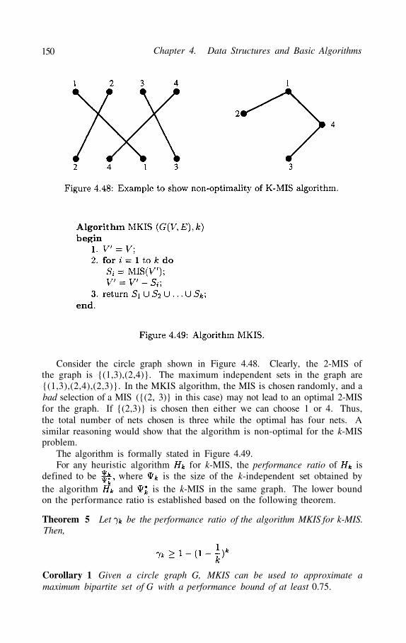
150 Chapter 4. Data Structures and Basic Algorithms
Consider the circle graph shown in Figure 4.48. Clearly, the 2-MIS ofthe graph is {(1,3),(2,4)}. The maximum independent sets in the graph are{(1,3),(2,4),(2,3)}. In the MKIS algorithm, the MIS is chosen randomly, and abad selection of a MIS ({(2, 3)} in this case) may not lead to an optimal 2-MISfor the graph. If {(2,3)} is chosen then either we can choose 1 or 4. Thus,the total number of nets chosen is three while the optimal has four nets. Asimilar reasoning would show that the algorithm is non-optimal for the k-MISproblem.
The algorithm is formally stated in Figure 4.49.For any heuristic algorithm for k-MIS, the performance ratio of is
defined to be where is the size of the k-independent set obtained bythe algorithm and is the k-MIS in the same graph. The lower boundon the performance ratio is established based on the following theorem.
Theorem 5 Let be the performance ratio of the algorithm MKIS for k-MIS.Then,
Corollary 1 Given a circle graph G, MKIS can be used to approximate amaximum bipartite set of G with a performance bound of at least 0.75.

4.6. Summary 151
It is easy to see that the function is a decreasingfunction. Moreover,
where Therefore, we have
Corollary 2 For any integer k, the performance ratio of the algorithm MKISfor k-MIS is at least
Although the approximation result presented above is for circle graphs, thisequally applicable to any class of graphs where the problem of finding MIS ispolynomial time solvable.
Another variation of the MIS problem in circle graphs is called k-densityMIS. Given a set of intervals, the objective of k-density MIS is to find anindependent set of intervals with respect to overlap property such that theinterval graph corresponding to that set has a clique of size at most k.
4.5.6.3 Maximum Clique
Given a circle graph G = (V, E), it is easy to show that for every vertexthe induced subgraph is a permutation graph, where,
For each maximum clique can be found using the algorithm presented formaximum clique in a permutation graph. Let be the maximum clique in
then the maximum clique in G is given by for all It iseasy to see that the time complexity of this algorithm is
4.6 SummaryA VLSI layout is represented as a collection of tiles on several layers. A cir-
cuit may consists of millions of such tiles. Since layout editors are interactive,their underlying data structures should enable editing operations to be per-formed within an acceptable response time. Several data structures have beenproposed for layout systems. The most popular data structure among these iscorner stitch. However, none of the data structures is equally good for all theoperations. The main limitation of all the existing data structures is that theyonly work on rectangular objects. In other words, the data structures do notsupport any other shaped objects such as circular, L-shaped. Therefore, de-velopment of new data structure is needed to handle different shaped objects.

152 Chapter 4. Data Structures and Basic Algorithms
Also, as parallel computation becomes practical, new data structures need tobe developed to adapt to the parallel computation environment.
Due to sheer size of VLSI circuits, low time complexity is necessary foralgorithms to be practical. In addition, due to NP-hardness of many problems,heuristic and approximation algorithms play a very important role in physicaldesign automation.
Several special graphs are used to represent VLSI layouts. The study ofalgorithms of these graphs is essential to development of efficient algorithmsfor various phases in VLSI physical design cycle.
4.7 Exercises
1.
2.
3.
4.
5.
Design an algorithm to insert a block in a given area using the modifiedlinked list data structure. Note that you need to use area searchingoperation to insert a block and a modified linked list to keep track of thevacant tiles.
Design an algorithm to delete a given block from a given set of blocksusing modified linked list data structure. Note that once a block is deletedthe area occupied by that block becomes vacant tile and the linked listmust be updated to take care of this situation.
Design algorithms using a linked list data structure to perform the plow-ing and compaction operations.
Solve the problem 3 using a modified linked list.
The problem of connectivity extraction is very important in circuit ex-traction phase of physical design. It is defined as follows. Given a set ofblocks in an area, let us assume that there isa type associated to each circuit. For example, all the blocks can of onetype and all the vacant tiles could be of another type. Two blocks and
are called connected if there is a sequence of distinct blocksof the same type such that
and is a neighbor of is a neighbor ofand so on and finally is a neighbor of
(a)
(b)
Design an algorithm using a modified linked list data structure toextract the connectivity of two blocks.
Design an algorithm using a corner stitch data structure to find theconnectivity of two blocks.
†6. The existing data structure can be modified to handle layouts in a mul-tilayer environment. Consider the following data items associated to atiles in a multilayer environment:
record Tile =

4.7. Exercises 153
coordinate;height;width;type;text;layer;
end record
(a)
(b)
Design an algorithm to move the entire layout in one direction.
Following problem 5, find the connectivity of any two blocks in amultilayer environment using corner stitch data structure.
7.
8.
Modify algorithm NEIGHBOR-FINDl to find all the neighbors of a givenblock using a linked list data structure.
Modify algorithm NEIGHBOR-FIND2 to find all the neighbors of a givenblock using bin-based data structure.
†9.
10.
11.
12.
Assume a layout system that allows 45° segments, i.e., the blocks couldbe 45° angled parallelogram as well as rectangular. Modify the cornerstitch data structure to handle this layout system. Are four pointers stillsufficient in this situation ?
Given a family of sets of segments where is theset of segments belonging to net on a layer.
Determine if there is a connectivity violation by developing an algorithmwhich finds all such violations.
For the set of intervals shown in Figure 4.50, find maximum independentset, maximum clique, and maximum bipartite subgraph in the intervalgraph defined by the intervals.
For the matching diagram shown in Figure 4.51, find its permutationgraph. Find maximum independent set, minimum number of colors re-quired to color it, and maximum bipartite subgraph in this permutationgraph.

154 Chapter 4. Data Structures and Basic Algorithms
13. For the switchbox shown in Figure 4.52, find maximum independent set,maximum clique, and maximum bipartite subgraph in the permutationgraph defined by the matching diagram.
†14.
†15.
†16.
17.
†18.
19.
Prove that the algorithm MAX-CLIQUE correctly finds the size of themaximum clique in an interval graph.
Improve the time complexity of the algorithm MAX-CLIQUE to O(n log n).The algorithm should also be able to report a maximum clique.
Prove that the algorithm MIS for finding a maximum independent set incircle graphs does indeed find the optimal solution.
Develop a heuristic algorithm for finding a maximum bipartite subgraphin circle graphs.
Implement the approximation algorithm for finding a k-independent set incircle graphs. Experimentally evaluate the performance of the algorithmby implementing an exponential time complexity algorithm for finding ak-independent set.
Develop an efficient algorithm to find a k-density MIS in circle graphs.

4.7. Exercises 155
20.
†21.
22.
23.
†24.
Steiner trees play a key role in global and detail routing problems. Con-sider the following Single Trunk Steiner Tree problem. A single trunkSteiner tree consists of a single horizontal line segment and all the pointsare joined by short vertical line segments. An example of a single trunkSteiner tree is shown in Figure 4.53.
Given a set of n points in a plane, develop an O(n) algorithm for theminimum cost single trunk Steiner tree.
Prove that for n = 3, single trunk Steiner tree is indeed an optimalrectilinear Steiner tree.
For n = 4, give an example which shows that single trunk Steiner tree isnot an optimal rectilinear Steiner tree.
Single trunk Steiner tree can be easily generalized to k-trunk Steinertree problem, which consists of k non-overlapping horizontal trunks. Anexample of a two trunk Steiner tree is shown in Figure 4.54.
Develop an efficient algorithm for 2-trunk Steiner tree problem.
Does there exist an algorithm for the k-trunk Steiner tree problem,for a small constant c?

156 Chapter 4. Data Structures and Basic Algorithms
†25.
†26.
27.
†28.
Implement Hadlock’s Algorithm for finding max-cut in a planar graph.
Prove that Hadlock’s algorithm is optimal by showing it deletes minimumnumber of edges.
Given a set of rectangles in a plane, develop an efficient algorithm todetect if any two rectangles intersect or contain each other.
Given a switch box, develop an efficient algorithm to find the minimumdiameter of rectilinear Steiner trees. The diameter of a tree is the maxi-mum distance between any two of its vertices.
Bibliographic NotesThe paper by John Ousterhout on the corner stitch data structure [Ous84] givesdetails of different algorithms used to manipulate a layout. The corner stitchdata structure has been extended in various ways to account for nonrectilinearshapes and interaction of objects in different layers. In [Meh94] D. P. Mehtapresented a technique for estimating the storage requirements of the Rectan-gular Corner Stitching data structure and the L-shaped Corner Stitching DataStructure on a given circuit by studying the circuit’s geometric properties.
However, there are no efficient data structures to express the true threedimensional nature of a VLSI layout. The details of CIF can be found in Mead& Conway [MC79].
Cormen, Leiserson and Rivest [CLR90], present an in depth analysis ofgraph algorithms. Tarjan [Tar83] provides excellent reference for graph match-ings, minimum spanning trees, and network flow algorithms. Computationalgeometry algorithms are discussed in detail by Preparata and Shamos [PS85].The theory of NP-completeness is discussed in great detail in Garey and John-son [GJ79].
General graph concepts have been described in detail in [CL86]. Algorithmsand concepts for the perfect graphs, interval graphs, permutation graphs, andcircle graphs can be found in [Gol80].