Embed Size (px)
DESCRIPTION
Data Structures – LECTURE 16 All shortest paths algorithms. Properties of all shortest paths Simple algorithm: O (| V | 4 ) time Better algorithm: O (| V | 3 lg | V |) time Floyd-Warshall algorithm: O (| V | 3 ) time Chapter 25 in the textbook (pp 620–635). All shortest paths. - PowerPoint PPT Presentation
Citation preview

Data Structures, Spring 2004 © L. Joskowicz 1
Data Structures – LECTURE 16
All shortest paths algorithms
• Properties of all shortest paths
• Simple algorithm: O(|V|4) time
• Better algorithm: O(|V|3 lg |V|) time
• Floyd-Warshall algorithm: O(|V|3) time
Chapter 25 in the textbook (pp 620–635).

Data Structures, Spring 2004 © L. Joskowicz 2
All shortest paths• Generalization of the single source shortest-path
problem.
• Simple solution: run the shortest path algorithm for each vertex complexity is O(|E|.|V|.|V|) = O(|V|4) for Bellman-Ford and O(|E|.lg |V|.|V|) = O(|V|3 lg |V|) for Dijsktra.
• Can we do better? Intuitively it would seem so, since there is a lot of repeated work exploit the optimal sub-path property.
• We indeed can do better: O(|V|3).
Data Structures, Spring 2004 © L. Joskowicz 3
All-shortest paths: example (1)
2
3 1
5 46
72-4
1
8
3 4
-5

Data Structures, Spring 2004 © L. Joskowicz 4
All-shortest paths: example (2)
2
3 1
5 46
72-4
1
8
3 4
-5
0
1
-3
-4 2
2
3 1
5 46
72-4
1
8
3 4
-5
)42310( 1 2 3 4 5
dist )1543(1 2 3 4 5
pred

Data Structures, Spring 2004 © L. Joskowicz 5
All-shortest paths: example (3)
2
3 1
5 46
72-4
1
8
3 4
-5
0
3 -4
1-1
2
3 1
5 46
72-4
1
8
3 4
-5
)11403( 1 2 3 4 5
dist )1244( 1 2 3 4 5
pred
Data Structures, Spring 2004 © L. Joskowicz 6
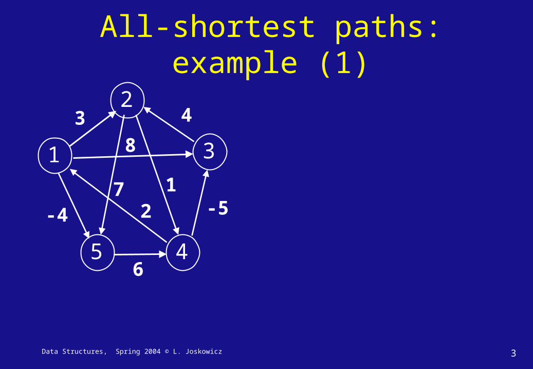
All shortest-paths: representation We will use matrices to represent the graph, the
shortest path lengths, and the predecessor sub-graphs.
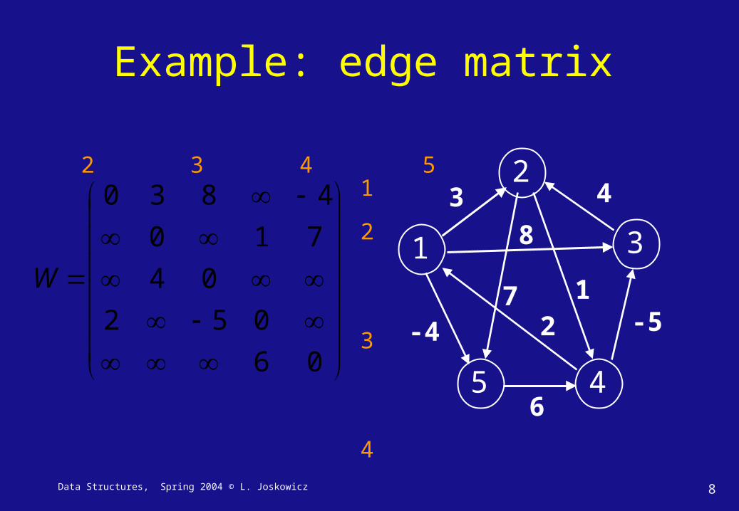
• Edge matrix: entry (i,j) in adjacency matrix W is the weight of the edge between vertex i and vertex j.
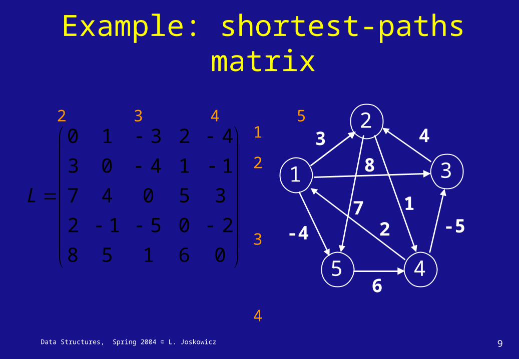
• Shortest-path lengths matrix: entry (i,j) in L is the shortest path length between vertex i and vertex j.
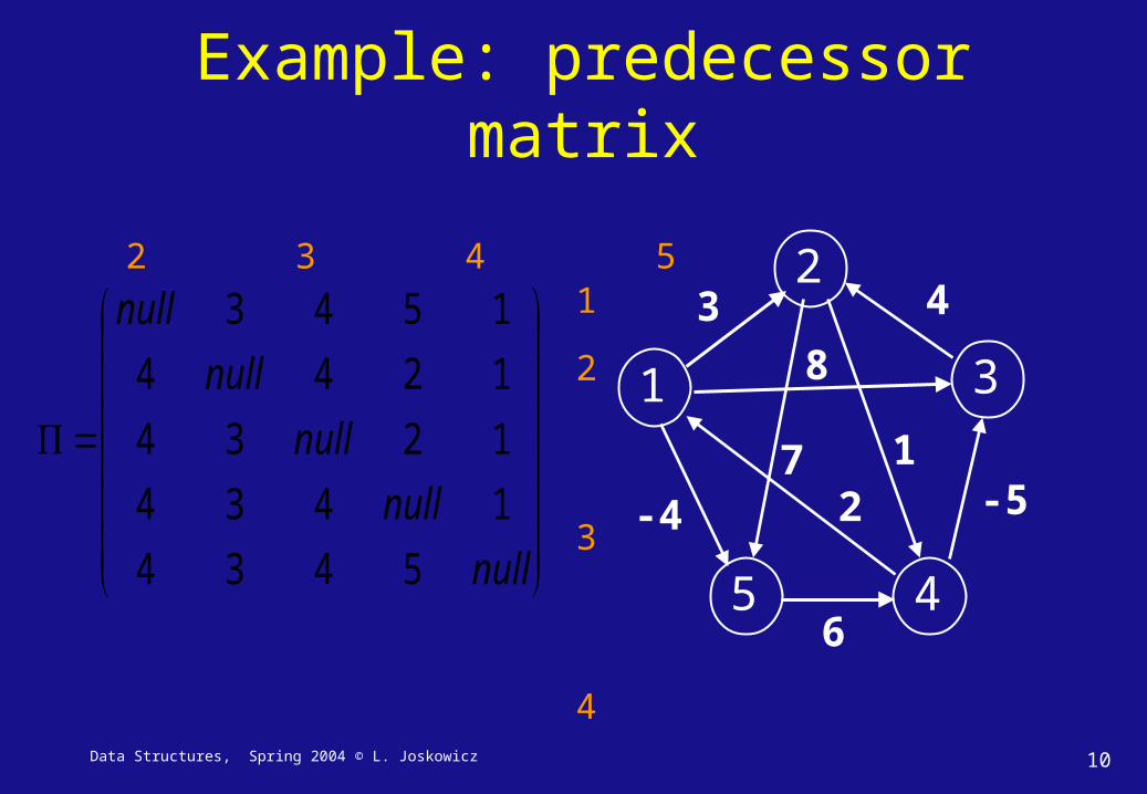
• Predecessor matrix: entry (i,j) in Π is the predecessor of j on some shortest path from i (null when i = j or when there is no path).
Data Structures, Spring 2004 © L. Joskowicz 7
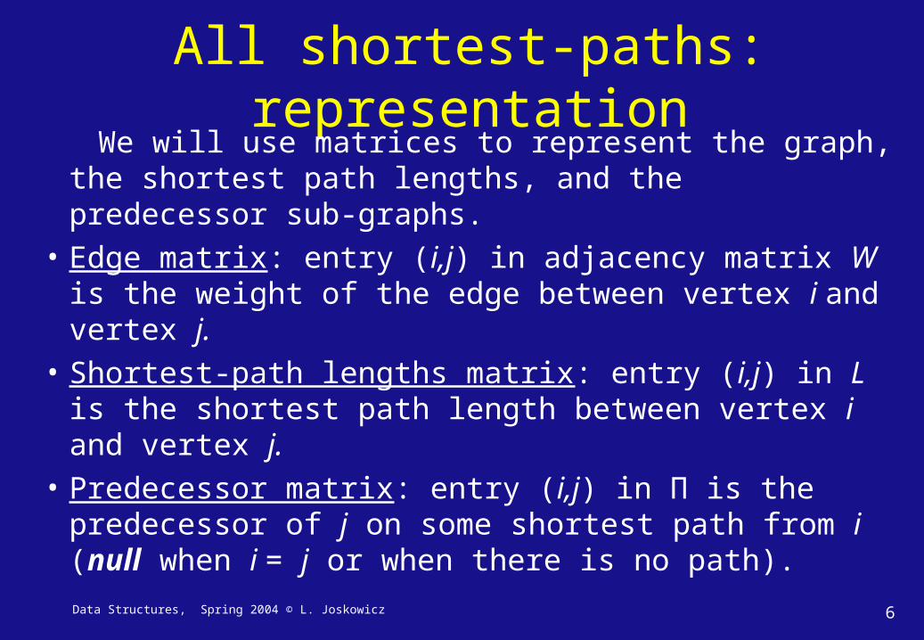
All-shortest paths: definitions
Ejiji
Ejiji
ji
jiwwij
),(and
),(and
if
),(
0
Edge matrix: entry (i,j) in adjacency matrix W
is the weight of the edge between vertex i and vertex j.
Shortest-paths graph: the graphs Gπ,i = (Vπ,i, Eπ,i)
are the shortest-path graphs rooted at vertex I, where:}{}:{, inullVjV iji
}}{:),{( ,, iVjjE iiji
Data Structures, Spring 2004 © L. Joskowicz 8
Example: edge matrix
2
3 1
5 46
72-4
1
8
3 4
-5
06
052
04
710
4830
W
1 2 3 4 51
2
3
4
5
Data Structures, Spring 2004 © L. Joskowicz 9
Example: shortest-paths matrix
2
3 1
5 46
72-4
1
8
3 4
-5
06158
20512
35047
11403
42310
L
1 2 3 4 51
2
3
4
5
Data Structures, Spring 2004 © L. Joskowicz 10
Example: predecessor matrix
2
3 1
5 46
72-4
1
8
3 4
-5
null
null
null
null
null
5434
1434
1234
1244
15431 2 3 4 5
1
2
3
4
5

Data Structures, Spring 2004 © L. Joskowicz 11
The structure of a shortest path1. All sub-paths of a shortest path are shortest paths.
Let p = <v1, .. vk> be the shortest path from v1 to vk. The sub-path between vi and vj, where 1 ≤ i,j ≤ k, pij = <vi, .. vj> is a shortest path.
2. The shortest path from vertex i to vertex j with at most m edges is either:
– the shortest path with at most (m-1) edges (no improvement)
– the shortest path consisting of a shortest path within the (m-1) vertices + the weight of the edge from a vertex within the (m-1) vertices to an extra vertex m.
Data Structures, Spring 2004 © L. Joskowicz 12
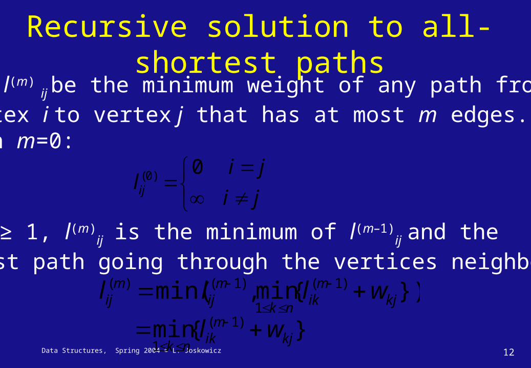
Recursive solution to all-shortest paths
}){min,min( )1(
1
)1()(kj
mik
nk
mij
mij wlll
}{min )1(
1kj
mik
nkwl
ji
jilij
0)0(
Let l(m) ij be the minimum weight of any path from vertex i to vertex j that has at most m edges.When m=0:
For m ≥ 1, l(m)ij is the minimum of l(m–1)
ij and the shortest path going through the vertices neighbors:
Data Structures, Spring 2004 © L. Joskowicz 13
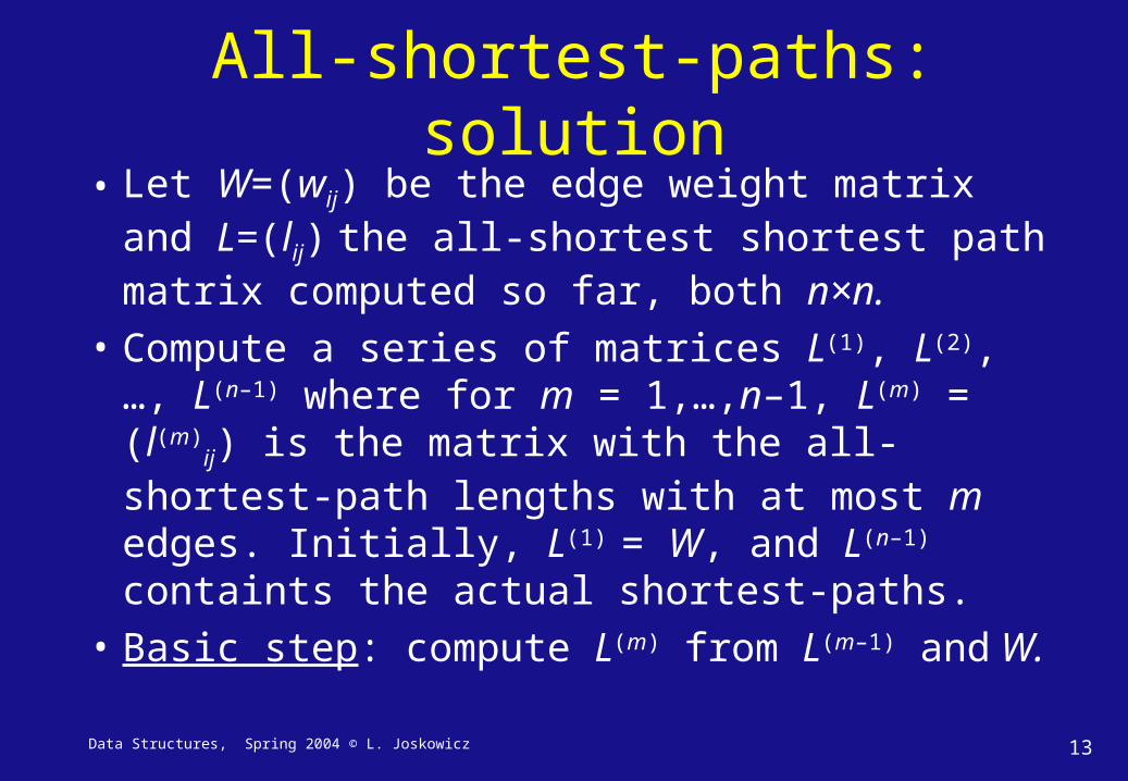
All-shortest-paths: solution
• Let W=(wij) be the edge weight matrix and L=(lij) the all-shortest shortest path matrix computed so far, both n×n.
• Compute a series of matrices L(1), L(2), …, L(n–1) where for m = 1,…,n–1, L(m) = (l(m)
ij) is the matrix with the all-shortest-path lengths with at most m edges. Initially, L(1) = W, and L(n–1) containts the actual shortest-paths.
• Basic step: compute L(m) from L(m–1) and W.

Data Structures, Spring 2004 © L. Joskowicz 14
Algorithm for extending all-shortest paths by one edge: from L(m-1) to L(m)
Extend-Shortest-Paths(L=(lij),W)n rows[L]
Let L’ =(l’ij) be an n×n matrix.for i 1 to n do for j 1 to n do
l’ij ∞ for k 1 to n do
l’ij min(l’ij, lik + wkj)return L’
Complexity: Θ(|V|3)
Data Structures, Spring 2004 © L. Joskowicz 15
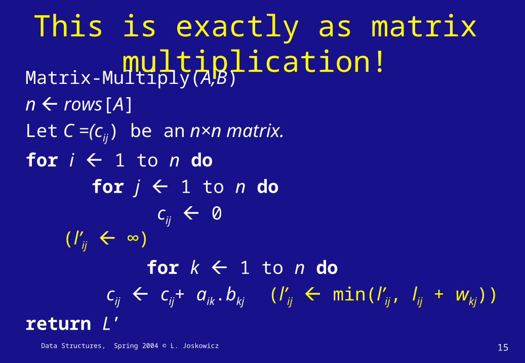
This is exactly as matrix multiplication!Matrix-Multiply(A,B)
n rows[A]
Let C =(cij) be an n×n matrix.
for i 1 to n do
for j 1 to n do
cij 0 (l’ij ∞)
for k 1 to n do
cij cij+ aik.bkj (l’ij min(l’ij, lij + wkj))
return L’
Data Structures, Spring 2004 © L. Joskowicz 16
0618
20512
11504
71403
42830
06
052
04
710
4830
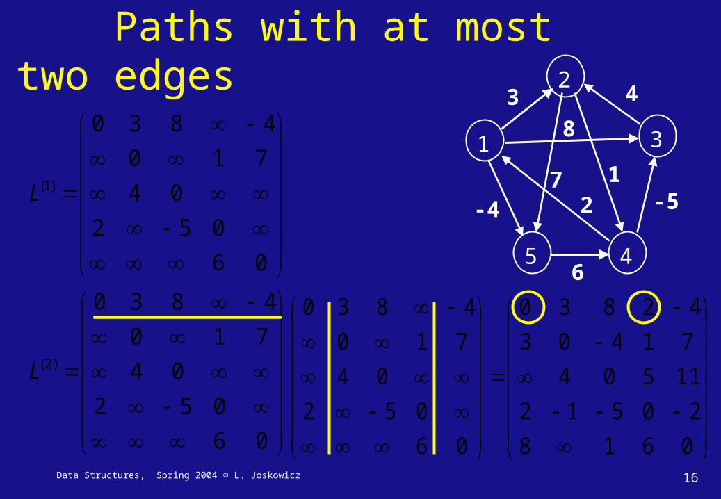
)2(L
Paths with at most two edges
06
052
04
710
4830
)1(L
06
052
04
710
4830
2
3 1
5 46
72-4
1
8
3 4
-5

Data Structures, Spring 2004 © L. Joskowicz 17
Paths with at most three edges
06
052
04
710
4830
06158
20512
115047
11403
42330
2
3 1
5 46
72-4
1
8
3 4
-5
0618
20512
11504
71403
42830
)2(L
0618
20512
11504
71403
42830
)3(L
06158
20512
115047
11403
42330
Data Structures, Spring 2004 © L. Joskowicz 18
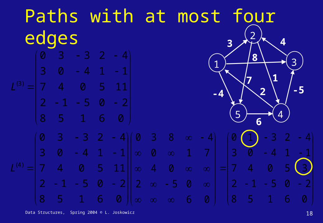
Paths with at most four edges
06158
20512
115047
11403
42330
)3(L
06
052
04
710
4830
2
3 1
5 46
72-4
1
8
3 4
-5
06158
20512
115047
11403
42330
)4(L
06158
20512
35047
11403
42310

Data Structures, Spring 2004 © L. Joskowicz 19
Paths with at most five edges
06158
20512
35047
11403
42310
)4(L
06
052
04
710
4830
2
3 1
5 46
72-4
1
8
3 4
-5
06158
20512
35047
11403
42310
)5(L
06158
20512
35047
11403
42310
Data Structures, Spring 2004 © L. Joskowicz 20
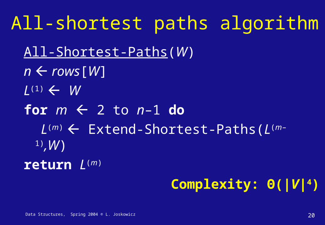
All-shortest paths algorithm
All-Shortest-Paths(W)
n rows[W]
L(1) W
for m 2 to n–1 do
L(m) Extend-Shortest-Paths(L(m–1),W)
return L(m)
Complexity: Θ(|V|4)

Data Structures, Spring 2004 © L. Joskowicz 21
Improved all-shortest paths algorithm• The goal is to compute the final L(n–1), not all the L(m)
• We can avoid computing most L(m) as follows:
L(1) = W
L(2) = W.W
L(4) = W4 = W2.W2
… )12()12()2()2( )1lg()1lg()1lg()1lg(
.
nnnn
WWWL
Since the final product is equal to L(n–1) 12 )1lg( nn
only |lg(n–1)| iterations are necessary!
repeated squaring
Data Structures, Spring 2004 © L. Joskowicz 22
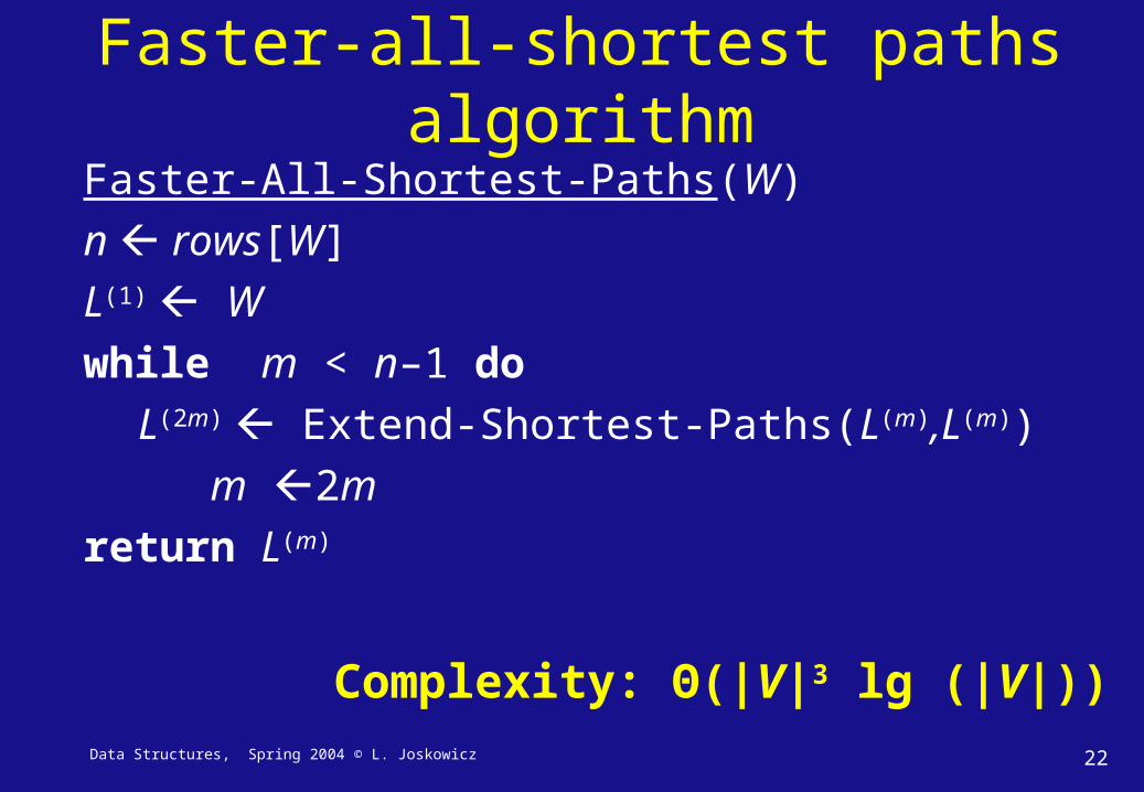
Faster-all-shortest paths algorithm
Faster-All-Shortest-Paths(W)
n rows[W]
L(1) W
while m < n–1 do
L(2m) Extend-Shortest-Paths(L(m),L(m))
m 2m
return L(m)
Complexity: Θ(|V|3 lg (|V|))

Data Structures, Spring 2004 © L. Joskowicz 23
Floyd-Warshall algorithm
• Assumes there are no negative-weight cycles.
• Uses a different characterization of the structure of the shortest path. It exploits the properties of the intermediate vertices of the shortest path.
• Runs in O(|V|3).

Data Structures, Spring 2004 © L. Joskowicz 24
Structure of the shortest path (1)• An intermediate vertex vi of a simple path p=<v1,..,vk>
is any vertex other than v1 or vk.
• Let V={1,2,…,n} and let K={1,2,…,k} be a subset for k ≤ n. For any pair of vertices i,j in V, consider all paths from i to j whose intermediate vertices are drawn from K. Let p be the minimum-weight path among them.
ik1
j
k2
p
Data Structures, Spring 2004 © L. Joskowicz 25
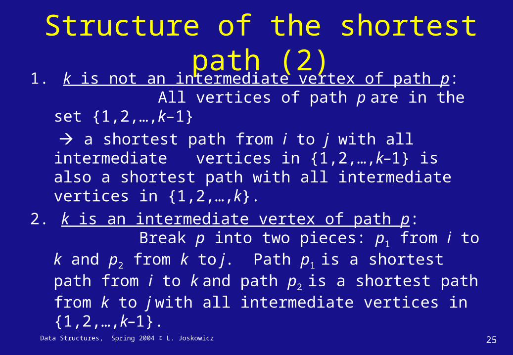
Structure of the shortest path (2)1. k is not an intermediate vertex of path p:
All vertices of path p are in the set {1,2,…,k–1}
a shortest path from i to j with all intermediate vertices in {1,2,…,k–1} is also a shortest path with all intermediate vertices in {1,2,…,k}.
2. k is an intermediate vertex of path p: Break p into two pieces: p1 from i to k and p2 from k to j. Path p1 is a shortest path from i to k and path p2 is a shortest path from k to j with all intermediate vertices in {1,2,…,k–1}.
Data Structures, Spring 2004 © L. Joskowicz 26
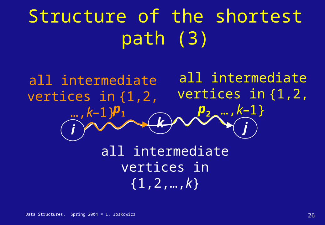
Structure of the shortest path (3)
i k j
p2
all intermediate vertices in {1,2,…,k–1}
all intermediate vertices in {1,2,…,k}
p1
all intermediate vertices in {1,2,…,k–1}
Data Structures, Spring 2004 © L. Joskowicz 27
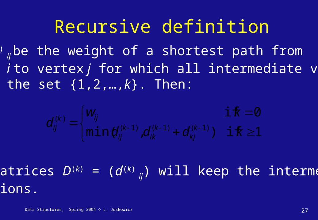
Recursive definition
1if),min(
0if)1()1()1(
)(
kddd
kwd k
kjk
ikk
ij
ijkij
Let d(k) ij be the weight of a shortest path from vertex i to vertex j for which all intermediate verticesare in the set {1,2,…,k}. Then:
The matrices D(k) = (d(k) ij) will keep the intermediatesolutions.
Data Structures, Spring 2004 © L. Joskowicz 28
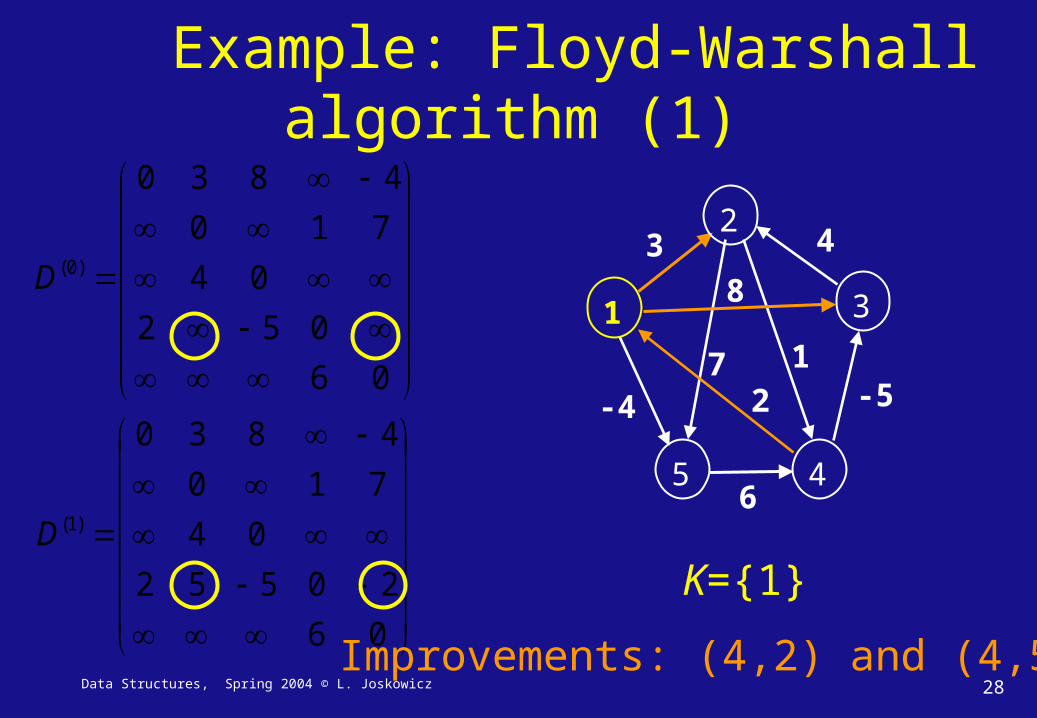
Example: Floyd-Warshall algorithm (1)
06
052
04
710
4830
)0(D
06
20552
04
710
4830
)1(D
2
3 1
5 46
72-4
1
8
3 4
-5
K={1}
Improvements: (4,2) and (4,5)
Data Structures, Spring 2004 © L. Joskowicz 29
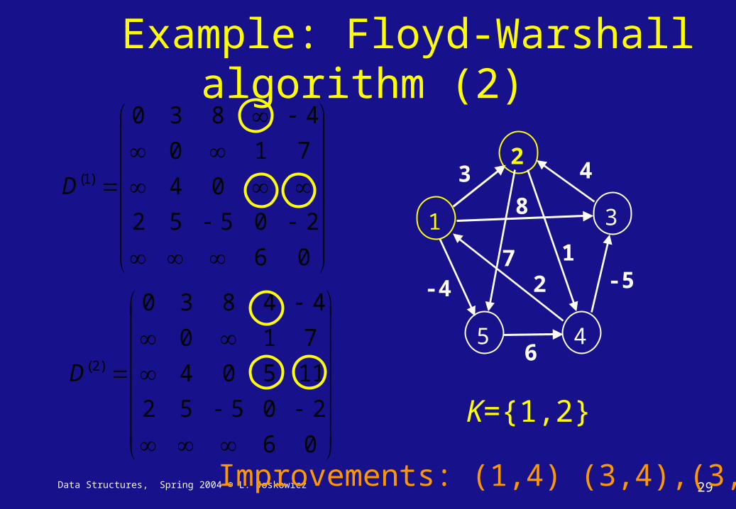
Example: Floyd-Warshall algorithm (2)
06
20552
11504
710
44830
)2(D
06
20552
04
710
4830
)1(D 2
3 1
5 46
72-4
1
8
3 4
-5
K={1,2}
Improvements: (1,4) (3,4),(3,5)
Data Structures, Spring 2004 © L. Joskowicz 30
06
20552
11504
710
44830
)2(D
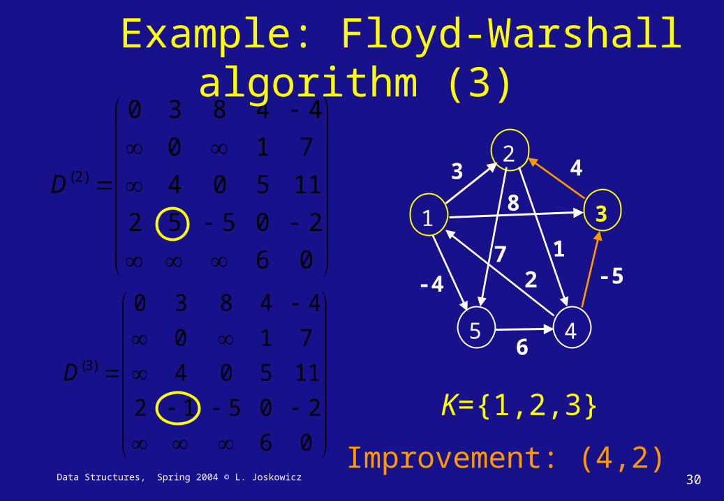
Example: Floyd-Warshall algorithm (3)
06
20512
11504
710
44830
)3(D
2
3 1
5 46
72-4
1
8
3 4
-5
K={1,2,3}
Improvement: (4,2)

Data Structures, Spring 2004 © L. Joskowicz 31
06158
20512
35047
11403
44130
)4(D
Example: Floyd-Warshall algorithm (4)
06
20512
11504
710
4830
)3(D
2
3 1
5 46
72-4
1
8
3 4
-5
K={1,2,3,4}
Improvements: (1,3),(1,4) (2,1), (2,3), (2,5)(3,1),(3,5), (5,1),(5,2),(5,3)
Data Structures, Spring 2004 © L. Joskowicz 32
06158
20512
35047
11403
44130
)4(D
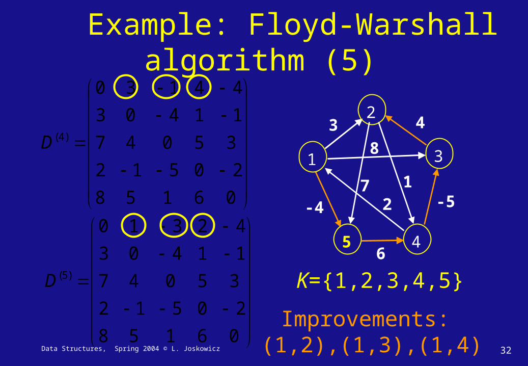
Example: Floyd-Warshall algorithm (5)
06158
20512
35047
11403
42310
)5(D
2
3 1
5 46
72-4
1
8
3 4
-5
K={1,2,3,4,5}
Improvements: (1,2),(1,3),(1,4)

Data Structures, Spring 2004 © L. Joskowicz 33
Transitive closure (1)• Given a directed graph G=(V,E) with vertices
V = {1,2,…,n} determine for every pair of vertices (i,j) if there is a path between them.
• The transitive closure graph of G, G*=(V,E*) is such that E* = {(i,j): if there is a path i and j}.
• Represent E* as a binary matrix and perform logical binary operations AND (/\) and OR (\/) instead of min and + in the Floyd-Warshall algorithm.

Data Structures, Spring 2004 © L. Joskowicz 34
Transitive closure (2)
0for
),( and0if
),( and0if
)/\(/\
1
0
)1()1()1(
)(
k
Ejik
Ejik
ttt
tk
kjk
ikk
ij
kij
The definition of the transitive closure is:
The matrices T(k) indicate if there is a path withat most k edges between s and i.
Data Structures, Spring 2004 © L. Joskowicz 35
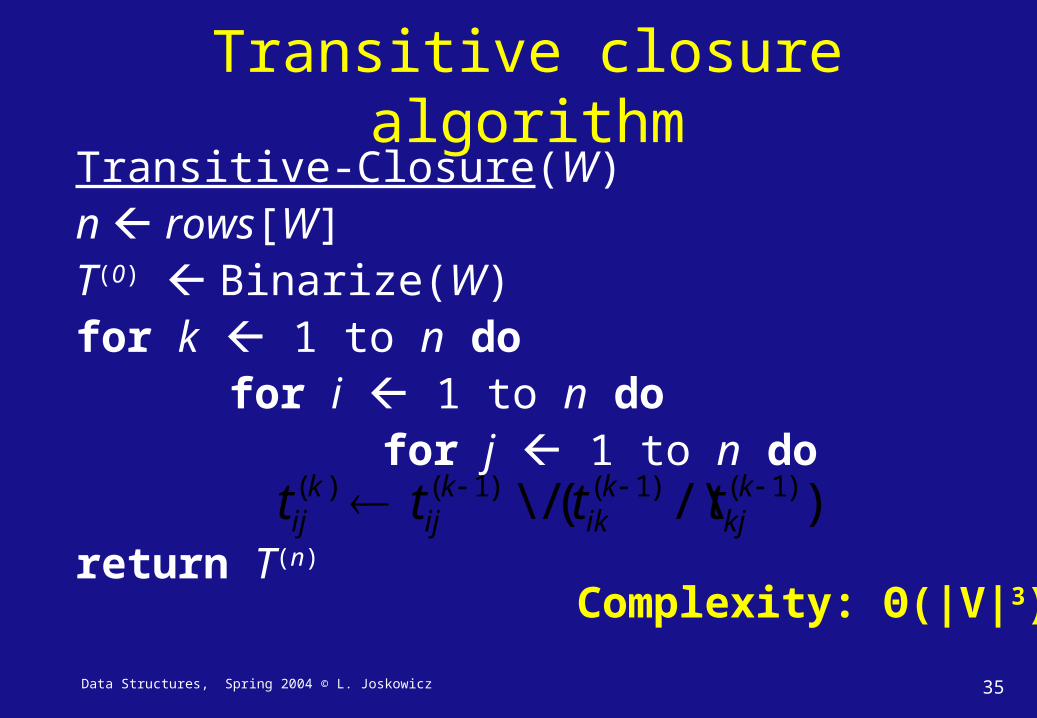
Transitive closure algorithmTransitive-Closure(W)n rows[W] T(0) Binarize(W)for k 1 to n do for i 1 to n do for j 1 to n do return T(n)
Complexity: Θ(|V|3)
)/\(/\ )1()1()1()( kkj
kik
kij
kij tttt
Data Structures, Spring 2004 © L. Joskowicz 36
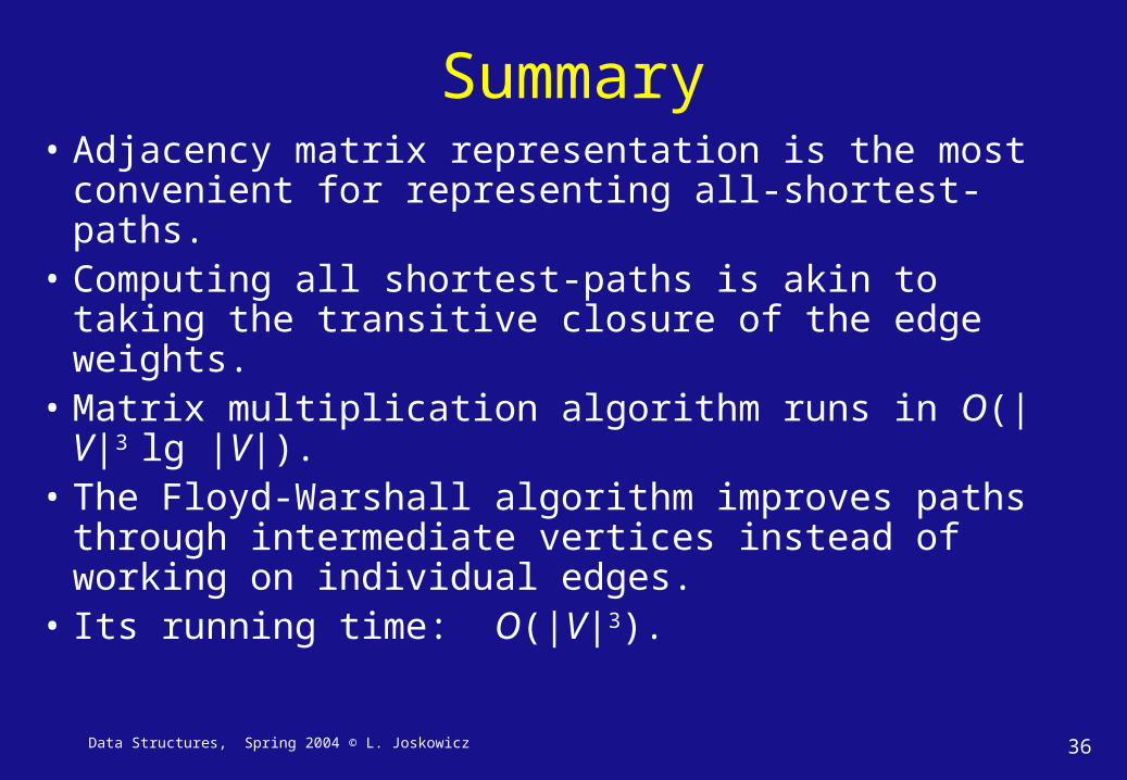
Summary• Adjacency matrix representation is the most
convenient for representing all-shortest-paths.• Computing all shortest-paths is akin to taking the
transitive closure of the edge weights.• Matrix multiplication algorithm runs in O(|V|3 lg |V|).• The Floyd-Warshall algorithm improves paths
through intermediate vertices instead of working on individual edges.
• Its running time: O(|V|3).

Data Structures, Spring 2004 © L. Joskowicz 37
Other graph algorithms• Many more interesting problems, including
network flow, graph isomorphism, coloring, partition, etc.
• Problems can be classified by the type of solution.• Easy problems: polynomial-time solutions O(f (n))
where f (n) is a polynomial function of degree at most k.
• Hard problems: exponential-time solutions O(f (n)) where f (n) is an exponential function, usually 2n.
Data Structures, Spring 2004 © L. Joskowicz 38
Easy graph problems
• Network flow – maximum flow problem
• Maximum bipartite matching
• Planarity testing and plane embedding.
Data Structures, Spring 2004 © L. Joskowicz 39
Hard graph problems• Graph and sub-graph isomorphism.
• Largest clique, Independent set
• Vertex tour (Traveling Salesman problem)
• Graph partition
• Vertex coloring
However, not all is lost!
• Good heuristics that perform well in most cases
• Polynomial-time approximation algorithms