Embed Size (px)
Citation preview

DATA STRUCTURES + SORTING + STRING COMP 321 – McGill University These slides are mainly compiled from the following resources.
- Professor Jaehyun Park’ slides CS 97SI - Top-coder tutorials. - Programming Challenges book.

Comments • Urgent => https://open.kattis.com/ • Contest Saturday VS ICPC. • No details => Go over the topics on weekend. • No overstress – No overconfident.

Data Structure • A way to store and organize data in order to support
efficient insertions, queries, searches, updates, and deletions.

Data Structure • Basic data structures (built-in libraries).
• Linear DS. • Non-Linear DS.
• Data structures (Own libraries). • Graphs. • Union-Find Structures. • Segment Tree.

Data Structures • Basic data structures (built-in libraries).
• Linear DS (ordering the elements sequentially). • Static Array (Array in C/C++ and in Java). • Resizeable array (C++ STL<vector> and Java ArrayList). • Linked List: (C++ STL<list> and Java LinkedList). • Stack (C++ STL<stack> and Java Stack). • Queue (C++ STL <queue> and Java Queue).

Data Structures • Basic data structures (built-in libraries).
• Non-Linear DS. • Balanced Binary Search Tree (C++ STL <map>/<set> and in Java
TreeMap/TreeSet). • AVL and Red-Black Trees = Balanced BST • <map> stores (key -> data) VS <set> only stores the key
• Heap(C++ STL<queue>:priority_queue and Java PriorityQueue). • BST complete. • Heap property VS BST protperty.
• Hash Table (Java HashMap/HashSet/HashTable). • Non synchronized vs synchronized. • Null vs non-nulls • Predictable iteration vs non predictable.

Question for you. • Basic data structures (built-in libraries).
• Non Linear DS (non-sequential ordering). • Balanced Binary Search Tree (C++ STL <map>/<set> and Java
TreeMap/TreeSet) • AVL Tree and Red-Black = Balanced BST. • <map> stores (key -> data) VS <set> only stores the key
• Heap (C++ STL <queue> and Java PriorityQueue) • Heap property VS BST property. • Complete BST.
• Hash table
BST HEAP

Deciding the Order of the Tasks • Returns the newest task (stack) • Returns the oldest task (queue) • Returns the most urgent task (priority queue) • Returns the easiest task (priority queue)

STACK • Last in, first out (Last In First Out) • Stacks model piles of objects (such as dinner plates) • Supports three constant-time operations
• Push(x): inserts x into the stack • Pop(): removes the newest item • Top(): returns the newest item
• Very easy to implement using an array

STACK • Have a large enough array s[] and a counter k, which
starts at zero • Push(x) : set s[k] = x and increment k by 1 • Pop() : decrement k by 1 • Top() : returns s[k - 1] (error if k is zero)
• C++ and Java have implementations of stack • stack (C++), Stack (Java)
STACK • Useful for:
• Processing nested formulas • Depth-first graph traversal • Data storage in recursive algorithms

QUEUE • First in, first out (FIFO) • Supports three constant-time operations
• Enqueue(x) : inserts x into the queue • Dequeue() : removes the oldest item • Front() : returns the oldest item
• Implementation is similar to that of stack

QUEUE • Assume that you know the total number of elements that
enter the queue • ... which allows you to use an array for implementation • … If not, you can use linked lists or double linked lists
• Maintain two indices head and tail • Dequeue() increments head • Enqueue() increments tail • Use the value of tail - head to check emptiness
• You can use queue (C++) and Queue (Java)

QUEUE • Useful for
• implementing buffers • simulating waiting lists • shuffling cards
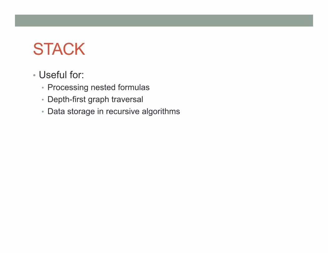
PRIORITY QUEUE • Each element in a PQ has a priority value • Three operations:
• Insert(x, p) : inserts x into the PQ, whose priority is p • RemoveTop() : removes the element with the highest priority • Top() : returns the element with the highest priority
• All operations can be done quickly if implemented using a heap (if not use a sorted array)
• priority_queue (C++), PriorityQueue (Java) • Useful for
• Maintaining schedules / calendars • Simulating events • Sweepline geometric algorithms

HEAP • Complete binary tree with the heap property:
• The value of a node ≥ values of its children • What is the difference between full vs complete?
• The root node has the maximum value • Constant-time top() operation
• Inserting/removing a node can be done in O(log n) time without breaking the heap property • May need rearrangement of some nodes

HEAP
• Start from the root, number the nodes 1, 2, . . . from left to right
• Given a node k easy to compute the indices of its parent and children • Parent node: floor(k/2) • Children: 2k, 2k + 1

Heap – Inserting a Node • 1. Make a new node in the last level, as far left as
possible • If the last level is full, make a new one
• 2. If the new node breaks the heap property, swap with its parent node • The new node moves up the tree, which may introduce another
conflict
• Repeat 2 until all conflicts are resolved • Running time = tree height = O(log n)

Heap – Deleting a Node • 1. Remove the root, and bring the last node (rightmost
node in the last level) to the root • 2. If the root breaks the heap property, look at its children
and swap it with the larger one • Swapping can introduce another conflict
• 3 Repeat 2 until all conflicts are resolved • Running time = O(log n)

BINARY SEARCH TREE (BST) • The idea behind is that each node has, at most, two
children • A binary tree with the following property: for each node v,
• value of v ≥ values in v ’s left subtree • value of v < values in v ’s right subtree

BST • Supports three operations
• Insert(x) : inserts a node with value x • Delete(x) : deletes a node with value x , if there is any • Find(x) : returns the node with value x , if there is any
• Many extensions are possible • Count(x) : counts the number of nodes with value less than or
equal to x • GetNext(x) : returns the smallest node with value ≥ x
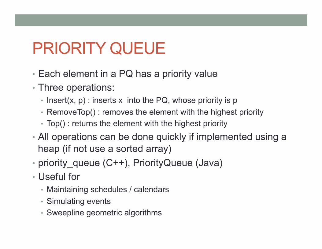
BST • Simple implementation cannot guarantee efficiency
• In worst case, tree height becomes n (which makes BST useless)
• Guaranteeing O(log n) running time per operation requires balancing of the tree (hard to implement). • For example AVL and Red-Black trees (We will skip the details of these
balanced trees, but you should be review it.). • What does balanced mean??
• Use the standard library implementations • set, map (C++) • TreeSet, TreeMap (Java)
BST • Simple implementation cannot guarantee efficiency
• In worst case, tree height becomes n (which makes BST useless)
• Guaranteeing O(log n) running time per operation requires balancing of the tree (hard to implement). • For example AVL and Red-Black trees (We will skip the details of these
balanced trees, but you should be review it.). • What does balanced mean??=> The heights of the two child subtrees of
anny node differ by at most one.
• Use the standard library implementations • set, map (C++) • TreeSet, TreeMap (Java)

Question for you • Why a binary tree is preferable to an array of values that
has been sorted? • O(?) Finding a given key?

Question for you • Why a binary tree is preferable to an array of values that
has been sorted? • O(log n) to find a given key => traversing BST and binary search. • Problem is the adding of a new item.
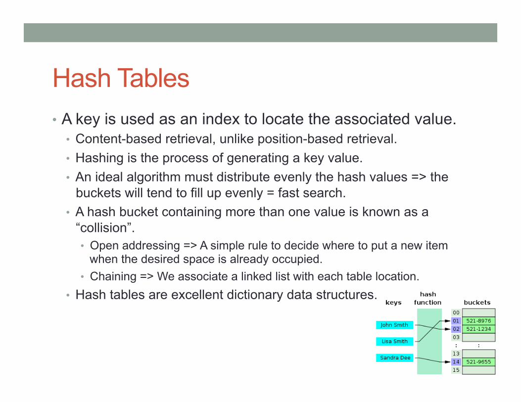
Hash Tables • A key is used as an index to locate the associated value.
• Content-based retrieval, unlike position-based retrieval. • Hashing is the process of generating a key value. • An ideal algorithm must distribute evenly the hash values => the
buckets will tend to fill up evenly = fast search. • A hash bucket containing more than one value is known as a
“collision”. • Open addressing => A simple rule to decide where to put a new item
when the desired space is already occupied. • Chaining => We associate a linked list with each table location.
• Hash tables are excellent dictionary data structures.
Hash Function • A function that takes a string and outputs a number
• A good hash function has few collisions • i.e. , If x != y , H(x) != H(y) with high probability
• An easy and powerful hash function is a polynomial mod some prime p. • Consider each letter as a number (ASCII value is fine) • H(x1 . . . xk) = x1ak−1 + x2ak−2 + . . . + xk−1a + xk (mod p)

Data Structures • Data structures (Own Libraries).
• Graph. • Lets talk about graphs later.
• Union-Find Disjoint Sets • Segment tree.

Union-Find Structure • Used to store disjoint sets
• What is a disjoint set?
• Can support two types of operations efficiently • Find(x) : returns the “representative” of the set that x belongs • Union(x, y) : merges two sets that contain x and y
• Both operations can be done in (essentially) constant time • Super-short implementation! • Useful for problems involving partitioning.
• Ex: keeping track of connected components. • Kruskal’s algorithm (minimum spaning tree).
Union-Find Structure • Used to store disjoint sets
• What is a disjoint set? => sets whose intersection is the empty set.
• Can support two types of operations efficiently • Find(x) : returns the “representative” of the set that x belongs • Union(x, y) : merges two sets that contain x and y
• Both operations can be done in (essentially) constant time • Super-short implementation! • Useful for problems involving partitioning.
• Ex: keeping track of connected components. • Kruskal’s algorithm (minimum spaning tree).

Union-Find Structure • Main idea: represent each set by a rooted tree
• Every node maintains a link to its parent • A root node is the “representative” of the corresponding set • Example: two sets {x, y, z} and {a, b, c, d}

Union-Find Structure • Find(x): follow the links from x until a node points itself
• This can take O(n) time but we will make it faster
• Union(x, y): run Find(x) and Find(y) to find corresponding root nodes and direct one to the other.
• If we assume that the links are stored in L[], then

Union-Find Structure • In a bad case, the trees can become too deep
• ... which slows down future operations
• Path compression makes the trees shallower every time Find() is called.
• We don’t care how a tree looks like as long as the root stays the same • After Find(x) returns the root, backtrack to x and reroute all the
links to the root

Question for you • How can you implement the operation isSameSet(i,j)?

Question for you • How can you implement the operation isSameSet(i,j)?
• simply calls findSet(i) and findSet(j) to check if both refer to the same representative.

Segment Tree • DS to efficiently answer dynamic range queries.
• Range Minimum Query (RMQ): finding the index of the minimum element in an array given a range: [i..j]. • Ex. RMQ(1, 3) = 2, RMQ(3, 4) = 4, RMQ(0, 0) = 0, RMQ(0, 1) = 1, and
RMQ(0, 6) = 5. • Iterate takes O(n), let make it faster using a binary tree similar to heap,
but usually not a complete binary tree (aka segment tree).

Segment Tree • Binary tree. • Each node is associated with some interval of the array. • Each non-leaf node has two children whose associated
intervals are disjoint. • Each child’s interval has approximately half the size of the
parent’s interval.

Segment Tree
• Root => [0, N – 1] and for each segment [l,r] we split them into [l, (l + r) / 2] and [(l + r) / 2 + 1, r] until l = r.

Question for you • What is the complexity of built_segment_tree O(?)? • With segment tree ready, what is the complexity of
answering an RMQ? • Can you give the worst case? RMQ(?,?)
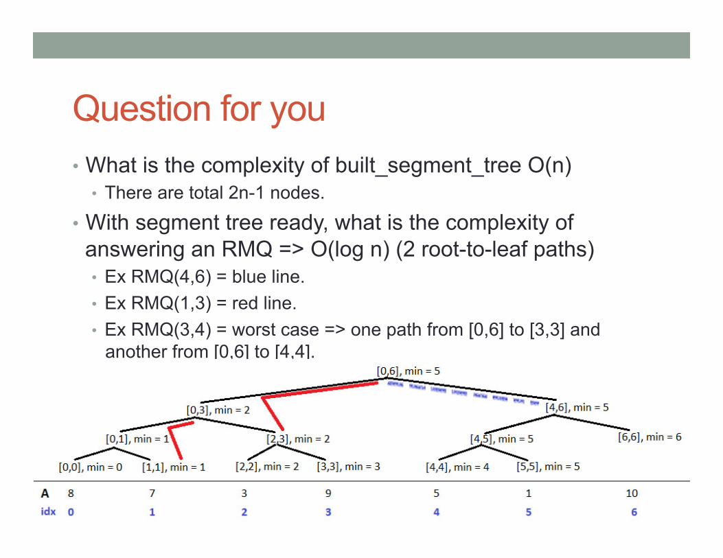
Question for you • What is the complexity of built_segment_tree O(n)
• There are total 2n-1 nodes.
• With segment tree ready, what is the complexity of answering an RMQ => O(log n) (2 root-to-leaf paths) • Ex RMQ(4,6) = blue line. • Ex RMQ(1,3) = red line. • Ex RMQ(3,4) = worst case => one path from [0,6] to [3,3] and
another from [0,6] to [4,4].

Segment Tree • If the array A is static, then use a Dynamic Programming
solution that requires O(nlogn) pre-processing and O(1) per RMQ. • Segment tree becomes useful if array A is frequently updated.
• Ex. Updating A[5] takes O(logn) vs O(nlogn) required by DP.

Fenwick Tree • Full binary tree with at least n leaf nodes
• We will use n = 8 for our example
• kth leaf node stores the value of item k • Each internal node stores the sum of values of its children
• e.g. , Red node stores item[5] + item[6]

Summing Consecutive Values • Main idea: choose the minimal set of nodes whose sum
gives the desired value • at most 1 node is chosen at each level so that the total number of
nodes we look at is log2 n • and this can be done in O(log n) time

Summing Consecutive Values • Sum(7) = sum of the values of gold-colored nodes.

Summing Consecutive Values • Sum(8) = sum of the values of gold-colored nodes.

Summing Consecutive Values • Sum(6) = sum of the values of gold-colored nodes.

Summing Consecutive Values • Sum(3) = sum of the values of gold-colored nodes.

Summing Consecutive Values • Say we want to compute Sum(k)
• Maintain a pointer P which initially points at leaf k • Climb the tree using the following procedure:
• If P is pointing to a left child of some node: • Add the value of P • Set P to the parent node of P’s left neighbor • If P has no left neighbor, terminate
• Otherwise: • Set P to the parent node of P
• Use an array to implement

Updating a Value • Say we want to do Set(k, x) (set the value of leaf k as x)
• 1. Start at leaf k, change its value to x • 2. Go to its parent, and recompute its value • 3. Repeat 2 until the root

SORTING • Practical applications in computing require things to be in
order. • To consider:
• Runtime. • Memory Space.
• In-place algorithms ??? • Stability.
• What happens to elements that are comparatively the same?

SORTING • Practical applications in computing require things to be in
order. • To consider:
• Runtime. • Memory Space.
• In-place algorithms => without creating copies of the data • Stability.
• What happens to elements that are comparatively the same? • Those elements whose comparison key is the same will remain in the
same relative order after sorting as they were before sorting.
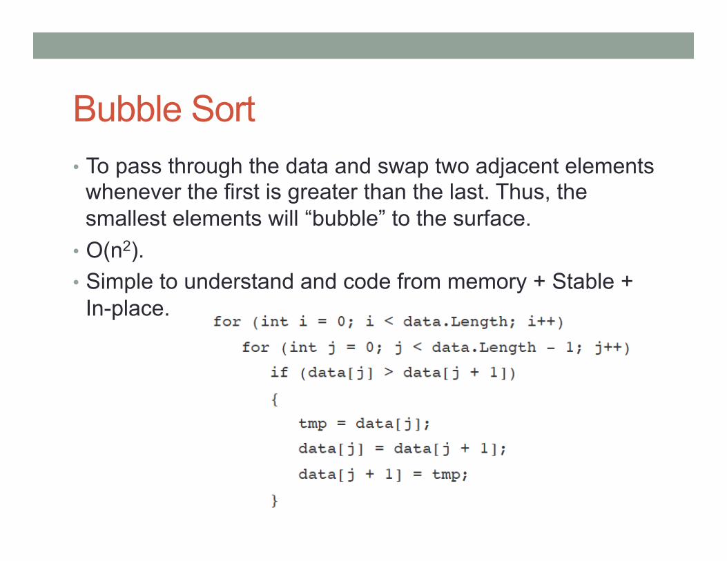
Bubble Sort • To pass through the data and swap two adjacent elements
whenever the first is greater than the last. Thus, the smallest elements will “bubble” to the surface.
• O(n2). • Simple to understand and code from memory + Stable +
In-place.
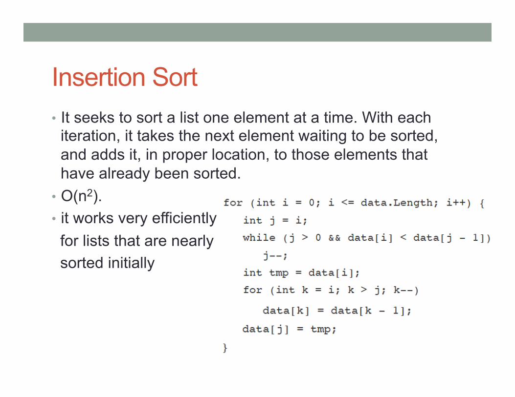
Insertion Sort • It seeks to sort a list one element at a time. With each
iteration, it takes the next element waiting to be sorted, and adds it, in proper location, to those elements that have already been sorted.
• O(n2). • it works very efficiently for lists that are nearly sorted initially

Merge Sort • A merge sort works recursively (divide and conquer).
Divide the unsorted list into n sublists, each containing 1 element. Then, merge sublists to produce new sorted sublists.
• O(n log n). • Faily efficient + can be used to solve other problems.

Heap Sort • All data from a list is inserted into a heap, and then the
root element is repeatedly removed and stored back into the list.
• O(nlogn) • Not stable

Quick Sort • Divide the data into two groups of “high” values and “low”
values. Then, recursively process the two halves. Finally, reassemble the now sorted list.
• O(n2) • dependent upon how successfully an accurate midpoint value is selected

Radix Sort • Sort data without having to directly compare elements to
each other. It groups keys by the individual digits which share the same significant position and value.
• O(n * k), where k is the size of the key. • Some types of data may use very long keys, or may not
easily lend itself to a representation that can be processed

Sorting Libraries • Java API, and C++ STL all provide some built-in sorting
capabilities. • Check the interface called Comparable => you add a
method int CompareTo (object other), which returns a negative value if less than, 0 if equal to, or a positive value if greater than the parameter.
• Also check the interface called Comparator. which defines a single method int Compare (object obj1, object obj2), which returns a value indicating the results of comparing the two parameters.

STRINGS

String Matching Problem • Given a text T and a pattern P, find all occurrences of P
within T • Notations:
• n and m : lengths of P and T • : set of alphabets (of constant size) • Pi : i th letter of P (1-indexed) • a , b , c : single letters in • x , y , z : strings

String Matching Problem • T = AGCATGCTGCAGTCATGCTTAGGCTA • P = GCT • P appears three times in T • A naive method takes O(mn) time
• Initiate string comparison at every starting point • Each comparison takes O(m) time
• We can do much better!

String Matching Problem - Hash • Main idea: preprocess T to speedup queries
• Hash every substring of length k • k is a small constant
• For each query P, hash the first k letters of P to retrieve all the occurrences of it within T
• Don’t forget to check collisions!

String Matching Problem - Hash • Pros:
• Easy to implement • Significant speedup in practice
• Cons: • Doesn’t help the asymptotic efficiency
• Can still take O(nm) time if hashing is terrible or data is difficult • Can you give me an example of the worst case?
• A lot of memory consumption

String Matching Problem - Hash • Pros:
• Easy to implement • Significant speedup in practice
• Cons: • Doesn’t help the asymptotic efficiency
• Can still take O(nm) time if hashing is terrible or data is difficult • Can you give me an example of the worst case? => When all the
characters of pattern and text are same. T=AAAAAAA… P=AAA.
• A lot of memory consumption

SMP - Knuth-Morris-Pratt (KMP) • A linear time (!) algorithm that solves the string matching
problem by preprocessing P in O(m) time • Main idea is to skip some comparisons by using the previous
comparison result.
• Uses an auxiliary array π that is defined as the following: • π[i] is the largest integer smaller than i such that P1 . . . Pπ [i] is a
suffix of P1 . . . Pi • e.g., π[6] = 4 since abab is a suffix of ababab • e.g., π[9] = 0 since no prefix of length ≤ 8 ends with c

Question for you • Why is π useful?

SMP - Knuth-Morris-Pratt (KMP) • T = ABC ABCDAB ABCDABCDABDE • P = ABCDABD • π = (0,0,0,0,1,2,0) • Start matching at the first position of T:
• Mismatch at the 4th letter of P!
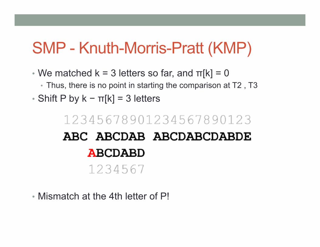
SMP - Knuth-Morris-Pratt (KMP) • We matched k = 3 letters so far, and π[k] = 0
• Thus, there is no point in starting the comparison at T2 , T3
• Shift P by k − π[k] = 3 letters
• Mismatch at the 4th letter of P!

SMP - Knuth-Morris-Pratt (KMP) • We matched k = 0 letters so far • Shift P by k−π[k] = 1 letter (we define π[0] = −1)
• Mismatch at T11!

SMP - Knuth-Morris-Pratt (KMP) • π[6] = 2 means P1P2 is a suffix of P1 . . . P6
• Shift P by 6 − π[6] = 4 letters
• Again, no point in shifting P by 1, 2, or 3 letters

SMP - Knuth-Morris-Pratt (KMP) • Mismatch at T11 again!
• Currently 2 letters are matched • Shift P by 2 − π[2] = 2 letters

SMP - Knuth-Morris-Pratt (KMP) • Mismatch at T11 again!
• Currently no letters are matched • Shift P by 0 − π[0] = 1 letter

SMP - Knuth-Morris-Pratt (KMP) • Mismatch at T18
• Currently 6 letters are matched • Shift P by 6 − π[6] = 4 letters
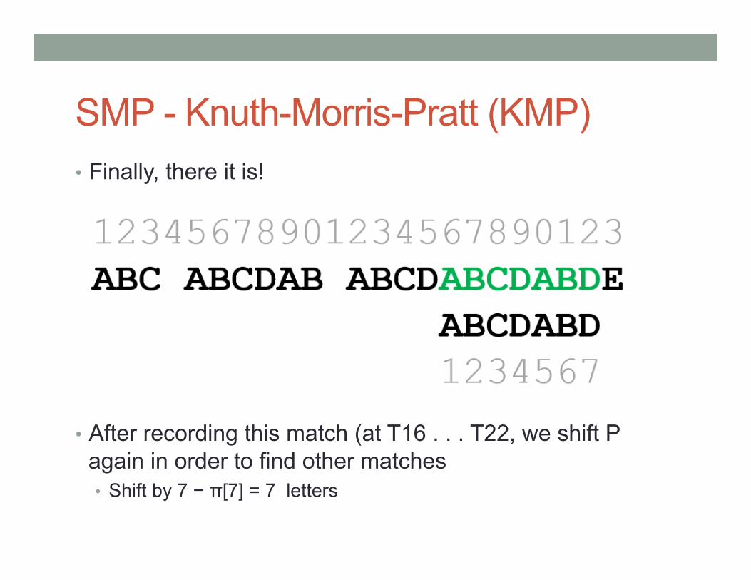
SMP - Knuth-Morris-Pratt (KMP) • Finally, there it is!
• Currently all 7 letters are matched • After recording this match (at T16 . . . T22, we shift P
again in order to find other matches • Shift by 7 − π[7] = 7 letters

SMP - Knuth-Morris-Pratt (KMP) • Computing π. • Obs1=> if P1 . . . Pπ[i] is a suffix of P1 . . . Pi, then P1 . . .
Pπ[i]-1 is a suffix of P1 . . . Pi−1
• Obs2 => all the prefixes of P that are a suffix of P1 . . . Pi can be obtained by recursively applying to I • e.g. , P1 . . . Pπ[i] , P1 . . . , Pπ[π[i]] , P1 . . . , , Pπ[π[π[i]]] are all suffixes
of P1 . . . Pi

SMP - Knuth-Morris-Pratt (KMP) • Computing π. • Obs3 (not obvious) =>
• First, let’s write π(k)[i] as π[.] applied k times to I • e.g., π(2)[i] = π[π[i]]
• π[i] is equal to π(k)[i − 1] + 1 , where k is the smallest integer that satisfies Pπ(k)[i−1]+1 = Pi • If there is no such k, [i] = 0
• Intuition: we look at all the prefixes of P that are suffixes of P1 . . . Pi−1, and find the longest one whose next letter matches Pi

SMP - Knuth-Morris-Pratt (KMP) • Implementation π.

SMP - Knuth-Morris-Pratt (KMP) • Implementation KMP.

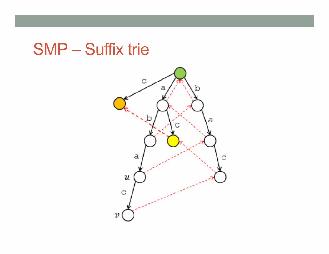
SMP – Suffix trie • Suffix trie of a string T is a rooted tree that stores all the
suffixes (thus all the substrings) • Each node corresponds to some substring of T • Each edge is associated with an alphabet • For each node that corresponds to ax, there is a special
pointer called suffix link that leads to the node corresponding to x
• Surprisingly easy to implement!

SMP – Suffix trie

SMP – Suffix trie • Given the suffix tree for T1 . . . Tn
• Then we append Tn+1 = a to T , creating necessary nodes
• Start at node u corresponding to T1 . . . Tn • Create an a -transition to a new node v
• Take the suffix link at u to go to u′, corresponding to T2 . . . Tn • Create an a -transition to a new node v′ • Create a suffix link from v to v′

SMP – Suffix trie • Repeat the previous process:
• Take the suffix link at the current node • Make a new a-transition there • Create the suffix link from the previous node
• Stop if the node already has an a-transition • Because from this point, all nodes that are reachable via suffix links
already have an a -transition

SMP – Suffix trie • Given the suffix trie for aba, we want to add a new letter c

SMP – Suffix trie

SMP – Suffix trie

SMP – Suffix trie
SMP – Suffix trie

SMP – Suffix trie

SMP – Suffix trie • To find P, start at the root and keep following edges
labeled with P1, P2, etc. • Got stuck? Then P doesn’t exist in T

SMP-Suffix Array

SMP – Suffix Array • Memory usage is O(n) • Has the same computational power as suffix trie • Can be constructed in O(n) time (!)
• But it’s hard to implement

Notes • Always be aware of the null-terminators • Simple hash works so well in many problems • If a problem involves rotations of some string, consider
concatenating it with itself and see if it helps • It is a smart idea to have the implementation of suffix
arrays and KMP in your notebook.