Notes on Excel Forecasting Tools

Data Table, Scenario Manager, Goal Seek, & Solver

2001-2002

Contents Overview ................................................................................................................1

Data Table Scenario Manager Goal Seek Solver

Examples

Data Table ....................................................................................................2 Scenario Manager........................................................................................8 Goal Seek......................................................................................................11 Solver ............................................................................................................12

Appendix

Views of the worksheets in the ForecastingTools.xls workbook

Overview Data Table

Excel’s Data Table is a powerful sensitivity analysis tool that shows how changing certain values in a model’s formulas might affect critical elements of the model. Data tables provide a shortcut for generating multiple views for a model in a single operation as well as a way to view and compare the results of all of the variations together on a single worksheet. There are two varieties of Data Table: one-input and two-input. To run a Data Table, establish the proper Data Table layout and data and then use the commands Data, Table to open the “Table” dialog. Using the prompts in the “Table” dialog, link the Data Table input values to the model and click OK to run.

Scenario Manager

A scenario is a set of values that Excel saves and can substitute on command in a worksheet model. You can create and save different groups of values on a worksheet and then switch to any of these new scenarios to view different model results. For example, if you create a budget worksheet but are uncertain what revenue value to include, you can define different values for the revenue and then switch between the scenarios to perform what-if analyses. To build scenarios, choose Tools, Scenarios to open the “Scenario Manager” dialog. Follow the prompts.

Goal Seek

When you know the result you want from a single formula but not the input value the formula needs to determine the result, use Excel’s Goal Seek. When goal seeking, Excel varies the value in a worksheet cell you specify until the formula that's dependent on that cell returns the result you want.

Solver

Excel’s Solver is a problem-solving tool like Goal Seek; however, the Solver provides a much more powerful and flexible approach. Use Solver to determine the maximum or minimum value of one cell by changing other cells— for example, the maximum profit you can generate by changing advertising expenditures. You specify one or more “changing cells” which must be related through formulas on the worksheet. In addition, you can establish model constraints, and Solver will search for a solution without violating the constraints. Solver adjusts the values in the changing cells you specify to produce the result you want from the formula. Choose Tools, Solver to open the “Solver Parameters” dialog. Solver is an Excel add-in, but is part of Excel. If you don’t find Solver on Excel’s Tools menu, add it with Tools, Add-Ins or return to your Excel software media to add it as an option to your Excel installation.

1

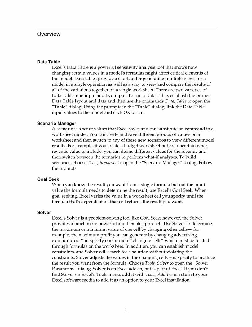
Examples The Data Table The ForecastingTools.xls workbook contains an “Income Statement” worksheet that shows a monthly income statement for Triangle Widgets, Inc. Obtain a copy of this workbook if you want to follow along in Excel.

As you might expect, the imany cells. For example, Rare formulas. One can chanthese formulas. Here are some examples o

What happens to ounits per month ins

If the company sellexpenses if 3000 un

What happens if Tr

1 As the model is currently cocomplex calculations and assfixed expense value for “Advvalue will affect the bottom liyou can’t use this model to anunit sales?”

The Income Statement worksheet.

ncome statement model uses formulas, not static values, for evenue, Total Variable Expenses, and Total Fixed Expenses ge data values in the model and see how those changes affect

f questions you might answer using this model:1 perating income if Triangle Widgets sells 2000, 2500, or 3000 tead of 1000?

s 2000 units how do expenses change? What’s the impact on its are sold? 4000? iangle Widget’s leasing costs go up by 20%? By 25% By 30%?

nstructed there are also some kinds of questions (that involve more umptions) that you can not answer. For example, in this model the ertising” is a static number. While changing the static advertising ne, the model can’t show how a change might affect “Units Sold”. So swer the question “How would an increase in advertising affect

2

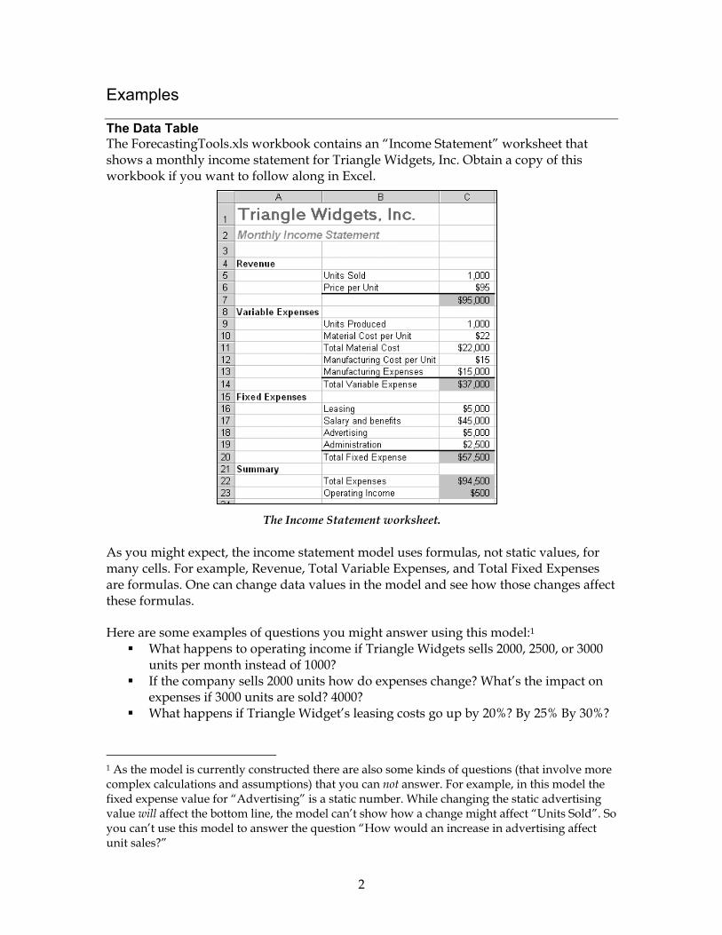
What happens if manufacturing costs go down by an eighth? By a quarter? By a third?

Many questions of this kind can be quickly answered for a wide range of possible values by using one of Excel’s powerful forecasting tools, the Data Table. Some of the advantages of using a Data Table for this kind of task instead of just changing values in the model itself are:

You can include any number of substitute (changing) values in the Data Table. For example, with a Data Table it’s easy how a wide range of production level values affects operating income instead of viewing the effect of each possible production level in the model viewed one at a time.

The results are visible in a conveniently small matrix.

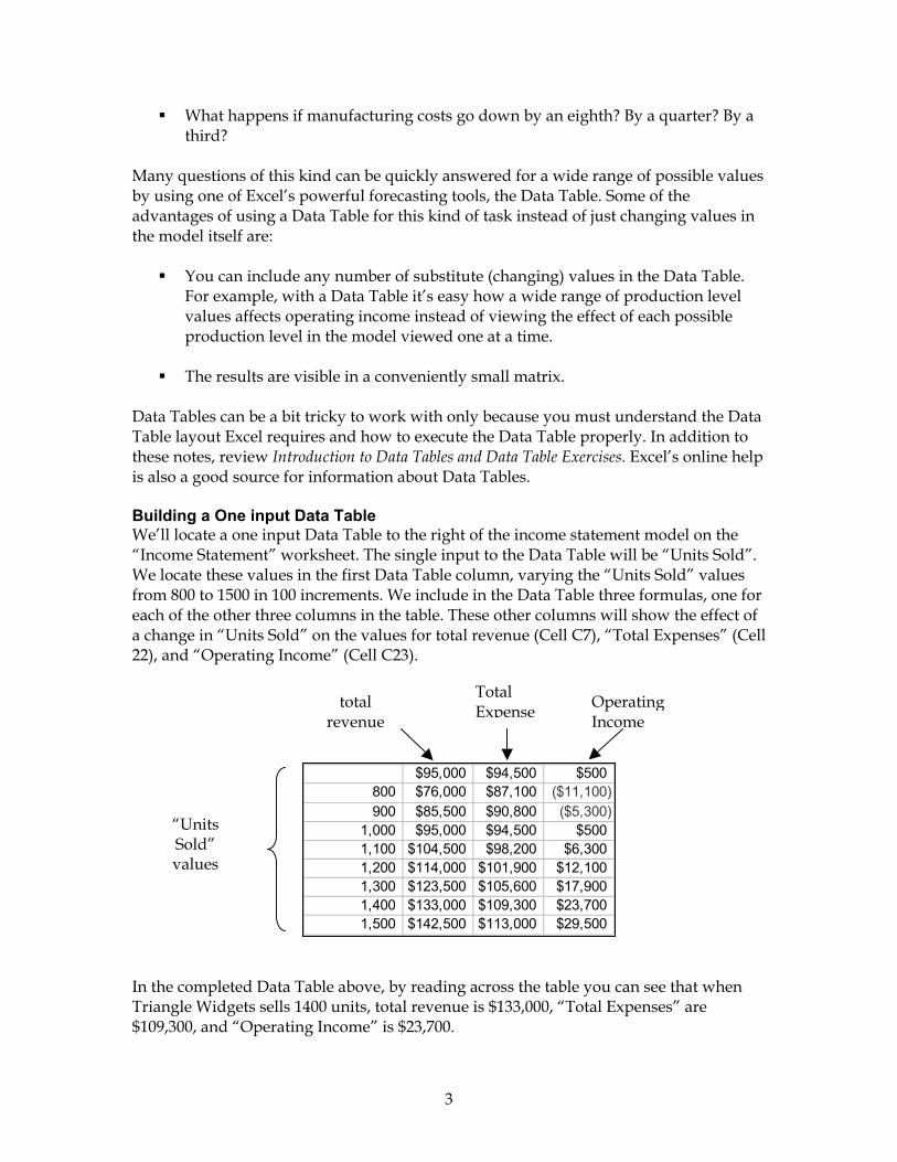
Data Tables can be a bit tricky to work with only because you must understand the Data Table layout Excel requires and how to execute the Data Table properly. In addition to these notes, review Introduction to Data Tables and Data Table Exercises. Excel’s online help is also a good source for information about Data Tables. Building a One input Data Table We’ll locate a one input Data Table to the right of the income statement model on the “Income Statement” worksheet. The single input to the Data Table will be “Units Sold”. We locate these values in the first Data Table column, varying the “Units Sold” values from 800 to 1500 in 100 increments. We include in the Data Table three formulas, one for each of the other three columns in the table. These other columns will show the effect of a change in “Units Sold” on the values for total revenue (Cell C7), “Total Expenses” (Cell 22), and “Operating Income” (Cell C23).

r

“Units Sold” values

In the completed Data TableTriangle Widgets sells 1400 $109,300, and “Operating In

total evenue

$95,000800 $76,000900 $85,500

1,000 $95,0001,100 $104,5001,200 $114,0001,300 $123,5001,400 $133,0001,500 $142,500

above, by readingunits, total revenuecome” is $23,700.

3

Total Expense

$94,500 $$87,100 ($11,$90,800 ($5,$94,500 $$98,200 $6,

$101,900 $12,$105,600 $17,$109,300 $23,$113,000 $29,

across the table is $133,000, “To

Operating Income

500100)300)500300100900700500

you can see that when tal Expenses” are

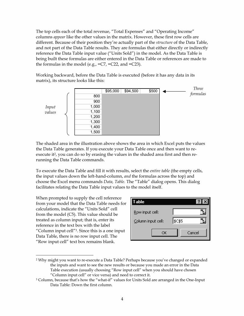
The top cells each of the total revenue, “Total Expenses” and “Operating Income” columns appear like the other values in the matrix. However, these first row cells are different. Because of their position they’re actually part of the structure of the Data Table, and not part of the Data Table results. They are formulas that either directly or indirectly reference the Data Table input value (“Units Sold”) in the model. As the Data Table is being built these formulas are either entered in the Data Table or references are made to the formulas in the model (e.g., =C7, =C22, and =C23). Working backward, before the Data Table is executed (before it has any data in its matrix), its structure looks like this:

$95,000 $94,500 $500800 900

1,000 1,100 1,200 1,300 1,400 1,500

Input values

Three formulas

The shaded area in the illustration above shows the area in which Excel puts the values the Data Table generates. If you execute your Data Table once and then want to re-execute it2, you can do so by erasing the values in the shaded area first and then re-running the Data Table commands. To execute the Data Table and fill it with results, select the entire table (the empty cells, the input values down the left-hand-column, and the formulas across the top) and choose the Excel menu commands Data, Table. The “Table” dialog opens. This dialog facilitates relating the Data Table input values to the model itself. When prompted to supply the cell reference from your model that the Data Table needs for calculations, indicate the “Units Sold” cell from the model (C5). This value should be treated as column input; that is, enter its reference in the text box with the label “Column input cell”3. Since this is a one input Data Table, there is no row input cell. The “Row input cell” text box remains blank.

2 Why might you want to re-execute a Data Table? Perhaps because you’ve changed or expanded

the inputs and want to see the new results or because you made an error in the Data Table execution (usually choosing “Row input cell” when you should have chosen “Column input cell” or vice versa) and need to correct it.

3 Column, because that’s how the “what-if” values for Units Sold are arranged in the One-Input Data Table: Down the first column.

4

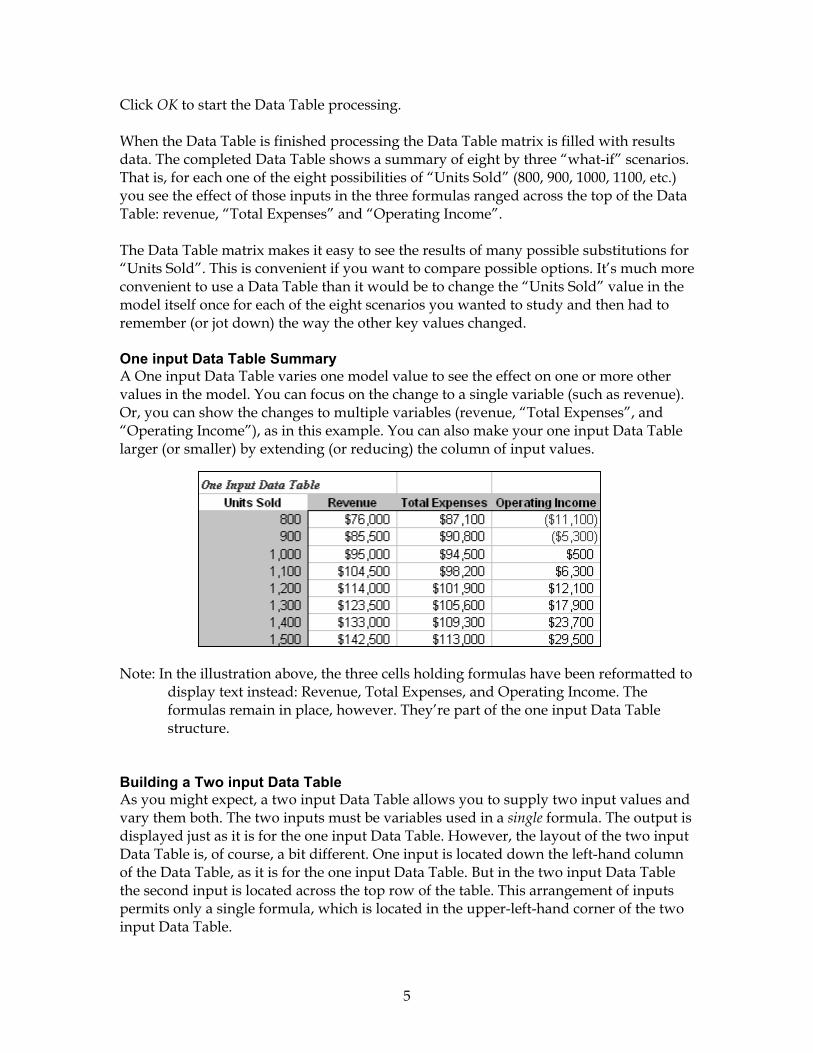
Click OK to start the Data Table processing. When the Data Table is finished processing the Data Table matrix is filled with results data. The completed Data Table shows a summary of eight by three “what-if” scenarios. That is, for each one of the eight possibilities of “Units Sold” (800, 900, 1000, 1100, etc.) you see the effect of those inputs in the three formulas ranged across the top of the Data Table: revenue, “Total Expenses” and “Operating Income”. The Data Table matrix makes it easy to see the results of many possible substitutions for “Units Sold”. This is convenient if you want to compare possible options. It’s much more convenient to use a Data Table than it would be to change the “Units Sold” value in the model itself once for each of the eight scenarios you wanted to study and then had to remember (or jot down) the way the other key values changed. One input Data Table Summary A One input Data Table varies one model value to see the effect on one or more other values in the model. You can focus on the change to a single variable (such as revenue). Or, you can show the changes to multiple variables (revenue, “Total Expenses”, and “Operating Income”), as in this example. You can also make your one input Data Table larger (or smaller) by extending (or reducing) the column of input values.

Note: In the illustration above, the three cells holding formulas have been reformatted to

display text instead: Revenue, Total Expenses, and Operating Income. The formulas remain in place, however. They’re part of the one input Data Table structure.

Building a Two input Data Table As you might expect, a two input Data Table allows you to supply two input values and vary them both. The two inputs must be variables used in a single formula. The output is displayed just as it is for the one input Data Table. However, the layout of the two input Data Table is, of course, a bit different. One input is located down the left-hand column of the Data Table, as it is for the one input Data Table. But in the two input Data Table the second input is located across the top row of the table. This arrangement of inputs permits only a single formula, which is located in the upper-left-hand corner of the two input Data Table.

5

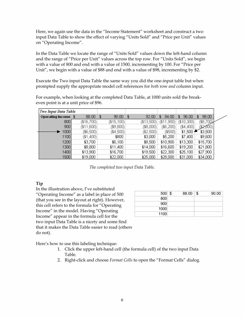
Here, we again use the data in the “Income Statement” worksheet and construct a two input Data Table to show the effect of varying “Units Sold” and “Price per Unit” values on “Operating Income”. In the Data Table we locate the range of “Units Sold” values down the left-hand column and the range of “Price per Unit” values across the top row. For “Units Sold”, we begin with a value of 800 and end with a value of 1500, incrementing by 100. For “Price per Unit”, we begin with a value of $88 and end with a value of $98, incrementing by $2. Execute the Two input Data Table the same way you did the one-input table but when prompted supply the appropriate model cell references for both row and column input. For example, when looking at the completed Data Table, at 1000 units sold the break-even point is at a unit price of $96.

The completed two input Data Table.

Tip In the illustration above, I’ve substituted “Operating Income” as a label in place of 500 (that you see in the layout at right). However, this cell refers to the formula for “Operating Income” in the model. Having “Operating Income” appear in the formula cell for the

500 88.00$ 90.00$ 800900

10001100

two input Data Table is a nicety and some find that it makes the Data Table easier to read (others do not). Here’s how to use this labeling technique:

1. Click the upper left-hand cell (the formula cell) of the two input Data Table.

2. Right-click and choose Format Cells to open the “Format Cells” dialog.

6

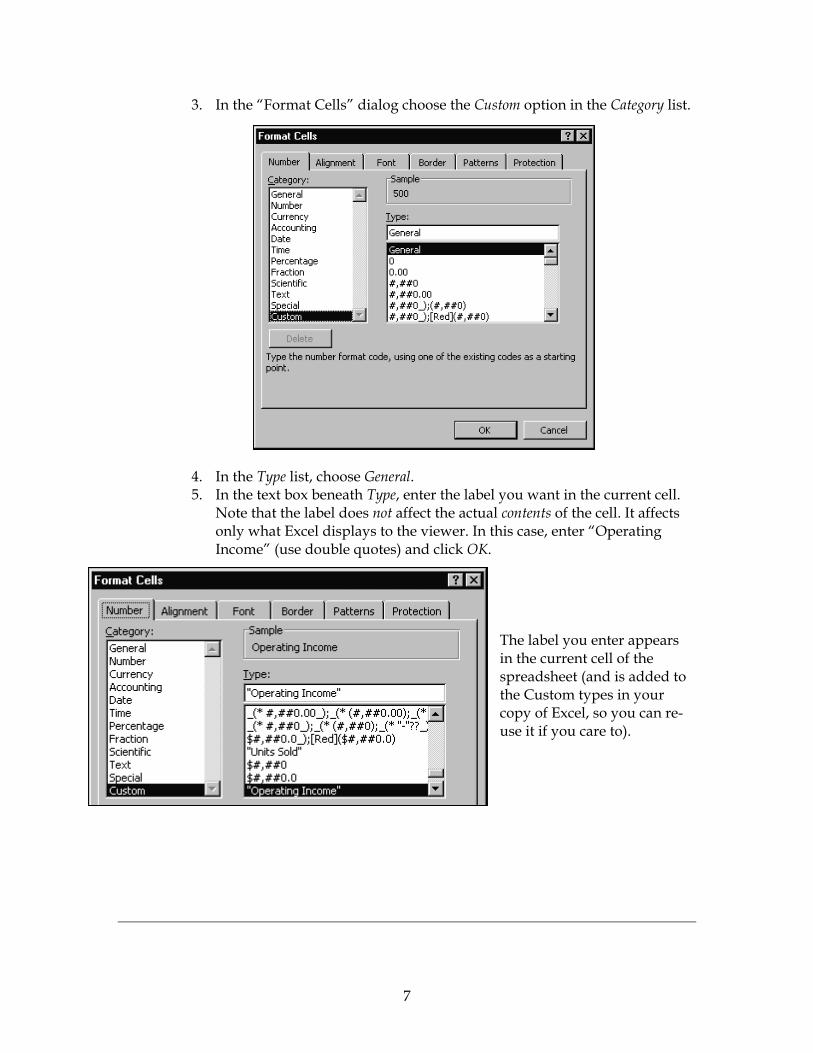
3. In the “Format Cells” dialog choose the Custom option in the Category list.

4. In the Type list, choose General. 5. In the text box beneath Type, enter the label you want in the current cell.

Note that the label does not affect the actual contents of the cell. It affects only what Excel displays to the viewer. In this case, enter “Operating Income” (use double quotes) and click OK.

The label you enter appears in the current cell of the spreadsheet (and is added to the Custom types in your copy of Excel, so you can re-use it if you care to).

7

Scenario Manager For an example of the Scenario Manager we again return to the “Income Statement” worksheet in the ForecastingTools.xls workbook. Above, we generated two kinds of Data Tables to summarize how a change in one or two values affect other values in the model. Here, we do something similar. However, instead of showing the changed values in a tabular format we show a number of possible variations individually as different worksheet scenarios. This method has the advantage of allowing the viewer to see the changes within the worksheet itself and is often useful if you have a small number of scenarios you want to work with or present. We use Excel’s Scenario Manager to create three scenarios: Low Cost, Competitive, and High Cost. For each one of the three scenarios, we changes to these three values in the model: “Units Sold”, “Price per Unit”, and “Material Cost per Unit” as indicated in the table below:

Low Cost Competitive High Cost Changing Cells: Units_Sold 1,400 1,300 1,200 Price_per_Unit $80 $90 $100 Material_Cost_per_Unit $22 $24 $26

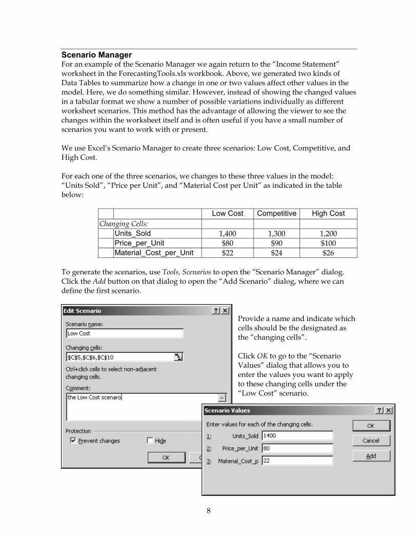
To generate the scenarios, use Tools, Scenarios to open the “Scenario Manager” dialog. Click the Add button on that dialog to open the “Add Scenario” dialog, where we can define the first scenario.

Provide a name and indicate which cells should be the designated as the “changing cells”. Click OK to go to the “Scenario Values” dialog that allows you to enter the values you want to apply to these changing cells under the “Low Cost” scenario.

8

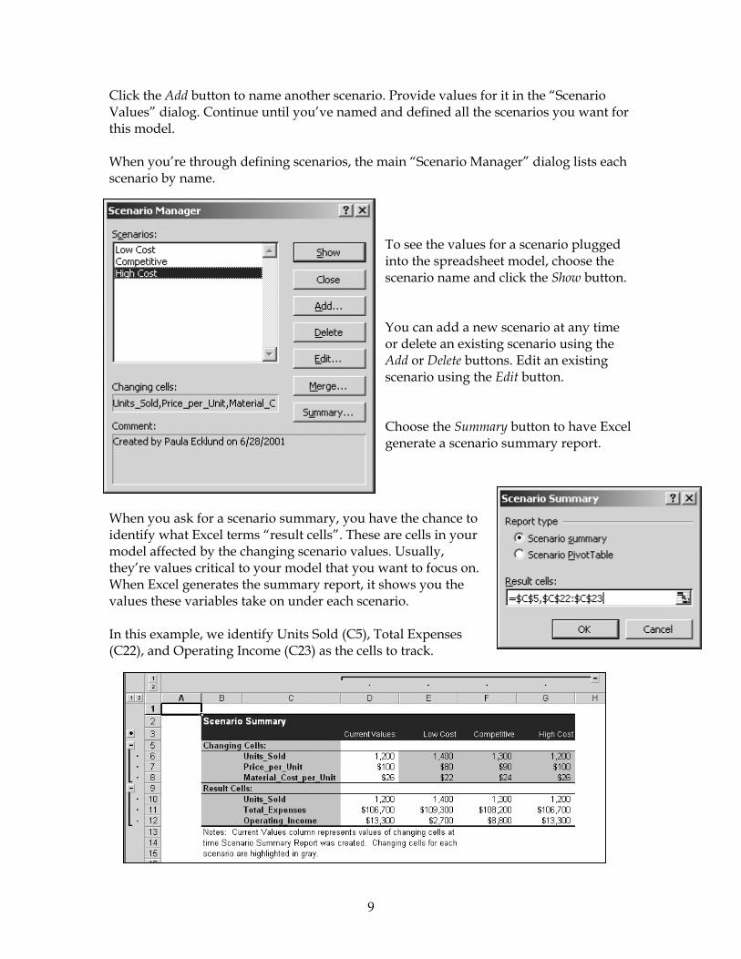
Click the Add button to name another scenario. Provide values for it in the “Scenario Values” dialog. Continue until you’ve named and defined all the scenarios you want for this model. When you’re through defining scenarios, the main “Scenario Manager” dialog lists each scenario by name.

To see the values for a scenario plugged into the spreadsheet model, choose the scenario name and click the Show button. You can add a new scenario at any time or delete an existing scenario using the Add or Delete buttons. Edit an existing scenario using the Edit button. Choose the Summary button to have Excel generate a scenario summary report.

When you ask for a scenario summary, you have the chance to identify what Excel terms “result cells”. These are cells in your model affected by the changing scenario values. Usually, they’re values critical to your model that you want to focus on. When Excel generates the summary report, it shows you the values these variables take on under each scenario. In this example, we identify Units Sold (C5), Total Expenses (C22), and Operating Income (C23) as the cells to track.

9

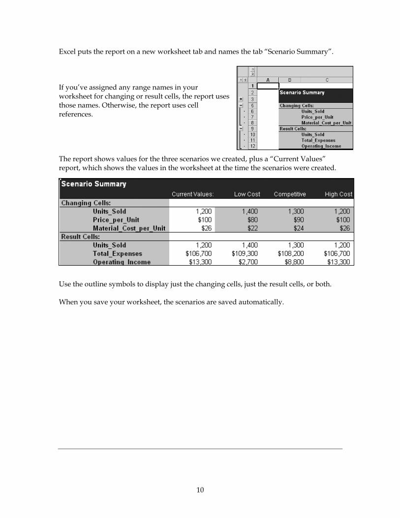
Excel puts the report on a new worksheet tab and names the tab “Scenario Summary”. If you’ve assigned any range names in your worksheet for changing or result cells, the report uses those names. Otherwise, the report uses cell references. The report shows values for the three scenarios we created, plus a “Current Values” report, which shows the values in the worksheet at the time the scenarios were created.

Use the outline symbols to display just the changing cells, just the result cells, or both. When you save your worksheet, the scenarios are saved automatically.

10

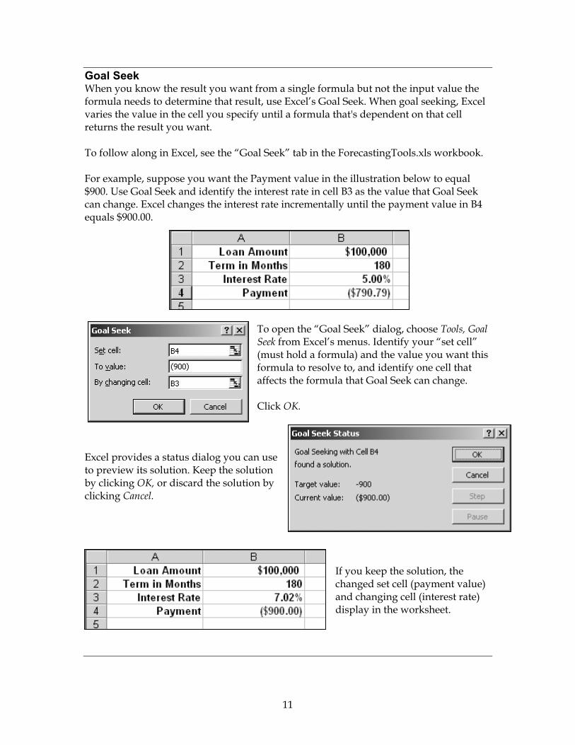
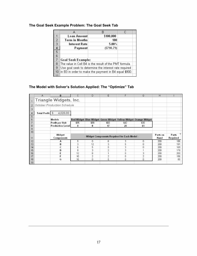
Goal Seek When you know the result you want from a single formula but not the input value the formula needs to determine that result, use Excel’s Goal Seek. When goal seeking, Excel varies the value in the cell you specify until a formula that's dependent on that cell returns the result you want. To follow along in Excel, see the “Goal Seek” tab in the ForecastingTools.xls workbook. For example, suppose you want the Payment value in the illustration below to equal $900. Use Goal Seek and identify the interest rate in cell B3 as the value that Goal Seek can change. Excel changes the interest rate incrementally until the payment value in B4 equals $900.00.

To open the “Goal Seek” dialog, choose Tools, Goal Seek from Excel’s menus. Identify your “set cell” (must hold a formula) and the value you want this formula to resolve to, and identify one cell that affects the formula that Goal Seek can change. Click OK.

Excel provides a status dialog you can use to preview its solution. Keep the solution by clicking OK, or discard the solution by clicking Cancel.

If you keep the solution, the changed set cell (payment value) and changing cell (interest rate) display in the worksheet.

11

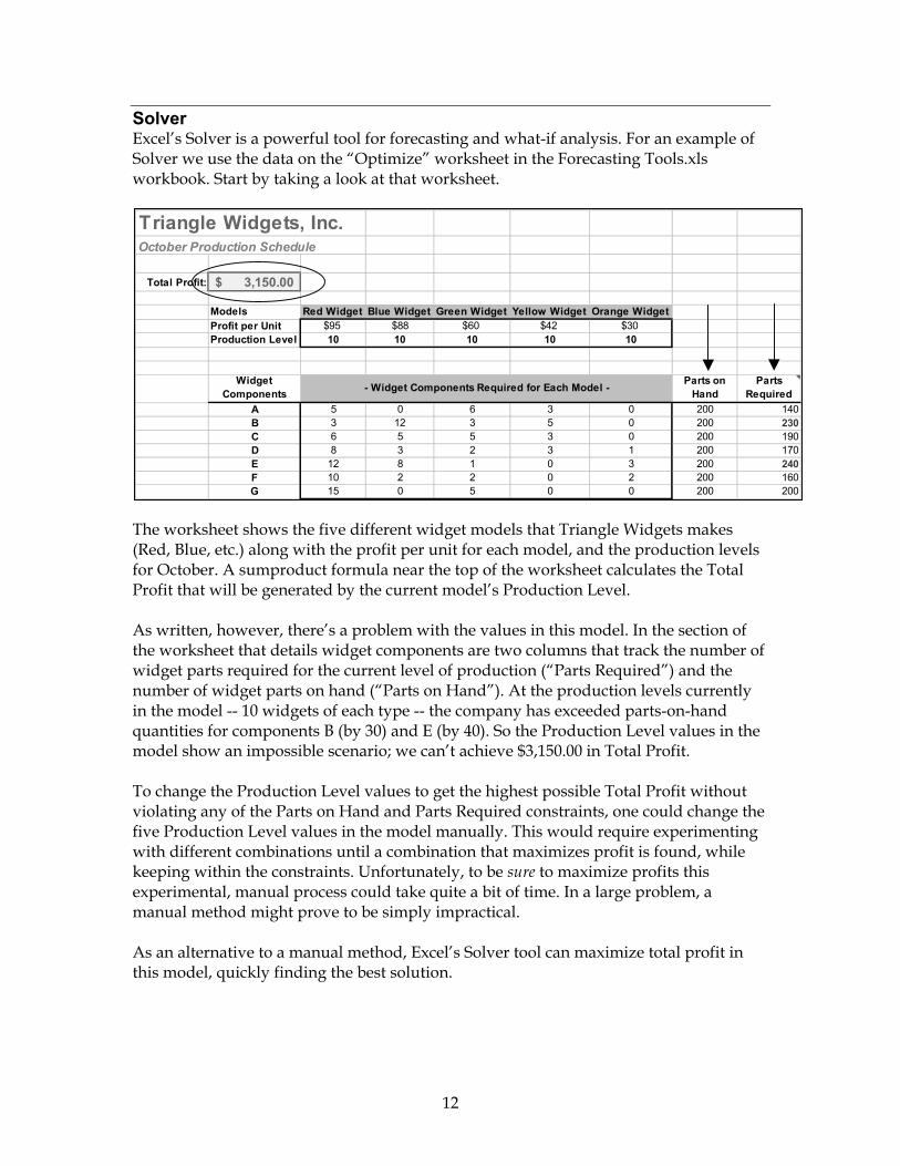
Solver Excel’s Solver is a powerful tool for forecasting and what-if analysis. For an example of Solver we use the data on the “Optimize” worksheet in the Forecasting Tools.xls workbook. Start by taking a look at that worksheet.

Triangle Widgets, Inc.October Production Schedule

Total Profit: 3,150.00$

Models Red Widget Blue Widget Green Widget Yellow Widget Orange WidgetProfit per Unit $95 $88 $60 $42 $30Production Level 10 10 10 10 10

Widget Components

Parts on Hand

Parts Required

A 5 0 6 3 0 200B 3 12 3 5 0 200 230C 6 5 5 3 0 200D 8 3 2 3 1 200E 12 8 1 0 3 200 240F 10 2 2 0 2 200 160G 15 0 5 0 0 200 200

- Widget Components Required for Each Model -

140

190170

The worksheet shows the five different widget models that Triangle Widgets makes (Red, Blue, etc.) along with the profit per unit for each model, and the production levels for October. A sumproduct formula near the top of the worksheet calculates the Total Profit that will be generated by the current model’s Production Level. As written, however, there’s a problem with the values in this model. In the section of the worksheet that details widget components are two columns that track the number of widget parts required for the current level of production (“Parts Required”) and the number of widget parts on hand (“Parts on Hand”). At the production levels currently in the model -- 10 widgets of each type -- the company has exceeded parts-on-hand quantities for components B (by 30) and E (by 40). So the Production Level values in the model show an impossible scenario; we can’t achieve $3,150.00 in Total Profit. To change the Production Level values to get the highest possible Total Profit without violating any of the Parts on Hand and Parts Required constraints, one could change the five Production Level values in the model manually. This would require experimenting with different combinations until a combination that maximizes profit is found, while keeping within the constraints. Unfortunately, to be sure to maximize profits this experimental, manual process could take quite a bit of time. In a large problem, a manual method might prove to be simply impractical. As an alternative to a manual method, Excel’s Solver tool can maximize total profit in this model, quickly finding the best solution.

12

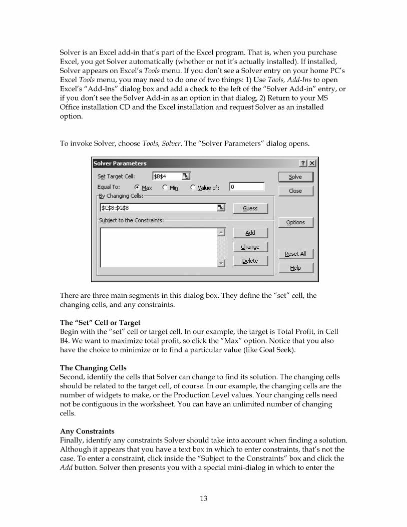
Solver is an Excel add-in that’s part of the Excel program. That is, when you purchase Excel, you get Solver automatically (whether or not it’s actually installed). If installed, Solver appears on Excel’s Tools menu. If you don’t see a Solver entry on your home PC’s Excel Tools menu, you may need to do one of two things: 1) Use Tools, Add-Ins to open Excel’s “Add-Ins” dialog box and add a check to the left of the “Solver Add-in” entry, or if you don’t see the Solver Add-in as an option in that dialog, 2) Return to your MS Office installation CD and the Excel installation and request Solver as an installed option. To invoke Solver, choose Tools, Solver. The “Solver Parameters” dialog opens.

There are three main segments in this dialog box. They define the “set” cell, the changing cells, and any constraints. The “Set” Cell or Target Begin with the “set” cell or target cell. In our example, the target is Total Profit, in Cell B4. We want to maximize total profit, so click the “Max” option. Notice that you also have the choice to minimize or to find a particular value (like Goal Seek). The Changing Cells Second, identify the cells that Solver can change to find its solution. The changing cells should be related to the target cell, of course. In our example, the changing cells are the number of widgets to make, or the Production Level values. Your changing cells need not be contiguous in the worksheet. You can have an unlimited number of changing cells. Any Constraints Finally, identify any constraints Solver should take into account when finding a solution. Although it appears that you have a text box in which to enter constraints, that’s not the case. To enter a constraint, click inside the “Subject to the Constraints” box and click the Add button. Solver then presents you with a special mini-dialog in which to enter the

13

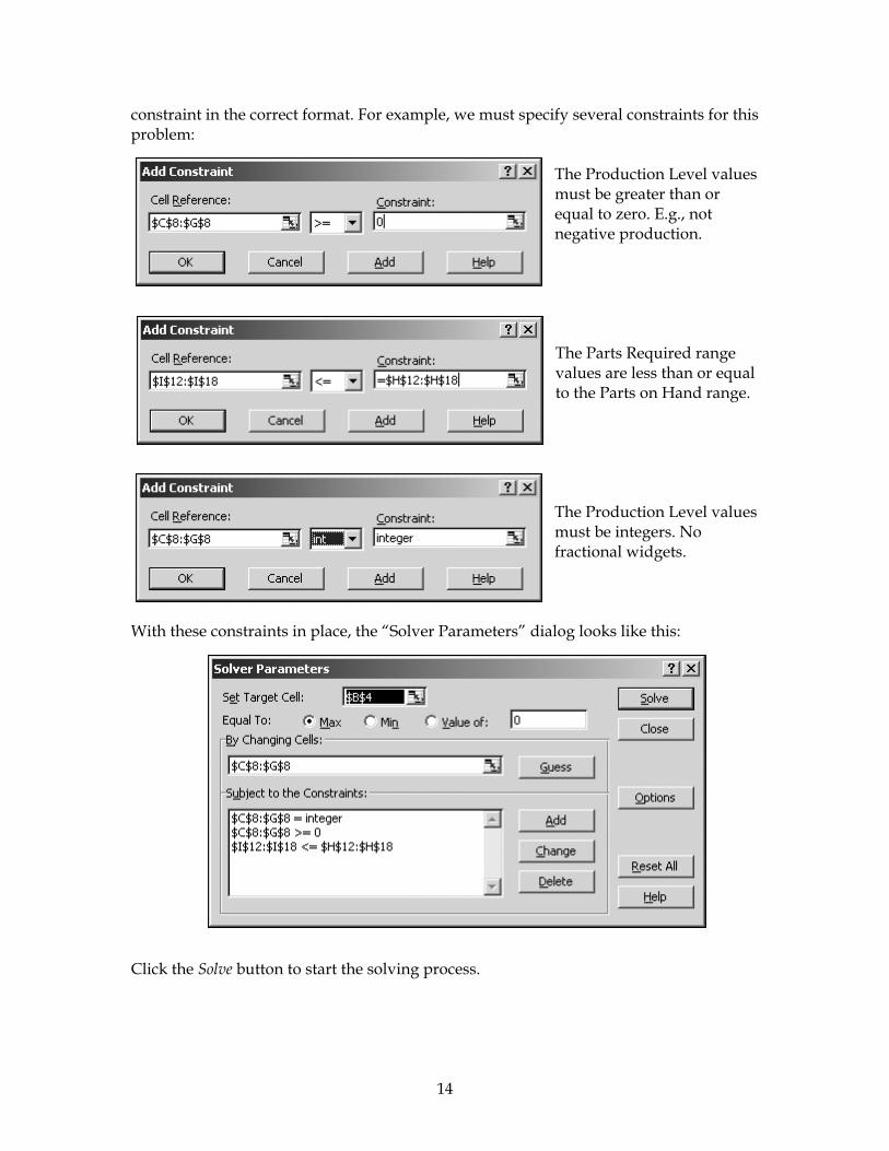
constraint in the correct format. For example, we must specify several constraints for this problem:

The Production Level values must be greater than or equal to zero. E.g., not negative production. The Parts Required range values are less than or equal to the Parts on Hand range. The Production Level values must be integers. No fractional widgets.

With these constraints in place, the “Solver Parameters” dialog looks like this: Click the Solve button to start the solving process.

14

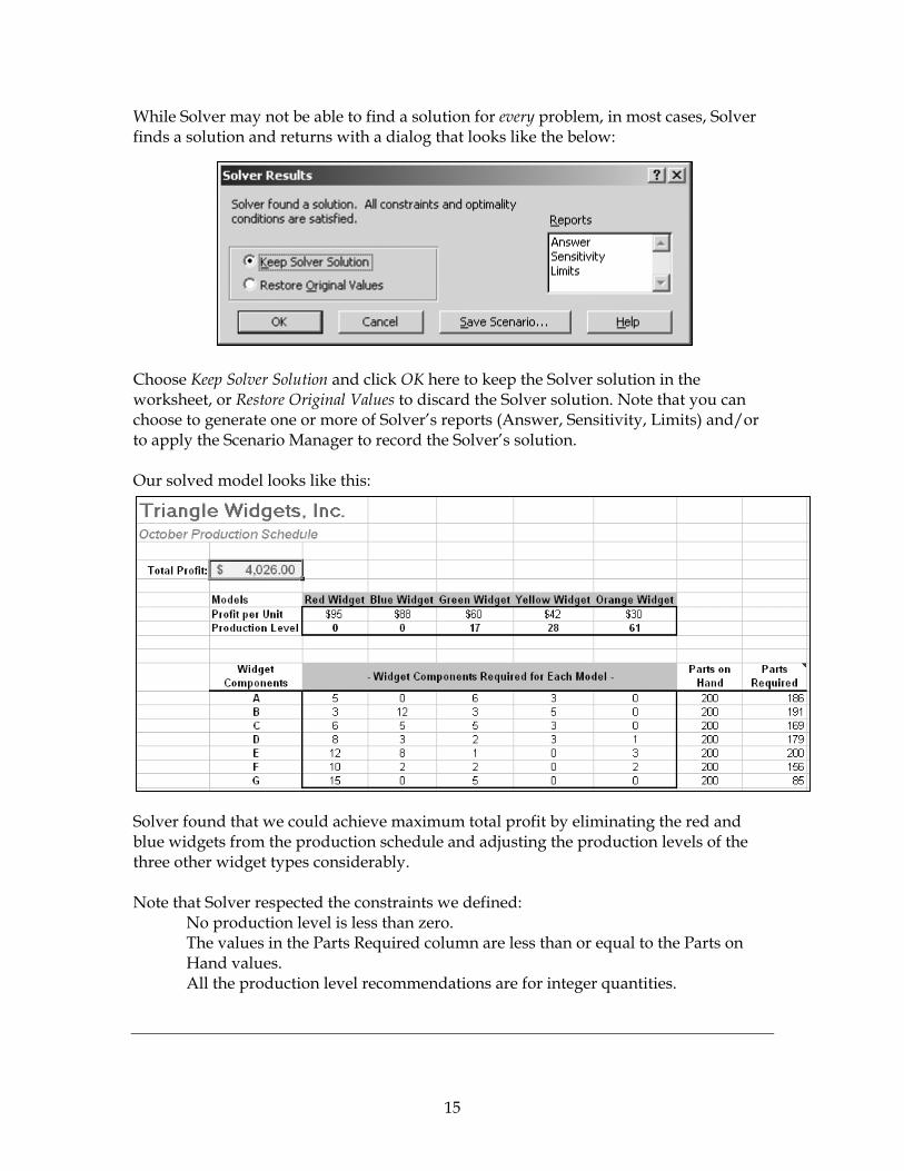
While Solver may not be able to find a solution for every problem, in most cases, Solver finds a solution and returns with a dialog that looks like the below: Choose Keep Solver Solution and click OK here to keep the Solver solution in the worksheet, or Restore Original Values to discard the Solver solution. Note that you can choose to generate one or more of Solver’s reports (Answer, Sensitivity, Limits) and/or to apply the Scenario Manager to record the Solver’s solution. Our solved model looks like this:

Solver found that we could achieve maximum total profit by eliminating the red and blue widgets from the production schedule and adjusting the production levels of the three other widget types considerably. Note that Solver respected the constraints we defined:

No production level is less than zero. The values in the Parts Required column are less than or equal to the Parts on Hand values. All the production level recommendations are for integer quantities.

15

16

A ppendix Views of the worksheets in the accompanying ForecastingTools.xls workbook.

Data Tables: the Income Statement Tab

The Scenario Report: The Scenario Summary Tab

The Goal Seek Example Problem: The Goal Seek Tab The Model with Solver’s Solution Applied: The “Optimize” Tab

17