6.1 Lab 6 (Topic 8)

BIOL 933 Lab 6 Fall 2017

Data Transformation

· Transformations in R · General overview · Log transformation · Power transformation

· The pitfalls of interpreting interactions in transformed data Transformations in R "Data transformation" is a fancy term for changing the values of observations through some mathematical operation. Such transformations are simple in R and assume a form that should be very familiar to you by now:

data_dat$trans_Y <- sqrt(data_dat$Y) The above code tells R to create a new variable (or column in the data_dat dataset) named "trans_Y" that is equal to the square root of the original response variable Y. We’ve seen this basic trick before (e.g. appending residual and predicted values to a dataframe). While R can handle just about any mathematical operation you can throw at it, the syntax for such things is not always intuitive. So here are some other examples that we could have used in the above sample code:

data_dat$trans_Y <- (data_dat$Y)^3 Raises Y to the power of 3 data_dat$trans_Y <- (data_dat$Y)^(1/9) Takes the ninth root of Y data_dat$trans_Y <- log(data_dat$Y) Takes the natural logarithm (ln) of Y data_dat$trans_Y <- log10(data_dat$Y) Takes the base-10 logarithm of Y data_dat$trans_Y <- exp(data_dat$Y) Raises the constant e to the power of Y data_dat$trans_Y <- abs(data_dat$Y) Finds the absolute value of Y data_dat$trans_Y <- sin(data_dat$Y) Calculates the sine of Y data_dat$trans_Y <- asin(data_dat$Y) Calculates the inverse sine (arcsine) of Y Etc…

You can create as many derived variables as you wish; and you can calculate new variables that refer to other derived variables, e.g. data_dat$trans1_Y <- sqrt(data_dat$Y) data_dat$trans2_Y <- sin(data_dat$trans1_Y)

But now for some real examples.

6.2 Lab 6 (Topic 8)

Log Transformation Example 1 From Little and Hills [Lab6ex1.R] In this experiment, the effect of vitamin supplements on weight gain is being investigated in three animal species (mice, chickens, and sheep). The experiment is designed as an RCBD with one replication (i.e. animal) per block*treatment combination. The six treatment levels are MC (mouse control), MV (mouse + vitamin), CC (chicken control), CV (chicken + vitamin), SC (sheep control), and SV (sheep + vitamin). The response variable is the weight of the animal at the end of the experiment.

trtmt block weightMC I 0.18MC II 0.3MC III 0.28... ... ...SV II 153SV III 148SV IV 176

#read in, re-classify, and inspect the data vit_dat<-as.data.frame(vit_dat) vit_dat$block<-as.factor(vit_dat$block) vit_dat$trtmt<-as.factor(vit_dat$trtmt) str(vit_dat, give.attr = F) #The ANOVA vit_mod<-lm(weight ~ trtmt + block, vit_dat) anova(vit_mod) #Need to assign contrast coefficients #Notice from str() that R orders the Trtmt levels this way: CC,CV,MC,etc... # Our desired contrasts: # Contrast ‘Mam vs. Bird’ 2,2,-1,-1,-1,-1 # Contrast ‘Mouse vs. Sheep' 0,0,1,1,-1,-1 # Contrast ‘Vit’ 1,-1,1,-1,1,-1 # Contrast ‘MamBird*Vit’ 2,-2,-1,1,-1,1 # Contrast ‘MouShe*Vit’ 0,0,1,-1,-1,1 contrastmatrix<-cbind(c(2,2,-1,-1,-1,-1),c(0,0,1,1,-1,-1),c(1,-1,1,-1,1,-1),c(2,-2,-1,1,-1,1),c(0,0,1,-1,-1,1)) contrasts(vit_dat$trtmt)<-contrastmatrix log_contrast_mod<-aov(weight ~ trtmt + block, vit_dat) summary(log_contrast_mod, split = list(trtmt = list("MvsB" = 1, "MvsS" = 2, "Vit" = 3, "MB*Vit" = 4, "MS*Vit" = 5))) #TESTING ASSUMPTIONS #Generate residual and predicted values vit_dat$resids <- residuals(vit_mod)

6.3 Lab 6 (Topic 8)

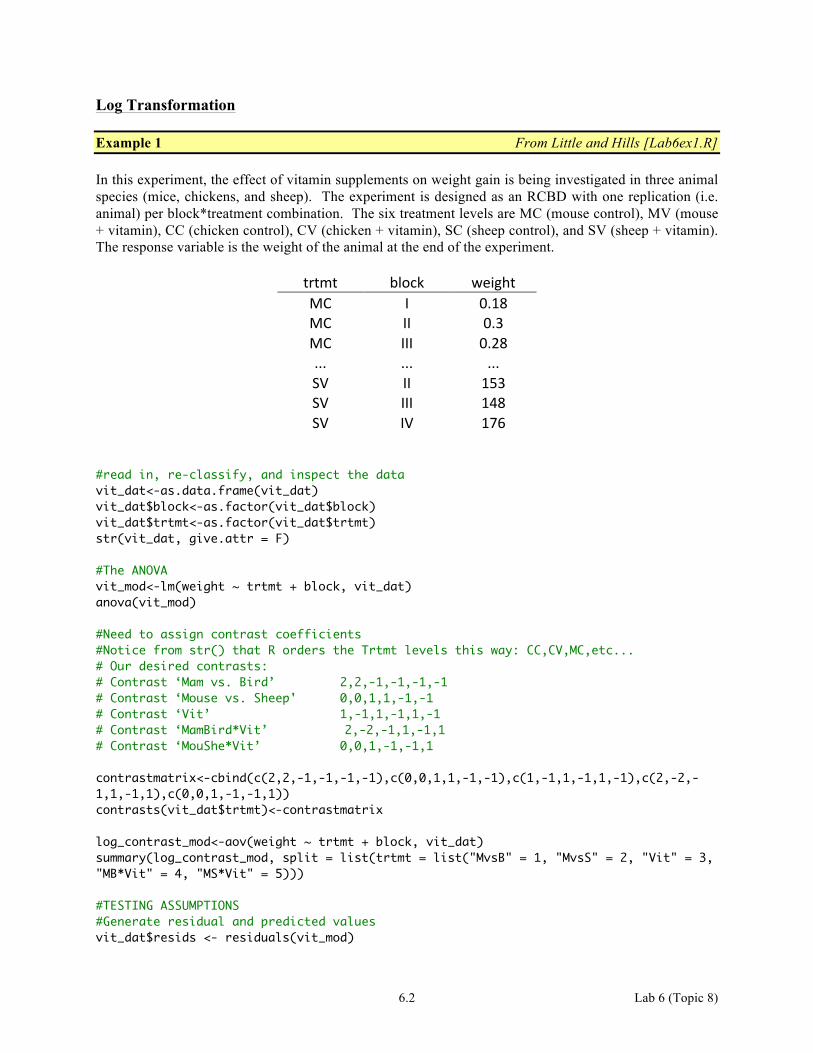
vit_dat$preds <- predict(vit_mod) vit_dat$sq_preds <- vit_dat$preds^2 #Look at a plot of residual vs. predicted values plot(resids ~ preds, data = vit_dat, xlab = "Predicted Values", ylab = "Residuals") #Perform a Shapiro-Wilk test for normality of residuals shapiro.test(vit_dat$resids) #Perform Levene's Test for homogenity of variances #install.packages("car") library(car) leveneTest(weight ~ trtmt, data = vit_dat) #Perform a Tukey 1-df Test for Non-additivity log_1df_mod<-lm(weight ~ trtmt + block + sq_preds, vit_dat) anova(log_1df_mod) The ANOVA Df Sum Sq Mean Sq F value Pr(>F) trtmt 5 108714 21743 174.433 9.77e-13 *** trtmt: MvsB 1 25780 25780 206.821 3.51e-10 *** trtmt: MvsS 1 82541 82541 662.193 7.97e-14 *** trtmt: Vit 1 142 142 1.140 0.3025 trtmt: MB*Vit 1 57 57 0.459 0.5084 trtmt: MS*Vit 1 193 193 1.550 0.2322 block 3 984 328 2.631 0.0881 . Residuals 15 1870 125 Test for normality of residuals Shapiro-Wilk normality test data: vit_dat$resids W = 0.9536, p-value = 0.3236 NS Test for homogeneity of variance among treatments Levene's Test for Homogeneity of Variance (center = median) Df F value Pr(>F) group 5 3.3749 0.0252 *

Levene's Test is significant. The res vs. pred plot will illustrate this.

6.4 Lab 6 (Topic 8)

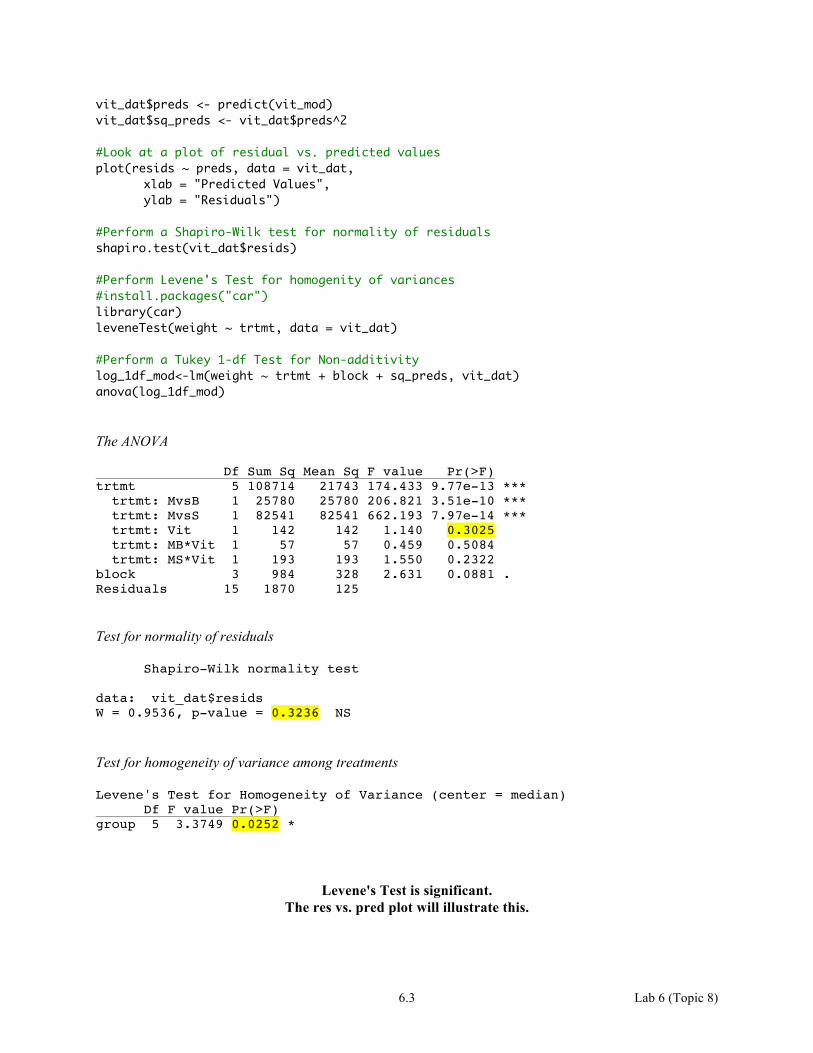
Test for nonadditivity Df Sum Sq Mean Sq F value Pr(>F) trtmt 5 108714 21742.7 6506.417 < 2.2e-16 *** block 3 984 328.0 98.153 1.222e-09 *** sq_preds 1 1823 1822.9 545.507 1.301e-12 *** Residuals 14 47 3.3

DANGER DANGER WILL ROBINSON!!! SIGNIFICANT NON-ADDITIVE EFFECT! MUST TRANSFORM DATA!

Status: We violated our assumption of additivity, and Levene's Test for Treatment is significant.

What to do? First thing's first: Read your tea leaves…

It's smiling at you.

Now take a look at the means, standard deviations, and variances: Trtmt Mean Std Dev Variance MC 0.3000000 0.1070825 0.0114667 MV 0.4000000 0.0588784 0.0034667 CC 2.4000000 0.5887841 0.3466667 CV 2.9000000 0.4618802 0.2133333 SC 137.0000000 23.3666429 546.0000000 SV 151.0000000 20.1163284 404.6666667

Between mice and sheep, the mean increases by a factor of about 400, the standard deviation increases by a factor of about 270, and the variance increases by a factor of about 73,000!

6.5 Lab 6 (Topic 8)

The situation we face is this:

1. Significant Tukey Test for Nonadditivity 2. The standard deviation scales with the mean 3. The Res vs. Pred plot is smiling tauntingly at you

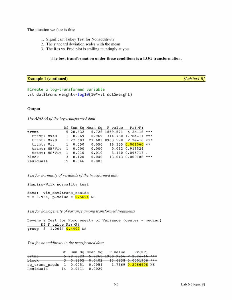
The best transformation under these conditions is a LOG transformation.

Example 1 (continued) [Lab5ex1.R] #Create a log-transformed variable vit_dat$trans_weight<-log10(10*vit_dat$weight) Output The ANOVA of the log-transformed data Df Sum Sq Mean Sq F value Pr(>F) trtmt 5 28.632 5.726 1859.571 < 2e-16 *** trtmt: MvsB 1 0.969 0.969 314.750 1.78e-11 *** trtmt: MvsS 1 27.603 27.603 8963.598 < 2e-16 *** trtmt: Vit 1 0.050 0.050 16.355 0.001060 ** trtmt: MB*Vit 1 0.000 0.000 0.012 0.913524 trtmt: MS*Vit 1 0.010 0.010 3.140 0.096717 . block 3 0.120 0.040 13.043 0.000186 *** Residuals 15 0.046 0.003 Test for normality of residuals of the transformed data Shapiro-Wilk normality test data: vit_dat$trans_resids W = 0.966, p-value = 0.5694 NS Test for homogeneity of variance among transformed treatments Levene's Test for Homogeneity of Variance (center = median) Df F value Pr(>F) group 5 1.0094 0.4407 NS Test for nonadditivity in the transformed data Df Sum Sq Mean Sq F value Pr(>F) trtmt 5 28.6323 5.7265 1950.9256 < 2.2e-16 *** block 3 0.1205 0.0402 13.6838 0.0001906 *** sq_trans_preds 1 0.0051 0.0051 1.7369 0.2086908 NS Residuals 14 0.0411 0.0029

6.6 Lab 6 (Topic 8)

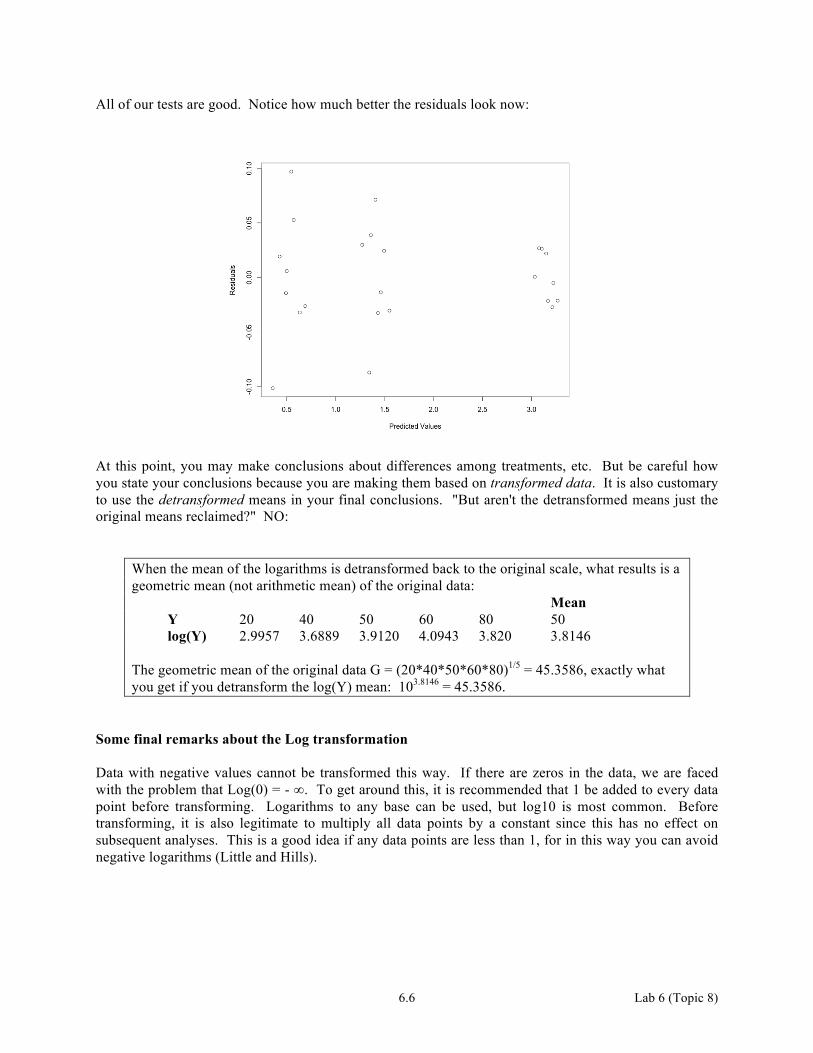
All of our tests are good. Notice how much better the residuals look now:

At this point, you may make conclusions about differences among treatments, etc. But be careful how you state your conclusions because you are making them based on transformed data. It is also customary to use the detransformed means in your final conclusions. "But aren't the detransformed means just the original means reclaimed?" NO:

When the mean of the logarithms is detransformed back to the original scale, what results is a geometric mean (not arithmetic mean) of the original data: Mean Y 20 40 50 60 80 50 log(Y) 2.9957 3.6889 3.9120 4.0943 3.820 3.8146 The geometric mean of the original data G = (20*40*50*60*80)1/5 = 45.3586, exactly what you get if you detransform the log(Y) mean: 103.8146 = 45.3586.

Some final remarks about the Log transformation Data with negative values cannot be transformed this way. If there are zeros in the data, we are faced with the problem that Log(0) = - ∞. To get around this, it is recommended that 1 be added to every data point before transforming. Logarithms to any base can be used, but log10 is most common. Before transforming, it is also legitimate to multiply all data points by a constant since this has no effect on subsequent analyses. This is a good idea if any data points are less than 1, for in this way you can avoid negative logarithms (Little and Hills).

6.7 Lab 6 (Topic 8)

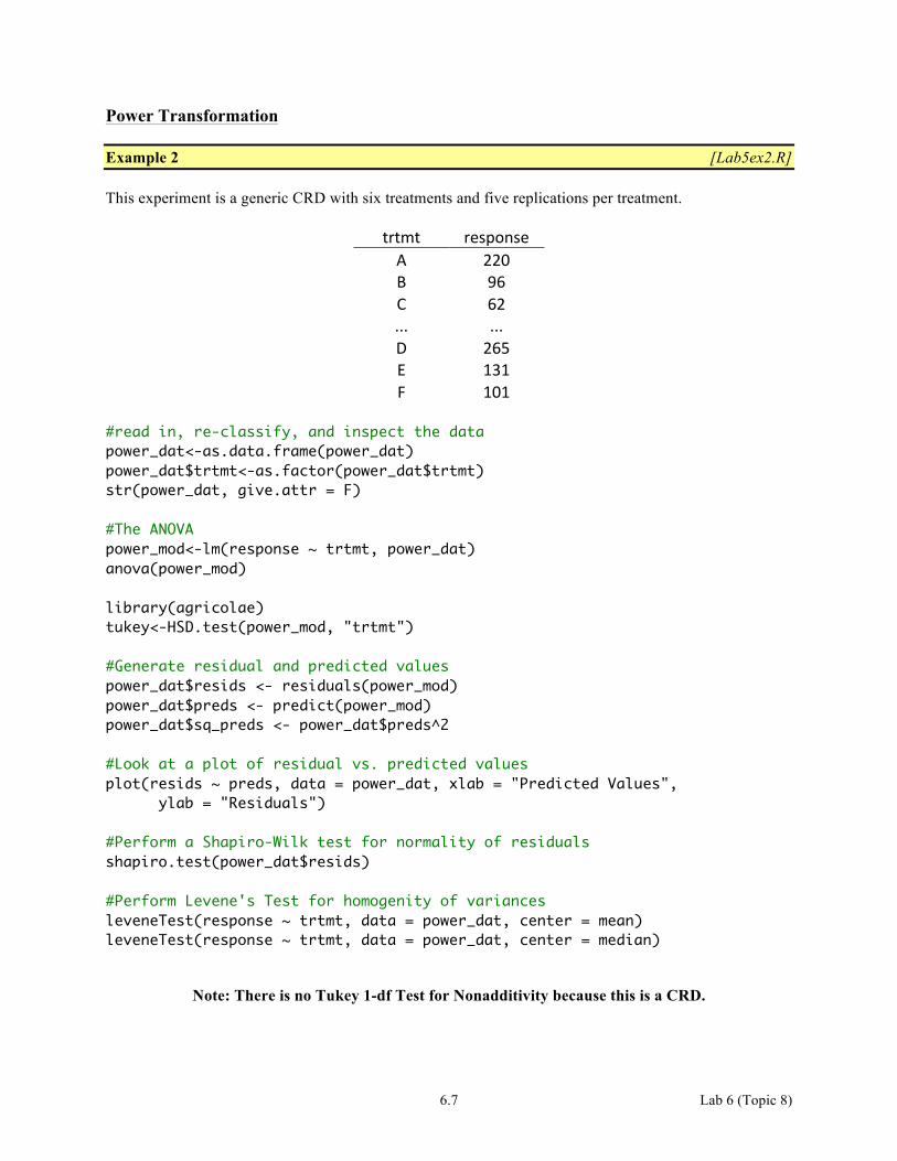
Power Transformation Example 2 [Lab5ex2.R] This experiment is a generic CRD with six treatments and five replications per treatment.

trtmt responseA 220B 96C 62... ...D 265E 131F 101

#read in, re-classify, and inspect the data power_dat<-as.data.frame(power_dat) power_dat$trtmt<-as.factor(power_dat$trtmt) str(power_dat, give.attr = F) #The ANOVA power_mod<-lm(response ~ trtmt, power_dat) anova(power_mod) library(agricolae) tukey<-HSD.test(power_mod, "trtmt") #Generate residual and predicted values power_dat$resids <- residuals(power_mod) power_dat$preds <- predict(power_mod) power_dat$sq_preds <- power_dat$preds^2 #Look at a plot of residual vs. predicted values plot(resids ~ preds, data = power_dat, xlab = "Predicted Values", ylab = "Residuals") #Perform a Shapiro-Wilk test for normality of residuals shapiro.test(power_dat$resids) #Perform Levene's Test for homogenity of variances leveneTest(response ~ trtmt, data = power_dat, center = mean) leveneTest(response ~ trtmt, data = power_dat, center = median)

Note: There is no Tukey 1-df Test for Nonadditivity because this is a CRD.

6.8 Lab 6 (Topic 8)

Output The ANOVA Df Sum Sq Mean Sq F value Pr(>F) trtmt 5 143273 28654.6 13.437 2.641e-06 *** Residuals 24 51180 2132.5 Test for normality of residuals Shapiro-Wilk normality test data: power_dat$resids W = 0.9827, p-value = 0.891 NS Test for homogeneity of variances among treatments Levene's Test for Homogeneity of Variance (center = mean) Df F value Pr(>F) group 5 2.9164 0.03396 * 24 Levene's Test for Homogeneity of Variance (center = median) Df F value Pr(>F) group 5 1.7915 0.1527

DANGER DANGER!!! Wonky Levene's Test! Transform data!

6.9 Lab 6 (Topic 8)

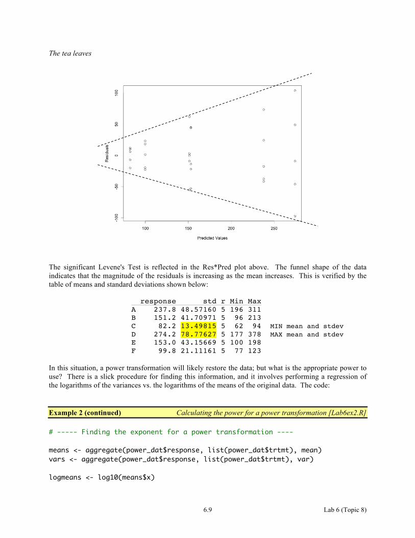
The tea leaves

The significant Levene's Test is reflected in the Res*Pred plot above. The funnel shape of the data indicates that the magnitude of the residuals is increasing as the mean increases. This is verified by the table of means and standard deviations shown below:

response std r Min Max A 237.8 48.57160 5 196 311 B 151.2 41.70971 5 96 213 C 82.2 13.49815 5 62 94 MIN mean and stdev D 274.2 78.77627 5 177 378 MAX mean and stdev E 153.0 43.15669 5 100 198 F 99.8 21.11161 5 77 123

In this situation, a power transformation will likely restore the data; but what is the appropriate power to use? There is a slick procedure for finding this information, and it involves performing a regression of the logarithms of the variances vs. the logarithms of the means of the original data. The code: Example 2 (continued) Calculating the power for a power transformation [Lab6ex2.R] # ----- Finding the exponent for a power transformation ---- means <- aggregate(power_dat$response, list(power_dat$trtmt), mean) vars <- aggregate(power_dat$response, list(power_dat$trtmt), var) logmeans <- log10(means$x)

6.10 Lab 6 (Topic 8)

logvars <- log10(vars$x) power_mod<-lm(logvars ~ logmeans) summary(power_mod) Output Coefficients: Estimate Std. Error t value Pr(>|t|) (Intercept) -2.5353 0.8463 -2.996 0.04010 * logmeans 2.5814 0.3864 6.680 0.00261 ** Locate the slope of the regression. In this case, slope = 2.5814. Now calculate the appropriate power of the transformation, where Power = 1 – (b/2). In this case,

Power = 1 – (2.5814/2) = -0.29 To use this magic number, return to R and continue coding: #Create power-tranformed variable power_dat$trans_response<-(power_dat$response)^(-0.29) #The ANOVA trans_power_mod<-lm(trans_response ~ trtmt, power_dat) anova(trans_power_mod) trans_tukey<-HSD.test(trans_power_mod, "trtmt") #TESTING ASSUMPTIONS #Generate residual and predicted values power_dat$trans_resids <- residuals(trans_power_mod) power_dat$trans_preds <- predict(trans_power_mod) #Look at a plot of residual vs. predicted values plot(trans_resids ~ trans_preds, data = power_dat, xlab = "Predicted Values", ylab = "Residuals") #Perform a Shapiro-Wilk test for normality of residuals shapiro.test(power_dat$trans_resids) #Perform Levene's Test for homogenity of variances leveneTest(trans_response ~ trtmt, data = power_dat, center = mean) leveneTest(trans_response ~ trtmt, data = power_dat, center = median)

6.11 Lab 6 (Topic 8)

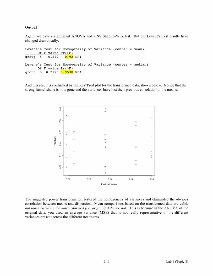
Output Again, we have a significant ANOVA and a NS Shapiro-Wilk test. But our Levene's Test results have changed dramatically: Levene's Test for Homogeneity of Variance (center = mean) Df F value Pr(>F) group 5 0.279 0.92 NS! Levene's Test for Homogeneity of Variance (center = median) Df F value Pr(>F) group 5 0.2125 0.9538 NS! And this result is confirmed by the Res*Pred plot for the transformed data, shown below. Notice that the strong funnel shape is now gone and the variances have lost their previous correlation to the means.

The suggested power transformation restored the homogeneity of variances and eliminated the obvious correlation between means and dispersion. Mean comparisons based on the transformed data are valid, but those based on the untransformed (i.e. original) data are not. This is because in the ANOVA of the original data, you used an average variance (MSE) that is not really representative of the different variances present across the different treatments.

6.12 Lab 6 (Topic 8)

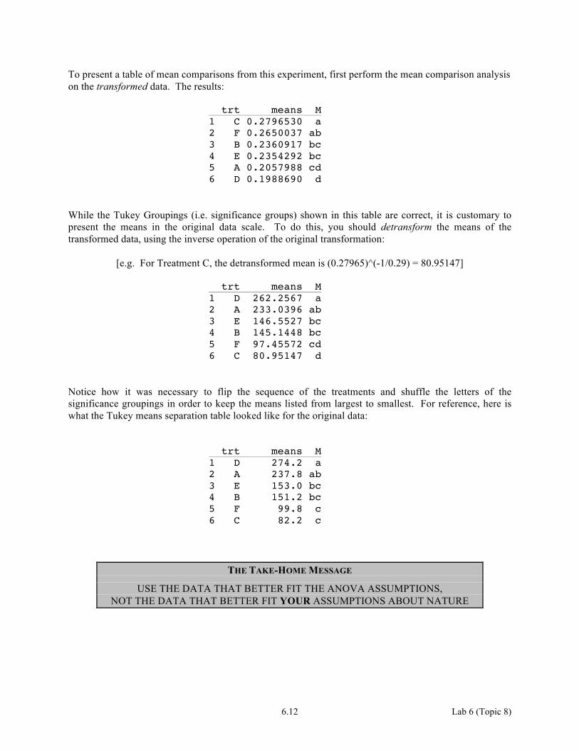
To present a table of mean comparisons from this experiment, first perform the mean comparison analysis on the transformed data. The results:

trt means M 1 C 0.2796530 a 2 F 0.2650037 ab 3 B 0.2360917 bc 4 E 0.2354292 bc 5 A 0.2057988 cd 6 D 0.1988690 d

While the Tukey Groupings (i.e. significance groups) shown in this table are correct, it is customary to present the means in the original data scale. To do this, you should detransform the means of the transformed data, using the inverse operation of the original transformation:

[e.g. For Treatment C, the detransformed mean is (0.27965)^(-1/0.29) = 80.95147]

trt means M 1 D 262.2567 a 2 A 233.0396 ab 3 E 146.5527 bc 4 B 145.1448 bc 5 F 97.45572 cd 6 C 80.95147 d

Notice how it was necessary to flip the sequence of the treatments and shuffle the letters of the significance groupings in order to keep the means listed from largest to smallest. For reference, here is what the Tukey means separation table looked like for the original data:

trt means M 1 D 274.2 a 2 A 237.8 ab 3 E 153.0 bc 4 B 151.2 bc 5 F 99.8 c 6 C 82.2 c

THE TAKE-HOME MESSAGE

USE THE DATA THAT BETTER FIT THE ANOVA ASSUMPTIONS, NOT THE DATA THAT BETTER FIT YOUR ASSUMPTIONS ABOUT NATURE

6.13 Lab 6 (Topic 8)

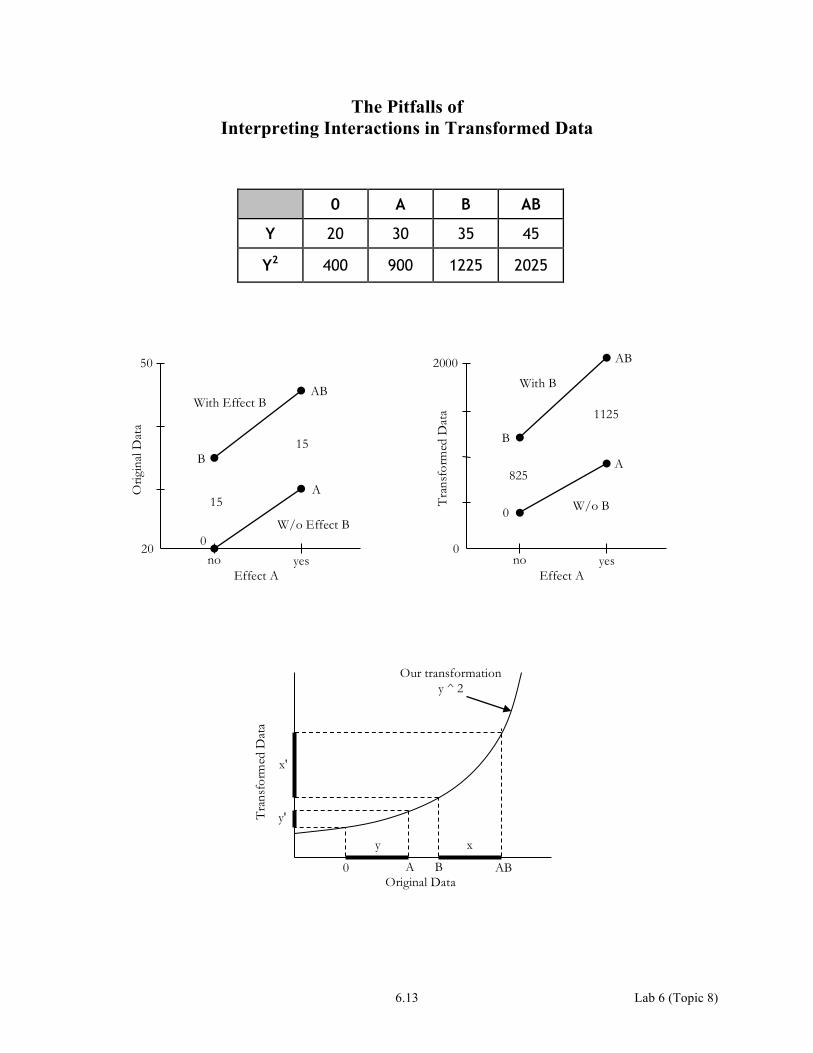
The Pitfalls of Interpreting Interactions in Transformed Data

0 A B AB

Y 20 30 35 45

Y2 400 900 1225 2025

no yes Effect A

20

50

Orig

inal

Dat

a

B

AB

A

0

With Effect B

W/o Effect B

15

15

no yes Effect A

0

2000

Tra

nsfo

rmed

Dat

a

0

AB

A

B

With B

W/o B

1125

825

Original Data

Tra

nsfo

rmed

Dat

a

Our transformation y ^ 2

B AB 0 A

x y

x'

y'