Embed Size (px)
Citation preview

04/07/2011
1
Data Warehousing and Business
Intelligence: What's Next?
Alejandro Vaisman Esteban Zimányi
Department of Computer & Decision Engineering (CoDE)
Université Libre de Bruxelles
{avaisman,ezimanyi}@ulb.ac.be
7/4/2011 BI Summer School, Paris, 2011
1
Outline
• Introduction
• Spatio-Temporal DW & BI
• Trajectory Data Warehousing & Mining
• DW & BI: New Challenges
• Real-Time DW
• DW and BI Over the Semantic Web
• Conclusion
7/4/2011 BI Summer School, Paris, 2011 2
04/07/2011
2
Outline
• Introduction
• DW & BI: New Challenges
• Spatio-Temporal DW & BI
• Trajectory Data Warehousing & Mining
• DW & BI: New Challenges
• Real-Time DW
• DW and BI Over the Semantic Web
• Conclusion
7/4/2011 BI Summer School, Paris, 2011 3
7/4/2011 BI Summer School, Paris, 2011 4
Motivation
• Location-aware devices (mobile phones and GPS, etc.) allowaccess to large spatiotemporal datasets => huge amounts of spatiotemporal data
• Need of analytical tools that transform data into knowledge
• Behavioral patterns can be found and exploited in applications likemobile marketing, traffic management etc.
• Online analytical processing (OLAP) and data mining (DM) techniques can be employed to convert raw data into usefulknowledge.

04/07/2011
3
Trajectory Data Warehousing
• Studied in the GeoPKDD project (www.geopkdd.eu)
• A Trajectory Data Warehouse (TDW) allows analyzing measures like: number of moving objects in different urban areas, average speed, speedchange, etc.
• Mining techniques can be used to discover traffic-related patterns
• Tasks & Issues• Define what we mean by TDW => characterize TDW in the context of spatio-
temporal data management
• Design (do we need a new conceptual data model?)
• Trajectory reconstruction
• ETL procedure that feeds a trajectory data warehouse with aggregatetrajectory data
• Aggregation of cube measures for OLAP purposes
7/4/2011 BI Summer School, Paris, 2011 5
7/4/2011 BI Summer School, Paris, 2011 6
Example: Traffic Analysis
• A decision support tool can analyze the behavior of people, usingdata coming from their mobile devices for
• Studying flow variations according to urban changes throughtime.
• Knowing average traveling times between different areas.
• Identifying the most popular trajectories.
• Discovering mobility patterns.
04/07/2011
4
7/4/2011 BI Summer School, Paris, 2011 7
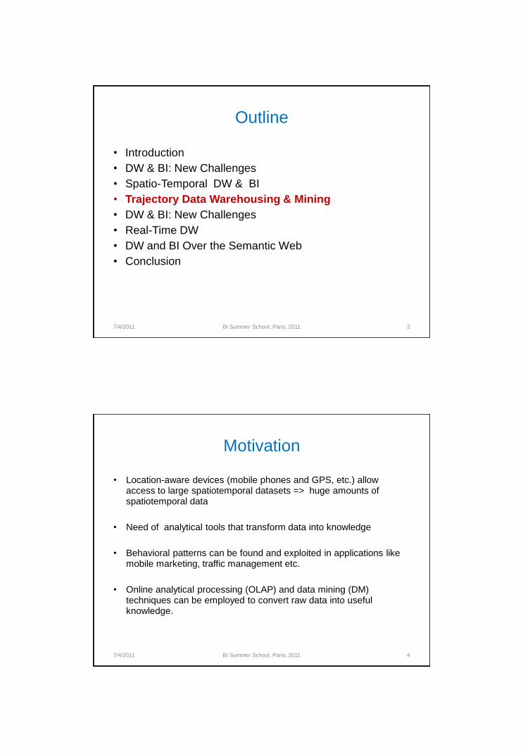
T [10min, 20min]
T [20min, 35min]
T [5min, 10min]T [25min, 45min]
Analyzing Mobile Data: Patterns
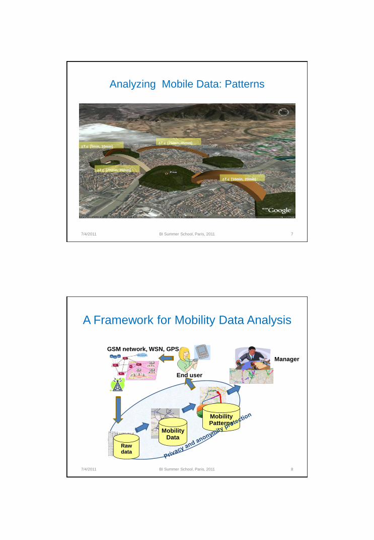
7/4/2011 BI Summer School, Paris, 2011 8
Mobility Data
Raw data
Mobility Patterns
GSM network, WSN, GPS
End user
Manager
A Framework for Mobility Data AnalysisFrom the GeoPKDD project

04/07/2011
5
7/4/2011 BI Summer School, Paris, 2011 9
Spatio-
temporal
patterns
•Spatio-temporal models for moving
objects
•Moving Object DB
•Trajectory Warehouse
•Privacy-preserving OLAP•ST data mining methods
•Data mining query languages
•Privacy-preserving data mining
Research Topics Involved
Privacy-
preserving
“skin”
Some Interesting Problems…
• How to reconstruct a trajectory from raw data, how to store and query trajectory data?
• How to classify trajectories according to means of transportation (pedestrian, private vehicle, public transportation vehicle, …)?
• Which spatio-temporal patterns and/or models are useful abstractions for mobility data? How to compute such patterns and models efficiently?
• Privacy protection and anonymity – How to find an optimal trade-off between privacy protection and quality of the analysis?
• Other problems will be addressed as we progress on this talk.
7/4/2011 BI Summer School, Paris, 2011 10

04/07/2011
6
A Trajectory Data Warehousing Architecture
7/4/2011 BI Summer School, Paris, 2011 11
As proposed in GeoPKDD
Trajectory Data Warehousing
• Characteristics of trajectories to be analyzed:
• numeric: average speed, direction, duration; etc.
• spatial: geometric shape of the trajectory;
• temporal: timing of the movement;
• Uncertainty must be considered due to raw data imprecision
• The TDW only contains aggregate information
• No trajectory information is stored
7/4/2011 BI Summer School, Paris, 2011 12

04/07/2011
7
The Trajectory Data Warehouse
• Typically, in TDW, the geographic space is divided into cells.
• Measures of interest:
• Number of trajectories found in the cell (or started/ended their path in
the cell; or crossed/entered/left the cell,…);
• {average/min/max} distance covered by trajectories in the cell;
• {average/min/max} time required to cover this distance.
• Speed and change of speed (acceleration), direction and change of
direction (turn), etc.
7/4/2011 BI Summer School, Paris, 2011 13
The Trajectory Data Warehouse
• Braz et al. [BOO+07] classify measures as:
• No pre-computation needed: the measure can be updated in the data warehouse using each single observation (e.g., trajectories starting in a cell);
• Per trajectory local pre-computation: the measure can be updatedthorugh a simple pre-computation which only involves a fewobservations of the same trajectory;
• Per trajectory global pre-computation: the measure update requires a pre-computation which considers all the observations of a single trajectory;
• Global pre-computation: the measure requires a pre-computation whichconsiders all the observations of all the trajectories.
7/4/2011 BI Summer School, Paris, 2011 14

04/07/2011
8
The Trajectory Data Warehouse
• A TDW should also support
• Spatial dimensions (e.g. coordinate, roadway, district, cell, city, province,
country)
• Temporal dimensions (e.g. second, minute, hour, day, month, year)
• Hierarchies, describing the underlying spatiotemporal framework where
trajectories move.
• Other information regarding trajectories like technographic (e.g. mobile
device used) or demographic data (e.g. age and gender of users)
7/4/2011 BI Summer School, Paris, 2011 15
Requirements and Problems
• OLAP Requirements
– A TDW Algebra should support typical OLAP operators like:
• Roll-up
• Drill-Down
• Slice & Dice
– Problem: double counting (Braz et. al., STDM‟07) which introduces
errors in the operations
7/4/2011 BI Summer School, Paris, 2011 16
Aggr(R4,R5,R6)= 3 (actual)
Aggr(R4,R5,R6)= 6 (results
from 3 + 2 +1)
Fig. from Marketos ’09

04/07/2011
9
From Raw Data to a TDW
7/4/2011 BI Summer School, Paris, 2011 17
Marketos et al, MobiDE’08
From Raw Data to the Moving Object
Database
• Steps:
• Trajectory reconstruction from raw trajectories, populates the
MOD
• ETL feeds the data cub with pre-aggregated data
• OLAP & Mining allow exploiting the trajectory data cube
• Typical MOD schema
– OBJECTS (id: identifier, description: text, gender: {M | F}, birth-date:
date, profession: text, device-type: text)
– RAW_LOCATIONS (object-id: identifier, timestamp: datetime, x-pos:
numeric, y-pos: numeric, altitude-z: numeric)
– MOD_TRAJECTORIES (trajectory-id: identifier, object-id: identifier,
trajectory: 3D geometry)
7/4/2011 BI Summer School, Paris, 2011 18

04/07/2011
10
Trajectory Reconstruction
• Raw data come in bulk streams
• When does a trajectory start and end?
• temporal gap (maximum time gap between two points in the same
trajectory)
• spatial gap (maximum spatial distance between two points)
• Maximum speed (used to detect noise)
• Maximum noise duration (sequence of noisy observations => a new
trajectory)
• Tolerance distance D (if two observations are closer than D, the latest
one is considered redundant)
7/4/2011 BI Summer School, Paris, 2011 20
Trajectory Reconstruction
7/4/2011 BI Summer School, Paris, 2011 21
F. Braz, BSG ’07
• Lack of observations in a cell (add interpolated points)
• More than one observation in a cell (remove duplicates)
• The double count problem arises not only during aggregation of the
base data during a roll-up operation, but also in the loading phase.
For example, suppose we have three consecutive observations o1,
o2, o3. o1 falls in cell1, o2 in cell2, o3 in cell1 => o1 and o3
contribute to the presence in Cell1, although only one should be
counted.

04/07/2011
11
A Trajectory Data Warehouse
7/4/2011 BI Summer School, Paris, 2011 22
Marketos et al. , MobiDE’08
A Trajectory Data Warehouse
• The spatial dimension can be defined in many ways (grids, road
networks, mobile telephony cells, etc). Our example asumes a grid
(size of the cells is a parameter of the process)
• Temporal granularity depends on the application
• Fact table contains the key of the dimension tables, and a set of
measures including aggregate information for a particular group of
people moving in a specific spatial area during a specific time
period:
– number of distinct trajectories ( COUNT_TRAJECTORIES)
– number of distinct users (COUNT_USERS)
– average traveled distance (AVG_DISTANCE_TRAVELED)
– average travel duration (AVG_TRAVEL_DURATION)
– average speed (AVG_SPEED)
7/4/2011 BI Summer School, Paris, 2011 23

04/07/2011
12
The Presence Measure
7/4/2011 BI Summer School, Paris, 2011 24
• Studied in (Orlando et al., DaWak 2007)
• Strategies for approximating the results of computing the pre-aggregated
facts
• Linear interpolation used to prevent omitting the cells crossed by a
rajectory but s.t. no sampling occurred within them.
• The authors address the problem of double counting during aggregation
borrowing from statistical methods.
• Example:• Presence for two neighbour cells, Cx,y and Cx+1,y is known
• A new cell, Cx‟,y‟= Cx,y U Cx+1,y, is defined
• Aggregate presence over the new cell, will be:
Cx’,y’.presence = Cx,y.presence + Cx+1,y.presence - Cx,y.crossX
Cx,y.crossX is the number of distinct trajectories crossing the spatial border
between Cx,y and Cx+1,y.
Semantic Issues
7/4/2011 BI Summer School, Paris, 2011 25
• Trajectory analysis based on requirements of different stakeholders• Ex: a traffic analyst and a logistics manager view trajectories in different
ways.
(a) Raw data; (b) Logistics view (c) Traffic analyst view (d) Compressed
traj. => Marketos & Theodoridis (MDM 2010) propose an ad-hoc OLAP
framework

04/07/2011
13
Exploiting the TDW
7/4/2011 BI Summer School, Paris, 2011 26
• Leonardi et al. (2010) presentted T-Warehouse . Based on the
concepts explained (architecture. double counting, presence, etc.)
• Allows analyzing trajectory data at different levels of aggregation
• Velocity and presence graphic. Triangle base: presence; triangle height:
velocity
Exploiting the TDW
7/4/2011 BI Summer School, Paris, 2011 27
• Another visualization style: Presence on Tuesday (base granurarity
level)

04/07/2011
14
7/4/2011 MDM 2010, Kansas City, Misouri 28
Exploiting the TDW • Time Graph for Presence during a week. Each curve corresponds to a cell.
Open Questions…
• How is the DW efficiently maintained?
• How are dimensions updated?
• What happens if we want to modify the grid size? => recompute
• How do we really obtain NEW and UNKNOWN information?
7/4/2011 BI Summer School, Paris, 2011 29

04/07/2011
15
7/4/2011 BI Summer School, Paris, 2011 30
Trajectory Querying
• The nature of trajectory data provides us with the ability to query them with
a variety of operators
– Coordinate-based
– Trajectory-based
– Similarity-based
– Motion pattern queries
7/4/2011 BI Summer School, Paris, 2011 31
Trajectory Mining
• Data mining tasks: association, classification, clustering, pattern
recognition….
• For trajectories, these tasks can imply:
• Clustering: discovery of similar trajectories in terms of similarity measures
• Frequent patterns: frequent sub-paths in trajectories
• Classification: behavioral rules for predicting future movements
• Interaction patterns

04/07/2011
16
7/4/2011 BI Summer School, Paris, 2011 32
Trajectory Mining
• Patterns
– T-patterns
– Periodic patterns
– Relative motion
– Flock
– Leadership
– Convergence
– Encounter
– Hot motion
• Clustering
– Probabilistic
– Density-based
• Regular expression-based patterns
7/4/2011 BI Summer School, Paris, 2011 33
Trajectory Mining
• Patterns
– T-patterns
– Periodic patterns
– Relative motion
– Flock
– Leadership
– Convergence
– Encounter
– Hot motion
• Clustering
– Probabilistic
– Density-based
• Regular expression-based patterns

04/07/2011
17
7/4/2011 BI Summer School, Paris, 2011 35
T-Pattern (Giannotti et al., KDD ‟07)
• A sequence of regions, frequently visited in a specified order with
similar transition times
7/4/2011 BI Summer School, Paris, 2011 36
Trajectory Pattern - Definition
• A Trajectory Pattern (T-pattern) is a pair (s,α):
– s = <(x0,y0),..., (xk,yk)> is a sequence of k+1 locations
– α = <α1,..., αk> are the transition times (annotations)
• A T-pattern Tp occurs in a trajectory if the trajectory contains a
subsequence S such that:
– Each (xi,yi) in Tp matches a point (xi‟,yi‟) in S, and
the transition times in Tp are similar to those in S
α2

04/07/2011
18
7/4/2011 BI Summer School, Paris, 2011 37
T-Patterns
• Routes between two consecutive regions are not relevant
• Absolute times are not relevant
A B
1 hour
1 hour
A B
These movements cannot be distinguished using T-patterns
1 hour at 5 p.m.
1 hour at 9 a.m.
7/4/2011 BI Summer School, Paris, 2011 3838
Approach 1: predefined regions
• Fix a set of pre-defined regions of interest
• Map each (x,y) of the trajectory to its region
• Sample pattern:MallstationBus .min20
time
Bu
s s
tati
on
Parking
Mall

04/07/2011
19
7/4/2011 BI Summer School, Paris, 2011 3939
Approach 2: static discovered regions
• Detect significant regions thru spatial clustering
• Map each (x,y) of the trajectory to its region
• Sample pattern:),(),( 22
.min20
11 yxaroundyxaround
time
around(x1,y1)
around(x1,y1)
7/4/2011 BI Summer School, Paris, 2011 40
Approach 3: dynamically discovered regions
• Dynamic discovering of dense regions Regions are defined at each step of the pattern generation
• Sample pattern:ByxAyx ),(),( .min20
1.Considering all trajectories, A
is a cluster / dense region
2.Considering only trajectories
that visit A, B is a cluster
3.”20 mins” is a typical time for
pattern ABx
y
(x1,y1)
(x2,y2)
(x3,y3)
(x4,y4)
t = 20 min.A
B

04/07/2011
20
7/4/2011 BI Summer School, Paris, 2011 41
Trajectory Clustering
• Adapts the classic data mining task to the discovery of groups
of similar trajectories.
• Spatio-temporal trajectory data introduces some questions:
– Which distance between trajectories?
– Which kind of clustering?
7/4/2011 BI Summer School, Paris, 2011 42
• Average Euclidean distance between trajectories:
• “Synchronized” behaviour distance
– Similar objects = likely to be in the same place at the same time
• Computed on the whole trajectory
• Computational aspects:
– Cost = O( |1| + |2| ) (|| = number of points in )
– It is a metric => efficient indexing methods allowed, e.g.
(Frentzos et al. 2007)
||
))(),((|),(
21
21T
dtttdD T
T
A Distance Function
distance between moving
objects 1 and 2 at time t
(Nanni and Pedreschi, JIIS‟ 06)

04/07/2011
21
7/4/2011 BI Summer School, Paris, 2011 43
Kind of Clustering
• General requirements:
– Non-spherical clusters should be allowed
– Tolerance to noise
– Low computational cost
– Applicability to complex, possibly non-vectorial data
• A suitable candidate: Density-based clustering
• Key idea of density-based clustering: for each object in some cluster the
neighborhood of a given radius e has to contain at least a minimum number
of objects
• Nanni & Pedreschi extend OPTICS (Ankerst et al., 1999) yielding
T(rajectory)-OPTICS
7/4/2011 BI Summer School, Paris, 2011 46
Progressive clustering
• Visually-driven clustering is used to analyze data
• Based on a progressive refinement of the solution through visually-driven
exploration, applying increasingly complex similarity functions
• For example, first create a large cluster of trajectories using a “common
ends” distance function. Then, refine by creating subclusters using a more
sophisticated distance function (e.g.,route similarity)

04/07/2011
22
7/4/2011 BI Summer School, Paris, 2011 47
Interactive density-based trajectory clustering
(Rinzivillo et al., J. of Information Visualization, 2008).
7/4/2011 BI Summer School, Paris, 2011 48
The Milano Example

04/07/2011
23
7/4/2011 BI Summer School, Paris, 2011 49
Dark grey: moves occurring in trajectories from several clusters
Five Biggest Sub-clusters Towards the City
Center
7/4/2011 BI Summer School, Paris, 2011 50
Left: peripheral routes; middle: inward routes; right: outward routes.
Clustering Trajectories on “Route Similarity”(Rinzivillo et al., 2008

04/07/2011
24
7/4/2011 BI Summer School, Paris, 2011 51
Trajectory Data Mining Applications Need...
• Reasoning on a richer form of knowledge about mobility
– Geographic semantics
– Landmarks and interesting places
– Categorization of such places (ontologies, OLAP
hierarchies?...)
– Road network
– Landscape
– …
– Movement sematics
– Stops and moves
– Purposes of movement
– means of transportation
– …
7/4/2011 BI Summer School, Paris, 2011 53
Semantic Trajectories
• Trajectories are given in the form (Oid,x,y,t)-tuples. Assume they are stored in a relational table called MOFT.
• Usually, no semantic information given.
• The notion of Places of Interest allows replacing a trajectory by a temporally ordered sequence of Stops and Moves.
• The encoded trajectory, plus the additional geographic information, define a Semantic Trajectory (Alvarez et al., ACM-GIS 2007, Spaccapietra et al., 2008).

04/07/2011
25
7/4/2011 BI Summer School, Paris, 2011 54
Semantic Trajectories
• t-patterns are defined by extension.
• Gomez & Vaisman (EDBT‟ 09) generalize patterns, encapsulating them as REs, and apply these REs to Semantic Trajectories. That is, extend the notion of t-pattern, defining patterms using regular expressions overplaces of interest.
• Previous work on RE over Places of Interest (Gomez et al., SAC 2008, Annals of IS, 2008)
• Visit http://piet.exp.dc.uba.ar/mo-patterns
7/4/2011 BI Summer School, Paris, 2011 55
Places of Interest - Stops and Moves
In RC1, RC4 , initial and final points are far enough from
each other => a stop.
Between Rc1 and Rc4 there is a move.
RC2, RC3 PoIs but not stops.

04/07/2011
26
7/4/2011 BI Summer School, Paris, 2011 56
Places of Interest - Stops and Moves
7/4/2011 BI Summer School, Paris, 2011 57
Stops and Moves (MOFT & SM-MOFT)

04/07/2011
27
7/4/2011 BI Summer School, Paris, 2011 58
Semantically Similar Trajectories
7/4/2011 BI Summer School, Paris, 2011 59
Semantically Similar Trajectories

04/07/2011
28
7/4/2011 BI Summer School, Paris, 2011 60
Regular Expression-Based Patterns
• Use the notion of semantic trajectories
• Define patterns in terms of stops-and-moves
• Regular expressions first used to express mobility patterns by du Mouza &
Rigaux (2004)
• Gomez & Vaisman (EDBT „09) use regular expresions to prune the
outcome of the mining process => RE over semantic trajectories.
7/4/2011 MDM 2010, Kansas City, Misouri 61
• Constraints without variables
– Trajectories that visit a cheap place during the third quarter of any year.
[rollup(ts_date, “quarter”, “Time”)=“Q3” price=“cheap”]
Note: This query uses a rollup function over a Time dimension.
– trajectories of tourists who visit hotel H1 and then a cheap place or a place serving French food.
[ID=“H1”].([price=“cheap”]|[typeOfFood=“French”])
Regular Expression-Based Patterns

04/07/2011
29
7/4/2011 MDM 2010, Kansas City, Misouri 62
• Constraints with variables
– Trajectories that start at a pla ce characterized by price, and then stop
either at the zoo or the Eiffel Tower. After this, they stop at a place that
serves French food and has the same price range as the initial stop.
[price=@x].( [ID=“Z”] | [ID=“E”]).[typeOfFood=“French” price=@x]
– Trajectories that stopped at two places (the second one having cheap
prices), at the same part of the day (e.g., both of them during the
morning), on 10/10/2008.
[rollup(ts_time, “range”, “Time”)=@z
ts_date=“10/10/2008”].[rollup(ts_time, “range”, “Time”)=@z
ts_date=“10/10/2008” price=“cheap”]
Regular Expression-Based Patterns
Outline
• Introduction
• Spatio-Temporal DW & BI
• Trajectory DW and Mining
• DW & BI: New Challenges
• Real-Time DW
• DW and BI Over the Semantic Web
• Conclusion
7/4/2011 BI Summer School, Paris, 2011 63

04/07/2011
30
• Enormous amounts of data from a wide variety of domains
– Semantic web
– Biological
– Image and video
– Genomic
….
• Traditional approach, where organizational data collected in a
huge common repository through complex ETL process, is not
appropriate for these new application domains.
• ETL processes take long time to refresh; difficult to add/delete
sources. Shorter time windows for the process. Need to be up-to-
date.
7/4/2011 BI Summer School, Paris, 2011 64
New Scenarios
• Cohen et al. (VLDB, 2009) propose dramatic changes to this
process: the MAD Skills approach:
– (M)agnetic: attract new sources
– (A)gile: allow agile evolution
– (D)eep: new kinds of analysis
– “Model less, iterate more” approach
– ELT vs ETL: load as much and as fast as possible
7/4/2011 BI Summer School, Paris, 2011 65
New Scenarios

04/07/2011
31
• Stonebraker (CACM, 2011) suggests 10 ideas for modern DW:
– Star & Snowflake schema will survive
– Column stores will dominate the DW market
– DW not appropriate for main/flash memory DBs
– Massively Parallel Processors (MPP) will be a must
– Process automation required to reduce the DB
administration costs
– Appliances: “software only” (i.e., no specialized HW)
– Keep hybrid workloads separated
– High availability required
– Online reprovisioning for adjusting load changes
– Avoid virtualization for DW if possible
7/4/2011 BI Summer School, Paris, 2011 66
New Scenarios
• New architectures gaining momentum
– Parallelism
– MapReduce programming model being also used for DW in
spite of problems processing joins, e.g., Facebook DW built
with Hadoop (Thusho et al., ICDE 2010, SIGMOD 2010)
• Must deal with new kinds of data, complex in structure and semantics
• New models and requirements for
– Spatial and Spatio-temporal BI
– Real-time DW
– Semantic Web DW & OLAP
– We will discuss them in this presentation...
7/4/2011 BI Summer School, Paris, 2011 67
New Scenarios

04/07/2011
32
Outline
• Introduction
• Spatio-Temporal DW & BI
• Trajectory Datawarehousing & Mining
• DW & BI: New Challenges
• Real-Time DW
• DW and BI Over the Semantic Web
• Conclusion
7/4/2011 BI Summer School, Paris, 2011 68
Real-Time DW
7/4/2011 BI Summer School, Paris, 2011 69
• Data Warehousing Systems are complex environments
• Data record lifecycle
• Starts with a business event
• Event record delivered to the DW
• Transformation & cleanup
• Business decision
• Consequence: data latency
• Business require real-time data
• Data acquisition time must be minimized
• Real-time DW needed
BIRTE: Workshop on Enabling Real-Time for Business Intelligence (6th
edition, 2011)

04/07/2011
33
Real-Time DW
7/4/2011 BI Summer School, Paris, 2011 70
• Examples (Schneider 2006)
• Collaborative filtering, e.g., with queries such as ``People who like X also like Y'' : Timeliness in the range of hours;
• Fraud Detection. Detects anomalies in credit card usage.Timeliness in the order of minutes;
• Call Center applications. Provide next best offer or action.Timeliness is again, minutes.
• Web Page Usage (page views, ad views, link views, clicks) by property, geography, user demographics, etc. Timeliness: hours
• Business Activity Monitoring and Operational Performance Management consists (e.g., real-time inventory analysis) Timeliness in the order of minutes.
Real-Time DW
7/4/2011 BI Summer School, Paris, 2011 71
• Goal: reduce data latency
• Main Challenges
• Data scales
• Performance
• Low latency data delivery
• Consistent response time
• Caching
• Cost. Performance/low-latency is very expensive
• High Availability: Servers, network, databases, middleware,
applications

04/07/2011
34
Real-Time DW
7/4/2011 BI Summer School, Paris, 2011 72
• Data latency reduced at the expense of probable data inconsistency (late,
missing data), high availability requirements, SQL extensions needed for
streaming operations.
• Many applications willing to pay very low data latency.
• Some applications do still NOT require latency in the seconds granularity.
For example (e.g., may demand for less “fresh” data).
• In the latter case, common evolution strategy is to increase frequency of
ETL operations using mini-batch ETL, e.g., load data every 10 minutes.
Challenges
• Enable Real-Time ETL
• Modeling Real-Time Fact Tables
• Allow OLAP queries while updating data
• Scaling the solution
Langseth, J., "Real-Time Data Warehousing: Challenges and Solutions", DSSResources.COM,
02/08/2004.
7/4/2011 BI Summer School, Paris, 2011 73

04/07/2011
35
Challenges
• Enable real-Time ETL
• Near Real Time
• Direct Trickle Feed
• Trickle & Flip
• External Real-Time data cache
7/4/2011 BI Summer School, Paris, 2011 74
Direct Trickle Feed
• Continuously feed the data warehouse with new data from the source system.
• Done by either directly inserting/updating data in the fact tables, or by inserting data into separate fact tables in a real-time partition.
• Real-time data loading packages t specifically designed for this (DataMirror, MetaMatrix, etc.).
• Java Messaging Service (JMS) used to transmit each new data element from the source system to a lightweight listener application that in turn inserts the new data into the warehouse tables.
• Problem : doesn't scale well even under moderate query use. (mixed workload problem): Constantly updating tables that are being queried by an OLAP tool degrades performance
Opposed to Stonebraker's recommendation (CACM,2011).
7/4/2011 BI Summer School, Paris, 2011 75

04/07/2011
36
Trickle & Flip
7/4/2011 BI Summer School, Paris, 2011 76
• The "Trickle & Flip" approach addresses the mixed workload problem o
• Instead of loading the data in real-time into the actual warehouse tables, the
data is continuously fed into staging tables that are in the exact same format as
the target tables.
• Staging tables either contain a copy of just the data for the current day, or (for
small fact tables), a copy of ALL the historical data.
• Periodically the staging table is duplicated and the copy is swapped with the
fact table, bringing DW up-to-date. (stopping the OLAP server while flipping
is recommended).
• Cycle times ranging from hourly to every minute. Best performance: 5-10
minute cycles
.
Real-Time Data Cache
7/4/2011 BI Summer School, Paris, 2011 77
• The RTDC be another dedicated database server (or a separate instance
of a large database system) dedicated to loading, storing, and processing
the real-time data.
• In-Memory DB for RTDC for large volumes of real-time data (hundreds
or thousands of changes per second), or extremely fast query
performance requirements
• All the real-time data is loaded into the cache as it arrives from the source
system. Either all queries that involve the real-time data are directed to
the RTDC, or RT data is seamlessly imaged to the DW

04/07/2011
37
Challenges
7/4/2011 BI Summer School, Paris, 2011 78
• Modeling Real-Time Fact Tables
• Model as usual with Direct FT feed
• Separate RT partitions - RT and historical data stored in separa fact
tables (Kimball,2002 - “RT Partitions”). Query tools should be able to
distinguish both kinds of table, and know where to find data. More
complex to build.
• Integrate RT using Views- - RT data stored in separate tables but with the
SAME table structure. Combined through views to look as a single one.
• Modeling with an external Real-Time data cache. No new modeling
required. RDTC has the same structure as historical data.
Challenges
7/4/2011 BI Summer School, Paris, 2011 79
• Allow OLAP Querying While Updating Data
• Problem: Relational OLAP tools evaluate queries issuing multi-pass SQL
statements over temporary tables. Many of these queries takes longer than
the accepted latency for RTDW (i.e., fdata changes during query execution).
Consequence: inconsistency or unacceptable response times.
• Solutions:
• Near RT, not issuing OLAP queries while feeding data
• Risk mitigation. Separate complex queries from the workload.
• Using external RTDC completely separating RT from historical data

04/07/2011
38
Challenges
7/4/2011 BI Summer School, Paris, 2011 80
• Scaling the Solution
• Simplify and limit RT reporting
• Add computing power. Parallel RDBMS, other parallel systems
solutions based on adding computing nodes (MapReduce model)
• Using RTDC. Does not work well sometimes: if RT data is external to
the warehouse, complex to include in single report or analysis real-
time and historical information.
• Just in Time Information Merging” (JIM) approach. RT data introduced
and merged in the DW when needed. A JIM-RA (request analizer)
determines the RT data. Then another component takes a snapshot
image of these parts, and loads it into temporary tables in the DW.
Them, JIM-RA modifies the original query to include the temporary
tables containing the snapshot data.
Change Data Capture (CDC)
7/4/2011 BI Summer School, Paris, 2011 81
• Architectures for collecting transactional data from operational
sources vary mostly on the latency of data integration, from
daily batches to continuous real-time integration.
• The capture of data from sources is either performed through
incremental queries that filter based on a timestamp or flag
or...
• Through a CDC mechanism that detects any changes as it is
happening.
• Architectures are further distinguished between pull and push
Operation.
Pull: polls in fixed intervals for new data
Push: Data is loaded into the target once a change
appears.
•

04/07/2011
39
Architectures for CDC1
7/4/2011 BI Summer School, Paris, 2011 82
1. From “Best Practices for Real-time Data Warehousing”. Oracle White Paper, May, 2010.
RiTE: Right Time DW
7/4/2011 BI Summer School, Paris, 2011 83
• Proposed by Thomsen, Pedersen Lehner (ICDE, 2008)
• Need for a solution that makes inserted data available quickly, while still
providing bulk-load insert speeds.
• Based on the fact that parts of the data must be loaded quickly after arrival,
while other parts can be loaded at regular intervals.
• Right-time data warehousing'', opposite to ``near-real time DW'', were data is
loaded into the DW minutes or seconds after it arrives.
• In both approaches, regular SQL INSERT statements are used, leading to
slow insert speed.
• A solution: Find the correct batch size between the two extremes (bulk load
vs. single-row INSERT).

04/07/2011
40
RiTE: Right Time DW
7/4/2011 BI Summer School, Paris, 2011 84
• A data producer scontinuously inserts data into a DW at bulk-load
speed
• Data consumers (DW clients executing queries) get access to
fresh data.
• RiTE is targeted at supporting one producer (the ETL program)
doing many INSERTs with low persistency requirements.
• A main-memory based catalyst that enables the insert process to
be performed faster and with less effort.
• Using RiTE is transparent and requires only very few changes to
producer and consumer code.
RiTE: Right Time DW
7/4/2011 BI Summer School, Paris, 2011 85

04/07/2011
41
RiTE: Right Time DW
7/4/2011 BI Summer School, Paris, 2011 86
• The RiTE architecture includes:
• An specialized JDBC database driver for the producer
• An specialized JDBC database driver for the consumers
• A main-memory “catalyst” that provides intermediate storage (“memory
tables”) for (user-chosen) DW tables.
• Offers fast insertions and concurrency control.
• Data can be queried while held by memory tables, transparently to the end user.
• Eventually data moved to its final target –the physical DW tables
• A PostgreSQLtable function makes the data available in the DW
RiTE: Right Time DW
7/4/2011 BI Summer School, Paris, 2011 87
Producer Operations• The two producer operations insert and commit are handled specially by
RiTE. From the user's point of view, insert operations work as normal
inserts but are faster.
• RiTE temporarily keeps the inserted values locally at the producer side
and later moves them towards the DW in bulk.
• When to move data in bulk is decided based on the concept that such
that the data always is available from the DW when it is needed for
querying.
• Commit operation makes inserted data available for consumers. The
user decides if committed data is written to the DW's tables. If this is
done, the commit is called a materialization. If the user does not have
strict persistency requirements (e.g., if the data can be re-extracted from
the sources), it is also possible to commit the data without doing a
materialization (can be done later)

04/07/2011
42
RiTE: Right Time DW
7/4/2011 BI Summer School, Paris, 2011 88
-
Consumer Operations
• Two operations: read and ensure accuracy.
• From the user's point of view, a read is done by using SELECT.
• Transparently to the user, the read is not necessarily just a read from
tables in the DW.
• The only new operation introduced by RiTE is ensure accuracy.
• If a consumer that does not necessarily need fresh data (helping the
system to get a better performance, using the ensure accuracy operation,
the consumer is guaranteed that it at least sees the data that existed e.g.,
10 minutes ago.
RiTE: Right Time DW
7/4/2011 BI Summer School, Paris, 2011 89
-
Catalyst
• Purpose: provide fast, intermediate storage for data
• Stores rows in main memory.
• It can serve one producer driver and many consumer drivers and their
table functions at the same time.
• Note that the consumer driver itself does not fetch rows. Instead it
(transparently to the user) informs the catalyst about which rows should
be readable by a table function. A table function makes rows accessible in
the DW.
• Functions: (1) store rows for a producer; (2) deliver them to a table
function, and (3) delete them when they are marked as unused (i.e., no
consumer currently uses them and they have been materialized).

04/07/2011
43
Industry Tools: ODI (Oracle Data Integrator)
7/4/2011 BI Summer School, Paris, 2011 90
-
Push and suscribe strategy: 1. An identified subscriber (e.g., an integration process) subscribes to changes that
might occur in a datastore.
2. The Changed Data Capture framework captures changes in the datastore and then
publishes them for the subscriber.
3. The subscriber can process the tracked changes at any time and consume these events.
Once consumed, events are no longer available for this subscriber.
7/4/2011 BI Summer School, Paris, 2011 91
-
Industry Tools: ODI (Oracle Data Integrator)
- Non-invasive strategy
- Process log files of completed transactions and stores these captured changes into external Trail
Files independent of the database.
- Changes are transferred to a staging database.
- Processes detected changes in the staging area.
- Changes loaded into the target data warehouse using ODI‟s declarative transformation mappings.
- Architecture enables separate real-time reporting on the normalized staging area tables in addition to
loading and transforming the data into the analytical data warehouse tables.

04/07/2011
44
7/4/2011 BI Summer School, Paris, 2011 92
Greenplum
Outline
• Introduction
• DW & BI: New Challenges
• Spatio-Temporal DW & BI
• Trajectory Data Warehousing & Mining
• DW & BI: New Challenges
• Real-Time DW
• DW and BI Over the Semantic Web
• Conclusion
7/4/2011 BI Summer School, Paris, 2011 93

04/07/2011
45
DW on the Semantic Web
• The Semantic Web (SW) is a proposal oriented to represent Web content in an easily machine-processable way.
• The basic layer of the data representation for the Semantic Web recommended by the World Wide Web Consortium (W3C) is the Resource Description Framework (RDF)
• The Ontology Web Language (OWL) is a language for the specification of ontologies, whose definition by the W3C Consortium has encouraged different communities to develop large and complex ontologies like the NCI thesaurus, GALEN, etc
• OWL provides a powerful knowledge representation language with well defined semantics based on Description Logics (DL).
• Large repositories of semantically annotated data will be available, opening new opportunities for enhancing current decision support systems.
7/4/2011 BI Summer School, Paris, 2011 94
RDF
7/4/2011 BI Summer School, Paris, 2011 95
-• The standard of the W3C for representing metadata on
the Web
• RDF conceptual base is (following W3C documents):
• Graph data model
• URI-based vocabulary
• Datatypes
• XML serialization syntax
• Expression of simple facts
• Entailment

04/07/2011
46
RDF
7/4/2011 BI Summer School, Paris, 2011 96
-
From a database point of view:
• A data representation language with a graph-like structure
(resembling semantic networks)
• A notion of anonymous representation (existential variables) called
blank nodes (B)
• A set of reserved words (RDF Schema) with predefined semantics
(subclassing, typing).
•A notion of entailment.
RDF Triple: (v1,v2,v3) -> (subj,pred,obj)
Subject: URI or B
Predicate: URI
Object: URI or B or Literal (L)
RDF graph: a set of RDF triples
An RDF Graph
7/4/2011 BI Summer School, Paris, 2011 97
-
From Gutierrez et al. (PODS 04)

04/07/2011
47
Two Main Lines of Work
7/4/2011 BI Summer School, Paris, 2011 98
-• Automatic design of DW from ontologies
• Analysis of Semantic Web data
Automatic DW Design
7/4/2011 BI Summer School, Paris, 2011 99
-
• Niinimaki and Niemi (JoDS, 2009) use semantic web
technologies to populate OLAP cubes. They use ontology
mapping to convert data sources to RDF and then query RDF
data with SPARQL to Populate the OLAP schema. For this, they
use an OLAP ontology (i.e., an ontology that explains the DW
model)
• Romero and Abelló (DOLAP,2007) address the design of the
data warehouse starting from an OWL ontology that describes
the data sources. They identify the dimensions that
characterize a central concept under analysis (the fact concept)
by looking for concepts connected to it through one-to-many
relationships. The same idea is used for discovering levels of
the dimension hierarchies, starting from the concept that
represents the base level. Output: Star or Snowflake schema
that guarantees summarizability.

04/07/2011
48
Analyzing Ontology Instances
7/4/2011 BI Summer School, Paris, 2011 100
-
• Nebot et al. (JoDS,2009) define a Semantic Data Warehouse
(SDW) as a semi-structured repository consisting of
semantic annotations along with their associated set of
ontologies,
• Introduce the Multidimensional Integrated Ontology (MIO) as a
method for designing, validating and building OLAP-based cubes
for analyzing the stored annotations.
• Propose a framework for designing multidimensional analysis
models over the semantic annotations stored in a SDW
Extracting SW Data
7/4/2011 BI Summer School, Paris, 2011 101
-
-
• Nebot et al., EDBT Workshops,2010
• Like an ETL process for Semantic Web data
• SW data consists in axioms and annotations relating instances
• Data separated into schema -called the “ontology” (Tbox) e
Instances- called “semantic annotations” (ABox)
Instances are triples where the predicate is a property

04/07/2011
49
7/4/2011 BI Summer School, Paris, 2011 102
-
Extracting SW Data
Transforming an Ontology into MD Data
7/4/2011 BI Summer School, Paris, 2011 103
-

04/07/2011
50
7/4/2011 BI Summer School, Paris, 2011 104
-
Extracting SW Data - Architecture
7/4/2011 BI Summer School, Paris, 2011 105
-The fact extractor is based on the notion of
contexts (least common reachable instance)
Extracting SW Data

04/07/2011
51
7/4/2011 BI Summer School, Paris, 2011 106
-
From Ontology to DW Fact Tables
7/4/2011 BI Summer School, Paris, 2011 107
-
From Ontology to DW Fact Tables
04/07/2011
52
Scalable Analysis of SW Data
7/4/2011 BI Summer School, Paris, 2011 108
-
• Semantic web data represented as RDF triples, modeled
as a labeled graph
• Analytical queries consist of three main constructs:
pattern Matching, grouping and aggregation. That means,
join operations are needed to transform data into n-ary
relations relevant to the given query.
• Different than traditional OLAP data structures.
• Processing joins on semantic web data implies that
powerful processing mechanisms are needed, like
parallel programming tools.
• Parallel processing systems, based on Shared-nothing
architectures increasingly used to process scalable
analytical workloads (Stonebraker & Catell, 2010).
7/4/2011 BI Summer School, Paris, 2011 109
-
• Parallel systems not optimized for relational algebra
Operations. Designed to work on an homogeneous dataset,
penalize joins. HadoopDB aimed at solving this problem.
However, RDF processing requires a high number of joins.
-
-
• MapReduce programming model
• Tasks encoded in two functions: Map & Reduce
• Map transforms data into <key,value> pairs
• Keys sorted and merged
• Objects with the same key collected by a reducer
• Reducer performs aggregation
Scalable Analysis of SW Data

04/07/2011
53
7/4/2011 BI Summer School, Paris, 2011 110
-
From Sridhar et al (ISWC,2009)
Scalable Analysis of SW Data
7/4/2011 BI Summer School, Paris, 2011 111
-
• Even for the simple sales data of previous slide analytical queries
are very complex, usually requiring multiple aggregations over
multiple groups of data.
“Total sales amounts per customer, for Jan, Jun and Nov for
purchases made in the state NC”
• Query expressed as a union query, resulting in three sub-queries
(each computing the aggregates for each of the months specified,
and requiring a scan of the same table) and then an outer join
for merging the related tuples for each Customer.
Scalable Analysis of SW Data

04/07/2011
54
7/4/2011 BI Summer School, Paris, 2011 112
-
These queries, candidates for parallel execution...
but enhancements are needed
• Another Example
“For each product and month of 2000, the number of sales
between the previous and following months’ average sales”.
• For each product and month, compute aggregates from tuples
outside the group (the next and previous month‟s average sales).
Then, compute the output aggregate (count). This query also
requires multiple pass aggregation with a lot of repeated
processing of the same set of tuples.
Scalable Analysis of SW Data
7/4/2011 BI Summer School, Paris, 2011 113
-
• Ravindra et al. () developed RAPID+ which includes UDFs
(User Defined Functions) to enhance analytical
processing of RDF Graphs
• Integrated in the Pig Latin function library. Claims to obtain
50 performance improvement.
• Sridhar et al (ISWC,2009) proposed RAPID, that extends
Yahoo's Pig Latin with primitives for optimizing RDF graph
processing. Pig Latin oriented to structured data, not semi
structured data like RDF.
• Includes primitives natural for querying RDF data (e.g., Class,
Property), and primitives for Analytical Processing (GFD, GBD,
MDJ)
• Also optimizes the MD-join operator
Scalable Analysis of SW Data

04/07/2011
55
7/4/2011 BI Summer School, Paris, 2011 114
-
•- The intuition behind RAPID+: exploiting the fact that RDF
data usually consists of several chain and star patterns and
all patterns in the latter category can be processed concurrently
using a grouping-based algorithm.
• Goal: minimizing the I/O costs addressing the source of the
problem: the sequential computation of individual star patterns.
• I/O costs are also reduced by using two strategies for
operator implementation: operator coalescing and look-ahead
processing.
•- For example, compute all subgraphs with the same subjects for
• each star pattern. (see next slide)
Scalable Analysis of SW Data
7/4/2011 BI Summer School, Paris, 2011 115
-
Graph-pattern
Scalable Analysis of SW Data

04/07/2011
56
7/4/2011 BI Summer School, Paris, 2011 116
-
Scalable Analysis of SW Data
Grouping-based computing of ranking and user visits
star-patterns in RAPID+
Outline
• Introduction
• DW & BI: New Challenges
• Spatio-Temporal DW & BI
• Trajectory Data Warehousing & Mining
• DW & BI: New Challenges
• Real-Time DW
• DW and BI Over the Semantic Web
• Conclusion
7/4/2011 BI Summer School, Paris, 2011 117

04/07/2011
57
Conclusion
• Research in DW still alive
• Clearly oriented to massive data efficient processing
• Still work to do in Spatio-Temporal BI
• More formal work on Real-Time DW, particularly in modeling.
• Many issues in Semantic Web analysis
– Modeling
– Processing
– Other domains
• OLAP on Multimedia data e.g.,
– Image OLAP (Jin et al, CIKM 2010, Visual OLAP)
7/4/2011 BI Summer School, Paris, 2011 118