Database Management Systems

Fall 2019

Indexing

Chapters 8, 10, and 11

“If I had eight hours to chop down a tree, I'd spend six sharpening my ax.”

-- Abraham Lincoln

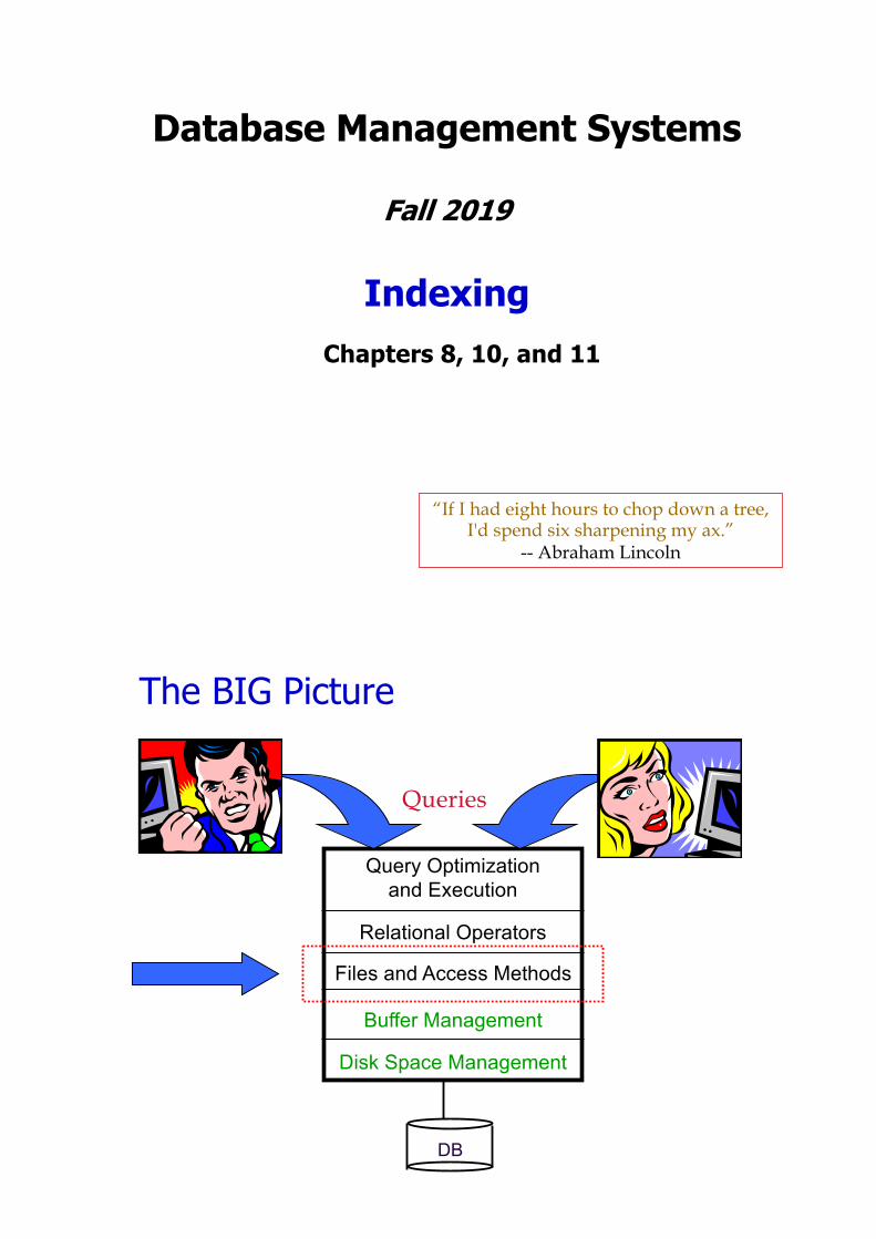
The BIG Picture

Query Optimizationand Execution

Relational Operators

Files and Access Methods

Buffer Management

Disk Space Management

DB

Queries

DBMS vs. OS File SystemOS does disk space & buffer mgmt: why not let OS manage these tasks?

• Some limitations, e.g., files can’t span disks.

§ Note, this is changing --- OS File systems are getting smarter (i.e., more like databases!)

• Buffer management in DBMS requires ability to:

§ pin a page in buffer pool, force a page to disk & order writes (important for implementing CC & recovery)

§ adjust replacement policy, and pre-fetch pages based on access patterns in typical DB operations.

• Q: Compare DBMS Buffer Mgmt to OS Virtual Memory? to Processor Cache?

Files of Records• Blocks interface for I/O, but…

• Higher levels of DBMS operate on records, and

files of records.

• FILE: A collection of pages, each containing a

collection of records. Must support:

insert/delete/modify recordfetch a particular record (specified using record id)scan all records (possibly with some conditions on

the records to be retrieved)

• Note: typically

page size = block size = frame size.

Data Dictionary Storage

• The Data dictionary (also called system catalog) stores metadata; that is, data about data, such as:

• Information about relations

§ names of relations§ names, types and lengths of attributes of each relation§ names and definitions of views§ integrity constraints

• User and accounting information, including passwords

• Statistical and descriptive data

§ number of tuples in each relation • Physical file organization information

§ How relation is stored (sequential/hash/...)§ Physical location of relation

“MetaData” - System Catalogs• How to impose structure on all those bytes??

• MetaData: “Data about Data”

• For each relation:§ name, file location, file structure (e.g., Heap file)§ attribute name and type, for each attribute§ index name, for each index§ integrity constraints

• For each index:

§ structure (e.g., B+ tree) and search key fields• For each view:

§ view name and definition• Plus statistics, authorization, buffer pool size,

etc.

! Q: But how to store the catalogs????

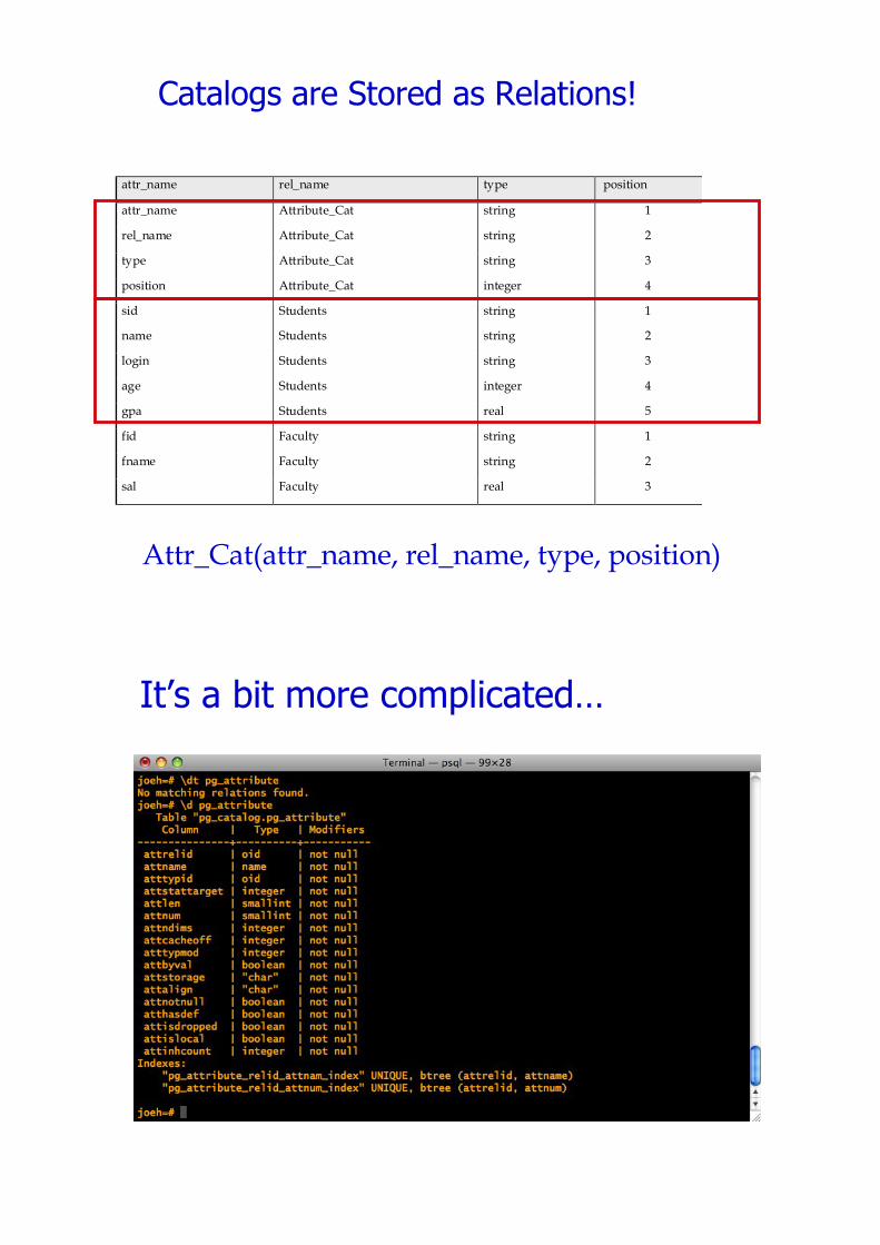
Catalogs are Stored as Relations!

attr_name rel_name type position

attr_name Attribute_Cat string 1

rel_name Attribute_Cat string 2

type Attribute_Cat string 3

position Attribute_Cat integer 4

sid Students string 1

name Students string 2

login Students string 3

age Students integer 4

gpa Students real 5

fid Faculty string 1

fname Faculty string 2

sal Faculty real 3

Attr_Cat(attr_name, rel_name, type, position)

It’s a bit more complicated…

File Organization

• The database is stored as a collection of files.

Each file is a sequence of records. A record is a

sequence of fields.

• One approach:

§ Assume record size is fixed§ Each file has records of one particular type only§ Different files are used for different relations

• This case is easiest to implement; will consider

variable length records later.

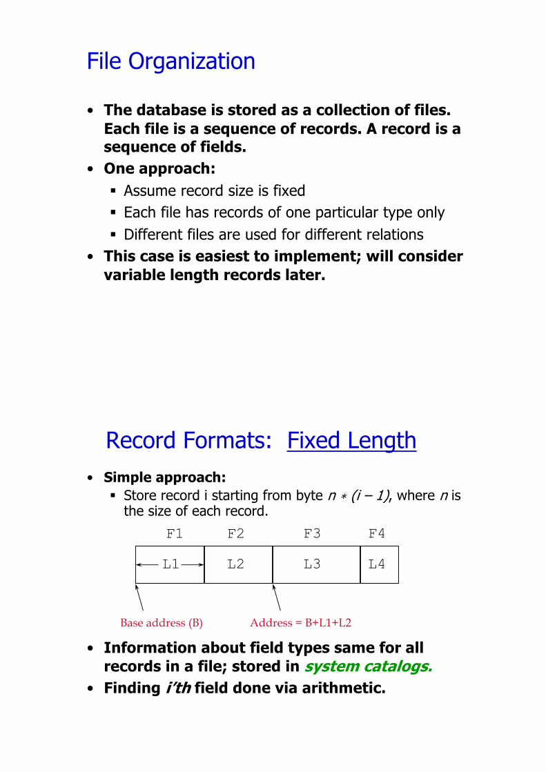
Record Formats: Fixed Length

• Information about field types same for all

records in a file; stored in system catalogs.

• Finding i’th field done via arithmetic.

Base address (B)

L1 L2 L3 L4

F1 F2 F3 F4

Address = B+L1+L2

• Simple approach:

§ Store record i starting from byte n ∗ (i – 1), where n is the size of each record.

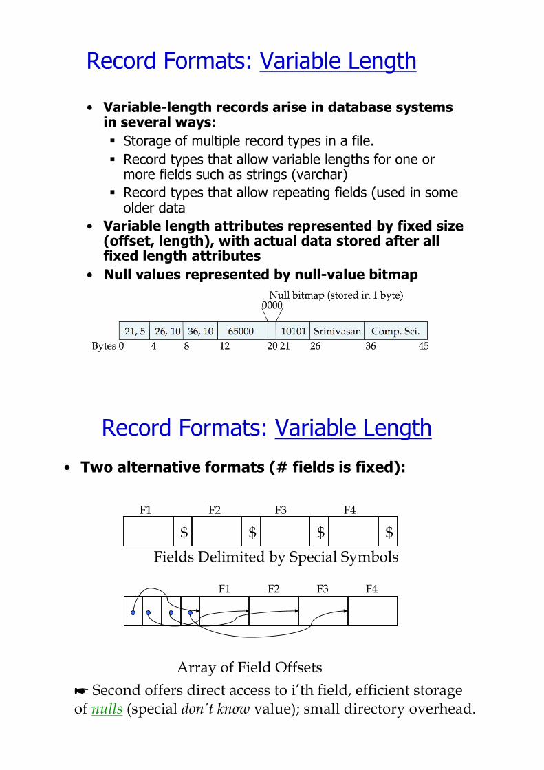
Record Formats: Variable Length

• Variable-length records arise in database systems in several ways:

§ Storage of multiple record types in a file. § Record types that allow variable lengths for one or

more fields such as strings (varchar) § Record types that allow repeating fields (used in some

older data • Variable length attributes represented by fixed size

(offset, length), with actual data stored after all fixed length attributes

• Null values represented by null-value bitmap

Record Formats: Variable Length• Two alternative formats (# fields is fixed):

! Second offers direct access to i’th field, efficient storage of nulls (special don’t know value); small directory overhead.

$ $ $ $Fields Delimited by Special Symbols

F1 F2 F3 F4

F1 F2 F3 F4

Array of Field Offsets

How to Identify a Record?• The Relational Model doesn’t expose

“pointers”, but that doesn’t mean that the

DBMS doesn’t use them internally.

• Q: Can we use memory addresses to “point” to

records?

• Systems use a “Record ID” or “RecID”

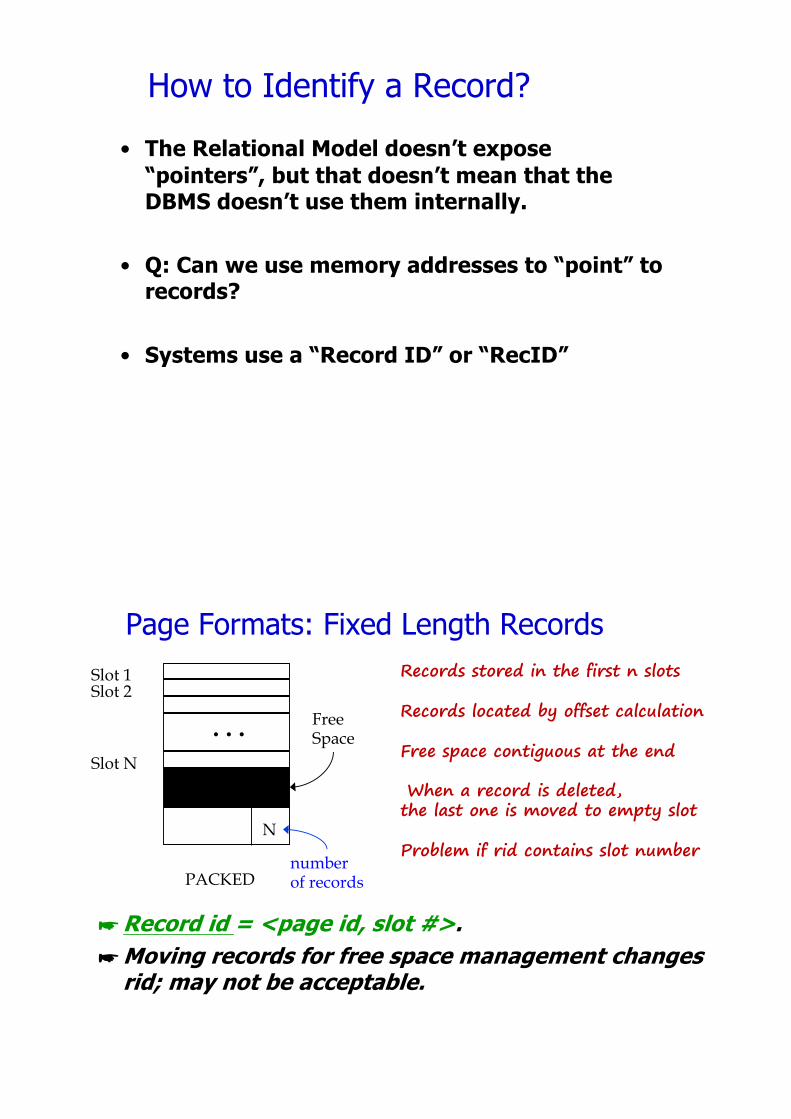
Page Formats: Fixed Length Records

!Record id = <page id, slot #>.

!Moving records for free space management changes rid; may not be acceptable.

Slot 1Slot 2

Slot N

. . .

N

PACKED

FreeSpace

number of records

Records stored in the first n slots

Records located by offset calculation

Free space contiguous at the end

When a record is deleted, the last one is moved to empty slot

Problem if rid contains slot number

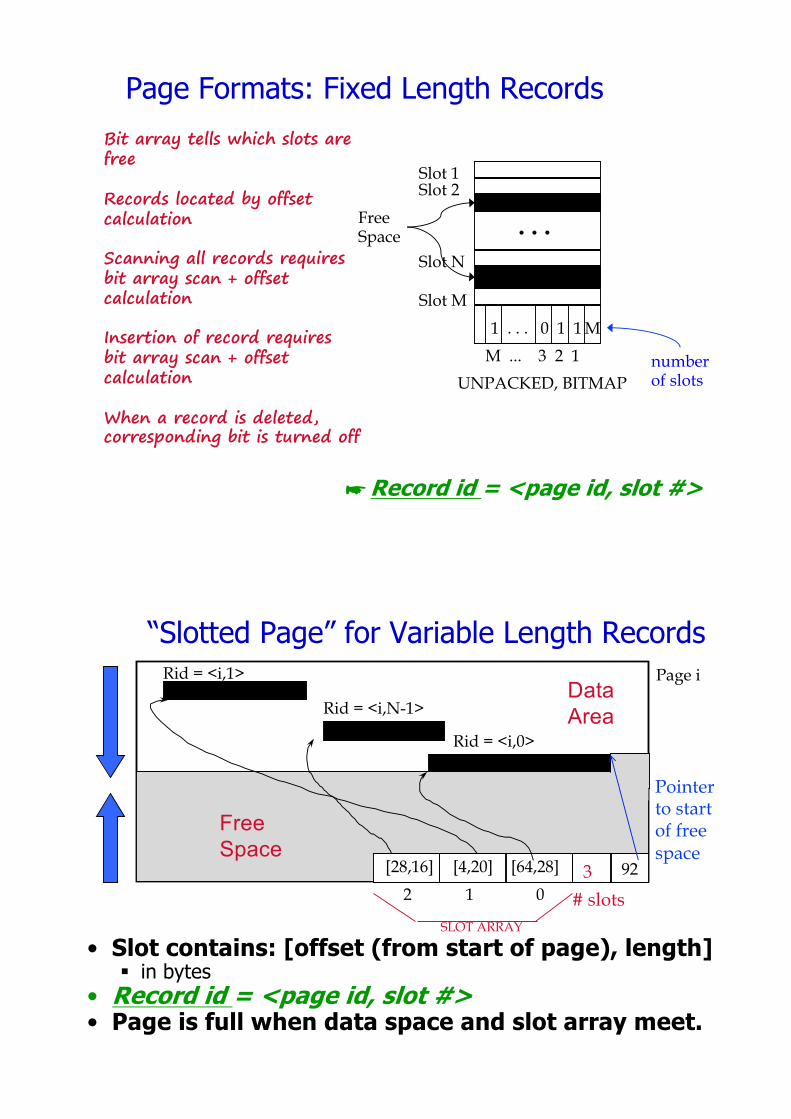
Page Formats: Fixed Length Records

!Record id = <page id, slot #>

. . .

M10. . .M ... 3 2 1

UNPACKED, BITMAP

Slot 1Slot 2

Slot N

FreeSpace

Slot M11

numberof slots

Bit array tells which slots are free

Records located by offset calculation

Scanning all records requiresbit array scan + offset calculation

Insertion of record requiresbit array scan + offset calculation

When a record is deleted, corresponding bit is turned off

“Slotted Page” for Variable Length Records

• Slot contains: [offset (from start of page), length]§ in bytes

• Record id = <page id, slot #>• Page is full when data space and slot array meet.

Page iRid = <i,1>

Rid = <i,N-1>

Rid = <i,0>

Pointerto startof freespace

SLOT ARRAY

2 1 03

# slots

DataArea

Free Space

[4,20][28,16] [64,28] 92

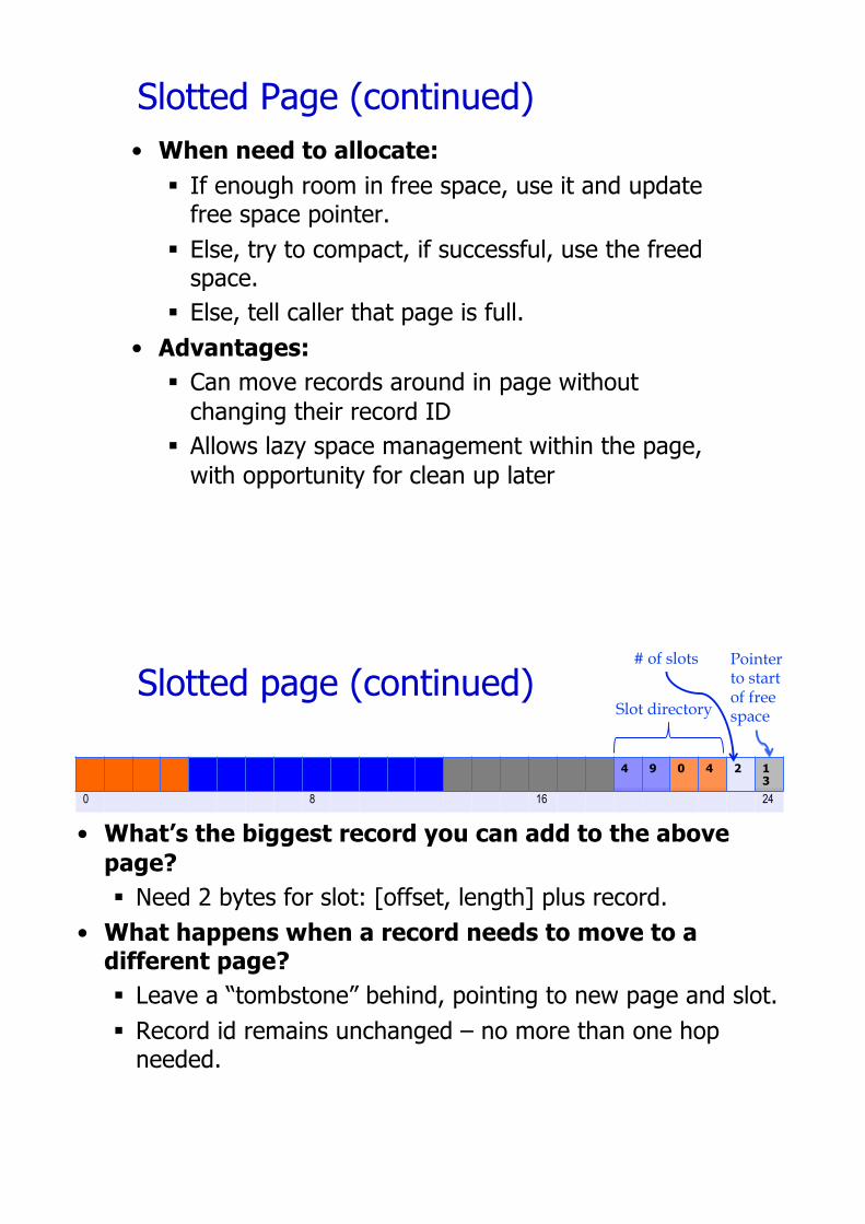
Slotted Page (continued)• When need to allocate:

§ If enough room in free space, use it and update free space pointer.

§ Else, try to compact, if successful, use the freed space.

§ Else, tell caller that page is full.• Advantages:

§ Can move records around in page without changing their record ID

§ Allows lazy space management within the page, with opportunity for clean up later

0 8 16 24

Slotted page (continued)

• What’s the biggest record you can add to the above

page?

§ Need 2 bytes for slot: [offset, length] plus record.• What happens when a record needs to move to a

different page?

§ Leave a “tombstone” behind, pointing to new page and slot.§ Record id remains unchanged – no more than one hop

needed.

4 9 0 4 2 13

Pointerto startof freespaceSlot directory

# of slots

So far we’ve organized:

• Fields into Records (fixed and variable length)

• Records into Pages (fixed and variable length)

Now we need to organize Pages into Files

Alternative File OrganizationsMany alternatives exist, each good for some

situations, and not so good in others:

Heap files: Unordered. Suitable when typical access is a file scan retrieving all records. Easy to maintain.

Sorted Files: Best for retrieval in search key order, or if only a `range’ of records is needed. Expensive to maintain.

Clustered Files (with Indexes): A compromise between the above two extremes.

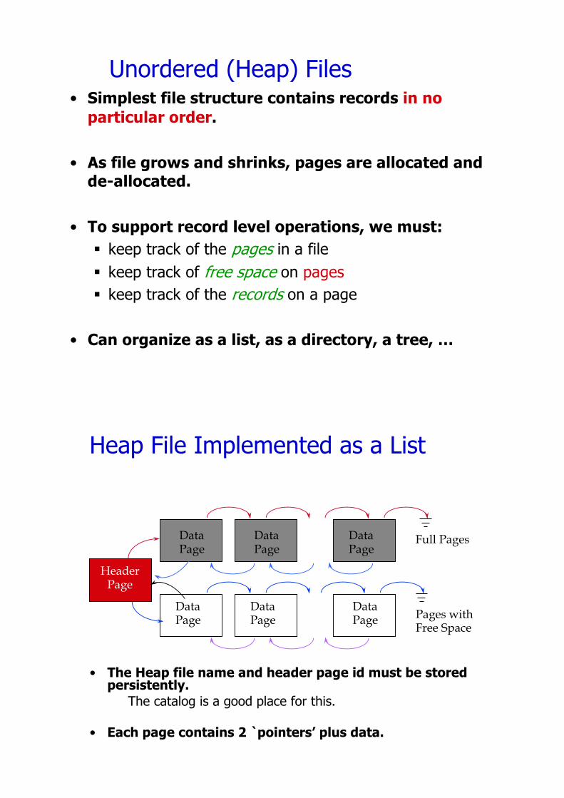
Unordered (Heap) Files• Simplest file structure contains records in no

particular order.

• As file grows and shrinks, pages are allocated and

de-allocated.

• To support record level operations, we must:

§ keep track of the pages in a file§ keep track of free space on pages§ keep track of the records on a page

• Can organize as a list, as a directory, a tree, …

Heap File Implemented as a List

• The Heap file name and header page id must be stored persistently.

The catalog is a good place for this.

• Each page contains 2 `pointers’ plus data.

HeaderPage

DataPage

DataPage

DataPage

DataPage

DataPage

DataPage Pages with

Free Space

Full Pages

Cost Model for AnalysisWe ignore CPU costs, for simplicity:

§ B: The number of data blocks§ R: Number of records per block§ D: (Average) time to read or write disk block

• Measuring number of block I/O’s ignores gains of pre-fetching and sequential access; thus, even I/O cost is only loosely approximated.

• Average-case analysis; based on several simplistic assumptions.§ Often called a “back of the envelope” calculation.

! Good enough to show the overall trends!

Some Assumptions in the Analysis

• Single record insert and delete.

• Equality selection - exactly one match (what if

more or less???).

• For Heap Files we’ll assume:

§ Insert always appends to end of file.§ Delete just leaves free space in the page.§ Empty pages are not deallocated.

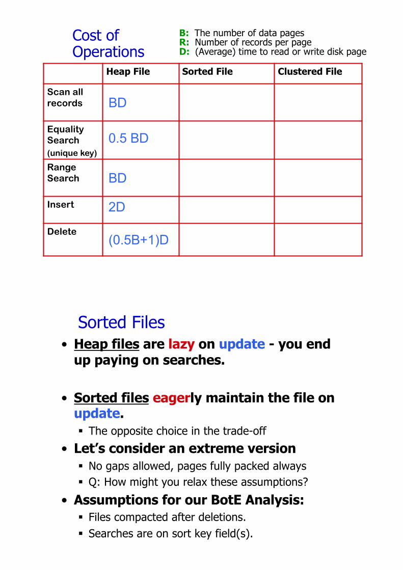
Cost of Operations

Heap File Sorted File Clustered File

Scan all records

Equality Search(unique key)

Range Search

Insert

Delete

B: The number of data pagesR: Number of records per pageD: (Average) time to read or write disk page

BD

0.5 BD

BD

2D

(0.5B+1)D

Sorted Files• Heap files are lazy on update - you end

up paying on searches.

• Sorted files eagerly maintain the file on update.

§ The opposite choice in the trade-off• Let’s consider an extreme version

§ No gaps allowed, pages fully packed always§ Q: How might you relax these assumptions?

• Assumptions for our BotE Analysis:

§ Files compacted after deletions.§ Searches are on sort key field(s).

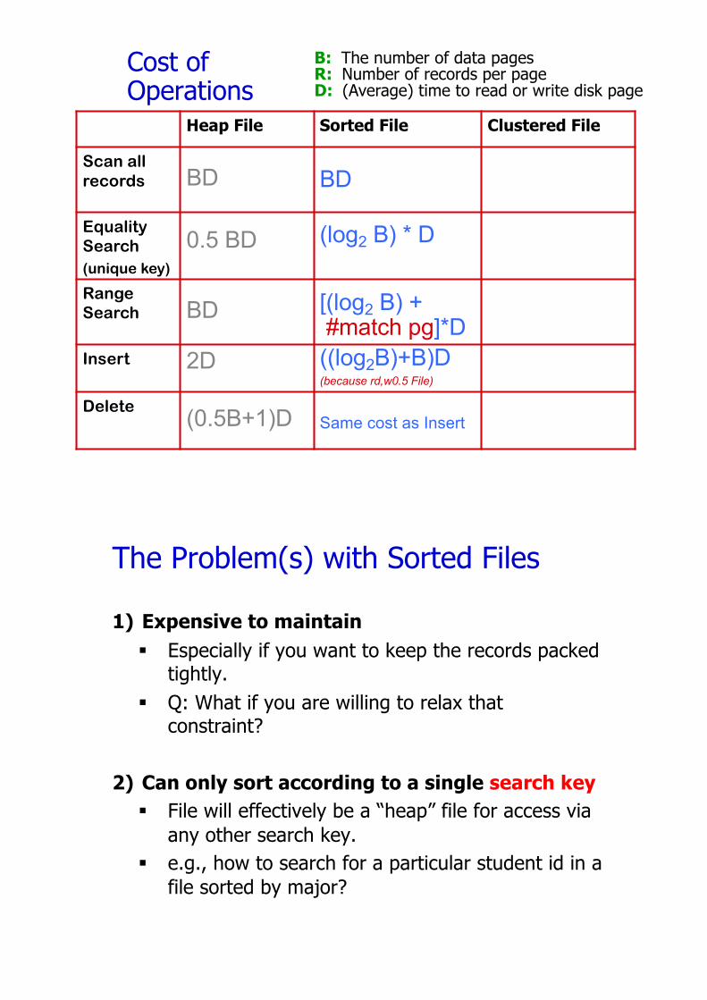
Cost of Operations

Heap File Sorted File Clustered File

Scan all records

Equality Search(unique key)

Range Search

Insert

Delete

B: The number of data pagesR: Number of records per pageD: (Average) time to read or write disk page

BD

(log2 B) * D

[(log2 B) +#match pg]*D((log2B)+B)D(because rd,w0.5 File)

Same cost as Insert

BD

0.5 BD

BD

2D

(0.5B+1)D

The Problem(s) with Sorted Files

1) Expensive to maintain

§ Especially if you want to keep the records packed tightly.

§ Q: What if you are willing to relax that constraint?

2) Can only sort according to a single search key

§ File will effectively be a “heap” file for access via any other search key.

§ e.g., how to search for a particular student id in a file sorted by major?

Indexes: Introduction

• Sometimes, we want to retrieve records by specifying values in one or more fields, e.g.,

§ Find all students in the “CS” department§ Find all students with a gpa > 3.0§ Find all students in CS with a gpa > 3.0

• An index on a file is a disk-based data structure that speeds up selections on some search key fields.

§ Any subset of the fields of a relation can be the search key for an index on the relation.

§ Search key is not the same as key§ e.g., Search key doesn’t have to be unique.

Indexes: Overview

• An index contains a collection of data entries,

and supports efficient retrieval of all records

with a given search key value k.

§ Typically, index also contains auxiliary information that directs searches to the desired data entries

• Many indexing techniques exist:

§ B+ trees, hash-based structures, R trees, …

• Can have multiple (different) indexes per file.

§ E.g. file sorted by age, with a hash index on salaryand a B+tree index on name.

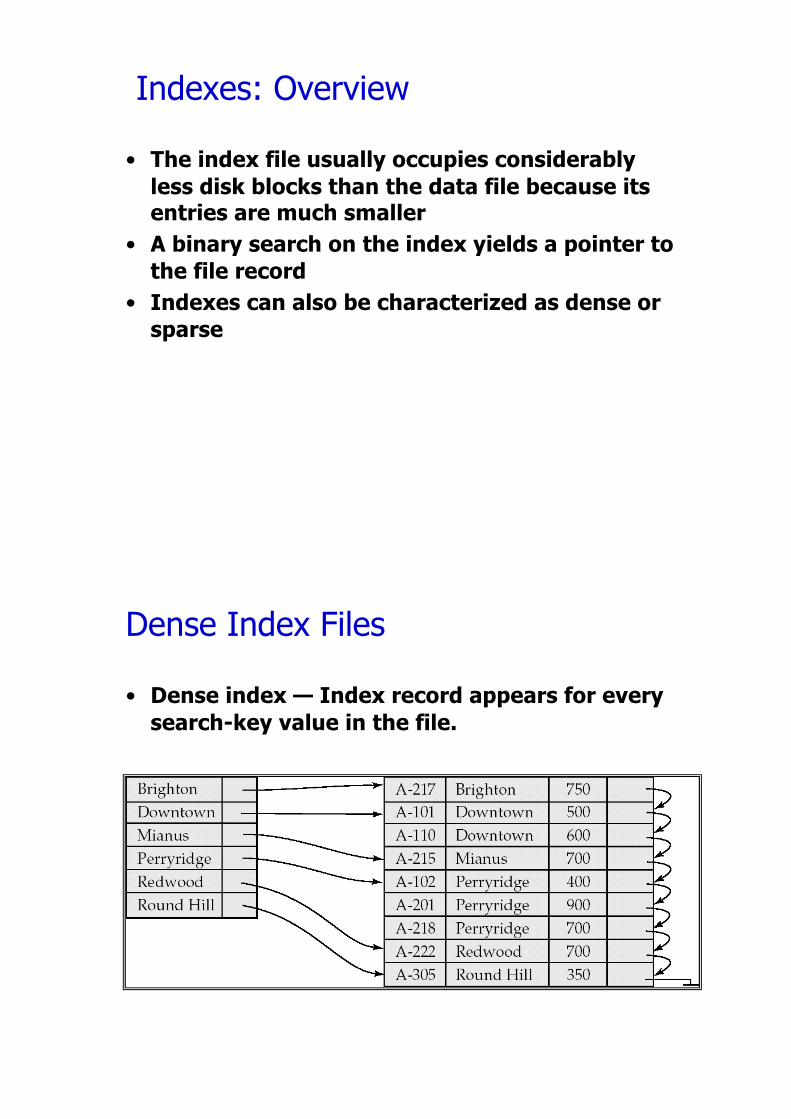
Indexes: Overview

• The index file usually occupies considerably

less disk blocks than the data file because its

entries are much smaller

• A binary search on the index yields a pointer to

the file record

• Indexes can also be characterized as dense or

sparse

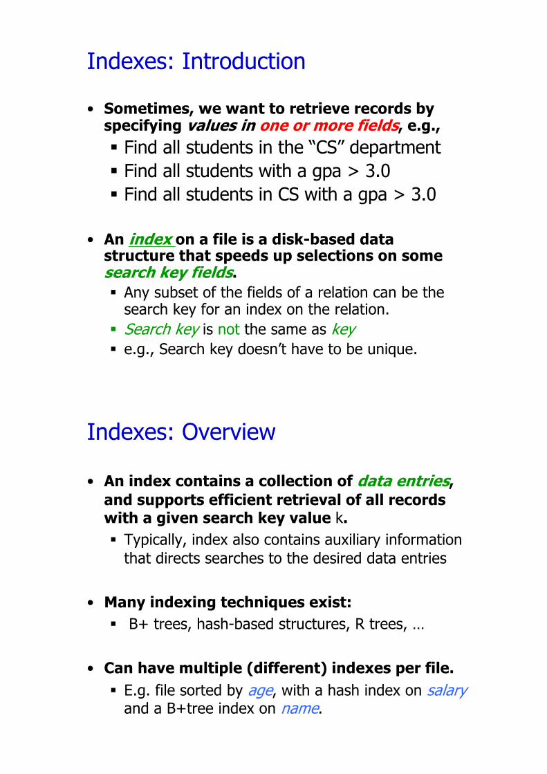
Dense Index Files

• Dense index — Index record appears for every

search-key value in the file.

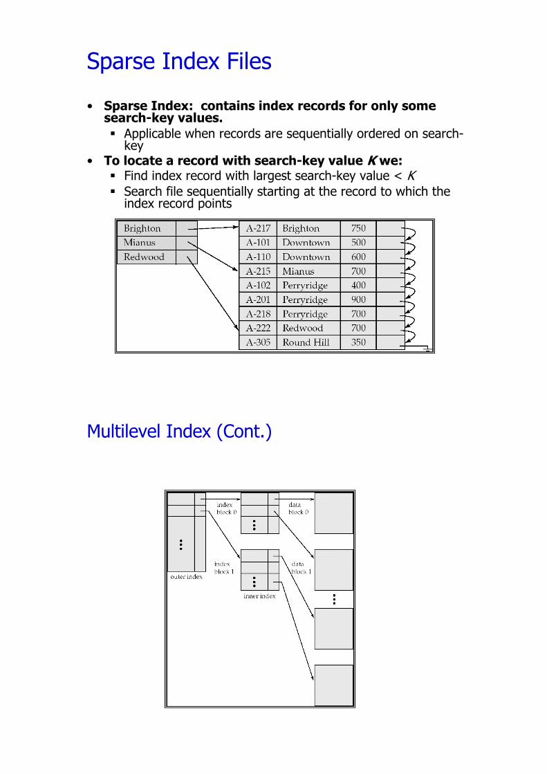
Sparse Index Files• Sparse Index: contains index records for only some

search-key values.

§ Applicable when records are sequentially ordered on search-key

• To locate a record with search-key value K we:§ Find index record with largest search-key value < K§ Search file sequentially starting at the record to which the

index record points

Multilevel Index (Cont.)

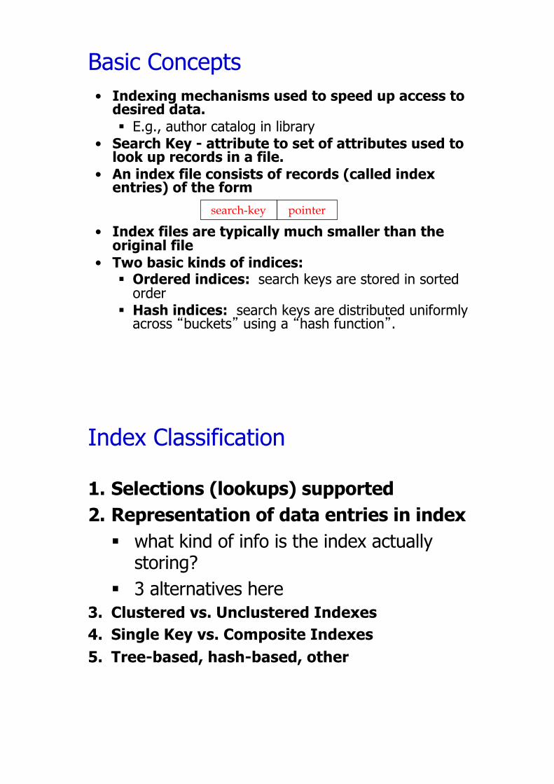
Basic Concepts• Indexing mechanisms used to speed up access to

desired data.

§ E.g., author catalog in library• Search Key - attribute to set of attributes used to

look up records in a file.

• An index file consists of records (called index entries) of the form

• Index files are typically much smaller than the original file

• Two basic kinds of indices:§ Ordered indices: search keys are stored in sorted

order§ Hash indices: search keys are distributed uniformly

across “buckets” using a “hash function”.

search-key pointer

Index Classification

1. Selections (lookups) supported

2. Representation of data entries in index

§ what kind of info is the index actually storing?

§ 3 alternatives here3. Clustered vs. Unclustered Indexes

4. Single Key vs. Composite Indexes

5. Tree-based, hash-based, other

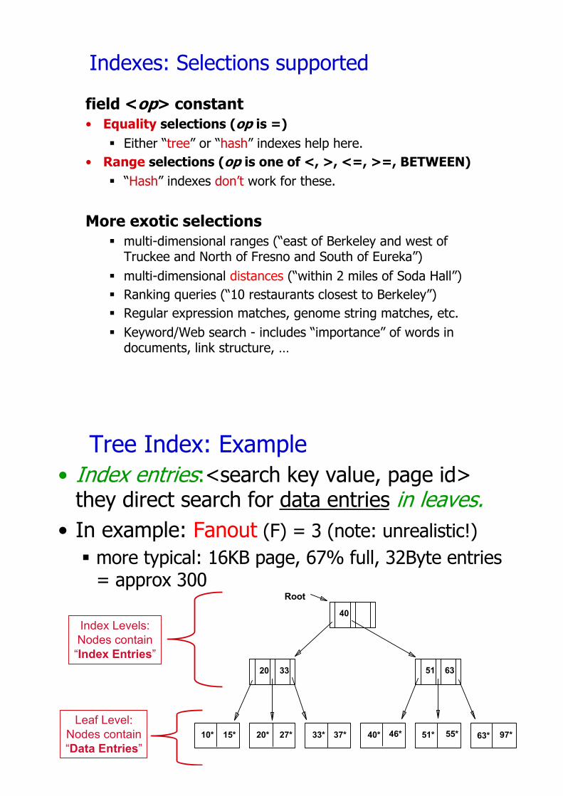
Indexes: Selections supported

field <op> constant

• Equality selections (op is =)

§ Either “tree” or “hash” indexes help here.• Range selections (op is one of <, >, <=, >=, BETWEEN)

§ “Hash” indexes don’t work for these.

More exotic selections

§ multi-dimensional ranges (“east of Berkeley and west of Truckee and North of Fresno and South of Eureka”)

§ multi-dimensional distances (“within 2 miles of Soda Hall”)§ Ranking queries (“10 restaurants closest to Berkeley”)§ Regular expression matches, genome string matches, etc.§ Keyword/Web search - includes “importance” of words in

documents, link structure, …

Tree Index: Example• Index entries:<search key value, page id>

they direct search for data entries in leaves.• In example: Fanout (F) = 3 (note: unrealistic!)

§ more typical: 16KB page, 67% full, 32Byte entries = approx 300

10* 15* 20* 27* 33* 37* 40* 46* 51* 55* 63* 97*

20 33 51 63

40

Root

Leaf Level:Nodes contain“Data Entries”

Index Levels:Nodes contain

“Index Entries”

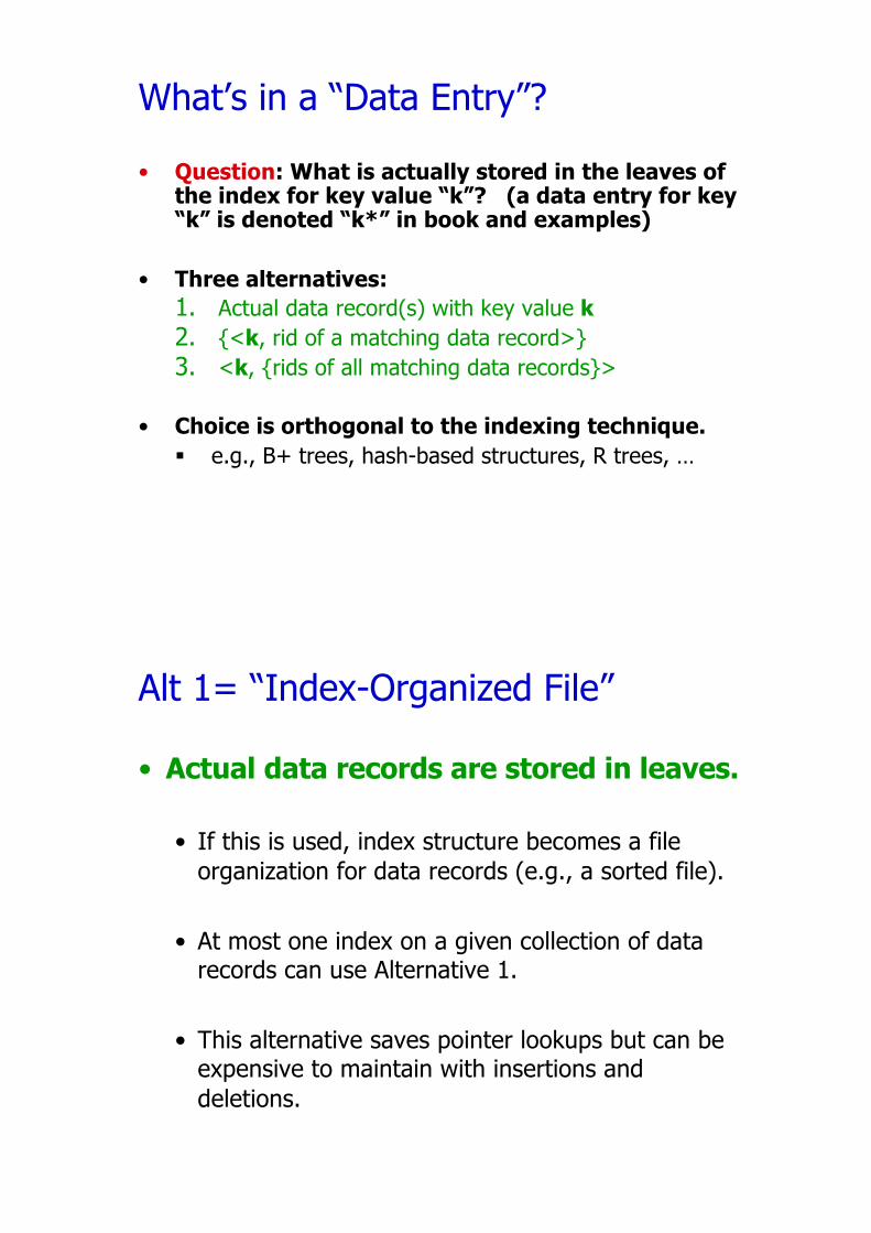
What’s in a “Data Entry”?

• Question: What is actually stored in the leaves of the index for key value “k”? (a data entry for key “k” is denoted “k*” in book and examples)

• Three alternatives:

1. Actual data record(s) with key value k

2. {<k, rid of a matching data record>}3. <k, {rids of all matching data records}>

• Choice is orthogonal to the indexing technique.

§ e.g., B+ trees, hash-based structures, R trees, …

Alt 1= “Index-Organized File”

• Actual data records are stored in leaves.

• If this is used, index structure becomes a file organization for data records (e.g., a sorted file).

• At most one index on a given collection of data records can use Alternative 1.

• This alternative saves pointer lookups but can be expensive to maintain with insertions and deletions.

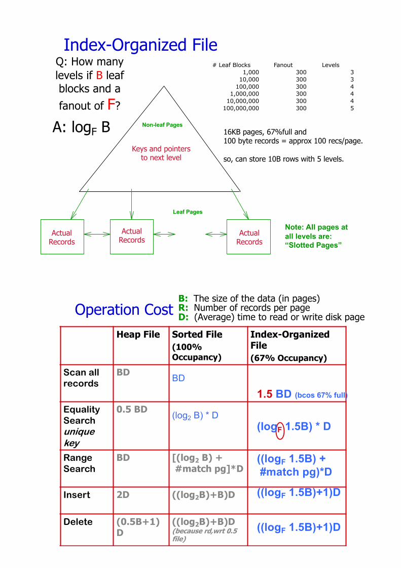
Index-Organized File

Leaf Pages

Non-leaf Pages

Keys and pointers to next level

Actual Records

Actual Records

Actual Records

Q: How many levels if B leaf blocks and a fanout of F?

A: logF B

# Leaf Blocks Fanout Levels1,000 300 3

10,000 300 3100,000 300 4

1,000,000 300 410,000,000 300 4

100,000,000 300 5

16KB pages, 67%full and 100 byte records = approx 100 recs/page.

so, can store 10B rows with 5 levels.

Note: All pages at

all levels are:

“Slotted Pages”

Operation CostHeap File Sorted File

(100%

Occupancy)

Index-Organized File

(67% Occupancy)

Scan all records

BD BD

Equality Search unique key

0.5 BD(log2 B) * D

Range Search

BD [(log2 B) +

#match pg]*D

Insert 2D ((log2B)+B)D

Delete (0.5B+1) D

((log2B)+B)D (because rd,wrt 0.5 file)

B: The size of the data (in pages)R: Number of records per pageD: (Average) time to read or write disk page

1.5 BD (bcos 67% full)

(logF 1.5B) * D

((logF 1.5B) +

#match pg)*D

((logF 1.5B)+1)D

((logF 1.5B)+1)D

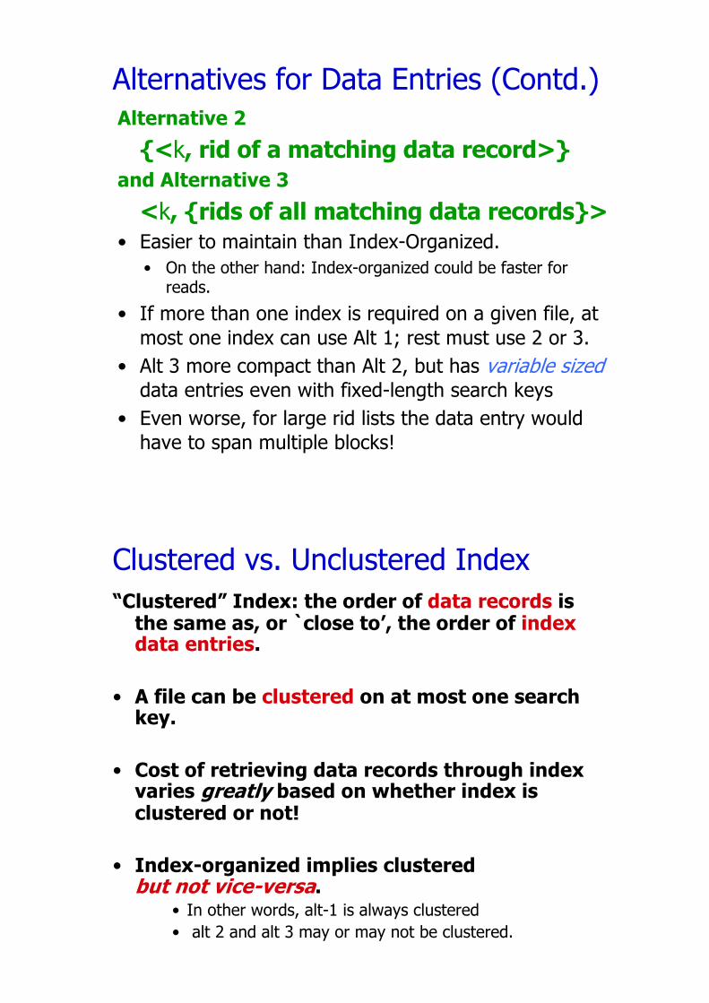
Alternatives for Data Entries (Contd.)Alternative 2

{<k, rid of a matching data record>}

and Alternative 3

<k, {rids of all matching data records}>

• Easier to maintain than Index-Organized.• On the other hand: Index-organized could be faster for

reads.• If more than one index is required on a given file, at

most one index can use Alt 1; rest must use 2 or 3.• Alt 3 more compact than Alt 2, but has variable sized

data entries even with fixed-length search keys • Even worse, for large rid lists the data entry would

have to span multiple blocks!

Clustered vs. Unclustered Index“Clustered” Index: the order of data records is

the same as, or `close to’, the order of index data entries.

• A file can be clustered on at most one search key.

• Cost of retrieving data records through index varies greatly based on whether index is clustered or not!

• Index-organized implies clustered but not vice-versa.

• In other words, alt-1 is always clustered• alt 2 and alt 3 may or may not be clustered.

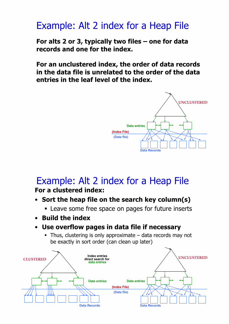
Example: Alt 2 index for a Heap File

Index entries

Data entries

direct search for

(Index File)

(Data file)

Data Records

data entries

Data entries

Data Records

CLUSTERED UNCLUSTERED

For alts 2 or 3, typically two files – one for data

records and one for the index.

For an unclustered index, the order of data records

in the data file is unrelated to the order of the data

entries in the leaf level of the index.

Example: Alt 2 index for a Heap FileFor a clustered index:

• Sort the heap file on the search key column(s)

§ Leave some free space on pages for future inserts• Build the index

• Use overflow pages in data file if necessary

§ Thus, clustering is only approximate – data records may not be exactly in sort order (can clean up later)

Index entries

Data entries

direct search for

(Index File)

(Data file)

Data Records

data entries

Data entries

Data Records

CLUSTERED UNCLUSTERED

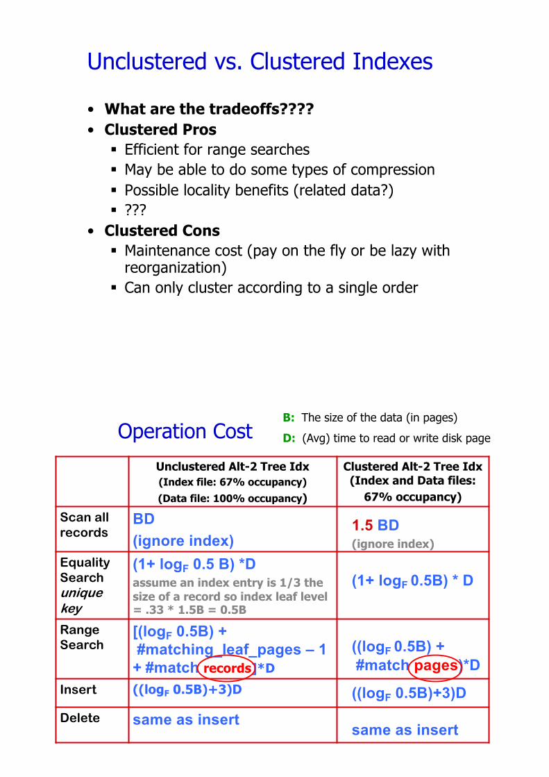
Unclustered vs. Clustered Indexes

• What are the tradeoffs????

• Clustered Pros

§ Efficient for range searches§ May be able to do some types of compression§ Possible locality benefits (related data?)§ ???

• Clustered Cons

§ Maintenance cost (pay on the fly or be lazy with reorganization)

§ Can only cluster according to a single order

Operation CostUnclustered Alt-2 Tree Idx

(Index file: 67% occupancy)

(Data file: 100% occupancy)

Clustered Alt-2 Tree Idx

(Index and Data files:

67% occupancy)

Scan all records

BD

(ignore index)

Equality Search unique key

(1+ logF 0.5 B) *D

assume an index entry is 1/3 the

size of a record so index leaf level = .33 * 1.5B = 0.5B

Range Search

[(logF 0.5B) +

#matching_leaf_pages – 1

+ #match records]*D

Insert ((logF 0.5B)+3)D

Delete same as insert

B: The size of the data (in pages)D: (Avg) time to read or write disk page

1.5 BD

(ignore index)

(1+ logF 0.5B) * D

((logF 0.5B) +

#match pages)*D

((logF 0.5B)+3)D

same as insert

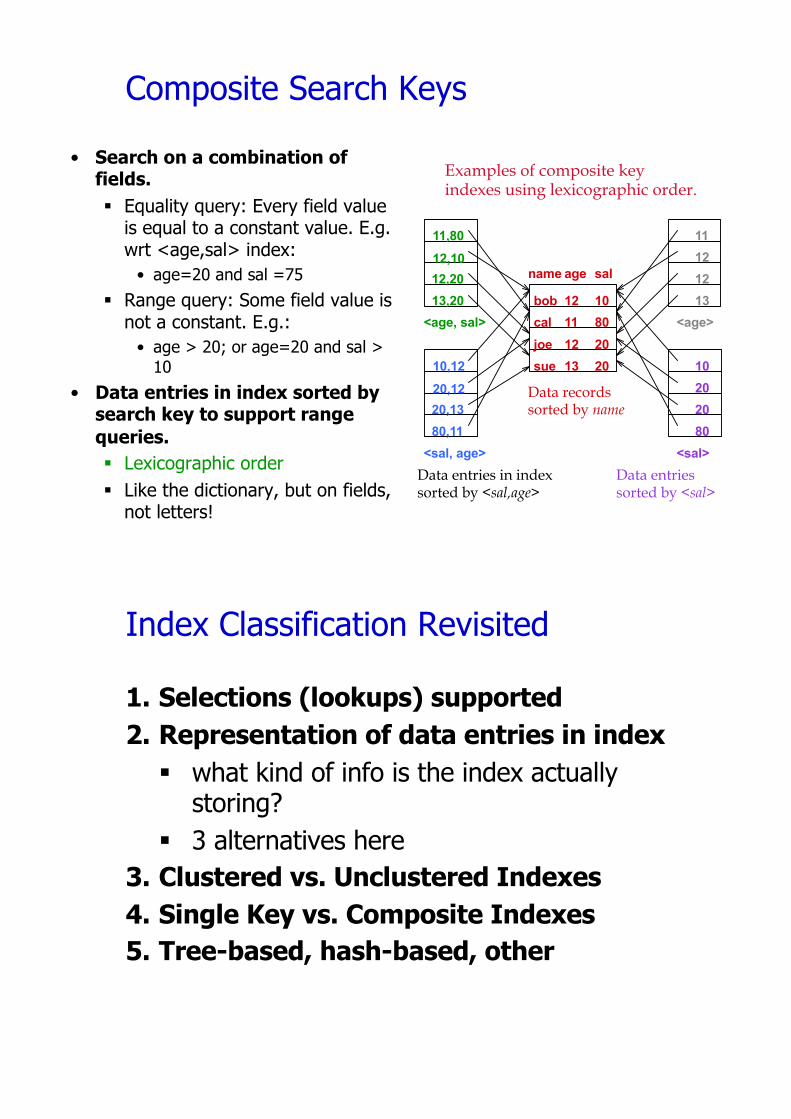
Composite Search Keys

• Search on a combination of fields.

§ Equality query: Every field value is equal to a constant value. E.g. wrt <age,sal> index:

• age=20 and sal =75§ Range query: Some field value is

not a constant. E.g.:• age > 20; or age=20 and sal >

10• Data entries in index sorted by

search key to support range

queries.

§ Lexicographic order § Like the dictionary, but on fields,

not letters!

sue 13 20

bob

cal

joe 12

10

20

8011

12

name age sal

<sal, age>

<age, sal> <age>

<sal>

12,20

12,10

11,80

13,20

20,12

10,12

20,13

80,11

11

12

12

13

10

20

20

80

Data recordssorted by name

Data entries in indexsorted by <sal,age>

Data entriessorted by <sal>

Examples of composite keyindexes using lexicographic order.

Index Classification Revisited

1. Selections (lookups) supported

2. Representation of data entries in index

§ what kind of info is the index actually storing?

§ 3 alternatives here3. Clustered vs. Unclustered Indexes

4. Single Key vs. Composite Indexes

5. Tree-based, hash-based, other

Tree-Structured Indexes

• Tree-structured indexing techniques support

both range searches and equality searches.

• Two examples:

§ ISAM: static structure; early index technology.

§ B+ tree: dynamic, adjusts gracefully under inserts and deletes.

ISAM = Indexed Sequential AccessMethod• ISAM is an old-fashioned idea

§ B+ trees are usually better, as we’ll see• Though not always

• But, it’s a good place to start

§ Simpler than B+ tree, but many of the same ideas

• Upshot

§ Don’t brag about being an ISAM expert on your resume

§ Do understand how they work, and tradeoffs with B+ trees

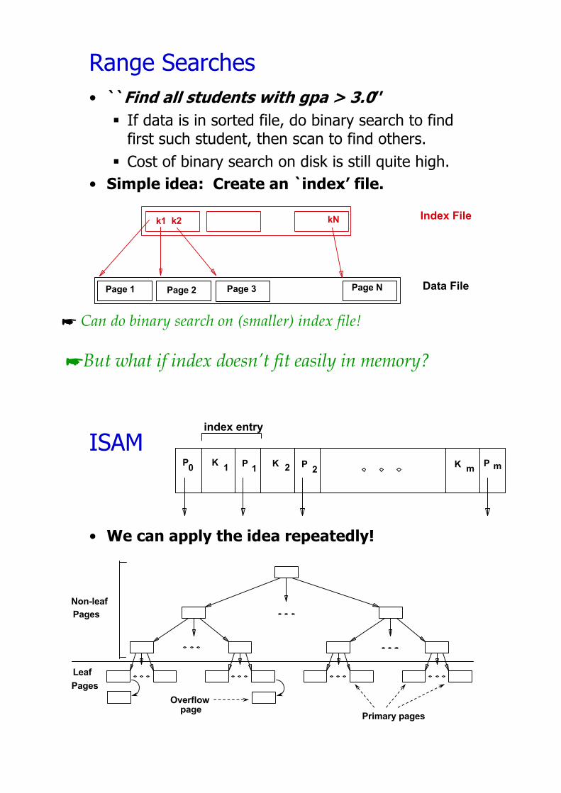
Range Searches• ``Find all students with gpa > 3.0’’

§ If data is in sorted file, do binary search to find first such student, then scan to find others.

§ Cost of binary search on disk is still quite high. • Simple idea: Create an `index’ file.

! Can do binary search on (smaller) index file!

Page 1 Page 2 Page NPage 3 Data File

k2 kNk1Index File

!But what if index doesn’t fit easily in memory?

ISAM

• We can apply the idea repeatedly!

P0

K1

P1

K2 P

2K

mP m

index entry

Non-leaf

Pages

Pages

Overflow page

Primary pages

Leaf

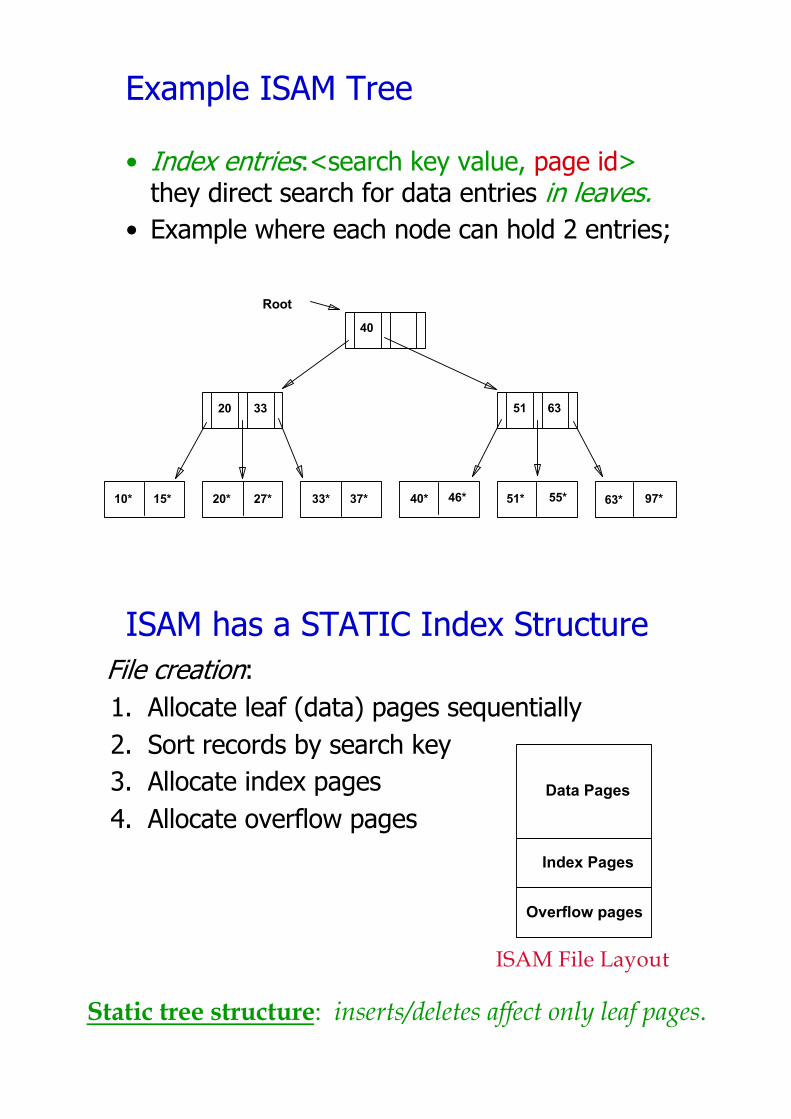
Example ISAM Tree

• Index entries:<search key value, page id>they direct search for data entries in leaves.

• Example where each node can hold 2 entries;

10* 15* 20* 27* 33* 37* 40* 46* 51* 55* 63* 97*

20 33 51 63

40

Root

Data Pages

ISAM has a STATIC Index StructureFile creation: 1. Allocate leaf (data) pages sequentially2. Sort records by search key 3. Allocate index pages4. Allocate overflow pages

Static tree structure: inserts/deletes affect only leaf pages.

ISAM File Layout

Index Pages

Overflow pages

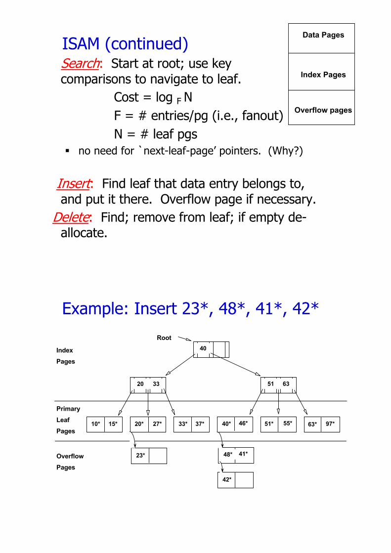
ISAM (continued)Search: Start at root; use key comparisons to navigate to leaf.

Cost = log F N F = # entries/pg (i.e., fanout)N = # leaf pgs

§ no need for `next-leaf-page’ pointers. (Why?)

Insert: Find leaf that data entry belongs to, and put it there. Overflow page if necessary.

Delete: Find; remove from leaf; if empty de-allocate.

Data Pages

Index Pages

Overflow pages

Example: Insert 23*, 48*, 41*, 42*

48*

10* 15* 20* 27* 33* 37* 40* 46* 51* 55* 63* 97*

20 33 51 63

40

Root

Overflow

Pages

Leaf

Index

Pages

Pages

Primary

23* 41*

42*

48*

10* 15* 20* 27* 33* 37* 40* 46* 51* 55* 63* 97*

20 33 51 63

40

Root

Overflow

Pages

Leaf

Index

Pages

Pages

Primary

23* 41*

42*

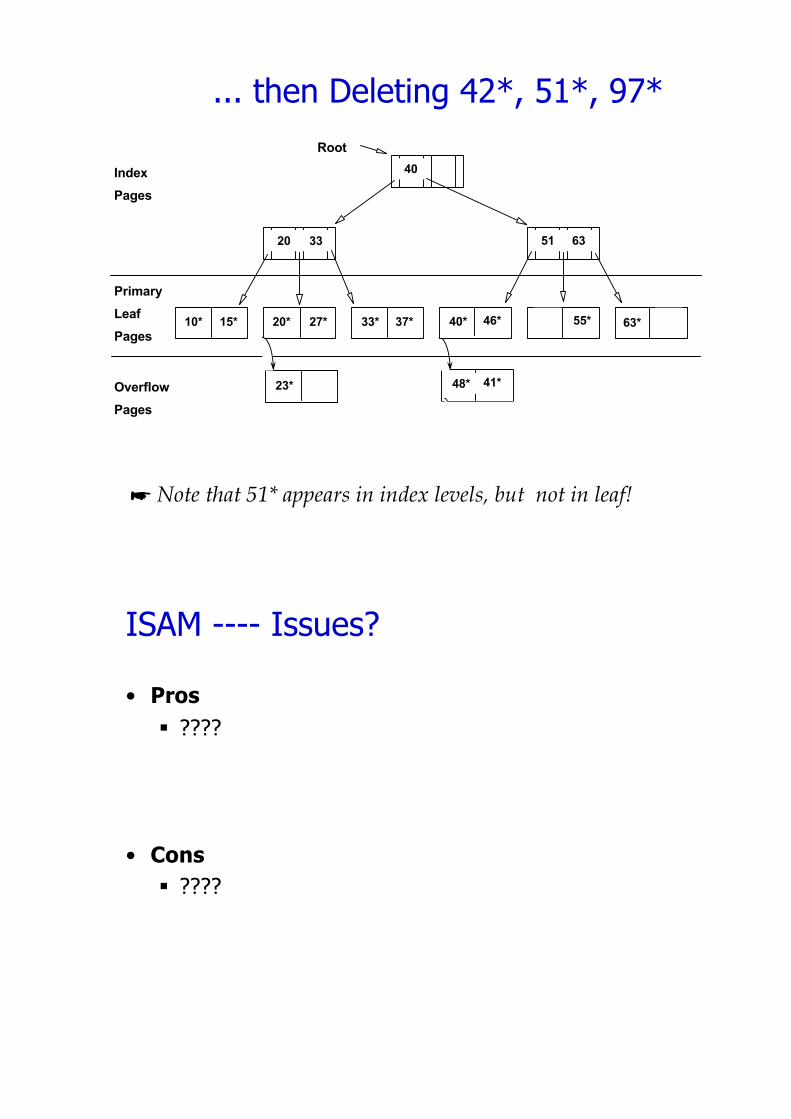
... then Deleting 42*, 51*, 97*

! Note that 51* appears in index levels, but not in leaf!

ISAM ---- Issues?

• Pros

§ ????

• Cons

§ ????

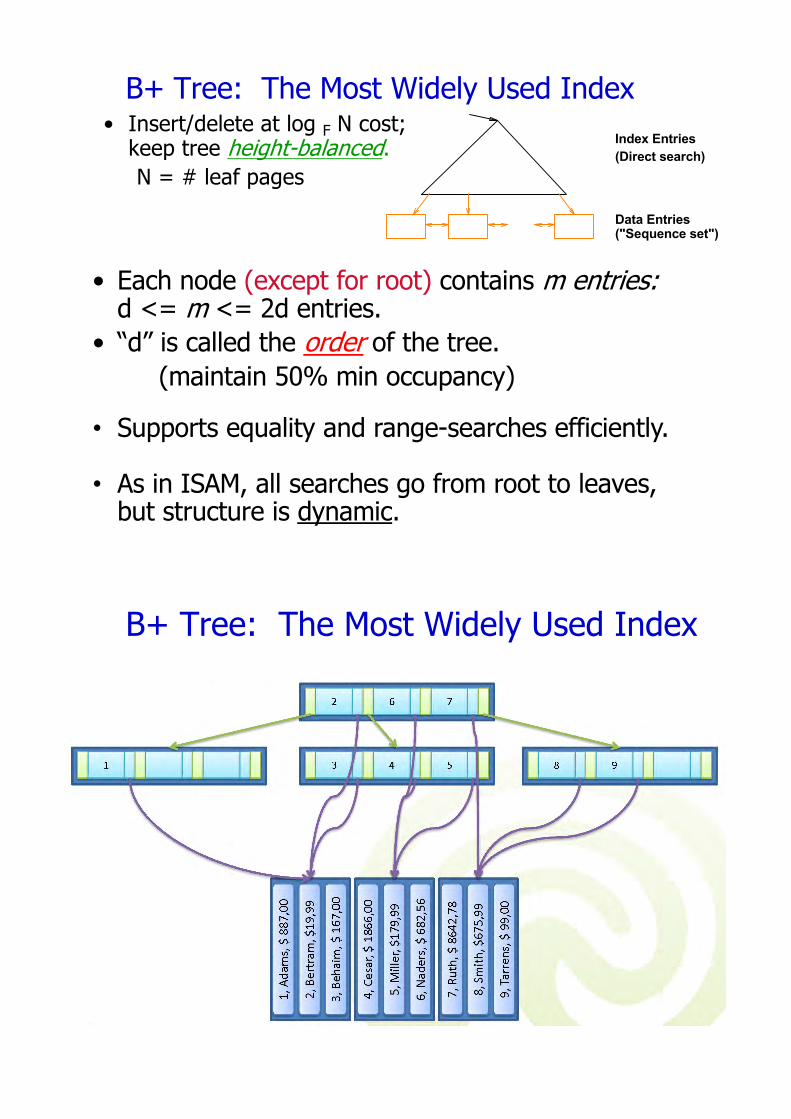
B+ Tree: The Most Widely Used Index• Insert/delete at log F N cost;

keep tree height-balanced. N = # leaf pages

Index Entries

Data Entries

("Sequence set")

(Direct search)

• Each node (except for root) contains m entries:d <= m <= 2d entries.

• “d” is called the order of the tree. (maintain 50% min occupancy)

• Supports equality and range-searches efficiently.

• As in ISAM, all searches go from root to leaves, but structure is dynamic.

B+ Tree: The Most Widely Used Index

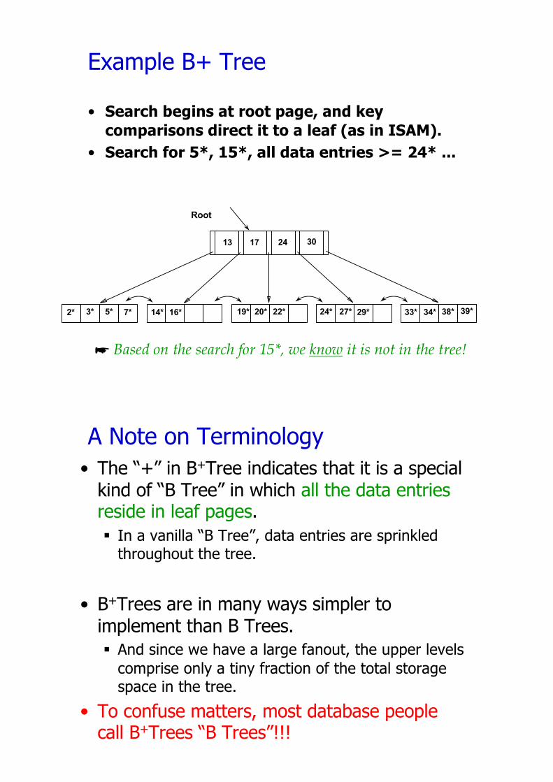
Example B+ Tree

• Search begins at root page, and key

comparisons direct it to a leaf (as in ISAM).

• Search for 5*, 15*, all data entries >= 24* ...

! Based on the search for 15*, we know it is not in the tree!

Root

17 24 30

2* 3* 5* 7* 14* 16* 19* 20* 22* 24* 27* 29* 33* 34* 38* 39*

13

A Note on Terminology• The “+” in B+Tree indicates that it is a special

kind of “B Tree” in which all the data entries reside in leaf pages.§ In a vanilla “B Tree”, data entries are sprinkled

throughout the tree.

• B+Trees are in many ways simpler to implement than B Trees. § And since we have a large fanout, the upper levels

comprise only a tiny fraction of the total storage space in the tree.

• To confuse matters, most database people call B+Trees “B Trees”!!!

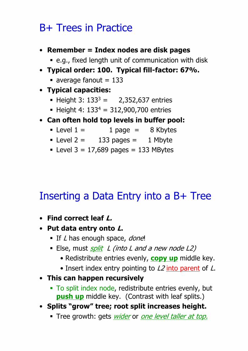
B+ Trees in Practice

• Remember = Index nodes are disk pages

§ e.g., fixed length unit of communication with disk• Typical order: 100. Typical fill-factor: 67%.

§ average fanout = 133• Typical capacities:

§ Height 3: 1333 = 2,352,637 entries§ Height 4: 1334 = 312,900,700 entries

• Can often hold top levels in buffer pool:

§ Level 1 = 1 page = 8 Kbytes§ Level 2 = 133 pages = 1 Mbyte§ Level 3 = 17,689 pages = 133 MBytes

Inserting a Data Entry into a B+ Tree

• Find correct leaf L.

• Put data entry onto L.

§ If L has enough space, done!§ Else, must split L (into L and a new node L2)

• Redistribute entries evenly, copy up middle key.• Insert index entry pointing to L2 into parent of L.

• This can happen recursively

§ To split index node, redistribute entries evenly, but push up middle key. (Contrast with leaf splits.)

• Splits “grow” tree; root split increases height.

§ Tree growth: gets wider or one level taller at top.

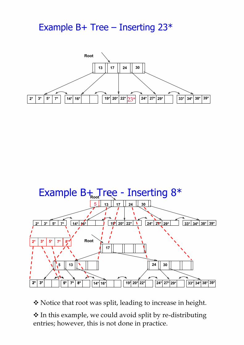
Example B+ Tree – Inserting 23*

Root

17 24 30

2* 3* 5* 7* 14* 16* 19* 20* 22* 24* 27* 29* 33* 34* 38* 39*

13

23*

Example B+ Tree - Inserting 8*

" Notice that root was split, leading to increase in height.

" In this example, we could avoid split by re-distributing entries; however, this is not done in practice.

Root

17 24 30

2* 3* 5* 7* 14* 16* 19* 20* 22* 24* 27* 29* 33* 34* 38* 39*

13

2* 3* 5* 7* 8*

2* 3* 7*5* 8*

5

24 30

14* 16* 19* 20* 22* 24* 27* 29* 33* 34* 38* 39*

135

2* 3* 7*5* 8*

Root

17

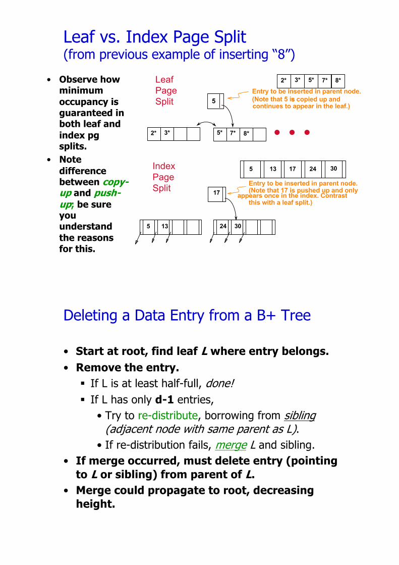
Leaf vs. Index Page Split (from previous example of inserting “8”)

• Observe how minimum

occupancy is

guaranteed in both leaf and

index pg splits.

• Note

difference between copy-up and push-up; be sure you understand

the reasons

for this.

5

Entry to be inserted in parent node.

(Note that 5 iscontinues to appear in the leaf.)

s copied up and

2* 3* 5* 7* 8* …Leaf Page Split

2* 3* 5* 7* 8*

5 24 3013

appears once in the index. Contrast17

Entry to be inserted in parent node.(Note that 17 is pushed up and only

this with a leaf split.)

17 24 3013Index Page Split

5

Deleting a Data Entry from a B+ Tree

• Start at root, find leaf L where entry belongs.

• Remove the entry.

§ If L is at least half-full, done! § If L has only d-1 entries,

• Try to re-distribute, borrowing from sibling(adjacent node with same parent as L).

• If re-distribution fails, merge L and sibling.• If merge occurred, must delete entry (pointing

to L or sibling) from parent of L.

• Merge could propagate to root, decreasing

height.

Root

17

24 30

19* 20* 22* 24* 27* 29* 33* 34* 38* 39*

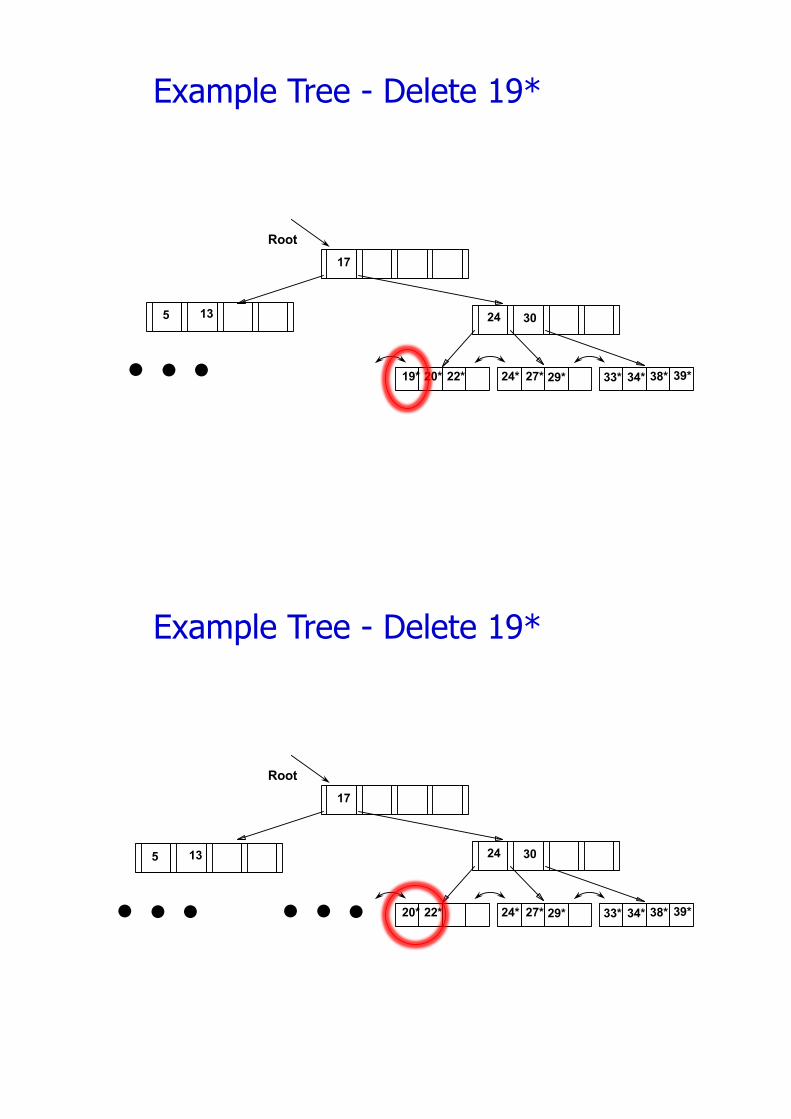
Example Tree - Delete 19*

���

5 13

Root

17

24 30

20* 22* 24* 27* 29* 33* 34* 38* 39*

Example Tree - Delete 19*

������

5 13

Root

17

24 30

20* 22* 24* 27* 29* 33* 34* 38* 39*

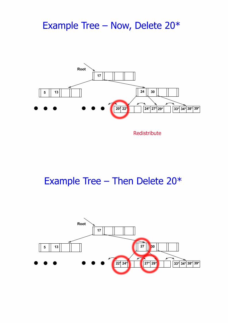
Example Tree – Now, Delete 20*

������

5 13

Redistribute

Root

17

27 30

22* 24* 27* 29* 33* 34* 38* 39*

Example Tree – Then Delete 20*

������

5 13

Root

17

27 30

22* 27* 29* 33* 34* 38* 39*

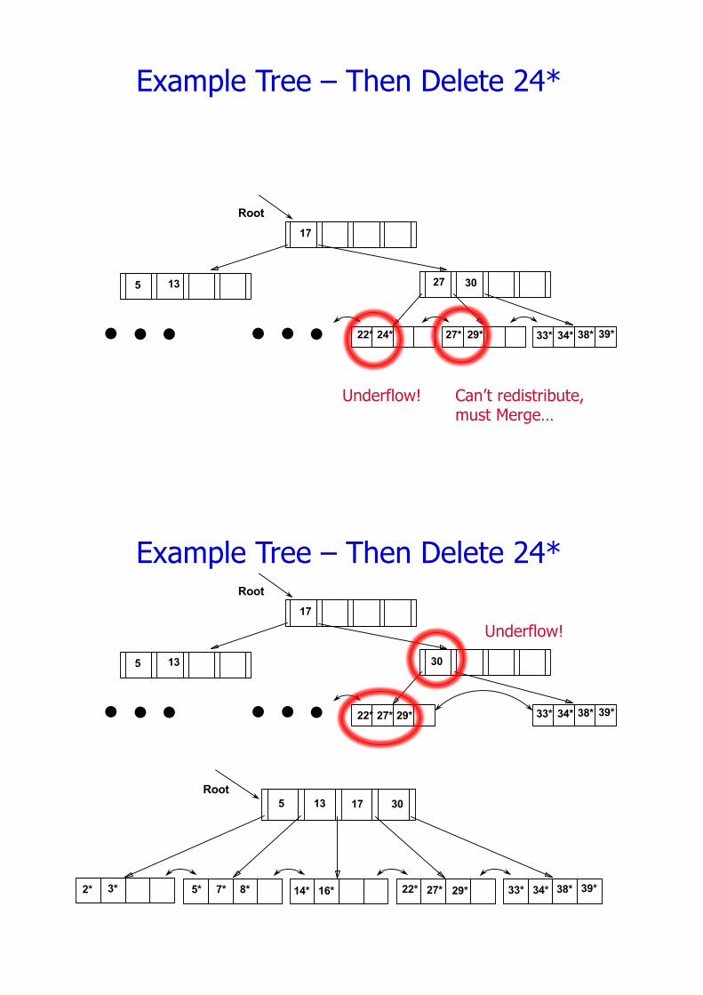
Example Tree – Then Delete 24*

���Underflow!

24*

Can’t redistribute,must Merge…

���

5 13

Root

17

30

22* 27* 29* 33* 34* 38* 39*

Example Tree – Then Delete 24*

���

Underflow!

���

5 13

Root

30135 17

2* 3* 7* 14* 16* 22* 27* 29* 33* 34* 38* 39*5* 8*

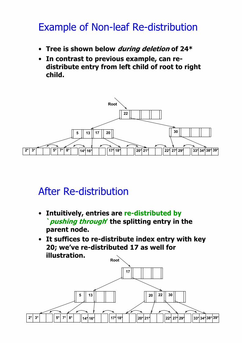
Example of Non-leaf Re-distribution

• Tree is shown below during deletion of 24*

• In contrast to previous example, can re-

distribute entry from left child of root to right

child.

Root

135 17 20

22

30

14* 16* 17* 18* 20* 33* 34* 38* 39*22* 27* 29*21*7*5* 8*3*2*

After Re-distribution

• Intuitively, entries are re-distributed by

`pushing through’ the splitting entry in the

parent node.

• It suffices to re-distribute index entry with key

20; we’ve re-distributed 17 as well for

illustration.

14* 16* 33* 34* 38* 39*22* 27* 29*17* 18* 20* 21*7*5* 8*2* 3*

Root

135

17

3020 22

A Note on `Order’• Order (d) concept replaced by physical space

criterion in practice (`at least half-full’).

§ Index pages can typically hold many more entries than leaf pages.

§ Variable sized records and search keys mean different nodes will contain different numbers of entries.

§ Even with fixed length fields, multiple records with the same search key value (duplicates) can lead to variable-sized data entries (if we use Alternative (3)).

• Many real systems are even sloppier than this -

-- only reclaim space when a page is

completely empty.

Introduction to Hash-based Indexes

• Hash-based indexes are best for equality selections.

Cannot support range searches.

• Static and dynamic hashing techniques exist; trade-

offs similar to ISAM vs. B+ trees.

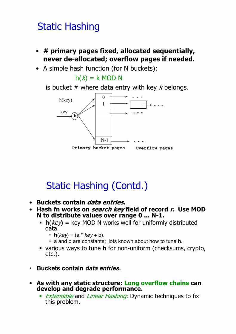
Static Hashing

• # primary pages fixed, allocated sequentially,

never de-allocated; overflow pages if needed.

• A simple hash function (for N buckets):h(k) = k MOD N

is bucket # where data entry with key k belongs.h(key)

hkey

Primary bucket pages Overflow pages

10

N-1

Static Hashing (Contd.)• Buckets contain data entries.• Hash fn works on search key field of record r. Use MOD

N to distribute values over range 0 ... N-1.

§ h(key) = key MOD N works well for uniformly distributed data.

• h(key) = (a * key + b).• a and b are constants; lots known about how to tune h.

§ various ways to tune h for non-uniform (checksums, crypto, etc.).

• Buckets contain data entries.

• As with any static structure: Long overflow chains can develop and degrade performance.

§ Extendible and Linear Hashing: Dynamic techniques to fix this problem.

Extendible Hashing• Situation: Bucket (primary page) becomes full.

§ Want to avoid overflow pages

• How about we add more buckets (i.e., increase “N”)?

§ Okay, but need a new hash function!

• Doubling # of buckets makes this easier

§ Say N values are powers of 2 – how to do “mod N”?§ What happens to hash function when you double “N”?

• Problems with Doubling

§ Don’t want to have to double the size of the file.§ Don’t want to have to move all the data.

Extendible Hashing (continued)• Idea: Add a level of indirection!

• Use directory of pointers to buckets,

• Double # of buckets by doubling the directory

§ Directory much smaller than file, so doubling it is much cheaper.

• Split only the bucket that just overflowed!

§ No overflow pages!§ Trick lies in how hash function is adjusted!

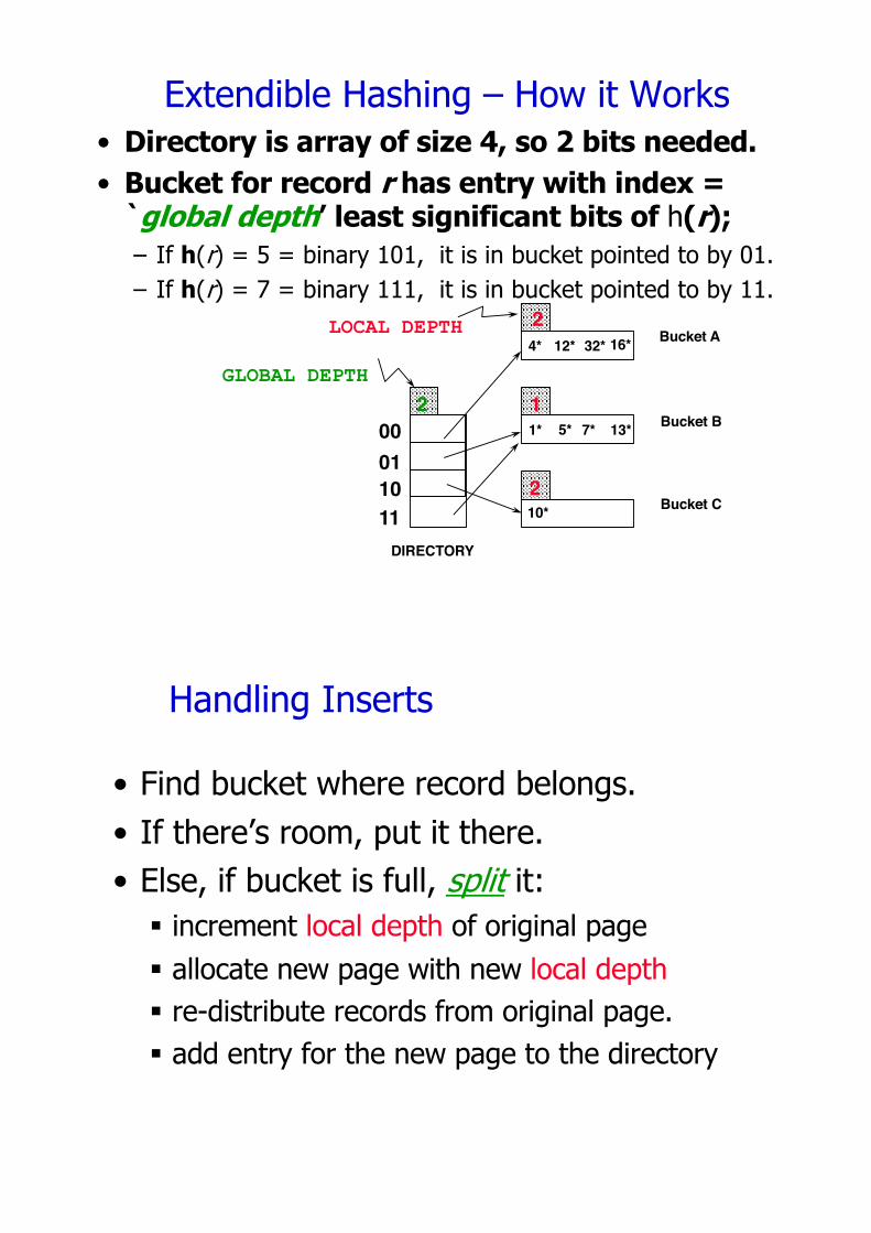
Extendible Hashing – How it Works

00011011

2GLOBAL DEPTH

DIRECTORY

13*

2

1

2

LOCAL DEPTH Bucket A

Bucket B

Bucket C10*

1* 7*

4* 12* 32* 16*

5*

• Directory is array of size 4, so 2 bits needed.

• Bucket for record r has entry with index = `global depth’ least significant bits of h(r);

– If h(r) = 5 = binary 101, it is in bucket pointed to by 01.– If h(r) = 7 = binary 111, it is in bucket pointed to by 11.

Handling Inserts

• Find bucket where record belongs.• If there’s room, put it there.• Else, if bucket is full, split it:

§ increment local depth of original page§ allocate new page with new local depth§ re-distribute records from original page.§ add entry for the new page to the directory

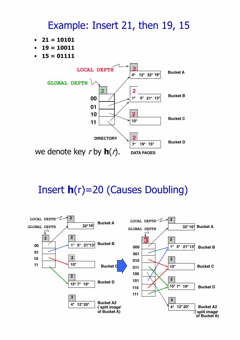
Example: Insert 21, then 19, 15

13*00011011

2

2

LOCAL DEPTH

GLOBAL DEPTH

DIRECTORY

Bucket A

Bucket B

Bucket C

2Bucket D

DATA PAGES

10*

1* 7*

24* 12* 32* 16*

15*7* 19*

5*

we denote key r by h(r).

• 21 = 10101

• 19 = 10011

• 15 = 01111

1221*

24* 12* 32*16*

Insert h(r)=20 (Causes Doubling)

00011011

2 2

2

2

LOCAL DEPTH

GLOBAL DEPTHBucket A

Bucket B

Bucket C

Bucket D

1* 5* 21*13*

10*

15* 7* 19*

(`split image'of Bucket A)

20*

3Bucket A24* 12*

of Bucket A)

3Bucket A2

(`split image'4* 20*12*

2

Bucket B1* 5* 21*13*

10*

2

19*2

Bucket D15* 7*

332*16*

LOCAL DEPTH

000001010011100101110111

3GLOBAL DEPTH

3

32*16*

Bucket C

Bucket A

Points to Note

• 20 = binary 10100. Last 2 bits (00) tell us r belongs

in either A or A2. Last 3 bits needed to tell which.

§ Global depth of directory: Max # of bits needed to tell which bucket an entry belongs to.

§ Local depth of a bucket: # of bits used to determine if an entry belongs to this bucket.

• When does bucket split cause directory doubling?

§ Before insert, local depth of bucket = global depth. Insert causes local depth to become > global depth; directory is doubled by copying it over and `fixing’ pointer to split image page.

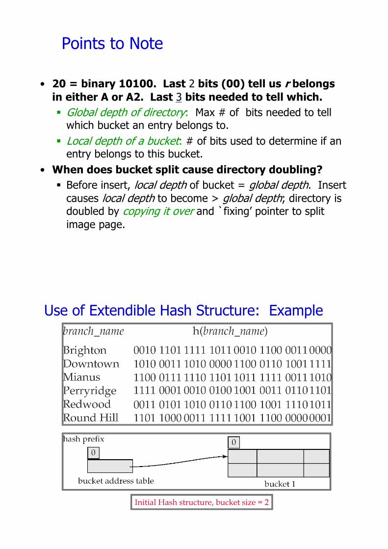
Use of Extendible Hash Structure: Example

Initial Hash structure, bucket size = 2

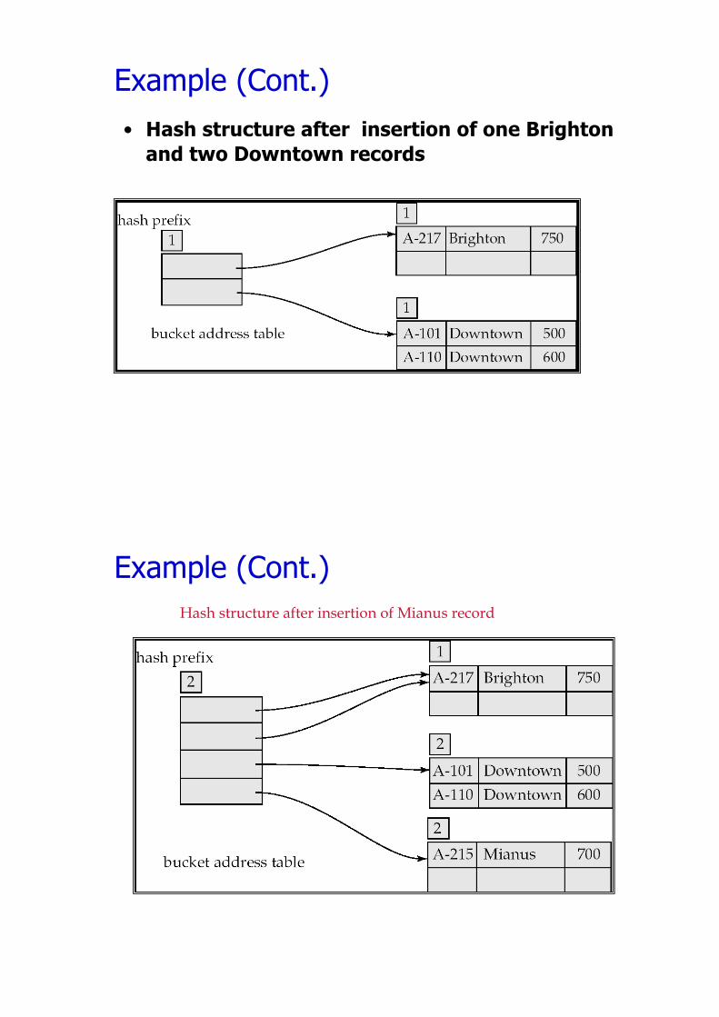
Example (Cont.)• Hash structure after insertion of one Brighton

and two Downtown records

Example (Cont.)Hash structure after insertion of Mianus record

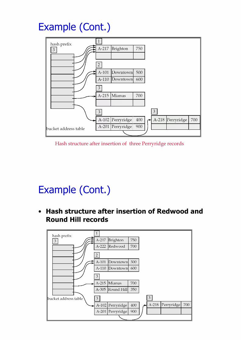
Example (Cont.)

Hash structure after insertion of three Perryridge records

Example (Cont.)

• Hash structure after insertion of Redwood and

Round Hill records

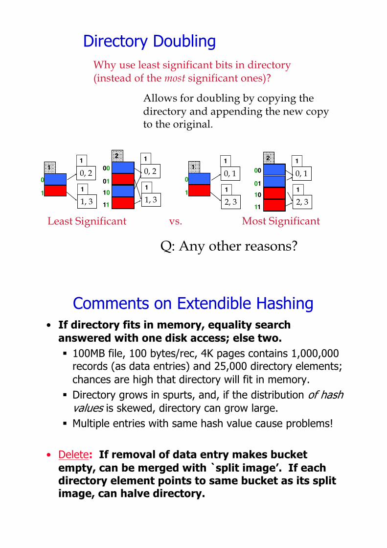
Directory Doubling

00

0110

11

2

Why use least significant bits in directory(instead of the most significant ones)?

vs.

0

1

1

0

1

1

Least Significant Most Significant

0, 2

1, 3

1

1

0, 2

1, 3

1

1

0, 1

2, 3

1

1

00

0110

11

2

0, 1

2, 3

1

1

Allows for doubling by copying the directory and appending the new copy to the original.

Q: Any other reasons?

Comments on Extendible Hashing• If directory fits in memory, equality search

answered with one disk access; else two.

§ 100MB file, 100 bytes/rec, 4K pages contains 1,000,000 records (as data entries) and 25,000 directory elements; chances are high that directory will fit in memory.

§ Directory grows in spurts, and, if the distribution of hash values is skewed, directory can grow large.

§ Multiple entries with same hash value cause problems!

• Delete: If removal of data entry makes bucket

empty, can be merged with `split image’. If each

directory element points to same bucket as its split

image, can halve directory.

Summary

• Tree-structured indexes are ideal for range-

searches, also good for equality searches.

• ISAM is a static structure.

§ Only leaf pages modified; overflow pages needed.§ Overflow chains can degrade performance unless size of

data set and data distribution stay constant.• B+ tree is a dynamic structure.

§ Inserts/deletes leave tree height-balanced; log F N cost.§ High fanout (F) means depth rarely more than 3 or 4.§ Almost always better than maintaining a sorted file.

Summary (Contd.)

§ Typically, 67% occupancy on average.§ Usually preferable to ISAM, modulo locking

considerations; adjusts to growth gracefully.§ If data entries are data records, splits can change

rids!• Other topics:

§ Key compression increases fanout, reduces height.§ Bulk loading can be much faster than repeated inserts

for creating a B+ tree on a large data set.• Most widely used index in database management

systems because of its versatility. One of the

most optimized components of a DBMS.

Summary – Hash Indexes• Hash-based indexes: best for equality searches,

cannot support range searches.

• Static Hashing can lead to long overflow chains.

• Extendible Hashing avoids overflow pages by splitting

a full bucket when a new data entry is to be added to

it. (Duplicates may require overflow pages.)

§ Directory to keep track of buckets, doubles periodically.§ Can get large with skewed data; additional I/O if this does

not fit in main memory.• “Linear hashing” solves some problems of Extendible

hashing – not covered in this course, but check out

book section 11.3 – it’s very cool!

Summary

• Index Definition in SQL

• Create an index§ create index <index-name> on <relation-name>

(<attribute-list>)

§ E.g.: create index b-index on branch (branch_name)• Use create unique index to indirectly specify and

enforce the condition that the search key is a candidate key is a candidate key.

§ Not really required if SQL unique integrity constraint is supported

• To drop an index

§ drop index <index-name>• Most database systems allow specification of type

of index, and clustering.