DATABASE SYSTEM AND APPLICATIONS DEVELOPED FOR RESERVOIR ... · DATABASE SYSTEM AND APPLICATIONS DEVELOPED FOR RESERVOIR ... Energy Development Corporation for reservoir engineering

GEOTHERMAL TRAINING PROGRAMME Reports 2003Orkustofnun, Grensásvegur 9, Number 4IS-108 Reykjavík, Iceland

33

DATABASE SYSTEM AND APPLICATIONS DEVELOPED FORRESERVOIR MODELLING AND MONITORING OF

GEOTHERMAL FIELDS IN THE PHILIPPINES

Jaime Jemuel C. Austria, Jr.Reservoir and Resource Management Department

PNOC – Energy Development CorporationPNPC Complex, Merritt Road, Ft. Bonifacio

Makati City, Metro ManilaPHILIPPINES

[email protected]

ABSTRACT

The present database system of PNOC – Energy Development Corporation forreservoir engineering is improved to support rapid correlation of diverse sets ofreservoir data for model conceptualization and reservoir modelling. Simpleapplication programs for data visualization were created to show how databasefunctionality can be enhanced from mere data storage into a useful tool for reservoirsimulation and monitoring.

Logical data blocks are drawn from an Oracle database on the fly within a UNIX shellscript to create dynamic line graphs and contour planes of temperature and pressureproviding basic graphic representation of the reservoir. Developer forms are createdfor graphical retrieval and handling of data.

1. INTRODUCTION

Management of a geothermal reservoir relies on adequate information on the geothermal system(Stefánsson and Steingrímsson, 1980). The prediction of the behaviour of a reservoir during theproduction stage depends on the conceptual model of that reservoir, the governing physical processes, andthe quality of data used in the interpretation. Good quality of data is not an assurance of a perfectconceptual model but is important in realizing that goal (Grant et al., 1982).

The study deals with the optimization of the design of, and inclusion of, new application tools to thepresent database system of the Reservoir and Resource Management Department (RRMD) ofPNOC–Energy Development Corporation (PNOC-EDC). The RRMD database has been redesigned tocapture more accurate information on geothermal systems, and to support the data requirements ofreservoir modelling and field monitoring.

At present, the database contains information from close to 350 wells that have been drilled into thegeothermal fields of Bacon-Manito, Palinpinon, Tongonan, and Mindanao; and into exploration areas of

Austria Report 434

Northern Negros, Mt. Labo, Central Leyte, and Southern Leyte. The data in all geothermal fields arecontained in spreadsheets with a file-based structure. In 1997, a decision was made to create a datamanagement system for geothermal data for all project locations to improve the quality of data used formanaging the reservoir. Web-based database set-up using thin-client architecture was chosen to be idealfor the collection of data from remote locations (Zapanta et al., 1999). As a result, a geothermal databasemanagement system broadcasted on the web was adopted for RRMD.

Geothermal data from different areas are standardized and collected in a central database in FortBonifacio, Makati. Collection of data includes contextual information such as wellhead and well trackcoordinates, and boundaries of pads, sectors and projects. Numerical data from temperature, pressure,spinner, calliper, and sonic logs can be downloaded and used to create graphs. Maps of well locations ofdifferent geothermal projects are available in static hypertext mark-up language (HTML) format. Welltest interpretations provide information regarding feed zone locations, injectivity indices, permeabilitythickness and skin values.

Access to the database is comprehensive as it allows personnel, with an approved internet protocol (IP)address and valid user ID, to view and update information as needed by using only their web browsers.

The study includes a review of the current reservoir engineering database setup for PNOC-EDC againsta data management model for reservoir simulation.

The database has application forms to perform basic calculations like data interpolation for temperatureand pressure. The database management system also has basic computational tools, but its architecturehas to be refined to provide better collection of data for reservoir conceptualization and modelling.Moreover, database application programs need to be developed to provide a basic graphical representationof the reservoir data.

The database and applications were developed using the software installed on the UNIX server, calledStrokkur, at Orkustofnun. These UNIX-based programs were accessed from a personal computeroperating on Windows XP 2000 by installing an X-windows terminal on the PC to emulate the UNIXenvironment.

2. BACKGROUND OF STUDY

2.1 Current web-based database system of PNOC-EDC for reservoir engineering

In 1997, the Reservoir and Resource Management Department of PNOC - EDC, developed a web-basedgeothermal database management system using thin-client architecture to handle large volumes of datacoming from remote and geographically diffuse project locations. Data from these sources come inheterogeneous types and formats.

Database management systems using thin-client architecture operate like a corporate intranet withdatabase connectivity. Transmission control protocol / internet protocol (TCP/IP) is used as acommunications protocol by the intranet to provide hypertext transfer protocol (HTTP) servicescontaining information from the database to users.

TCP/IP is a two-layer program. The upper layer, TCP, manages the assembly of a message into smallerpackets that are transmitted over the Internet and received by a TCP layer that reassembles the packets intothe original message. The lower layer, IP, handles the address part of each packet to make sure it gets tothe right destination. Each gateway computer on the network checks this address to see where to forwardthe message.

Report 4 Austria35

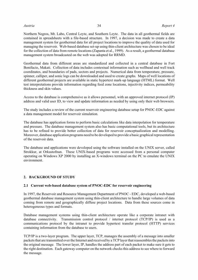
FIGURE 1: User interface for RRMD web-based database

Thin-client architecturei s a mul t i - l eve larchi tec ture wi thdistributed computingpower. Thin-clientarchitecture has a web-browser client on thefront-end, an applica-tion server in themiddle, and a databaseserver on the back-end.The client portion, asshown in Figure 1, isan entry screen formaking requests andreceiving services, suchas a web page, from acomputer functioningas an application serverin the network.

2.2 Web-based database architecture and its advantages

The first tier in a multi-tier web-based database system is the user interface. In the RRMD configuration,a web browser that comes bundled with preinstalled application programs in desktops and mobilecomputers is used as a user interface. Computer users from Fort Bonifacio, Makati central office, andfrom satellite offices in Tongonan, Palinpinon, Bacon-Manito, and Mindanao geothermal projects canaccess data using the web browsers on their computers as long as they are connected to the LAN andWAN.

The second tier is an application server containing application programs and forms. An application servermay be any server supporting web services and web scripting languages like HTML and JavaScript. Inthe RRMD configuration, the second tier is a Microsoft NT computer running Internet Information Server(IIS). The data entry and retrieval forms are designed using Microsoft FrontPage and JavaScript.

The third tier is a web server which is an HTTP server that has object database connectivity (ODBC).ODBC allows creation of HTML documents using data from a relational database. In the RRMD set-up,Oracle Webserver’s Listener triggers the Oracle web agent when a database connection is requested, tomake a connection to the Oracle database. Stored procedures written in procedural language/structuredquery language (PL/SQL), which provide program logic, are compiled in an Oracle 8.05 server to createdynamic HTML pages, and storage for dynamic data in relational tables.

The fourth tier that completes the architecture is the geothermal data which is stored in an Oracle relationaldatabase management system (RDBMS). The Oracle RDBMS runs on SUN’s Solaris platform.

The main advantage of a web-based database system is the database and analysis modules are stored ina centralized system. Updates to programming applications only have to be made on the server. Noadditional programs are needed at remote client desktop computers. Changes, whether in the data, forms,or application programs, are dynamically made available to all users at their web browsers without havingany need to install additional programs.

Austria Report 436

3. DEVELOPMENT OF GEOTHERMAL DATABASE

3.1 Objective of the study

This UNU geothermal project deals primarily with the improvement of the present database system toextend its function as storage of archival geothermal data into an effective tool for reservoirconceptualization and modelling. The database was restructured to be more fitting for databaseapplication programs that were developed to facilitate the rapid correlation of different sets of reservoirdata and provide visualization of different reservoir parameters.

3.2 Effective geothermal database design

A systematic collection of data is important in understanding a geothermal resource in its natural state andin monitoring changes of the resource during exploitation. The database provides a structure forsystematic gathering of information. By placing data in a database, standards are imposed on data thatimprove the quality of data and make data easily accessible in the future. Data have to be interpreted andanalyzed before a conceptual model can be developed. A conceptual model represents understanding ofthe resource at a given time based on a particular set of data. In order to have better understanding of aresource, all available data sets are used to create many conceptual models. Different models of theresource are integrated to create an integral model of the resource. The data management system musttherefore provide a flexible retrieval and comparison of data from different sources for data analysis.Furthermore, the data management system must allow data to be shared with all experts who are involvedwith the analysis of data (Anderson, 1995).

Management decisions regarding the resource are made based on this integral model. An effective datamanagement system should indicate assumptions made during development of the conceptual model sothat models can be updated easily; and decisions will be based on known assumptions. Moreover, a sounddata management system must ensure that data can be improved upon, and improvements are noted whileoriginal data remains the same (Anderson, 1995).

3.3 Data review based on role of data management in numerical simulation

Data modelling is important to define areas where the present data management system is adequate andareas where it needs improvement. The reservoir simulation experience of PNOC-EDC is evaluatedagainst the data flow diagram showing how data management and related software is used in reservoirsimulation (Figure 2).

Batches of raw data verified to be correct are sent from field offices to the Makati head office byelectronic-mail for uploading to the database. The architecture of the database allows for interactiveupdating from remote locations using the web browser. However, due to bandwidth limitation from thecentral office to remote locations, this method is slow and is not practical. Data from the field offices, infile-based spreadsheet format and in flat file databases, are recorded on recordable compact discs forarchival purposes. Meanwhile, electronic logging data are stored on tape cartridges.

Data viewing is done using the RRMD web page interface. After data are uploaded to the database, userswith a proper IP and authorized user ID can view a web report from computers that are part of the LANand WAN. The reports can be saved directly as HTML, or can be copied and pasted into a text editor.

The database, ideally, is linked seamlessly to various stand-alone reservoir engineering programs used todetermine stable formation temperature, interpret well tests, and simulate wellbore conditions. However,the current reservoir database is not linked seamlessly to any stand-alone reservoir application software.Data is searched from the database and downloaded before it can be used as input for a well test analysis,wellbore modelling or other software.

Report 4 Austria37

Data entry and retrieval usingAPPLICATION SOFTWARE

Preprocessor tosimulator

RESERVOIRSIMULATOR

Postprocessor tosimulator

Various stand-aloneprograms

DATADISPLAY

Temperature prediction softwareWell test analysis softwareWellbore simulation softwareDischarge ratio softwareBore output computation

Temperature and pressure graphsTemperature and pressure cross sectionsProduction trends

Drilling dataDirectional survey dataCasing and liner configurationsCompletion test dataTemperature and pressure surveysBore output measurements

Verificationfieldsheets and

worksheets

Storage inDATABASE REPORTS

Offline storage ofdata in cd-romand tape drives

RAW DATAfrom the field

Welltrack coordinatesBasic well informationBlockage summaryCasing and liner summary

RESULTS

FIGURE 2: Role of data management and related software inreservoir simulation patterned after GeothermEx Inc. (1995)

The database, ideally, is linked seamlessly to a reservoir simulator pre-processor via the applicationsoftware. In this manner, the database is able to supply information required for a numerical simulationmodel, which is nearly the entire database collected in the course of exploration, drilling, well logging,well testing and production/injection operations over the life of the project. In this aspect, much workneeds to be done on the RRMD database before it can generate sufficient data for reservoir modelconceptualization, or perhaps create a preliminary input deck for the simulator.

The reservoir simulator should be able to pass simulated data to a postprocessor for model calibration.TETRAD, the reservoir simulator currently being used, has a postprocessor that allow results of modellingto be viewed graphically and calibrated against measured data.

The database should be able to display graphics on the fly using data from the database. Currently,temperature and pressure contours and cross-sections are prepared manually using third-party graphingand contouring applications. The current reservoir database does not have any capability to display datadynamically.

3.4 Tools used for database and applications development

Assortments of programming languages and graphing tools are used to develop the database and theapplications. These include SQL+, Oracle SQL* Loader, UNIX shell scripting, AWK, Oracle Developer,GNUPLOT, and GMT.

The database engine used is Oracle8i Enterprise Edition Release 8.1.7.3.0. Being a relational database,information is stored into Oracle’s tables with the ability to link data between tables at the record level.

Austria Report 438

SQL+ is used to create the database. SQL+, or Structured Query Language Plus, is the language used forrelational database development. The language consists of statements to insert, update, delete, query andprotect data. The language is non-procedural which means users only have to specify which data theywant and how this data must be found. Oracle SQL* Loader is used to load data in batches. SQL*Loaderis an Oracle-supplied utility that allows the user to load data from a flat file into one or more databasetables (Moran and Dimmick, 1987).

SQL+ statements are embedded in simple programs written using UNIX shell scripts. The shell scriptsrun embedded SQL+ statements to query the database and spool selected data into a file. The shell scriptautomates the plotting program to use the input data and to display the data in graphical form. Data filesfrom the Oracle database are formatted into the desired data input structure using AWK. AWK, namedafter its developers Aho, Weinberger, and Kernighan, is a UNIX utility that uses regular expression forpattern matching. An AWK program searches a set of patterns and actions that tell what to look for in theinput data and what to do when it is found. The action language looks like C but there are no declarations,and strings and numbers are the built-in type (Aho et al., 1988; Dougherty, 1992).

Forms and reports interface applications are created using Oracle Developer. Oracle Forms can be usedto view, insert, and edit data while Oracle Reports allows the user to access data and to publish it(Lakshman, 2000).

For the X-Y plots, GNUPLOT is used to create the graphs using input data from the database. GNUPLOTis a command-line driven interactive plotting utility that runs on UNIX, MSDOS, and VMS platforms.The software is copyrighted but is freely distributed. GNUPLOT can handle both curves (2 dimensions)and surfaces (3 dimensions).

Generic Mapping Tools (GMT) is used to generate the contours. GMT is a free software package, withGeneral Public License, that can be used to manipulate columns of tabular data, time-series, and griddeddata sets, and display these data in a variety of forms ranging from simple X-Y plots to maps and colour,perspective and shaded-relief illustrations (Wessel and Smith, 1998).

All of the software used are installed on the Strokkur server of Orkustofnun. To run these UNIX-basedprograms on a personal computer operating on Windows XP 2000, an X-windows terminal is installedfirst on the PC to emulate the UNIX environment.

3.5 Database design and creation

In designing the database, key information required for successful resource management as described byStefánson and Steingrímsson (1980) is considered. These include:

• Knowledge on the volume, geometry, and boundary conditions of a reservoir;• Knowledge on the properties of the reservoir rock, i.e. permeability, porosity, density, heat capacity

and heat conductivity; and• Knowledge on the physical conditions in a reservoir, which are determined by temperature and

pressure distribution.

There is a conscious effort to separate original data from derived data, to include the source ofinterpretations, and indicate the accuracy of measurements. The improved design also uses strictly IDnumbers as the primary key instead of well-names to describe relationships between different data sets.

3.5.1 Well location module

The Location module includes tables for pad, sector, project, and cellar that describe the geographical

Report 4 Austria39

LOGF

DS

WELLPADWELLNAMEXYZMEASDEPTHWHEAD

WELL

PROJECTPR0JCODEADDRESSXYRADIUSREMARKS

PROJECT

SECTORPROJECTSECTCODEXYRADIUSREMARKS

SECTOR

PADSECTORPADCODEXYRADIUSREMARKS

CELLARPADCELLARCODEXYRADIUS

CELLAR

LOGWELLCONDITIONTOOLDATE_STARTDATE_ENDSHIFTLOGDIRECTIONENGR

WELLSTIM

DDATA

LOGDEPTHVALUE

TDATA

LOGTIMEVALUE

WELLUSE

BOMWELLDATE_STARTOPENINGWHPENTHALPYWATERFMASSFSTEAMFPOWERFLAG

BOM

TOOLTOOLNAMETOOLTYPEBRANDDESCRIPTION

TOOLCALIBRATETOOLDATECALIBRANGEMINRANGEMAXREFERENCE

CALIBRATE

CALIBRATETEMPPRESSERROR

DEFLECTREPAIRS

CALIBRATEDATERESULT

CBL

LOGPLOTFILEPLOTDESC

PATSPLOTS

WELLUSEWELLWELLUSAGEWELLSTATDATETIMEWHP

LOCATION

PZ

LOGGING

WELLLOGTOOLSURDATETOOLDIAMMCDSTATUS

BLOCKAGES

COMPLETIONCOMPLETIONWELLDATE_STARTDATE_ENDINJECTIVITYINJDEPTHMAXWHPKHSKIN

PRODUCTION

PADDSWELLDSMDDSVDDSMNDSMEDOGLEGDRIFTUSER_INITIALDATE_STARTUSER_CHANGEDATE_CHANGE

WELLCOMPLETIONPZFROMPZTOPZCODESOURCEREMARKS

WELL

WELLSTIMWELLEQUIPTYPEDATE_STARTDATE_ENDOPHRSOPERENGRMAXPRESSFUELITREMARKS

WELLKOPMODACCURACYDATE_EQNMEVSRD_0MEVSRD_1MEVSRD_2MEVSRD_3MEVSRD_4MNVSRD_0MNVSRD_1MNVSRD_2MNVSRD_3MNVSRD_4MMDVSRD_0MMDVSRD_1MMDVSRD_2MVDVSRD_0MVDVSRD_1SOURCE

TRACKPOLYSTABLETEMP STABLEPRES

WELLDATE_EQNSTPRES_0STPRES_1STPRES_2STPRES_3FLAGSOURCE

STABLETEMPEQN STABLEPRESEQN

WELLDATE_INTREDUCEDEPTHPRESSURESOURCE

CBLLOGCBLFROMCBLTOBONDPCT

EQUATIONS

CASINGDRILLJOBWELLCBLDATE_STARTDATE_ENDCSGTYPEODIDTOPBOTTOM

DRILLJOB CASING

DRILLING

DRILLJOBWELLACTIVITYDATE_STARTDATE_ENDDEPTH_STARTDEPTH_ENDRIGPURPOSERKBCHF

WELLDATE_INTREDUCEDEPTHTEMPERATURESOURCE

WELLDATE_EQNSTEMP_0STEMP_1STEMP_2STEMP_3STEMP_4FLAGSOURCE

FIGURE 3: Entity-relationship diagram for reservoir engineering database

location of a well by area (see Figure 3). The tables in the Location module describe the location on a wellby giving its rough centre and radius.

• PAD table contains ID of pad and sector where pad belongs, name of pad, easting (x) and northing (y)coordinates of pad, radius of circular area and a remarks column describing the pad location.

• SECTOR table contains ID of sector and project where sector belongs, name of sector, easting (x) andnorthing (y) coordinates of centre of sector area, radius of sector area, and a remarks column for theofficial name of the sector.

• PROJECT table contains ID of project, official name of project, mailing address of project, easting(x) and northing (y) coordinates of centre of project area, estimated radius of project area, and aremarks column for the official name of the project.

• CELLAR table contains ID of cellar and pad where cellar belongs, name or code of the cellar, easting(x) and northing (y) coordinates of centre of cellar, and estimated radius of cellar area.

3.5.2 Drilling module

The Drilling module contains information about the drilling activity and the casing configuration of a well(see Figure 3).

Austria Report 440

• DRILLJOB table contains drilling ID, well ID, type of drilling activity, date of start and finish ofdrilling activity, initial and final depth of drilling, name of rig used for the activity, reason for activity,and distance from rotary table to wellhead.

• CASING table contains casing ID, ID of drill job, well ID, sonic log ID, date of start and finish ofsetting of casing, type of casing, outer diameter of casing or slotted liner, inner diameter of casing orslotted liner, top of casing, and bottom of casing.

3.5.3 Well module

The Well module has information about the wellhead coordinates, well track coordinates, results of welltests and stimulation activities done on a well (see Figure 3).

• WELL table contains ID of well and pad record where well belongs, nickname of well, easting (x),northing (y), and elevation (z) wellhead coordinates. Well coordinates are based on National Mappingand Resource Information Authority (NAMRIA) maps with a scale of 1:50,000, and use the Clarke1866 spheroid and Transverse Mercator projection as coordinates (Los Banos, pers. comm., 2003).The table also contains the total measured depth of well and ID of well head. WELL is a central tableto which all other tables are linked. Several views can be created to link WELL with tables describinglocation to speed up searches for a well by pad, sector, or project.

• COMPLETION table contains the interpreted results of a well completion test. A well completionincludes several tests like waterloss, injectivity, and pressure transients. COMPLETION stores the IDof the completion test and well, date of start and finish of well tests, injectivity index of well computedfrom injectivity tests, depth of setting of the pressure tool during injection test, maximum wellheadpressure during injection test, computed permeability thickness and skin.

• DS table contains results of directional surveys. DS is widely used in mapping applications whenprojections of well track of deviated wells are made on different surfaces and cross-sections. Entitiesin this table include the ID of the directional survey, the ID of the well where the survey was done,measured length along the casing and vertical depth where a directional survey point was taken, easting(x) and northing (y) coordinates of the point where the survey is taken, dogleg severity, drift angle,names of encoder or personnel who made changes to the record, and dates when record was inputtedor changed.

• PZ table includes permeable zones of a well interpreted from temperature, and in some cases, spinnerlogs. PZ contains the ID of the well where the log was done, completion ID when the permeable zoneis identified from a log during well completion, interval of permeable zones, rough classification ofthe permeable zone as major or minor, data source such as logs performed to identify a permeable zoneor a wellbore simulation, and author of interpretation.

• WELLSTIM table covers parameters measured when a well is initiated to discharge by aircompression. WELLSTIM contains the ID of well stimulation activity, the ID of the well beingdischarged, the type of equipment used to discharge the well, date of start and finish of well activity,total hours of operation, maximum pressure reached during compression, volume of fuel consumedby equipment, names of engineers and operators who carried out the project, and comments on howto improve the next discharge stimulation activity.

3.5.4 Production module

The Production module contains tables that describe the production history of wells, utilization ofproduction and re-injection wells, and measurements of well output (see Figure 3).

Report 4 Austria41

• WELLUSE table contains the ID record of well utilization, ID of the well, present use of the well (e.g.used for production, re-injection, or monitoring), status of the well (e.g. shut, in use for power plant,flowing, or bleed off), date and time of start of utilization, and wellhead pressure while being used.

• BOM table or bore output measurement table contains ID of bore output records and well, date of startof output measurement test, wellhead condition, computed enthalpy, water flow, mass flow, steamflow, and power output, and a flag for stable outputs that can be used for generating bore output curves.

3.5.5 Logging module

Logs give information on well performance and design. This information is necessary during drilling toavoid anticipated drilling difficulties, and to estimate success. Logs give information on structure,physical properties and performance penetrated by wells (Stefansson and Steingrímsson, 1980).

The Logs module contains information about geophysical logs such as temperature, pressure, spinner,sonic, calliper, blockage detection, and flow. The Logs module also contains a description of the toolsused for logging, results of calibration performed on a tool to keep it accurate, and records of repairs doneon tools. The modules for logging are designed to allow tracking the number of times a tool has been usedand the wells where it has been used. This feature is very important in tracing all the wells logged by atool that is giving wrong readings due to an off-calibration (see Figure 3).

• LOGF table contains the ID of the log and well, the condition of the well while it is being logged (e.g.shut, flowing, on-bleed), tool used for logging well, date of start and finish of logging activity, shiftvalue to correct for errors in zeroing to the reference point during logging, direction of log (e.g. logis made going up, going down or stationary), and names of loggers.

• DDATA table contains logging data against depth. Data from moving logs of temperature, pressure,and spinner against depth are stored in this table.

• TDATA table includes logging data against time or time series data. Data from stationary logs ofpressure like those performed during multi-rate injection and pressure transient tests are stored in thistable.

• TOOL table contains the ID of the tool, name of the tool, kind of tool (e.g. temperature, pressure,spinner, flow meter, neutron, gamma, resistivity, X-Y caliper, casing inspection or multifinger caliper),brand or manufacturer of the tool, and general description of the tool.

• BLOCKAGES table contains records of all blockages detected during a Go-devil, lead impressionblock, and sinker bar survey. BLOCKAGES contains the ID of the log and well, date of the log,outside diameter of the tool used, and depth where the blockage is detected. This table can be a partof the LOGF table.

• CBL table contains data on cement bond logs. CBL includes the ID of the log, the casing intervalwhere CBL is performed, and the quality of cement bond or percent bond index. This table can alsobe a part of the LOG table.

• PATSPLOTS table contains previous plots of logs performed on wells in HTML format.

• CALIBRATE, REPAIRS and DEFLECT tables contain information about calibration of tools,equations used in the calibration of tools, and details of repairs done on tools.

Austria Report 442

3.5.6 Equations module

The Equations module contains interpreted stable formation temperature and pressure from downhole logsand polynomial equations describing the stable profiles. There is also a table describing the well tracksusing polynomial equations. The equations module is mostly used for finding temperature and pressureof wells at different depths in the reservoir (see Figure 3).

• STABLETEMP and STABLEPRES tables contain stable formation temperature and pressure. Thetables have interpreted stable formation temperatures and pressures, depth where measurements aretaken, and the name of the person who made the interpretation.

• STABLETEMPEQN and STABLEPRESEQN tables contain equations of the polynomial fit lineto the interpreted stable formation temperature and pressure plots.

• TRACKPOLY table contains polynomial equations describing the welltrack. The polynomialequations relate easting, northing, measured depth, and vertical depth to absolute depth. The table alsostores the name of the person who created the polynomial fit.

The details of these tables are contained in the data dictionary included as Appendix I.

3.6 Techniques in data migration and population

Data relevant to the project were imported into the Strokkur server of Orkustofnun using Oracle’s importutility. Data from previous tables are migrated using SQL statements from the command line when thecolumns in the table have the same data types and field lengths.

Volumes of data in ASCII format are batch-loaded using SQL*Loader. AWK is used to format ASCIIdata into a structure readable by SQL*Loader. A feature of SQL*Loader, the control file, is written todescribe data for loading and which tables and columns will accept the data. After writing the control file,the load process is started by invoking SQL*Loader executable and pointing it to the control file. ASCIIdata is read by SQL*Loader and loaded into the database.

The design of a database is not a single and discrete phase of a data management project, therefore, controlscripts are kept in an archive folder in case the tables need to be dropped and rebuilt in the life cycle ofthe project.

4. DEVELOPMENT OF SIMPLE DATABASE APPLICATIONS

4.1 Development of temperature and pressure program

Graphing modules TPLOT and PPLOT are developed to give reservoir analysts a quick view of the plotof all available temperature and pressure data for all wells in the database. These modules displaydynamic two-dimensional plots of temperature and pressure for any given well within a given time frame.Updated temperature and pressure data are readily seen on the graphs when the graphs are generated againafter the changes are made.

The TPLOT program is capable of extracting temperature data from the database and generating a plotof temperature against depth. The PPLOT program, on the other hand, can produce a plot of pressureagainst depth (see Figures 4 and 5).

Report 4 Austria43

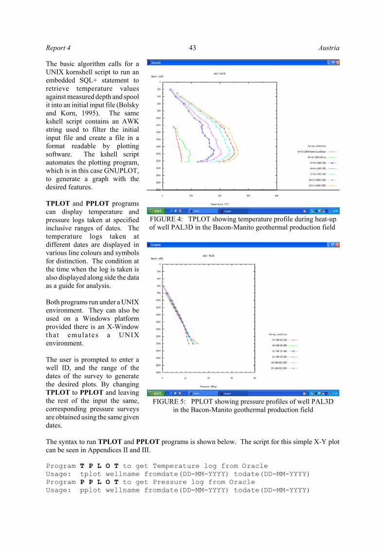
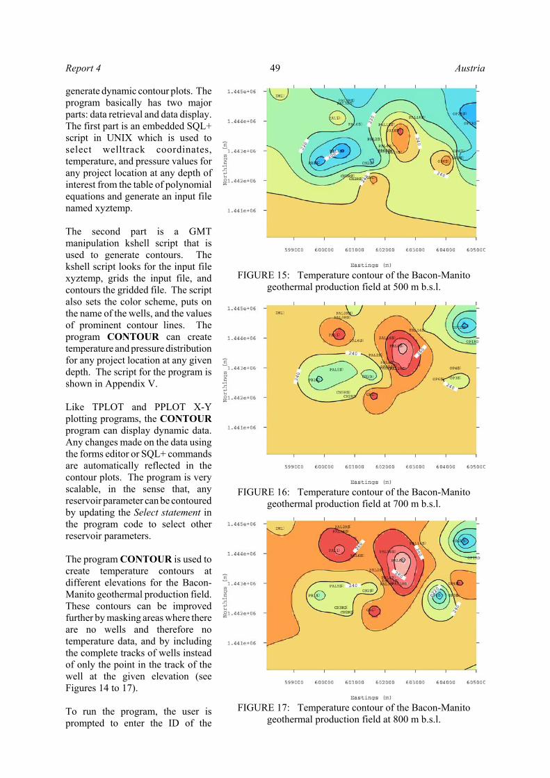
FIGURE 4: TPLOT showing temperature profile during heat-upof well PAL3D in the Bacon-Manito geothermal production field

FIGURE 5: PPLOT showing pressure profiles of well PAL3Din the Bacon-Manito geothermal production field

The basic algorithm calls for aUNIX kornshell script to run anembedded SQL+ statement toretrieve temperature valuesagainst measured depth and spoolit into an initial input file (Bolskyand Korn, 1995). The samekshell script contains an AWKstring used to filter the initialinput file and create a file in aformat readable by plottingsoftware. The kshell scriptautomates the plotting program,which is in this case GNUPLOT,to generate a graph with thedesired features.

TPLOT and PPLOT programscan display temperature andpressure logs taken at specifiedinclusive ranges of dates. Thetemperature logs taken atdifferent dates are displayed invarious line colours and symbolsfor distinction. The condition atthe time when the log is taken isalso displayed along side the dataas a guide for analysis.

Both programs run under a UNIXenvironment. They can also beused on a Windows platformprovided there is an X-Windowthat emula tes a UNIXenvironment.

The user is prompted to enter awell ID, and the range of thedates of the survey to generatethe desired plots. By changingTPLOT to PPLOT and leavingthe rest of the input the same,corresponding pressure surveysare obtained using the same givendates.

The syntax to run TPLOT and PPLOT programs is shown below. The script for this simple X-Y plotcan be seen in Appendices II and III.

Program T P L O T to get Temperature log from OracleUsage: tplot wellname fromdate(DD-MM-YYYY) todate(DD-MM-YYYY)Program P P L O T to get Pressure log from OracleUsage: pplot wellname fromdate(DD-MM-YYYY) todate(DD-MM-YYYY)

Austria Report 444

FIGURE 6: Water loss profile of well PAL4Dgenerated by TPLOT

FIGURE 7: Water loss and heat-up profile of well CN2RDgenerated from TPLOT

4.2 Practical applications of TPLOT and PPLOT

The simple programs TPLOT and PPLOT can be very useful tools for analyzing downhole logs.Behaviour of wells as inferred from downhole logs used as a basis to explain physical processes happeningdown in a geothermal reservoir. Graphs of temperature and pressure generated from TPLOT show howthe program can be useful in visualizing well behaviour from the logs.

The permeable zone can belocated from downhole logs, suchas successful water loss tests.

A profile of well PAL4D in theBacon-Manito geothermalproduction field (BGPF) shows awell warming by conduction aswater flows down the casing andcasing section (Figure 6). Belowthe region of slow warming, adepth is reached where thetemperature rises sharply. Wateris not moving at this section ofthe well below this water leveland is lost into formation.

A profile of CN2RD in the BGPFshows partial water loss in theupper zone (Figure 7). Reductionin flow as water flows down thewell leads to greater heating byconduction. The upper zone lossis indicated by steep change inthe thermal gradient. In this case,the upper zone is most likely themajor zone as most of the wateris lost in this part causingsignificant heating.

A profile of CN3D in the BGPFshows a step change intemperature indicating inflow ofhot water mixing with injectedcold water (Figure 8). Theinterval of log measurements hasto be closely spaced to be able toidentify the step change.

Formation temperature andpressure can be inferred fromdownhole logs if the well is shutlong enough to adjust to stabletemperature and pressure.However, temperature and pressure measurements from logs do not necessarily correspond to those of thereservoir. Correspondence depends strongly on the reservoir pressure gradient and distribution of feedzones.

Report 4 Austria45

06-03-1990-Waterloss-6bpm

06-03-1990-Waterloss-8bpm

Survey condition

FIGURE 8: Water loss and heat-up profile of well CN3Dgenerated from TPLOT

FIGURE 9: Forms for data entry and review; this form searchesfor logs performed on a well and data obtained from these logs

It is possible to determine theprobability for a well to self-discharge by analyzing the well’sthermal recovery or heat-upprofile. The heat-up process isnot uniform as the fastest rate ofh e a t i n g o c c u r s e a r l y .Temperature surveys arescheduled in intervals of 2, 4, 8,12, 18, 24, 30, and 45-days untilthe well is discharged. By usingthe extrapolated stable formationtemperature and the boiling pointwith depth curve, the probabilityof a well to self-discharge can becomputed from the ratio of thearea of condensation to the areaof flashing (Sta. Ana, 1985).

4.3 Forms development

Oracle Forms are used to create a graphic interface for retrieval, review and modification of data from thedatabase. With these forms, the user does not need to learn how to use the SQL+ language to retrieve,update, and save changes to the database. One or more tables can be used to create Oracle Forms as thedesign and contents of Oracle Forms can be customized depending on the data requirements of the user(Lakshman, 2000).

Oracle Forms Designer is runfrom the Strokkur server throughan X-Windows terminale m u l a t i n g t h e U N I Xenvironment. The commandf60desm, which stands forForms 6.0 design mode, is issuedto invoke Oracle Forms Designer.Several tools are available forforms development under FormsDesigner, such as the layouteditor and property palette.

A form can be designed to viewor update any table or view in thedatabase. The example shown inFigure 9 is a form that can beused to search for all the logsdone on a well. A query stringcan be entered in any of the inputboxes. After a query is executed,the tables WELL, LOGF, andDATA in the database aresearched for informationmatching the query string. In theexample below, the name of thewell PAL3D is used as a query

Austria Report 446

FIGURE 10: Another example of a form for data entry andreview; this form displays interpreted stable well temperature

and polynomial equations describing stable profile

string. The query, afterexecution, searches thedatabase for the wellheadc o o r d i n a t e s a n d l o g sperformed on well PAL3D,and returns these key values onscreen. These values can bechanged by a user who has theproper permission. The cursorcan be clicked on other parts ofthe forms, for example in thelog records section to searchfor logging data.

A variation of the form isshown in Figure 10. The formcan be used to search forinterpreted stable temperaturefor any well in the databaseand the polynomial equationsdescribing these temperatureand pressure profiles.

The polynomial fits for thesestable temperature andpressure profiles are shown inAppendix IV. The coefficientsfor these polynomial equationscan be changed from this formwhen the r e a r e newinterpretations. The author ors o u r c e o f t h e n e winterpretation will be recorded. A flag can be used to group these polynomial equations according to themodel being developed by the engineer.

To run these forms, the command f60runm <name of file>, is issued to invoke the forms runmode. At the moment, these forms are run under the UNIX environment, but they can be viewed like aweb page under the web-enabled database version with the corresponding http server.

4.4 Development of time series plots

A module for graphing data in time series is developed to give the reservoir analyst a quick view of thebore output measurements with time. This program called TSERIES has the option of displayingwellhead pressure, massflow, and enthalpy trends of all production wells in the database that have boreoutput measurements. To create the TSERIES module, UNIX shell scripting and GNUPLOT are used.

The program provides a menu from which the user can select the well output parameter the user wants toview. Depending on the parameter chosen by the user, the UNIX script extracts wellhead pressure,massflow, or enthalpy data from a BOM table from the database and generates an input file calledbore_output.lst. GNUPLOT is then automated to plot the bore_output.lst file using a time format axis.Bore output data is plotted on the y-axis while the date of measurement is plotted on the x-axis. The codefor this program is shown in Appendix V.

Report 4 Austria47

FIGURE 11: Wellhead pressure trend of well PAL3D inthe Bacon-Manito geothermal production field

FIGURE 12: Mass flow trend of well PAL3D inthe Bacon-Manito geothermal production field

Time series plots are very usefulfor monitoring individual welloutput. Monitoring of individualwell extraction through periodicoutput measurement and wellutilization monitoring providesuseful data on well performance.

Close monitoring of wellperformance is necessary toensure a steady supply of steamfor the power plant. Correctivemeasures, like drillout ofblockage and/or acidizing, can beundertaken on wells withdeclining output to clean the feedzones by removing mineraldeposition. Well outputmonitoring is used also toidentify wells suffering fromdrawdown or to indicate reservoirchanges like cooling due topressure changes or due to inflowof natural recharge or injectionreturns (Sarmiento, 2000).

Shown in Figures 11 to 13 are thewellhead pressure, mass flow,and enthalpy trends, respectivelywith time of a well in Bacon-Manito geothermal productionfield. The output trends show adecline because of a mineralblockage detected in the well.

The program is launched bycalling the shell script. Byvarying the input parameter, theuser can choose which dischargeparameter will be plotted. Theprogram usage is described as:

Usage:

tseries -w wellname -p param -s start(YY-DD-MM) -e end(YY-DD-MM)

for example: tseries -w PAL3D -p whp -s 1990-01-30 -e 2002-01-30

PARAMETER -p: whp : Wellhead pressure mf : Massflow h : Enthalpy OPTIONS -w : wellname -s : starting date -e : ending date

Austria Report 448

FIGURE 13: Enthalpy trend of well PAL3D inthe Bacon-Manito geothermal production field

FIGURE 14: Temperature contour of the Bacon-Manitogeothermal production field at 200 m b.s.l.

4.5 Development of contouring application

A contour map is a two-dimensional representation ofthree-dimensional data. The firsttwo dimensions are the XYcoordinates, and the thirddimension (Z) is represented bylines of equal value. The relativespacing of contour lines indicatesthe relative slope of the surface.The area between two contourlines contains only grid nodeshaving Z values within the limitsdefined by the two enclosingcontours. The differencebetween two contour lines isdefined as the contour interval.

Temperature and pressurecontours provide an important

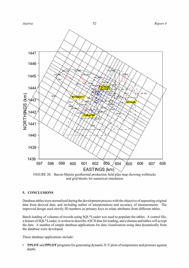
picture of the temperature and pressure distribution at different levels of the reservoir. From contours, ageneral pattern of flow can be inferred and used in assigning the heat source or the outflow crop in thereservoir. To facilitate the creation of contours at different depths of interest, a simple contouring programwas written to access stable temperature, pressure, and well tracks data from the database to make contourmaps (Figures 14-17).

Plots of temperature and pressure areanalyzed to estimate the stableformation temperature and pressure.Relevant portions of temperature andpressure surveys are chosen to givea best approximation of formationtemperature into an estimatedtemperature profile which is plottedagainst elevation. Temperature andpressure points, selected by reservoirengineers to establish a stable wellprofile, are inputted into the Oracledatabase.

The polynomial equations describingthese stable temperature and pressureprofiles are also loaded into theOracle database. Polynomialequations are used to allow

interpolation between points of the log where there is no data. Such is the case when a mechanical gaugeis used for logging, resulting in gaps in the logged depths. Polynomial equations for stable temperatureand pressure, in conjunction with polynomial equations describing the track of vertical and deviated wells,are used to obtain welltrack coordinates and temperature and pressure values at any given depth. In turn,these estimated stable temperature and pressure values are used to generate contours.

A simple contouring program called CONTOUR was developed to retrieve data from the database and

Report 4 Austria49




generate dynamic contour plots. Theprogram basically has two majorparts: data retrieval and data display.The first part is an embedded SQL+script in UNIX which is used toselect welltrack coordinates,temperature, and pressure values forany project location at any depth ofinterest from the table of polynomialequations and generate an input filenamed xyztemp.

The second part is a GMTmanipulation kshell script that isused to generate contours. Thekshell script looks for the input filexyztemp, grids the input file, andcontours the gridded file. The scriptalso sets the color scheme, puts onthe name of the wells, and the valuesof prominent contour lines. Theprogram CONTOUR can createtemperature and pressure distributionfor any project location at any givendepth. The script for the program isshown in Appendix V.

Like TPLOT and PPLOT X-Yplotting programs, the CONTOURprogram can display dynamic data.Any changes made on the data usingthe forms editor or SQL+ commandsare automatically reflected in thecontour plots. The program is veryscalable, in the sense that, anyreservoir parameter can be contouredby updating the Select statement inthe program code to select otherreservoir parameters.

The program CONTOUR is used tocreate temperature contours atdifferent elevations for the Bacon-Manito geothermal production field.These contours can be improvedfurther by masking areas where thereare no wells and therefore notemperature data, and by includingthe complete tracks of wells insteadof only the point in the track of thewell at the given elevation (seeFigures 14 to 17).

To run the program, the user isprompted to enter the ID of the

Austria Report 450

X

A'

Ref. Pt. (E0, N0)

Data Pt. (E1, N1)

Cutting lin

e

A

Well track

aA'

(E0, N0)

(E1, N1)

Cutting lin

e

Well track

X sin β

X cos β

∆E = E1 - E0

-N = N1 - N0

a

b

β

β

X

b

sin

costanNX

XE∆−

−∆=

βββ

ββββ costansintan XENX −∆=∆−

βββ

ββ cos

cossin

cossin 2

XENX−∆=∆

−

ββββ 22 coscossinsin XENX −∆=∆−

geothermal project and the depth where the contour is to be generated. The program usage is describedin the lines below:

Program T – C O N T O U R to get Temperature planes from OracleUsage: tcontour project_ID depth_of_interest

The code for this program is listed in Appendix VI.

4.6 Scripts to generate data file for vertical slice

After creating surface contours, temperature of the wells at different elevations can be used to createvertical sections. Temperature and pressure can be projected at a given cross-sectional cut to generate avertical section. A SQL+ script is written to select the data points to plot well tracks and contours in avertical slice. The same SQL+ script used in program CONTOUR is used to get easting, northing, andtemperature data. Then a simple triangulation procedure is used to project these data points to a cuttingplane from a reference point (see Figures 18a and 18b).

FIGURE 18: a) Surface map; b) Solution by similar triangles

The procedure below describes the calculation procedure in computing the projected distance, X, to thecutting plane.

(1)

Transposing Equation 1 gives:

(2)

Equation 2 can also be expressed as:

(3)

Multiplying both sides of Equation 3 by cos $ :

(4)

When similar terms are grouped, Equation 4 becomes:

Report 4 Austria51

ββββ sincos)cos(sin 22 NEX ∆+∆=+

ββ sincos NEX ∆+∆=

βsin)N(N)cosβE(EX 0101 −+−=

-2500

-2000

-1500

-1000

-500

0

500

DEP

TH, m

RSL

IM-1

PAL-1RD

PAL-3RD

PAL-1

PAL-6D OP-1RD

OP-3DOP-4D

PAL-14D

PAL-8D

PAL-12D

PAL-11D

PAL-18D

PAL-7D

PAL-10D

UPFLOW

STEAM CAP

INANG-MAHARANG

SURFACEDISCHARGES

PALAYAN-BAYANREINJECTION

SECTORBOTONG

LAYER 1

LAYER 2

LAYER 3

LAYER 4

LAYER 5

LAYER 6

220240

180 140

220

240220 280

260

140

280

24026 0300

220260240180

FIGURE 19: Bacon-Manito geothermal production field vertical section showingtemperature contours, welltracks, upflow and outflow areas, grid layers,

and centres of layers for numerical simulation

(5)

However, sin2 $ + cos2 $ = 1. Hence Equation 5 becomes:

(6)

where )E = E1 - Eo and )N = N1 - No.

When these definitions are used in Equation 6, then it becomes:

(7)

Equation 7 can be embedded in a SQL+ script to project the welltracks and temperature of all the wellsin a given geothermal field to a given cross-sectional plane, and create a vertical section. Vertical cross-sections of temperature and pressure are very useful in analyzing the fluid movement in the reservoir andin making a conceptual model of the reservoir. Figure 19 shows how a vertical section is used to visualizethe direction of fluid flow in the reservoir.

4.7 Mesh creation for numerical simulation

Modelling constitutes the most powerful tool available to the reservoir engineer, and is applied to variousmanagement purposes. Modelling needs lots of data and in this regard, mathematical models aredeveloped on the basis of the historical data stored in the Oracle database, and data visualization tools.Through modelling, the nature and properties of the system can be estimated and its behaviour understood.

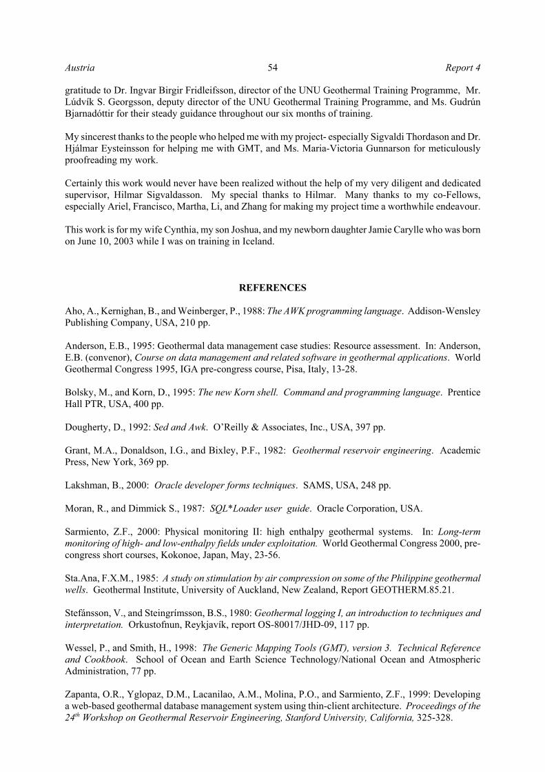
The mesh grid shown in Figure 20 is produced using Grapher (and a simple macro written in Excel) todraw the grid lines (see Appendix VII). The mesh grid shows the model layer from 1.2 km. to 1.6 km.below sea level. It contains welltracks, coordinates of the well track at this elevation, and the grid blocks.Block properties for the input deck are stored in tables in the Oracle database. These include propertiesof the reservoir rocks and model volume, geometry, and boundary conditions which were interpreted usingdata collected over time from surface exploration, exploration drilling, logging, and well testing.

Austria Report 452

EASTINGS (km)

NO

RTH

ING

S (k

m)

PAL-3RD

PAL-1

PB-1A

OP-2RD

CN-2RD

IM-1

SIH-1 OP-1RD

PAL-5D

PAL-16D

PAL-6DPAL-14D

PAL-20DPAL-11D

PAL-7D

CN-5D

CN-4D

CN-3D

OP-5DA

OP-3D

OP-6DPAL-21

MAN-2

PAL-2RD

CN-1

CN-2D

CN-3RD

PAL-12D PAL-8D

MAN-1

PAL-4RDPAL-18D

PAL-19

PAL-1RD

PAL-2D

PAL-9D

OP-4D

PAL-17D

PAL-4DPAL-19

PAL-3D OP-7D

PAL-13DPAL-15D

PAL-10D

BOTONG

MASAKROT

PALAYANBAYAN

CAWAYAN

597 598 599 600 605602601 603 604 606 607 608

1447

1446

1445

1444

1443

1442

1441

1440

1439

1438

FIGURE 20: Bacon-Manito geothermal production field plan map showing welltracksand grid blocks for numerical simulation

5. CONCLUSIONS

Database tables were normalized during the development process with the objective of separating originaldata from derived data, and including author of interpretations and accuracy of measurements. Theimproved design used strictly ID numbers as primary keys to relate attributes from different tables.

Batch-loading of volumes of records using SQL*Loader was used to populate the tables. A control file,a feature of SQL*Loader, is written to describe ASCII data for loading, and columns and tables will acceptthe data. A number of simple database applications for data visualization using data dynamically fromthe database were developed.

These database applications include:

• TPLOT and PPLOT programs for generating dynamic X-Y plots of temperature and pressure againstdepth;

Report 4 Austria53

• CONTOUR program for generating dynamic temperature and pressure contours at differentelevations;

• TSERIES program for monitoring wellhead pressure, massflow, and enthalpy trends of individualwells;

• Algorithms for projecting temperature, pressure, and well track to a given cross-sectional cut whichis used to generate vertical sections;

• Simple Excel macro program to create a mesh for numerical modelling.

Oracle Developer forms for viewing welltest, temperature, and pressure data were created for graphicalretrieval, review, and modification of data from the database. With these forms, the user does not needto learn how to use SQL+ programming language to retrieve, update, and save changes to the database.

The data visualization programs that were developed are very scalable. The embedded SQL+ statementin these programs can be easily modified for visualization of other reservoir data of interest. Genericmapping packages like GNUPLOT and GMT were used in the program to minimize the amount of codedevelopment.

The database system and applications developed to retrieve data blocks from the Oracle database to createdynamic line graphs and contour planes, Developer forms, and projection algorithms from within a UNIXshell script, are very useful tools in providing a basic graphic representation of a reservoir. With thedatabase system and visualization tools, the interpretation time during data analysis can be increased byreducing wasted time spent in looking for, loading, and editing data.

This project focussed on the development of the database and database applications for data visualizations.The next phase will focus on the integration of data visualization modules developed in this project to theexisting reservoir engineering database of PNOC-EDC; the linkage of reservoir engineering database withother geothermal databases to obtain a more comprehensive collection of data for model conceptua-lization; and the development of more graphical visualization tools possibly using the Windows platform.

DEFINITION OF TERMS

AWK Aho, Kernighan, Weinberger programming languageGMT Generic Mapping ToolsHTML Hypertext Mark-up Language HTTP Hypertext Transfer ProtocolIIS Internet Information ServerLAN Local Area Network PL/SQL Procedural Language / Structured Query LanguageRDBMS Relational Database Management SystemNAMRIA National Mapping and Resource Information AuthoritySQL Structured Query LanguageTCP/IP Transmission Control Protocol / Internet ProtocolWAN Wide Area Network

ACKNOWLEDGEMENTS

I would like to express my gratitude to the government of Iceland, the United Nations GeothermalTraining Programme, and the management of PNOC-Energy Development Corporation for allowing meto participate in the 25th United Nations University Geothermal Training Programme. My heartfelt

Austria Report 454

gratitude to Dr. Ingvar Birgir Fridleifsson, director of the UNU Geothermal Training Programme, Mr.Lúdvík S. Georgsson, deputy director of the UNU Geothermal Training Programme, and Ms. GudrúnBjarnadóttir for their steady guidance throughout our six months of training.

My sincerest thanks to the people who helped me with my project- especially Sigvaldi Thordason and Dr.Hjálmar Eysteinsson for helping me with GMT, and Ms. Maria-Victoria Gunnarson for meticulouslyproofreading my work.

Certainly this work would never have been realized without the help of my very diligent and dedicatedsupervisor, Hilmar Sigvaldasson. My special thanks to Hilmar. Many thanks to my co-Fellows,especially Ariel, Francisco, Martha, Li, and Zhang for making my project time a worthwhile endeavour.

This work is for my wife Cynthia, my son Joshua, and my newborn daughter Jamie Carylle who was bornon June 10, 2003 while I was on training in Iceland.

REFERENCES

Aho, A., Kernighan, B., and Weinberger, P., 1988: The AWK programming language. Addison-WensleyPublishing Company, USA, 210 pp.

Anderson, E.B., 1995: Geothermal data management case studies: Resource assessment. In: Anderson,E.B. (convenor), Course on data management and related software in geothermal applications. WorldGeothermal Congress 1995, IGA pre-congress course, Pisa, Italy, 13-28.

Bolsky, M., and Korn, D., 1995: The new Korn shell. Command and programming language. PrenticeHall PTR, USA, 400 pp.

Dougherty, D., 1992: Sed and Awk. O’Reilly & Associates, Inc., USA, 397 pp.

Grant, M.A., Donaldson, I.G., and Bixley, P.F., 1982: Geothermal reservoir engineering. AcademicPress, New York, 369 pp.

Lakshman, B., 2000: Oracle developer forms techniques. SAMS, USA, 248 pp.

Moran, R., and Dimmick S., 1987: SQL*Loader user guide. Oracle Corporation, USA.

Sarmiento, Z.F., 2000: Physical monitoring II: high enthalpy geothermal systems. In: Long-termmonitoring of high- and low-enthalpy fields under exploitation. World Geothermal Congress 2000, pre-congress short courses, Kokonoe, Japan, May, 23-56.

Sta.Ana, F.X.M., 1985: A study on stimulation by air compression on some of the Philippine geothermalwells. Geothermal Institute, University of Auckland, New Zealand, Report GEOTHERM.85.21.

Stefánsson, V., and Steingrímsson, B.S., 1980: Geothermal logging I, an introduction to techniques andinterpretation. Orkustofnun, Reykjavík, report OS-80017/JHD-09, 117 pp.

Wessel, P., and Smith, H., 1998: The Generic Mapping Tools (GMT), version 3. Technical Referenceand Cookbook. School of Ocean and Earth Science Technology/National Ocean and AtmosphericAdministration, 77 pp.

Zapanta, O.R., Yglopaz, D.M., Lacanilao, A.M., Molina, P.O., and Sarmiento, Z.F., 1999: Developinga web-based geothermal database management system using thin-client architecture. Proceedings of the24th Workshop on Geothermal Reservoir Engineering, Stanford University, California, 325-328.

Report 4 Austria55

APPENDIX I: Data dictionary for PNOC-EDC reservoir engineering databaseTable PROJECT - defines a well location by geographical coordinates of a projectColumn name Description Data type Constraint Remarks

Project project ID N 5 PKProjcode acronym of project name VC 10 Not null BGPF, CLGP, LGPP, MCGP, MGPF, MLGP, MNGP, MPGP, NNGP, SLGP, SNGPAddress mailing address of project VC 50 Sorsogon, SorsogonX X coordinate N 10,1 999999999.9 easting, (m)Y Y coordinate N 10,1 999999999.9 northing, (m)Radius radius of a circular area N 5,1 9999.9 (m)Remarks official name of a geothermal field VC 50 Bacon-Manito Geothermal Production Field, Central Leyte Geothermal Project,

Leyte Geothermal Production Field, Mt. Cagua Geothermal Project, Mt. Apo Geothermal Production Field, Mt. Labo Geothermal Project, Mt. Natib Geothermal Project, Mt. Pinatubo Geothermal Project,Northern Negros Geothermal Project, Southern Leyte Geothermal Prod. Field,Southern Negros Geothermal Production Field

Table SECTOR - defines a well location by geographical coordinates of a sectorColumn name Description Data type Constraint Remarks

Sector sector ID N 5 PK Validate using ProjectProject project ID N 5 FKSectcode sector name VC 10 Alto Peak (AP), Upper Mahiao (UM), Lower Mahiao (LM), etc.X X coordinate, easting N 10,1 999999999.9 easting, (m)Y Y coordinate, northing N 10,1 999999999.9 northing, (m)Radius radius of a circular area N 5,1 9999.9 (m)Remarks general comments about sector area VC 50 Tongonan, Pataan, Palayang Bayan

Table PAD - defines well location by geographical coordinates of a pad areaColumn name Description Data type Constraint Remarks

Pad pad ID N 5 PK Validate using SectorSector sector ID N 5 FKPadcode pad name VC 10 212, MGRD1B, OK8, PALRC, PALRA, 300B, etc.X X coordinate, easting N 10,1 999999999.9 easting, (m)Y Y coordinate, northing N 10,1 999999999.9 northing, (m)Radius radius of a circular area N 5,1 9999.9 (m)Remarks general comments about pad area VC 50

Table CELLAR - defines a well location by geographical coordinates of a cellar Column name Description Data type Constraint Remarks

Cellar cellar ID N 5 PK Validate using PadPad pad ID N 5 FKCellarcode cellar name VC 10 Deep cellar (D), standard cellar (S)X X coordinate, easting N 10,1 999999999.9 easting, (m)Y Y coordinate, northing N 10,1 999999999.9 northing, (m)Radius radius of a circular area N 5,1 9999.9 (m)

Table WELL - defines a well location by geographical coordinates of a wellColumn name Description Data type Constraint Remarks

Well well ID N 10 PKPad pad ID N 5 FK Validate using SectorWellname well name VC 10 101, MN1, MG23D, 4R4D, OP5DAX X coordinate of wellhead, easting N 10,1 999999999.9 easting, (m)Y Y coordinate of wellhead, northing N 10,1 999999999.9 northing, (m)Z elevation of wellhead N 5,1 9999.9 elevation, from sea level (m)Measdepth total measured depth of the well N 5,1 9999.9 (m)Whead wellhead ID N 10, 1 999999999.9 indicate wells drilled on same wellhead but with different tracks

Table DRILLJOB - contains details of a drilling activity done on a well Column name Description Data type Constraint Remarks

Drilljob drilling ID N 5 PKWell well ID N 5 FK Validate using WellActivity type of drilling activity VC 5 New well drilling (NW), sidetrack (ST), tophole (TH), workover (WO),

workover and acidizing (WOA), casing relining (RL), redrill to make new well (RD), reentry (RE), perforation and acidizing (PFA), perforation (PF),hydraulic fracturing (HF), air lifting (AIR), plug and abandon (PA).

Date_start date of start of drilling D Format : mm/dd/yyyyDate_end date of end of drilling D Format : mm/dd/yyyyDepth_start starting depth of drilling activity N 4,1 9999.9Depth_end final depth of drilling activity N 4,1 9999.9Rig name of rig used VC 10 rig 9Purpose reason for doing activity VC 150 to increase reinjection capacity for MahanagdongRkbchf distance from rotary table to wellhead N 4,2 99.1

Table DS - contains results of deviation surveys conducted on a wellColumn name Description Data type Constraint Remarks

Ds directional survey ID N 8 PKWell well ID N 5 FK Validate using WellDsmd directional survey, measured depth N 5,1 9999.9 measured depth, (m)Dsvd directional survey, vertical depth N 5,1 9999.1 vertical depth, (m) Dsmn directional survey, meters northing N 10,1 999999999.9 northing, (m)Dsme directional survey, meters easting N 10,1 999999999.9 easting, (m)Dogleg dogleg severity N 5,1 999999999.9Drift drift angle N 4,2 99.99User_initial id of user who inputted record VC 8 I5108Date_start date of inputting D Format : MM-DD-YYYYUser_change id of user who changed record VC 8 I5108Date_change date of change D Format : MM-DD-YYYY

Austria Report 456

Table COMPLETION - contains completion test results for a wellColumn name Description Data type Constraint Remarks

Completion completion test ID N 5 PKWell well ID N 5 FK Validate using WellDate_start date of start of drilling D Format : mm/dd/yyyyDate_end date of end of drilling D Format : mm/dd/yyyyInjectivity injectivity index N 4,1 999.9 (li/s-Mpa)Injdepth tool setting depth during injection test N 5,1 9999.9 measured depth, (m)Maxwhp maximum whp during injectivity test N 5,2 999.9 (MPag)kh permeability thickness N 8,3 999.99999 (Darcy-meter)Skin skin, positive value shows damage while N 4,1 999.9 5, -10

negative value indicates enhanced permeabilty

Table CASING - contains casing configuration of a wellColumn name Description Data type Constraint Remarks

Casing casing ID N 5 PKDrilljob drilling ID N 5 FK Validate using DrilljobWell well ID N 5 FK Validate using WellCBL sonic log ID N 5 FKDate_start date of start of setting of casing D F : mm/dd/yyyyDate_end date of end of setting of casing D F : mm/dd/yyyyCsgtype type of casing C 2 anchor casing (AC), blank liner (BL), intermediate casing (IC), prod. casing (PC),

surface casing (SC), slotted liner (SL)OD outer diameter N 4,1 999.9 (mm)ID inner diameter N 4,1 999.9 (mm)Top top of casing N 5,1 9999.9 vertical depth, (m)Bottom bottom of casing N 5,1 9999.9 vertical depth, (m)

Table PZ - details on permeable zones of wells delineated from different testsColumn name Description Data type Constraint Remarks

Well well ID N 5 FK Validate using ProjectCompletion completion test ID N 5 FK Validate using CompletionPzfrom payzone interval from N 5,1 9999.9 measured depth, (m)Pzto payzone interval to N 5,1 9999.9 measured depth, (m)Pzcode classification of permeable zone VC 2 major (MJ), minor (MN)Source description of data source VC 3 completion test (CT), electronic-line survey (TP)Remarks description of feedzone VC 30 coincides with Kinabkaban fault

Table WELLSTIM - details on stimulation jobs performed on wellsColumn name Description Data type Constraint Remarks

Wellstim well stimulation ID N 10 PKWell well ID N 5 FK Validate using WellEquiptype type of equipment used VC 12 Bauer, SullairDate_start date of start of stimulation activity D F : mm/dd/yyyyDate_end date of end of stimulation activity D F : mm/dd/yyyyOphrs operating hours N 5, 2 1000.0 time, (hr)Oper id of operator who performed the job VC 25Engr id of engineer who supervised the job VC 25 I5108Maxpress maximum pressure N 4, 1 9999.9 (Mpag)Fuelit fule consumed N 5 99999.0 liters, (l)Remarks general remarks about stimulation job VC 100 well succesfully discharged

Table WELLUSE - details about how a well is utilizedColumn name Description Data type Constraint Remarks

Welluse well use ID N 5 PKWell well ID N 5 FK Validate using WellWelluse current use of the well C 2 production (P), reinjection (RI), monitoring (M), temperature gradient (TG),

exploratory (EX)Wellstat current status of the well C 2 shut (S), flowing (F), on bleed (OB), medium term discharge (MTD),

vertical discharge (VD), workover (WO), plugged and abandoned (PA)heat-up (H)

Date date of well utilization record D Format : mm/dd/yyyyTime time of well utilization record Time 12:30:30 Format : hh:mm:ssWhp wellhead pressure N 4,1 999.9 (MPag)

Table BOM - processed bore output measurement dataColumn name Description Data type Constraint Remarks

Bom bore output measurements id N 10 PKWell well ID N 5 FK Validate using WellDate_start data of start of bore output test D Format : mm/dd/yyyyOpening wellhead condition, back pressure plate series VC 3 fullbore (FB), throtled (THR), BPP series : (A1), (B2), etc.WHP whp during bore output test N 5, 2 999.9 (MPag)Enthalpy computed enthalpy N 4 9999.0 (kJ/kg)Waterf computed waterflow N 4, 1 99.9 (kg/s)Massf computed massflow N 4, 1 99.9 (kg/s)Steamf computed steamflow N 4, 1 99.9 (kg/s)Power computed power N 4, 1 99.9 (MWe)Flag flags measurements used for curves N 2 99 stable (S)

Table LOGF - general information about a logging activityColumn name Description Data type Constraint Remarks

Log log ID N 10 PK Validate using LogWell well ID N 5 FK Validate using WellTool tool id N 5 FK Validate using ToolCondition well condition while survey is being done VC 30 1 day shut; after post acidizing completion test; waterlossDate_start date of start of logging activity D Format : mm/dd/yyyyDate_end date of end of logging activity D Format : mm/dd/yyyyShift shift in depth to correct reference depth N 4,1 999.9 mLogdirection direction of log VC 1 upward (U), downward (D), stationary (S)Engr id of engineer in charge of log VC 25 I5108

Report 4 Austria57

Table DDATA - logging data with respect to depthColumn name Description Data type Constraint Remarks

Log log ID N 10 FK Validate using LogDepth depth of log N 5 9999.9 reduced depth (mRSL)Value value recorded in log N 5, 2 999.99 temperature, (°C); pressure, (MPag)

Table TDATA - logging data with respect to timeColumn name Description Data type Constraint Remarks

Log log ID N 10 FK Validate using LogTime time of measurement Time 12:30:30 Format: hh:mm:ssValue value recorded in log N 5, 2 999.99 temperature, (°C); pressure, (MPag)

BLOCKAGE - Table of blockages detected inside the well during surveys and testsColumn name Description Data type Constraint Remarks

Well well ID N 5 PK Validate using WellLog log ID N10 FK Validate using LogTool tool id C 3 FK Validate using Tool

dummy (DM), Go-devil (GD), Kylen sampler (KA), Kuster temperature (KT),Kuster pressure (KP), lead impression block (LIB), sinker bar (SB), scraper (SC)

Surdate date of survey D Format : mm/dd/yyyyTooldiam outer diameter of tool used in survey N 3,1 99.9 (mm)Mcd maximum clear depth tagged during survey N 5,1 9999.9 measured depth, (m)Status short description of nature of blockage VC 50 calcite, anhydrite, etc.

Table TOOL - information on tools used during loggingColumn name Description Data type Constraint Remarks

Tool tool ID N 8 PKToolname name of the tool VC 8 NOT NULLTooltype type of instrument VC 3 NOT NULL temperature (T), pressure (P), spinner (S), flowmeter (FM),

sonic (VDL, CBL or CET), neutron (N), gamma (G), resistivity (R), caliper (XY or CIC), casing collar locator (CCL), freepoint (FP)

Brand brand name of the tool VC 20Description specifications of tool used VC 40

Table CALIBRATE - results of calibration of instrument used in logging Column name Description Data type Constraint Remarks

Calibrate calibration_ID N 8 PKTool tool_ID N 8 FK Validate using ToolDatecalib date of calibration D Format : mm/dd/yyyyRangemin minimum range of tool after calibration N 4,1 999.9Rangemax maximum range of tool after calibration N 4,1 999.9Reference standard used in calibration VC 20

Table DEFLECT- equations from calibration of instrument used in loggingColumn name Description Data type Constraint Remarks

Calibrate calibration_ID N 5 FKTemp temperature N 5 FKPress pressure DError error

Table REPAIRS - details of repair of instruments used in logging Column name Description Data type Constraint Remarks

Calibrate calibration ID N 5 FK Validate using CalibrateDate date of repair D Format : mm/dd/yyyyResult results of repair VC 50

Table CBL - processed cement bond, variable density, and cement evaluation log informationColumn name Description Data type Constraint Remarks

CBL sonic log ID N 5 PKLog log ID N 5 FK Validate using LogfCBLfrom start of cbl interval (top) N 5,1 9999.9 measured depth, (m)CBLto end of cbl interval (bottom) N 5,1 9999.9 measured depth, (m)Bondpct percent of bond index N 3,1 99.9 (%)

Table TRACKPOLY - contains polynomial equations describing the welltrack of well against reduced depthColumn name Description Data type Constraint Remarks

Well well ID N 5 99999.0 Validate using WellKopmod kick off point, modified to simplify polynomials N 6, 2 10000.0Accuracy accuracy of polynomial equations N 2 99.0 accuracy of 10 means accurate within 10 meters, (m)Date_eqn date of creation of polynomial equations D Format : mm/dd/yyyyMevsrd_0 coef of deg 0 polynomial for easting vs. RD N 10, 2 99999999.99Mevsrd_1 coef of deg 1 polynomial for easting vs. RD N 12, 10 99.9999999999Mevsrd_2 coef of deg 2 polynomial for easting vs. RD N 17, 15 99.9999999999999Mevsrd_3 coef of deg 3 polynomial for easting vs. RD N 19, 17 99.9999999999999Mevsrd_4 coef of deg 4 polynomial for easting vs. RD N 22, 20 99.9999999999999Mnvsrd_0 coef of deg 0 polynomial for northing vs. RD N 10, 2 99999999.99Mnvsrd_1 coef of deg 1 polynomial for northing vs. RD N 11, 9 99.999999999Mnvsrd_2 coef of deg 2 polynomial for northing vs. RD N 16, 14 99.9999999999999Mnvsrd_3 coef of deg 3 polynomial for northing vs. RD N 19, 17 99.9999999999999Mnvsrd_4 coef of deg 4 polynomial for northing vs. RD N 22, 20 99.9999999999999Mmdvsrd_0 coef of deg 0 polynomial for MD vs. RD N 12, 8 9999.99999999Mmdvsrd_1 coef of deg 1 polynomial for MD vs. RD N 11, 9 99.999999999Mmdvsrd_2 coef of deg 2 polynomial for MD vs. RD N 15, 13 99.9999999999999Mvdvsrd_0 coef of deg 0 polynomial for VD vs. RD N 6, 2 9999.99Mvdvsrd_1 coef of deg 1 polynomial for VD vs. RD N 3, 2 9.99Source ID of author of equations VC 10

Note : vertical depth (VD), measured depth (MD), reduced depth (RD)

Austria Report 458

Table STABLETEMP - contains interpreted stable temperatures for wellsColumn name Description Data type Constraint Remarks

Well well ID N 5 99999.0 Validate using Well

Date_int date interpretation was made and inputted todbase D Format : mm/dd/yyyy

Reducedepth reduced depth where temperature is given N 5 99999.0Temperature interpreted stable temperature N 4, 1 9999.9Source ID of author of interpreted temperatures VC 15

Table STABLEPRES - contains interpreted stable pressures for wellsColumn name Description Data type Constraint Remarks

Well well ID N 5 99999.0 Validate using WellDate_int date of interpretation and inputting D Format : mm/dd/yyyyReducedepth reduced depth where pressure is given N 5 99999.0Pressure interpreted stable pressure N 4, 1 9999.9Source ID of author of interpreted pressures VC 15

APPENDIX II: UNIX shell script for temperature plotting program TPLOT

#! /bin/ksh## T P L O T# Year created 2003# Jaime and Hilmar# Script using S Q L + and G N U P L O T © to get Temperature logs # from Oracle tables WELL, DDATA, and LOGF#echo "Program T P L O T to get Temperature logs from Oracle" if [[$# -lt 3 || $1 = "-h”]]thenecho "Usage: tplot wellname fromdate(DD-MM-YYYY) todate(DD-MM-YYYY)" 1>&2 exit 1fiecho "set echo offset feedback offset flush offset term offset verify offset newpage 0set lines 130set pages 0

break on log on notes skip 2

spool tselect distinct a.value, a.depth, b.date_start, b.log, to_char (b.date_start,'DD-MM-YYYY')||'-'||b.condition Notesfrom ddata a, logf b, well cwhere a.log = b.logand b.well = c.welland b.condition = ‘T’and c.wellname = '$1'and b.date_start >=to_date('$2', 'DD-MM-YYYY')and b.date_start<=to_date('$3', 'DD-MM-YYYY')order by b.date_start, b.log, a.depth;spool off

quit" > t.sql

Report 4 Austria59

sqlplus / @t.sql > /dev/null

# uses Sed to remove blank lines sed 's/^ *$//' t.lst > tt.lst# saves changes to temporary file bb.lst and renames bb.lst to t.lst awk 'NR >= 1 {print $1, $2, $3, $4, $5}' tt.lst > ttt.lstmv ttt.lst t.lst

# Create GNUPLOT commands fileecho "set xdataset ydataset title 'Well $1'set yrange [0:3000] reverse set xrange [0:400]set xtics 100set mxtics 2set ytics 200set mytics 2set xlabel 'Temperature (/C)'set ylabel 'Depth (mVD)'set key right bottom outsideset keytitle 'Survey condition'set size ratio 0 1, 1show size" > sk.tp

awk 'BEGIN{printf("plot ");j=0}NF>4 {a[j]=$5;j++}END{for (i=0;i<j-1;i++) {printf("\"t.lst\" index %d:%d title '\''%s'\'' with linespoints,",i,i,a[i])}printf("\"t.lst\" index %d:%d title '\''%s'\'' with linespoints \npause -1",i,i,a[i])}' t.lst >> sk.tpgnuplot sk.tp

APPENDIX III: UNIX shell script for pressure plotting program PPLOT

#! /bin/ksh## P P L O T# Year created 2003# Jaime and Hilmar# Script using S Q L + and G N U P L O T (C) to get Pressure logs from Oracle # from Oracle tables WELL, DDATA, and LOGF#echo "Program P P L O T to get Pressure logs from Oracle" if [[$# -lt 3 || $1 = "-h”]]thenecho "Usage: tplot wellname fromdate(DD-MM-YYYY) todate(DD-MM-YYYY)" 1>&2 exit 1fi

echo "set echo off

Austria Report 460

set feedback offset flush offset term offset verify offset newpage 0set lines 130set pages 0

break on log on notes skip 2

spool pselect distinct a.value, a.depth, b.date_start, b.log, to_char (b.date_start,'DD-MM-YYYY')||'-'||b.condition Notesfrom ddata a, logf b, well cwhere a.log = b.logand b.well = c.welland b.condition = ‘P’and c.wellname = '$1'and b.date_start >=to_date('$2', 'DD-MM-YYYY')and b.date_start<=to_date('$3', 'DD-MM-YYYY')order by b.date_start, b.log, a.depth;spool off

quit" > p.sqlsqlplus / @p.sql > /dev/null

# uses Sed to remove blank lines sed 's/^ *$//' p.lst > pp.lst# saves changes to temporary file bb.lst and renames bb.lst to t.lst awk 'NR >= 1 {print $1, $2, $3, $4, $5}' pp.lst > ppp.lstmv ttt.lst t.lst

# Create GNUPLOT commands fileecho "set xdataset ydataset title 'Well $1'set yrange [0:3000] reverse set xrange [0:400]set xtics 100set mxtics 2set ytics 200set mytics 2set xlabel 'Pressure (MPag)'set ylabel 'Depth (mVD)'set key right bottom outsideset keytitle 'Survey condition'set size ratio 0 1, 1show size" > sk.tp

awk 'BEGIN{printf("plot ");j=0}NF>4 {a[j]=$5;j++}END{for (i=0;i<j-1;i++) {printf("\"p.lst\" index %d:%d title '\''%s'\'' with linespoints,",i,i,a[i])}printf("\"p.lst\" index %d:%d title '\''%s'\'' with linespoints \npause -1",i,i, a[i])}' p.lst >> sk.tpgnuplot sk.tp

Report 4 Austria61

APPENDIX IV: Interpreted stable temperature and pressure and corresponding polynomial fits of wells in Bacon-Manito geothermal production field

Austria Report 462

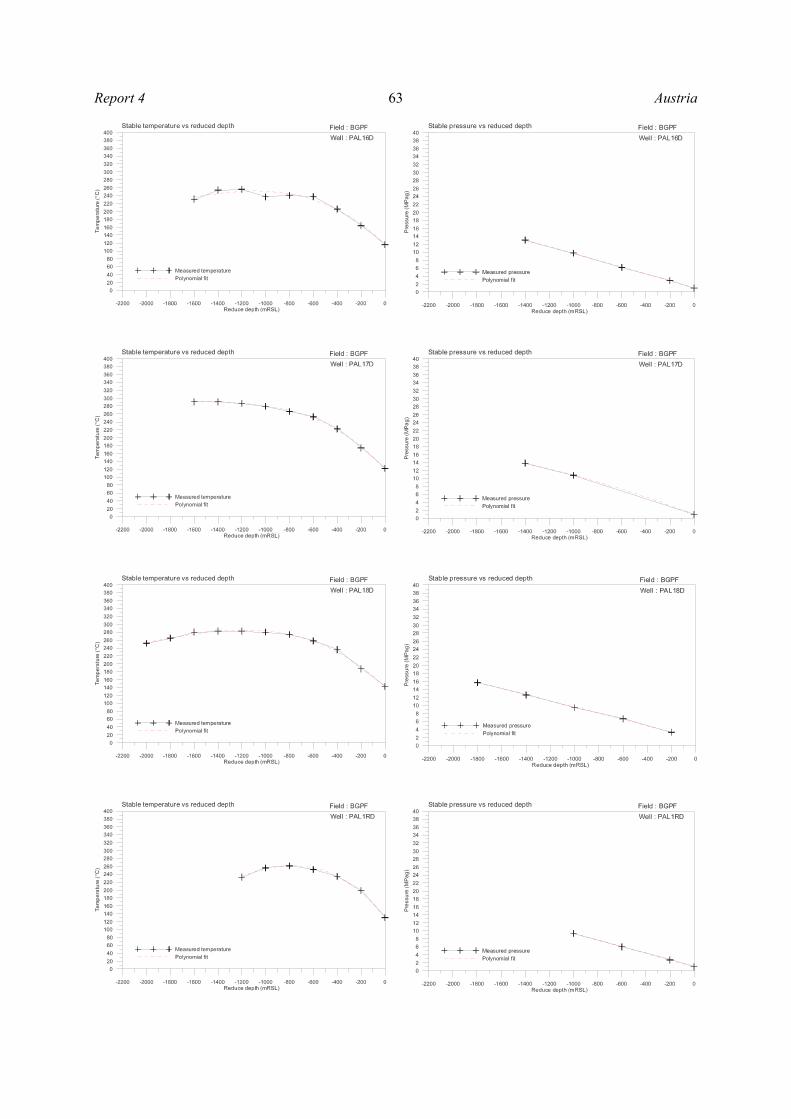
Report 4 Austria63

Austria Report 464

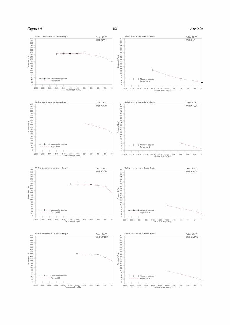
Report 4 Austria65

Austria Report 466

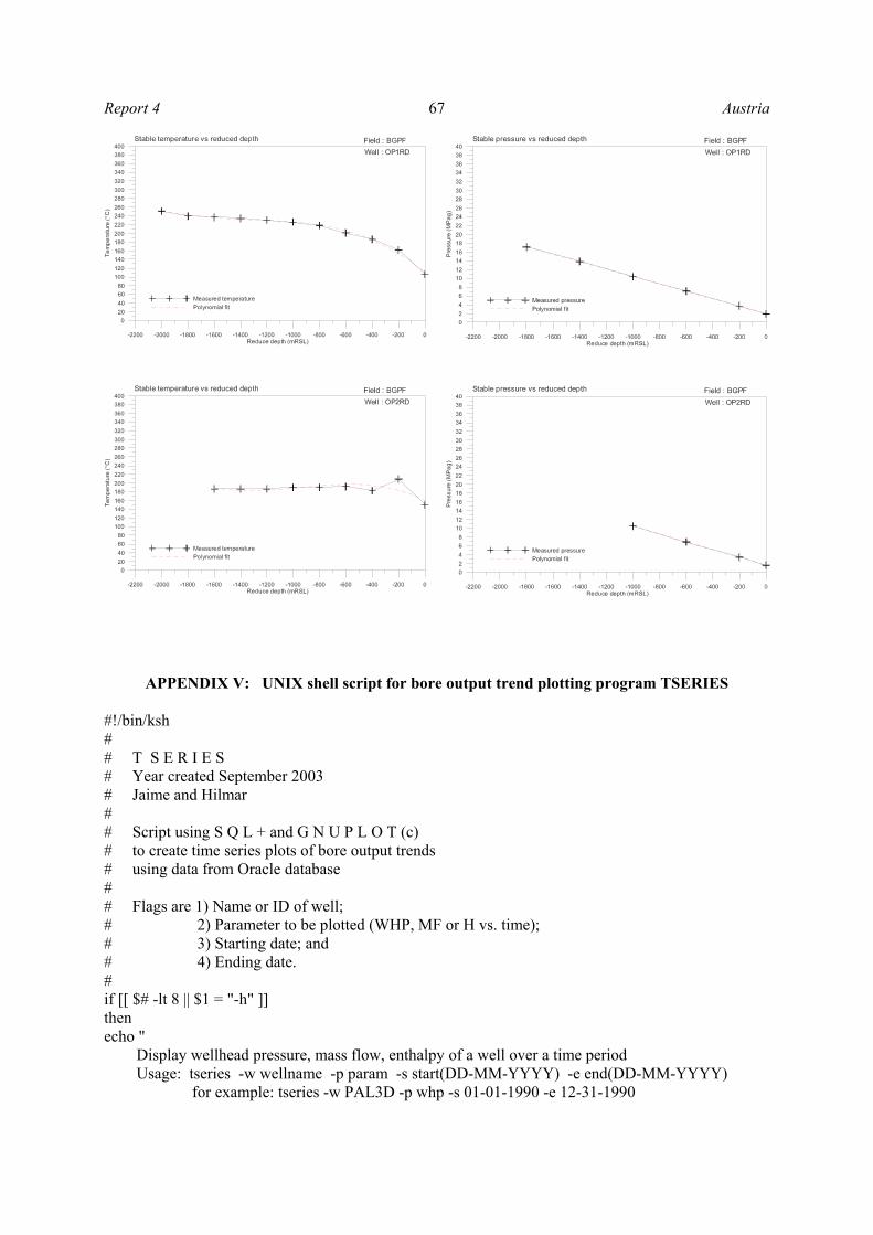
Report 4 Austria67

APPENDIX V: UNIX shell script for bore output trend plotting program TSERIES

#!/bin/ksh## T S E R I E S# Year created September 2003# Jaime and Hilmar## Script using S Q L + and G N U P L O T (c) # to create time series plots of bore output trends# using data from Oracle database## Flags are 1) Name or ID of well;# 2) Parameter to be plotted (WHP, MF or H vs. time);# 3) Starting date; and # 4) Ending date. #if [[ $# -lt 8 || $1 = "-h" ]]thenecho " Display wellhead pressure, mass flow, enthalpy of a well over a time period Usage: tseries -w wellname -p param -s start(DD-MM-YYYY) -e end(DD-MM-YYYY)

for example: tseries -w PAL3D -p whp -s 01-01-1990 -e 12-31-1990

Austria Report 468

PARAMETER -p:whp : Wellhead pressuremf : Massflowh : Enthalpy

OPTIONS -w : wellname -s : starting date -e : ending date" 1>&2 exit 1fi

# Optionsset -- $(getopt "w:p:s:e:" "$@")for arg in $@docase $arg in -w) wellname=$2 shift 2;; -p) parameter=$2 shift 2;; -s) startdate=$2 shift 2;; -e) enddate=$2 shift 2;; --) shift; break;;esacdone

echo Parameters $wellname $parameter $startdate $enddate

# Submenu: wellhead pressure if test $parameter = "whp"thenecho "set echo offset feedback offset flush offset term offset verify offset newpage 0set lines 80set pages 0

spool bore_outputselect a.date_start, a.whpfrom bom a, well b where a.well = b.welland b.wellname = '$wellname' and a.date_start >= '$startdate'and a.date_start <= '$enddate'order by a.date_start;spool offquit" > run.sql

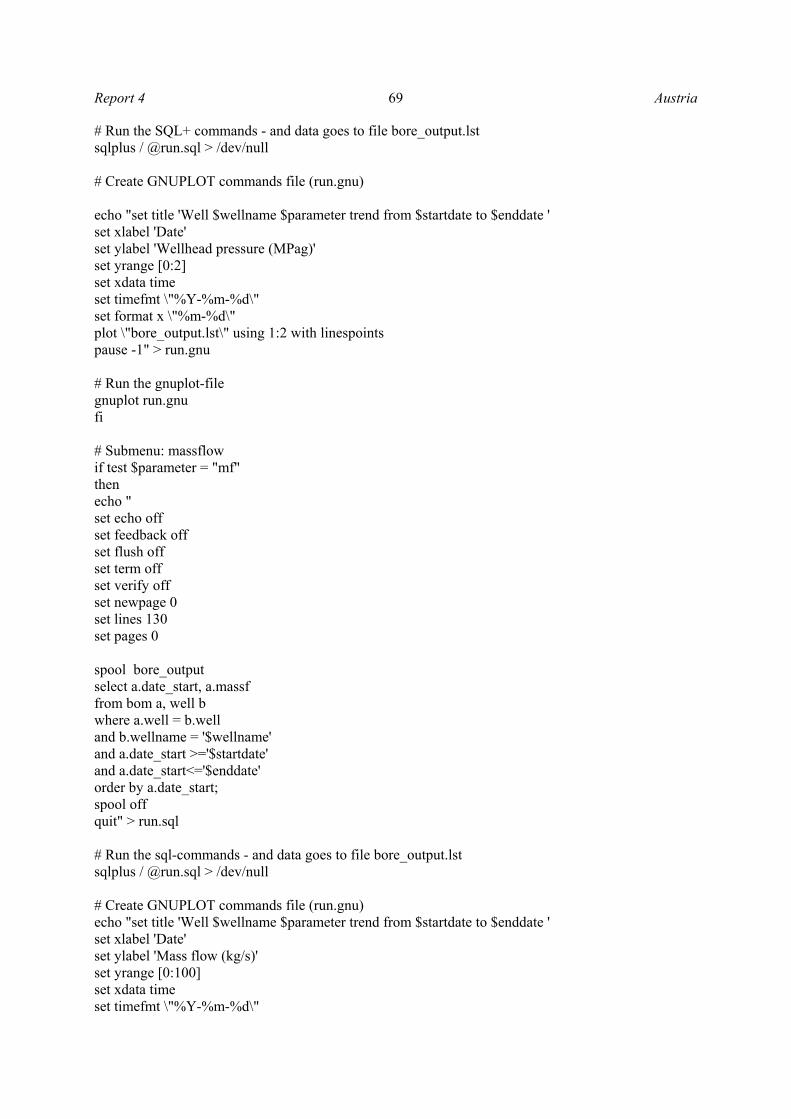
Report 4 Austria69

# Run the SQL+ commands - and data goes to file bore_output.lstsqlplus / @run.sql > /dev/null

# Create GNUPLOT commands file (run.gnu)

echo "set title 'Well $wellname $parameter trend from $startdate to $enddate 'set xlabel 'Date'set ylabel 'Wellhead pressure (MPag)'set yrange [0:2]set xdata timeset timefmt \"%Y-%m-%d\"set format x \"%m-%d\"plot \"bore_output.lst\" using 1:2 with linespointspause -1" > run.gnu

# Run the gnuplot-filegnuplot run.gnufi

# Submenu: massflow if test $parameter = "mf"thenecho "set echo offset feedback offset flush offset term offset verify offset newpage 0set lines 130set pages 0

spool bore_outputselect a.date_start, a.massffrom bom a, well b where a.well = b.welland b.wellname = '$wellname' and a.date_start >='$startdate'and a.date_start<='$enddate'order by a.date_start;spool offquit" > run.sql

# Run the sql-commands - and data goes to file bore_output.lstsqlplus / @run.sql > /dev/null

# Create GNUPLOT commands file (run.gnu)echo "set title 'Well $wellname $parameter trend from $startdate to $enddate 'set xlabel 'Date'set ylabel 'Mass flow (kg/s)'set yrange [0:100]set xdata timeset timefmt \"%Y-%m-%d\"

Austria Report 470

set format x \"%m-%d\"plot \"bore_output.lst\" using 1:2 with linespointspause -1" > run.gnu


# Submenu: enthalpy if test $parameter = "h"thenecho "set echo offset feedback offset flush offset term offset verify offset newpage 0set lines 130set pages 0

spool bore_outputselect a.date_start, a.enthalpyfrom bom a, well b where a.well = b.welland b.wellname = '$wellname' and a.date_start >='$startdate'and a.date_start<='$enddate'order by a.date_start;spool offquit" > run.sql

# Run the sql-commands - and data goes to file bore_output.lstsqlplus / @run.sql > /dev/null

# Create gnuplot-commands file (run.gnu)echo "set title 'Well $wellname $parameter trend from $startdate to $enddate 'set xlabel 'Date'set ylabel 'Enthalpy (kJ/kJ)'set yrange [0:2000]set xdata timeset timefmt \"%Y-%m-%d\"set format x \"%m-%d\"plot \"bore_output.lst\" using 1:2 with linespointspause -1" > run.gnu


Report 4 Austria71

APPENDIX VI: UNIX shell script for temperature contouring program CONTOUR

#!/bin/ksh# # CONTOUR# Year created 2003# Hilmar and Jaime# Script using S Q L + and G M T © to generate input for contouring application# echo "Function XYZ to generate input deck for contouring application" if [[ $# -lt 2 || $1 = "-h" ]]thenecho "Usage: contour Project_ID Depth (mrsl) " 1>&2

exit 1fi

# Gets kick off point (kop)echo "set echo offset feedback offset flush offset term offset verify offset newpage 0set lines 80set pages 0column kop format 999.9

spool kopselect distinct a.well, a.kopmodfrom ops\$jaja.trackpoly a, ops\$jaja.wellbyproj bwhere a.well = b.welland b.project = '$1';spool off

quit" > j1.sqlsqlplus / @j1.sql > /dev/null

# Gets (wellname, easting, northing, vertical depth, temperature) for all vertical wellsecho "set echo offset feedback offset flush offset term offset verify offset newpage 0set lines 80set pages 0column easting format 9999999column northing format 99999999column vertical format 9999.9

Austria Report 472

column measured format 9999.9column temperature format 9999spool xyztemp" > j2.sql

awk 'BEGIN{printf("select a.wellname, a.x easting, a.y northing, a.z - %d vertical, \n",'$2');printf("( b.stemp_0 + b.stemp_1 * power((%5.1f),1) + b.stemp_2 * power((%5.1f),2) + b.stemp_3 *power((%5.1f),3) + b.stemp_4 * power((%5.1f),4) ) temperature \n", '$2','$2','$2','$2');printf("from ops$jaja.well a, ops$jaja.stabletempeqn b\nwhere a.well = b.well\nand a.well in (\n")}$2 <= '$2' {well[j] = $1;j++}END {for (i = 1;i<j-1;i++) {printf("%d,\n",well[i])}printf("%d)\n;\n",well[j-1])}' kop.lst >> j2.sql

# Gets (wellname, easting, northing, vertical depth, temperature, measured depth) for deviated wells

awk 'BEGIN {printf("select b.wellname, (a.mevsrd_0 +a.mevsrd_1 * power ((%5.1f), 1) + a.mevsrd_2* power ((%5.1f), 2) + a.mevsrd_3 * power ((%5.1f), 3) + a.mevsrd_4 * power ((%5.1f), 4))easting,\n",'$2','$2','$2','$2');printf("(a.mnvsrd_0 * power ((%5.1f), 0) + a.mnvsrd_1 * power ((%5.1f), 1) + a.mnvsrd_2 * power((%5.1f), 2) + a.mnvsrd_3 * power ((%5.1f), 3) + a.mnvsrd_4 * power ((%5.1f), 4)) northing,\n",'$2','$2','$2','$2','$2');printf("(a.mvdvsrd_0 * power ((%5.1f), 0) +a.mvdvsrd_1 * power ((%5.1f), 1)) vertical, \n", '$2', '$2');printf("( c.stemp_0 + c.stemp_1 * power((%5.1f),1) + c.stemp_2 * power((%5.1f),2) + c.stemp_3 *power((%5.1f),3) + c.stemp_4 * power((%5.1f),4) ) temperature, \n", '$2','$2','$2','$2');printf("(a.mmdvsrd_0 * power ((%5.1f), 0) + a.mmdvsrd_1 * power ((%5.1f), 1) + a.mmdvsrd_2 *power ((%5.1f), 2) ) measured \n",'$2','$2','$2');printf("from ops$jaja.trackpoly a, ops$jaja.WELL b, ops$jaja.stabletempeqn c\nwhere a.well =c.well\nand a.well = b.well\nand c.well in (\n")}$2 > '$2' {well[j] = $1;j++}END {for (i=1; i< j-1;i++) {printf("%d,\n",well[i])}printf("%d)\n;\n",well[j-1])}' kop.lst >> j2.sqlecho "spool off

quit" >> j2.sqlsqlplus / @j2.sql > /dev/null

# Deletes data rows with negative temperature and vertical depth # Prints (easting, northing, temperature, wellname)awk '$4 > 0 {print $2,$3, $5, $1}' xyztemp.lst > xyztemp

# GMT part

GMT_HOME=/usr/local/apps/GMT3.4/bin$GMT_HOME/gmtset LABEL_FONT_SIZE 11 ANOT_FONT_SIZE 10 UNIX_TIME_POS -1/-1.3

# Set limits of x and y for better appearance; instead GMT program minmax gives min/max values:x1=598100 x2=605000 y1=1440100 y2=1445100# Sets data file sourcedatafile=xyztemp# Sets output filepsout=test.ps

rm .gmtcommands# command for initiating projection$GMT_HOME/psbasemap -JX14/10c -R$x1/$x2/$y1/$y2 -Ba1000f1000:"Eastings(m)":/a1000f1000:"Northings (m)"::.$head:SWne -X5 -Y5 -P -K > $psout

Report 4 Austria73

# color ramp for the temperature, always the same# Tin R G B Tfin R G B#echo "-40 40 0 150 110 40 0 150110 0 10 200 160 0 10 200160 0 40 224 180 0 40 224180 13 129 248 190 13 129 248190 50 190 255 200 50 190 255200 97 225 240 210 97 225 240210 124 235 200 220 124 235 200220 172 245 168 230 172 245 168230 223 245 141 240 223 245 141240 247 215 104 250 247 215 104250 255 160 69 260 255 160 69260 238 80 78 270 238 80 78270 255 124 124 280 255 124 124280 245 179 174 290 245 179 174290 255 215 215 300 255 215 215300 255 225 225 310 255 225 225310 255 235 235 320 255 235 235320 255 245 245 330 255 245 245330 255 255 255 360 255 255 255" > color.palette

awk '{print $1,$2,$3}' $datafile | $GMT_HOME/blockmean -I0.5/0.1 -R | surface -Gtmp.grd -I100 -R-T0.3

$GMT_HOME/grdimage tmp.grd -JX -R -Ccolor.palette -O -K -Y >> $psout$GMT_HOME/grdcontour tmp.grd -JX -R -W4 -C10 -Wc2 -A20 -Wa4 -O -K >> $psout

# Plot locations with symbols and textawk '{print $1,$2}' $datafile | $GMT_HOME/psxy -JX -R -Ss0.2 -O -K >> $psout# Add well names to plotawk '{print $1,$2,8,0,1,7,$4}' $datafile | $GMT_HOME/pstext -JX -R -N -O -K >> $psout# adding parameters to plotawk '{print $1,$2,8,0,2,7,$3}' $datafile | $GMT_HOME/pstext -JX -R -N -O >> $psout# display surfacegv $psout &# clean up rm -r kop.lst j1.sql j2.sql xyztemp xyztemp.lst tmp.grd color.palette# Comments: In the PATH variable this directory -> /usr/local/apps/gmt/bin# was used to run the GMT-commands which gave us version 3.0 I think# By declaring GMT_HOME=/usr/local/apps/GMT3.4/bin we are using the version 3.4.3 # This makes a big difference and now we can use the on-line help on the web

Austria Report 474

APPENDIX VII: The Excel macro spreadsheet used to create the grid files

Documents

DATABASE SYSTEM AND APPLICATIONS DEVELOPED FOR RESERVOIR ... · DATABASE SYSTEM AND APPLICATIONS DEVELOPED FOR RESERVOIR ... Energy Development Corporation for reservoir engineering