Embed Size (px)
Citation preview

DatabasescoursebookVersion 4.1(24September2014)FreeUniversityofBolzano Bozen– PaoloColetti
IntroductionThis book contains the relational databases and Access course’s lessons held at the Free University of Bolzano Bozen. The book is divided into levels, the level is indicated between parentheses after each section’s title:
students of Information Systems and Data Management 27000 course use level 1;
students of Information Systems and Data Management 27006 course use levels 1, 2 and 3;
students of Computer Science and Information Processing course use levels 1, 2 and 3;
students of Advanced Data Analysis course use levels 2 and 5.
This book refers to Microsoft Access 2010, with referrals to 2007 and 2003 in footnotes, to MySQL Community Server version 5.5 and to HeidiSQL version 7.0.0.
This book is in continuous development, please take a look at its version number, which marks important changes.
Disclaimers
This book is designed for novice database designers. It contains simplifications of theory and many technical details are purposely omitted.
TableofContentsINTRODUCTION ....................................................... 1
TABLE OF CONTENTS ................................................ 1
1. RELATIONAL DATABASES (LEVEL 2) .................. 2
1.1. DATABASE IN NORMAL FORM ............................ 2 1.2. RELATIONS .................................................... 3 1.3. ONE‐TO‐MANY RELATION ................................. 5 1.4. ONE‐TO‐ONE RELATION .................................... 6 1.5. MANY‐TO‐MANY RELATION ............................... 7 1.6. FOREIGN KEY WITH SEVERAL RELATIONS ............... 9 1.7. REFERENTIAL INTEGRITY ................................. 10 1.8. TEMPORAL VERSUS STATIC DATABASE ................ 11 1.9. NON‐RELATIONAL STRUCTURES ........................ 11 1.10. ENTITY‐RELATIONSHIP MODEL (LEVEL 9) ............ 12
2. MICROSOFT ACCESS (LEVEL 1) ........................ 14
2.1. BASIC OPERATIONS ........................................ 14 2.2. TABLES (LEVEL 1) .......................................... 15 2.3. FORMS (LEVEL 3) .......................................... 18 2.4. QUERIES (LEVEL 1) ........................................ 19
2.5. REPORTS (LEVEL 3) ....................................... 22 3. MYSQL (LEVEL 5) ............................................ 23
3.1. HEIDISQL ................................................... 23 3.2. INSTALLING MYSQL SERVER ........................... 25
4. SQL LANGUAGE FOR MYSQL (LEVEL 5) ............ 29
4.1. BASIC OPERATIONS ....................................... 29 4.2. SIMPLE SELECTION QUERIES ............................ 29 4.3. INNER JOINS ................................................ 31 4.4. SUMMARY QUERIES ...................................... 33 4.5. MODIFYING RECORDS .................................... 34 4.6. EXTERNAL DATA ........................................... 34 4.7. TABLES ....................................................... 35
5. DESIGNING A DATABASE (LEVEL 2) ................. 38
5.1. PAPER DIAGRAM .......................................... 38 5.2. BUILDING THE TABLES .................................... 39 5.3. INSERTING DATA ........................................... 41
6. TECHNICAL DOCUMENTATION (LEVEL 9) ........ 42
6.1. MYFARM EXAMPLE ....................................... 42
Paolo Coletti Databases course book
Page 2 of 44 Version 4.1 (24/09/2014)
1. Relationaldatabases(level2)
This chapter presents the basic ideas and motivations which lie behind the concept of relational database. Readers with previous experience in building schemas for relational databases can skip this part.
A relational database is defined as a collection of tables connected via relations. It is always a good idea to have this table organized in a structured was that is called normal form.
1.1. DatabaseinNormalForm
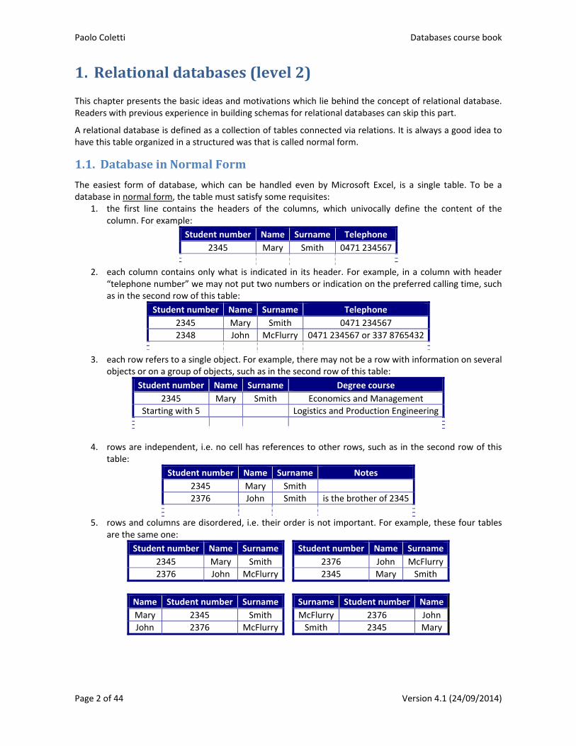
The easiest form of database, which can be handled even by Microsoft Excel, is a single table. To be a database in normal form, the table must satisfy some requisites:
1. the first line contains the headers of the columns, which univocally define the content of the column. For example:
Student number Name Surname Telephone
2345 Mary Smith 0471 234567
2. each column contains only what is indicated in its header. For example, in a column with header
“telephone number” we may not put two numbers or indication on the preferred calling time, such as in the second row of this table:
Student number Name Surname Telephone
2345 Mary Smith 0471 234567
2348 John McFlurry 0471 234567 or 337 8765432
3. each row refers to a single object. For example, there may not be a row with information on several
objects or on a group of objects, such as in the second row of this table:
Student number Name Surname Degree course
2345 Mary Smith Economics and Management
Starting with 5 Logistics and Production Engineering
4. rows are independent, i.e. no cell has references to other rows, such as in the second row of this table:
Student number Name Surname Notes
2345 Mary Smith
2376 John Smith is the brother of 2345
5. rows and columns are disordered, i.e. their order is not important. For example, these four tables
are the same one:
Student number Name Surname Student number Name Surname
2345 Mary Smith 2376 John McFlurry
2376 John McFlurry 2345 Mary Smith
Name Student number Surname Surname Student number Name
Mary 2345 Smith McFlurry 2376 John
John 2376 McFlurry Smith 2345 Mary
Databases course book Paolo Coletti
Version 4.1 (24/09/2014) Page 3 of 44
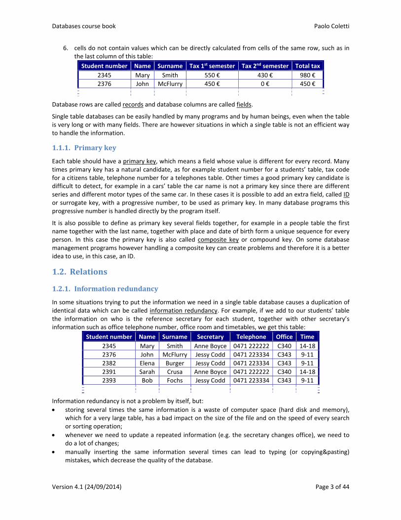
6. cells do not contain values which can be directly calculated from cells of the same row, such as in the last column of this table:
Student number Name Surname Tax 1st semester Tax 2nd semester Total tax
2345 Mary Smith 550 € 430 € 980 €
2376 John McFlurry 450 € 0 € 450 €
Database rows are called records and database columns are called fields.
Single table databases can be easily handled by many programs and by human beings, even when the table is very long or with many fields. There are however situations in which a single table is not an efficient way to handle the information.
1.1.1. Primarykey
Each table should have a primary key, which means a field whose value is different for every record. Many times primary key has a natural candidate, as for example student number for a students’ table, tax code for a citizens table, telephone number for a telephones table. Other times a good primary key candidate is difficult to detect, for example in a cars’ table the car name is not a primary key since there are different series and different motor types of the same car. In these cases it is possible to add an extra field, called ID or surrogate key, with a progressive number, to be used as primary key. In many database programs this progressive number is handled directly by the program itself.
It is also possible to define as primary key several fields together, for example in a people table the first name together with the last name, together with place and date of birth form a unique sequence for every person. In this case the primary key is also called composite key or compound key. On some database management programs however handling a composite key can create problems and therefore it is a better idea to use, in this case, an ID.
1.2. Relations
1.2.1. Informationredundancy
In some situations trying to put the information we need in a single table database causes a duplication of identical data which can be called information redundancy. For example, if we add to our students’ table the information on who is the reference secretary for each student, together with other secretary’s information such as office telephone number, office room and timetables, we get this table:
Student number Name Surname Secretary Telephone Office Time
2345 Mary Smith Anne Boyce 0471 222222 C340 14‐18
2376 John McFlurry Jessy Codd 0471 223334 C343 9‐11
2382 Elena Burger Jessy Codd 0471 223334 C343 9‐11
2391 Sarah Crusa Anne Boyce 0471 222222 C340 14‐18
2393 Bob Fochs Jessy Codd 0471 223334 C343 9‐11
Information redundancy is not a problem by itself, but:
storing several times the same information is a waste of computer space (hard disk and memory), which for a very large table, has a bad impact on the size of the file and on the speed of every search or sorting operation;
whenever we need to update a repeated information (e.g. the secretary changes office), we need to do a lot of changes;
manually inserting the same information several times can lead to typing (or copying&pasting) mistakes, which decrease the quality of the database.
Paolo Coletti Databases course book
Page 4 of 44 Version 4.1 (24/09/2014)
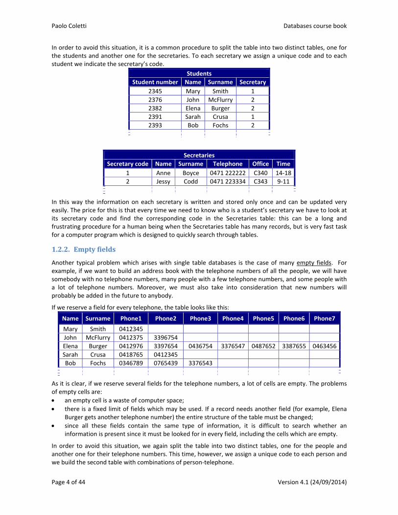
In order to avoid this situation, it is a common procedure to split the table into two distinct tables, one for the students and another one for the secretaries. To each secretary we assign a unique code and to each student we indicate the secretary’s code.
Students
Student number Name Surname Secretary
2345 Mary Smith 1
2376 John McFlurry 2
2382 Elena Burger 2
2391 Sarah Crusa 1
2393 Bob Fochs 2
Secretaries
Secretary code Name Surname Telephone Office Time
1 Anne Boyce 0471 222222 C340 14‐18
2 Jessy Codd 0471 223334 C343 9‐11
In this way the information on each secretary is written and stored only once and can be updated very easily. The price for this is that every time we need to know who is a student’s secretary we have to look at its secretary code and find the corresponding code in the Secretaries table: this can be a long and frustrating procedure for a human being when the Secretaries table has many records, but is very fast task for a computer program which is designed to quickly search through tables.
1.2.2. Emptyfields
Another typical problem which arises with single table databases is the case of many empty fields. For example, if we want to build an address book with the telephone numbers of all the people, we will have somebody with no telephone numbers, many people with a few telephone numbers, and some people with a lot of telephone numbers. Moreover, we must also take into consideration that new numbers will probably be added in the future to anybody.
If we reserve a field for every telephone, the table looks like this:
Name Surname Phone1 Phone2 Phone3 Phone4 Phone5 Phone6 Phone7
Mary Smith 0412345
John McFlurry 0412375 3396754
Elena Burger 0412976 3397654 0436754 3376547 0487652 3387655 0463456
Sarah Crusa 0418765 0412345
Bob Fochs 0346789 0765439 3376543
As it is clear, if we reserve several fields for the telephone numbers, a lot of cells are empty. The problems of empty cells are:
an empty cell is a waste of computer space;
there is a fixed limit of fields which may be used. If a record needs another field (for example, Elena Burger gets another telephone number) the entire structure of the table must be changed;
since all these fields contain the same type of information, it is difficult to search whether an information is present since it must be looked for in every field, including the cells which are empty.
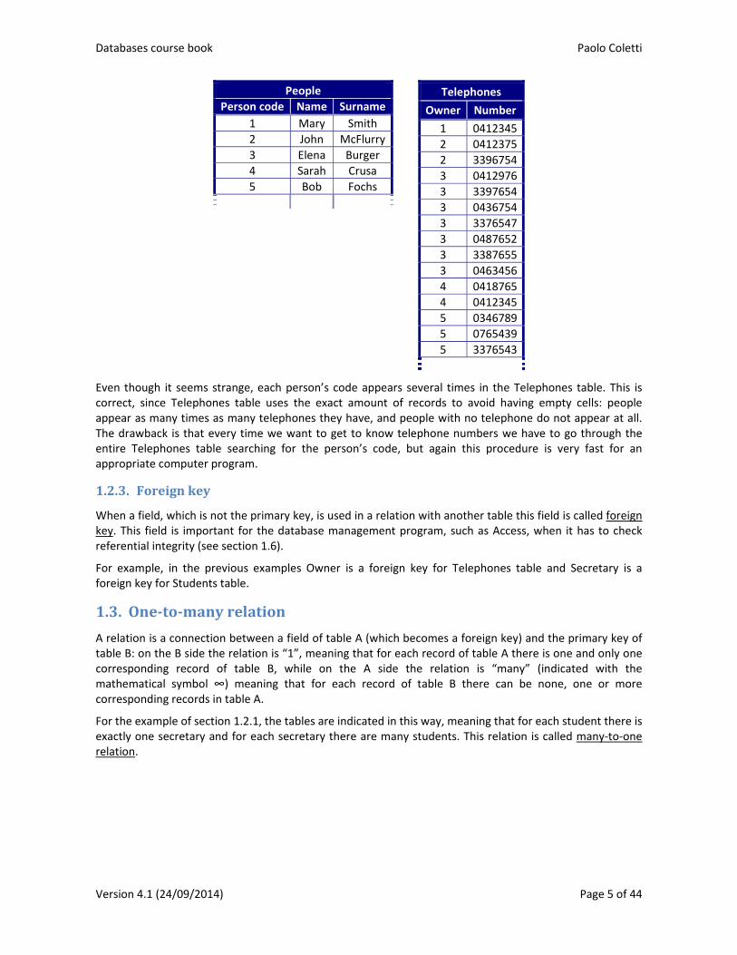
In order to avoid this situation, we again split the table into two distinct tables, one for the people and another one for their telephone numbers. This time, however, we assign a unique code to each person and we build the second table with combinations of person‐telephone.
Databases course book Paolo Coletti
Version 4.1 (24/09/2014) Page 5 of 44
People
Person code Name Surname
1 Mary Smith
2 John McFlurry
3 Elena Burger
4 Sarah Crusa
5 Bob Fochs
Telephones
Owner Number
1 0412345
2 0412375
2 3396754
3 0412976
3 3397654
3 0436754
3 3376547
3 0487652
3 3387655
3 0463456
4 0418765
4 0412345
5 0346789
5 0765439
5 3376543
Even though it seems strange, each person’s code appears several times in the Telephones table. This is correct, since Telephones table uses the exact amount of records to avoid having empty cells: people appear as many times as many telephones they have, and people with no telephone do not appear at all. The drawback is that every time we want to get to know telephone numbers we have to go through the entire Telephones table searching for the person’s code, but again this procedure is very fast for an appropriate computer program.
1.2.3. Foreignkey
When a field, which is not the primary key, is used in a relation with another table this field is called foreign key. This field is important for the database management program, such as Access, when it has to check referential integrity (see section 1.6).
For example, in the previous examples Owner is a foreign key for Telephones table and Secretary is a foreign key for Students table.
1.3. One‐to‐manyrelation
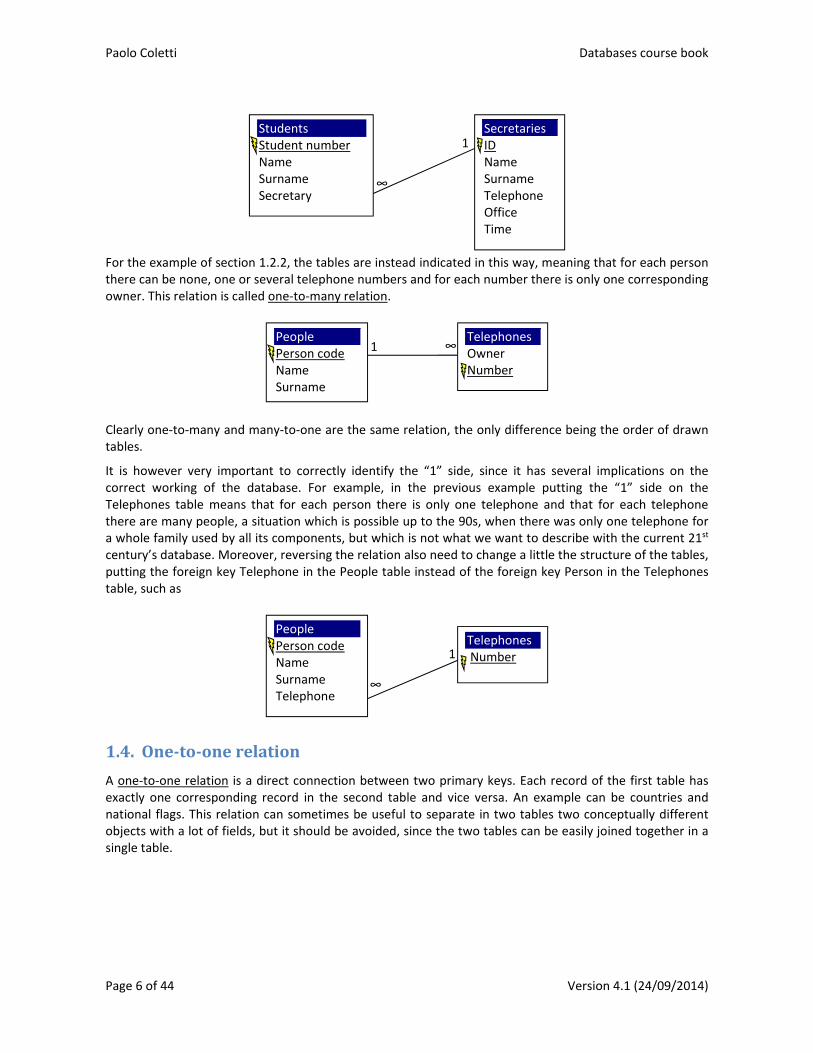
A relation is a connection between a field of table A (which becomes a foreign key) and the primary key of table B: on the B side the relation is “1”, meaning that for each record of table A there is one and only one corresponding record of table B, while on the A side the relation is “many” (indicated with the mathematical symbol ∞) meaning that for each record of table B there can be none, one or more corresponding records in table A.
For the example of section 1.2.1, the tables are indicated in this way, meaning that for each student there is exactly one secretary and for each secretary there are many students. This relation is called many‐to‐one relation.
Paolo Coletti Databases course book
Page 6 of 44 Version 4.1 (24/09/2014)
For the example of section 1.2.2, the tables are instead indicated in this way, meaning that for each person there can be none, one or several telephone numbers and for each number there is only one corresponding owner. This relation is called one‐to‐many relation.
Clearly one‐to‐many and many‐to‐one are the same relation, the only difference being the order of drawn tables.
It is however very important to correctly identify the “1” side, since it has several implications on the correct working of the database. For example, in the previous example putting the “1” side on the Telephones table means that for each person there is only one telephone and that for each telephone there are many people, a situation which is possible up to the 90s, when there was only one telephone for a whole family used by all its components, but which is not what we want to describe with the current 21st century’s database. Moreover, reversing the relation also need to change a little the structure of the tables, putting the foreign key Telephone in the People table instead of the foreign key Person in the Telephones table, such as
1.4. One‐to‐onerelation
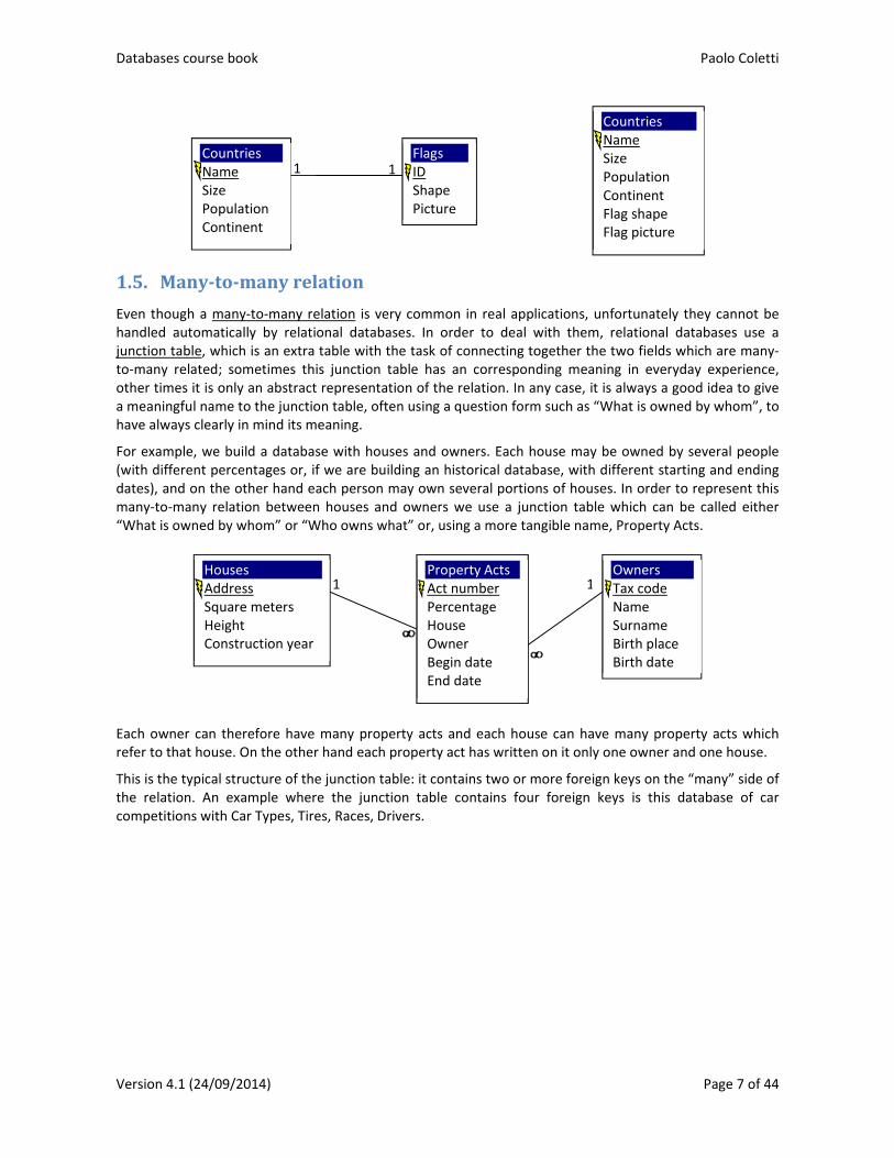
A one‐to‐one relation is a direct connection between two primary keys. Each record of the first table has exactly one corresponding record in the second table and vice versa. An example can be countries and national flags. This relation can sometimes be useful to separate in two tables two conceptually different objects with a lot of fields, but it should be avoided, since the two tables can be easily joined together in a single table.
∞
1Students Student number Name Surname Secretary
SecretariesID Name Surname Telephone Office Time
1 ∞People Person code Name Surname
TelephonesOwner Number
∞
1
People Person code Name Surname Telephone
Telephones Number
Databases course book Paolo Coletti
Version 4.1 (24/09/2014) Page 7 of 44
1.5. Many‐to‐manyrelation
Even though a many‐to‐many relation is very common in real applications, unfortunately they cannot be handled automatically by relational databases. In order to deal with them, relational databases use a junction table, which is an extra table with the task of connecting together the two fields which are many‐to‐many related; sometimes this junction table has an corresponding meaning in everyday experience, other times it is only an abstract representation of the relation. In any case, it is always a good idea to give a meaningful name to the junction table, often using a question form such as “What is owned by whom”, to have always clearly in mind its meaning.
For example, we build a database with houses and owners. Each house may be owned by several people (with different percentages or, if we are building an historical database, with different starting and ending dates), and on the other hand each person may own several portions of houses. In order to represent this many‐to‐many relation between houses and owners we use a junction table which can be called either “What is owned by whom” or “Who owns what” or, using a more tangible name, Property Acts.
Each owner can therefore have many property acts and each house can have many property acts which refer to that house. On the other hand each property act has written on it only one owner and one house.
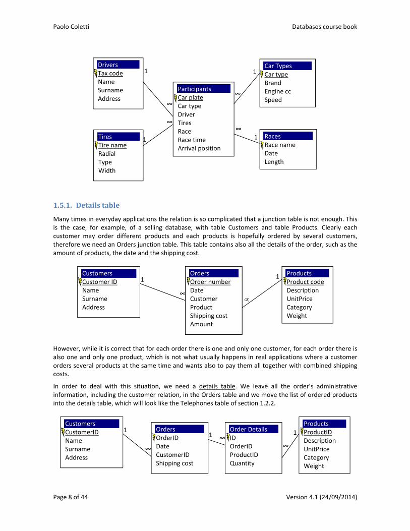
This is the typical structure of the junction table: it contains two or more foreign keys on the “many” side of the relation. An example where the junction table contains four foreign keys is this database of car competitions with Car Types, Tires, Races, Drivers.
1 1Countries Name Size Population Continent
FlagsID Shape Picture
Countries Name Size Population Continent Flag shape Flag picture
11 Houses Address Square meters Height Construction year
Owners Tax code Name Surname Birth place Birth date
Property ActsAct number Percentage House Owner Begin date End date
Paolo Coletti Databases course book
Page 8 of 44 Version 4.1 (24/09/2014)
1.5.1. Detailstable
Many times in everyday applications the relation is so complicated that a junction table is not enough. This is the case, for example, of a selling database, with table Customers and table Products. Clearly each customer may order different products and each products is hopefully ordered by several customers, therefore we need an Orders junction table. This table contains also all the details of the order, such as the amount of products, the date and the shipping cost.
However, while it is correct that for each order there is one and only one customer, for each order there is also one and only one product, which is not what usually happens in real applications where a customer orders several products at the same time and wants also to pay them all together with combined shipping costs.
In order to deal with this situation, we need a details table. We leave all the order’s administrative information, including the customer relation, in the Orders table and we move the list of ordered products into the details table, which will look like the Telephones table of section 1.2.2.
∞
1
∞
∞
1
1Car Types Car type Brand Engine cc Speed
∞
1 Drivers Tax code Name Surname Address
Tires Tire name Radial Type Width
RacesRace name Date Length
ParticipantsCar plate Car type Driver Tires Race Race time Arrival position
1 Products Product code Description UnitPrice Category Weight
∞
1 Customers Customer ID Name Surname Address
OrdersOrder number Date Customer Product Shipping cost Amount
∞∞
1 1
Products ProductID Description UnitPrice Category Weight
∞
1 Customers CustomerID Name Surname Address
OrdersOrderID Date CustomerID Shipping cost
Order DetailsID OrderID ProductID Quantity
Databases course book Paolo Coletti
Version 4.1 (24/09/2014) Page 9 of 44
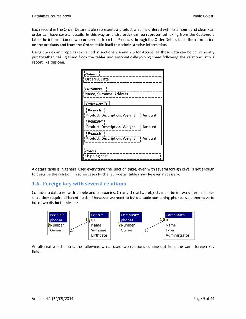
Each record in the Order Details table represents a product which is ordered with its amount and clearly an order can have several details. In this way an entire order can be represented taking from the Customers table the information on who ordered it, from the Products through the Order Details table the information on the products and from the Orders table itself the administrative information.
Using queries and reports (explained in sections 2.4 and 2.5 for Access) all these data can be conveniently put together, taking them from the tables and automatically joining them following the relations, into a report like this one.
A details table is in general used every time the junction table, even with several foreign keys, is not enough to describe the relation. In some cases further sub‐detail tables may be even necessary.
1.6. Foreignkeywithseveralrelations
Consider a database with people and companies. Clearly these two objects must be in two different tables since they require different fields. If however we need to build a table containing phones we either have to build two distinct tables as:
An alternative schema is the following, which uses two relations coming out from the same foreign key field:
Orders
OrderID, Date Customers
Name, Surname, Address Order Details
Products
Product, Description, Weight Amount
Products
Product, Description, Weight Amount
Products
Product, Description, Weight Amount
Orders
Shipping cost
People’s phones Number Owner ∞
1 PeopleID Name Surname Birthdate
∞
1Companies ID Name Type Administrator
Companies’phones Number Owner
Paolo Coletti Databases course book
Page 10 of 44 Version 4.1 (24/09/2014)
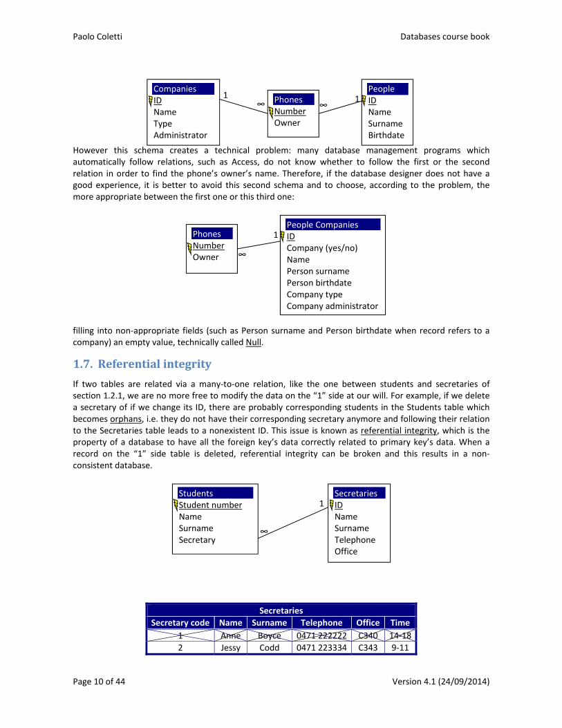
However this schema creates a technical problem: many database management programs which automatically follow relations, such as Access, do not know whether to follow the first or the second relation in order to find the phone’s owner’s name. Therefore, if the database designer does not have a good experience, it is better to avoid this second schema and to choose, according to the problem, the more appropriate between the first one or this third one:
filling into non‐appropriate fields (such as Person surname and Person birthdate when record refers to a company) an empty value, technically called Null.
1.7. Referentialintegrity
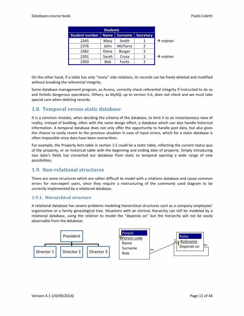
If two tables are related via a many‐to‐one relation, like the one between students and secretaries of section 1.2.1, we are no more free to modify the data on the “1” side at our will. For example, if we delete a secretary of if we change its ID, there are probably corresponding students in the Students table which becomes orphans, i.e. they do not have their corresponding secretary anymore and following their relation to the Secretaries table leads to a nonexistent ID. This issue is known as referential integrity, which is the property of a database to have all the foreign key’s data correctly related to primary key’s data. When a record on the “1” side table is deleted, referential integrity can be broken and this results in a non‐consistent database.
Secretaries
Secretary code Name Surname Telephone Office Time
1 Anne Boyce 0471 222222 C340 14‐18
2 Jessy Codd 0471 223334 C343 9‐11
Phones Number Owner
∞ ∞1
People ID Name Surname Birthdate
Companies ID Name Type Administrator
1
Phones Number Owner ∞
1People CompaniesID Company (yes/no) Name Person surname Person birthdate Company type Company administrator
∞
1Students Student number Name Surname Secretary
Secretaries ID Name Surname Telephone Office
Databases course book Paolo Coletti
Version 4.1 (24/09/2014) Page 11 of 44
Students
Student number Name Surname Secretary
2345 Mary Smith 1 orphan
2376 John McFlurry 2
2382 Elena Burger 2
2391 Sarah Crusa 1 orphan
2393 Bob Fochs 2
On the other hand, if a table has only “many” side relations, its records can be freely deleted and modified without breaking the referential integrity.
Some database management program, as Access, correctly check referential integrity if instructed to do so and forbids dangerous operations. Others, as MySQL up to version 5.6, does not check and we must take special care when deleting records.
1.8. Temporalversusstaticdatabase
It is a common mistake, when deciding the schema of the database, to limit it to an instantaneous view of reality, instead of building, often with the same design effort, a database which can also handle historical information. A temporal database does not only offer the opportunity to handle past data, but also gives the chance to easily revert to the previous situation in case of input errors, which for a static database is often impossible since data have been overwritten.
For example, the Property Acts table in section 1.5 could be a static table, reflecting the current status quo of the property, or an historical table with the beginning and ending date of property. Simply introducing two date’s fields has converted our database from static to temporal opening a wide range of new possibilities.
1.9. Non‐relationalstructures
There are some structures which are rather difficult to model with a relations database and cause common errors for non‐expert users, since they require a restructuring of the commonly used diagram to be correctly implemented by a relational database.
1.9.1. Hierarchicalstructure
A relational database has severe problems modeling hierarchical structures such as a company employees’ organization or a family genealogical tree. Situations with an intrinsic hierarchy can still be modeled by a relational database, using the relation to model the “depends on” but the hierarchy will not be easily observable from the database;
President
Director 1 Director 2 Director 3
∞∞
1
People Person code Name Surname Role
Roles Rolename Depends on
Paolo Coletti Databases course book
Page 12 of 44 Version 4.1 (24/09/2014)
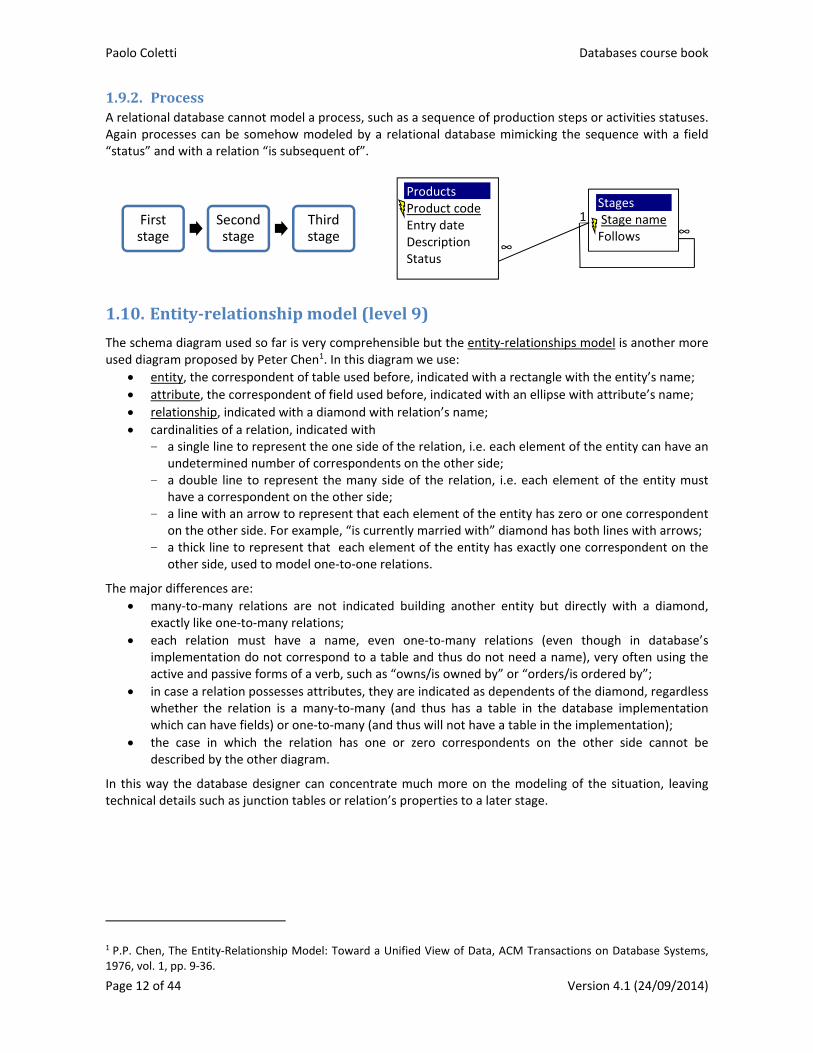
1.9.2. ProcessA relational database cannot model a process, such as a sequence of production steps or activities statuses. Again processes can be somehow modeled by a relational database mimicking the sequence with a field “status” and with a relation “is subsequent of”.
1.10. Entity‐relationshipmodel(level9)
The schema diagram used so far is very comprehensible but the entity‐relationships model is another more used diagram proposed by Peter Chen1. In this diagram we use:
entity, the correspondent of table used before, indicated with a rectangle with the entity’s name;
attribute, the correspondent of field used before, indicated with an ellipse with attribute’s name;
relationship, indicated with a diamond with relation’s name;
cardinalities of a relation, indicated with - a single line to represent the one side of the relation, i.e. each element of the entity can have an
undetermined number of correspondents on the other side; - a double line to represent the many side of the relation, i.e. each element of the entity must
have a correspondent on the other side; - a line with an arrow to represent that each element of the entity has zero or one correspondent
on the other side. For example, “is currently married with” diamond has both lines with arrows; - a thick line to represent that each element of the entity has exactly one correspondent on the
other side, used to model one‐to‐one relations.
The major differences are:
many‐to‐many relations are not indicated building another entity but directly with a diamond, exactly like one‐to‐many relations;
each relation must have a name, even one‐to‐many relations (even though in database’s implementation do not correspond to a table and thus do not need a name), very often using the active and passive forms of a verb, such as “owns/is owned by” or “orders/is ordered by”;
in case a relation possesses attributes, they are indicated as dependents of the diamond, regardless whether the relation is a many‐to‐many (and thus has a table in the database implementation which can have fields) or one‐to‐many (and thus will not have a table in the implementation);
the case in which the relation has one or zero correspondents on the other side cannot be described by the other diagram.
In this way the database designer can concentrate much more on the modeling of the situation, leaving technical details such as junction tables or relation’s properties to a later stage.
1 P.P. Chen, The Entity‐Relationship Model: Toward a Unified View of Data, ACM Transactions on Database Systems, 1976, vol. 1, pp. 9‐36.
First stage
Second stage
Third stage ∞
∞
1
ProductsProduct code Entry date Description Status
Stages Stage name Follows

Databases course book Paolo Coletti
Version 4.1 (24/09/2014) Page 13 of 44
1.10.1. Enhancedentity‐relationshipmodel
An enhanced entity‐relationships model is an improvement which permits also the existence of subclass, an entity which inherits all the attributes and relationships of another entity called superclass, adding some extra attributes and relationships of its own. For example, a database “zoo” can have entity “animals” with attributes “scientific name” and “common name”, which can have as subclass the entity “birds” with the same two attributes and the extra one “average wingspan”. This permits the modeling of some hierarchical structures (see section 1.9.1 on page 11) and solves the problem of foreign keys with several relations (see section 1.6 on page 9).
is
assigned
to Student
Secretaries
ID
Name
Surname
St number
Name
Surname

Paolo Coletti Databases course book
Page 14 of 44 Version 4.1 (24/09/2014)
2. MicrosoftAccess(level1)
Microsoft Access 2010 is a database management program, a program which is in charge of handling data and extracting them following correctly the relations and doing other sorting and filtering operations. Moreover, Access takes care of preserving the correct structure of the database enforcing referential integrity (see section 1.6).
Other famous database management programs are Oracle, MySQL, PostgreSQL.
2.1. Basicoperations
Access behaves in a slight different way with respect to Word or Excel and Office users can easily become confused.
The most important thing to keep in mind is that Access automatically saves every data operation as soon as it is done, without needing to give the save command. Exceptionally only the last data modification can be undone, but not the others. This behavior is typical of databases, where several people must access the data at the same time and therefore data must always be up‐to‐date. There is a File Save2 command in Access, but it is typically used to save the objects (tables, queries, reports, forms) inside the database file, while there is no need to use it to save the whole database file on the hard disk. If we want to save the database file with another name or in another format, the right tool to do it is the command File Save Database As3.
When the database is opened, the main window usually appears on the left4. Choose from the drop down menu Object Types and then select All Access Objects. Each object category presents the list of all that objects together with two buttons to manually create another object or to create it with the help of a wizard tool.
2.1.1. Northwindexample
Microsoft Access provides an official database example called Northwind. It is better to download from the course’s website the 2003 version, which is much simpler.5
When this database (or any other one containing Visual Basic macros) is opened, Access usually displays a Security Warning6, which can be ignored clicking on Enable. Then, this database example presents at its activation a splash window, i.e. a graphical interface which leads the user to the most common operations7. Building graphical interfaces is beyond the scope of this book and it can be ignored arriving directly at the database main window, which is composed of a left window displaying all the database’s objects and a right window displaying the currently open object.
2 For Access 2007 Office button Save. 3 In Access 2007 Office button Save As Save the database in another format Office button Manage Back Up Database, while in Microsoft Access 2003 there is only the option File Backup Database. 4 In Access 2003 it is a floating window with the object types’ menu on the left and All Access Objects does not need to be selected. 5 Also Access 2007 and 2010 have a Northwind 2007 database, but it must be downloaded or generated from a template file. Moreover, it has a much more complicated structure which can mislead the novice user. Office 2007 users should copy the Northwind.mdb file from an Office 2003 system in C:\Microsoft Office\Office11\Samples, or, if a computer with Office 2003 is not available, search for this file on the Internet with the help of a search engine. 6 With Access 2007 click on Options Enable this Content, while Access 2003 displays instead three pop‐up windows to which “No” then “Yes” then “Open” should be answered; they can be permanently disabled choosing Tools Macro Security Low. 7 Access 2003 displays two splash windows.

Databases course book Paolo Coletti
Version 4.1 (24/09/2014) Page 15 of 44
2.1.2. Relationshipsdiagram(level3)
Access provides a tool to automatically display the database’s schema through command Database Tools Relationships Relationships8. This opens a graphical interface displaying tables, fields and relations.
This tool has however small problems:
if some tables are missing, right‐click Show all;
if nonexistent tables are displayed, often with an _1 extension, select them and press Del;
when closing the relationships diagram Access asks to save it. This only saves the layout of the diagram, the modified relations are instead saved immediately.
In the relationships diagram relations can be created, deleted and modified:
to delete a relation, select it right‐click Delete. Warning: this operation cannot be undone;
to modify a relation, double‐click on it. A graphical interface appears, which displays the two tables and the related fields together with the relation type, which is automatically decided by Access according to the structure of the tables and to the fields involved. Moreover, there is also a checkbox to enforce referential integrity: it is very important that this box is checked because in this way Access will forbid the deletion of records in the “1” side table when this operation breaks the referential integrity of this relation;
to create a relation between two fields, simply drag a field above the other. If at least one of the two fields is a primary key, Access automatically recognizes the relation’s type and the only remaining thing to do is to apply referential integrity.
It is always better to do any structure’s modification before filling the tables with data. Once data are inside, Access may refuse to do certain operations on relations when the present data are inconsistent with the new relations, or may delete data inside foreign key fields when they do not complain with the new relation.
Relations can also be built with Lookup Wizard, as described below. Using this tool Access creates at the same time the relation and, in the foreign key field, a user‐friendly drop‐down menu which speeds up data insertion.
2.2. Tables(level1)
Tables are accessed choosing Tables object in the main database window.
The best way to create a new table is Create Tables Table Design9. This icon opens an empty table in Design View, where fields can be added with the indication of the primary key, the field name, the field type and the field detailed description. Right‐clicking on the left column gives the possibility to define or remove a primary key, while the field type can be chosen from a drop down menu in third column.
Each existing table in the main database window can be opened double‐clicking on it. The table is displayed in Datasheet View, which is an Excel‐like way to look at the table and which is also a convenient way to edit or insert data. In order to see the table in Design View, we choose Home View Design View10.
2.2.1. Fieldtypes
It is very important to choose the correct field type because it helps the database to minimize the space allocation and to avoid wrong insertions. In Access the most important field types are:
8 For Access 2007 Database Tools Show/Hide Relationships, for Access 2003 File Relationships. 9 For Access 2003 instead choose “Create table in Design View” from the main database window. 10 For Access 2003 View Design View.

Paolo Coletti Databases course book
Page 16 of 44 Version 4.1 (24/09/2014)
Text, which contains up to 255 alphanumeric characters. This type is proper for names, addresses and every short text;
Memo, which contains up to 65,536 alphanumeric characters. This type is proper for long texts, such as curricula, abstracts and small articles;
Number, which contains numbers which can be manipulated through mathematical operations. This type must be used only for numerical information. It is a very common mistake to use it for numeric codes, such as telephone numbers, version numbers and ZIP codes. Numeric codes must use the text type, since they may start with 0 (telephone 0471012343 or ZIP 00100) or have a 0 as last decimal digit (version 7.10) and, in any case, mathematical operations with them must be forbidden;
Date/Time, which contains dates and times. Exactly like Excel, Access memorizes date and time together, using integer numbers for days. Therefore dates can be subtracted to obtain the difference in days, or numbers can be added or subtracted to them to go ahead in the future or back in the past;
Currency, which contains numbers with automatically a currency symbol;
Autonumber, a type which is used only by Access to create IDs;
Yes/No, a type with only two values;
OLE object, which contains other files, such as images or documents. These files may be embedded, which means that the database file automatically contains a duplicate of this file (thus making the database file larger) or linked, which mean that the database file simply contains the link to the file (thus making it unusable when the external file is not available);
Hyperlink, which contains an hyperlink usually to a web page or to an email address;
Lookup Wizard is not a real field type but the possibility to take field’s values from a predetermined list or from other tables.
LookupWizard(level3)
From the Lookup Wizard, choosing “I will take the values from another table”, Access automatically builds a relation with another table taking the current field as foreign key of the “many” side and the primary key of the selected table as “1” side of the relation. At the same time, during the building of this relation, Access asks which fields the user wants to display in the drop down‐menu. Since these fields are simply what will be displayed, not the real field involved in the relation (which is instead the primary key), it is convenient to choose the most meaningful fields for data editing (for example, name, surname and birth date of a person). At the end of the wizard procedure the relation is created but remember to enforce the referential integrity in the last screen11.
From the Lookup Wizard, choosing instead “I will type in the values that I want”, Access lets the user type in a predetermined list of values which will be offered every time the field is filled. The list is not mandatory and a different value can be manually typed in the field.
Mandatorypredeterminedlist(level3)
If the list of predetermined values should be instead mandatory, you have the option to choose during the wizard’s procedure that the list is mandatory.12 However, building the list in this way does not offer a flexible way of adding new values to the list.
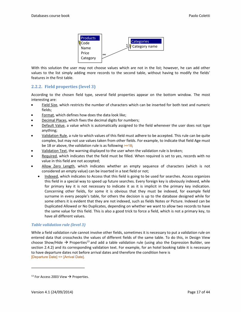
It is therefore much better to build them using another table which simply contains the list of values as primary key and build, via Lookup Wizard, a relation which takes values for this field from the primary key of the new table, such as in this example.
11 For Access 2003 and 2007: this option does not appear in the last screen and thus you should add manually the referential integrity from the relationships diagram (see section 3.3). 12 For Access 2003 and 2007: this option is not available, mandatory lists must be built only using another table.
Databases course book Paolo Coletti
Version 4.1 (24/09/2014) Page 17 of 44
With this solution the user may not choose values which are not in the list; however, he can add other values to the list simply adding more records to the second table, without having to modify the fields’ features in the first table.
2.2.2. Fieldproperties(level3)
According to the chosen field type, several field properties appear on the bottom window. The most interesting are:
Field Size, which restricts the number of characters which can be inserted for both text and numeric fields;
Format, which defines how does the data look like;
Decimal Places, which fixes the decimal digits for numbers;
Default Value, a value which is automatically assigned to the field whenever the user does not type anything;
Validation Rule, a rule to which values of this field must adhere to be accepted. This rule can be quite complex, but may not use values taken from other fields. For example, to indicate that field Age must be 18 or above, the validation rule is as following >=18;
Validation Text, the warning displayed to the user when the validation rule is broken;
Required, which indicates that the field must be filled. When required is set to yes, records with no value in this field are not accepted;
Allow Zero Length, which indicates whether an empty sequence of characters (which is not considered an empty value) can be inserted in a text field or not;
Indexed, which indicates to Access that this field is going to be used for searches. Access organizes this field in a special way to speed up future searches. Every foreign key is obviously indexed, while for primary key it is not necessary to indicate it as it is implicit in the primary key indication. Concerning other fields, for some it is obvious that they must be indexed, for example field surname in every people’s table, for others the decision is up to the database designed while for some others it is evident that they are not indexed, such as fields Notes or Picture. Indexed can be Duplicated Allowed or No Duplicates, depending on whether we want to allow two records to have the same value for this field. This is also a good trick to force a field, which is not a primary key, to have all different values.
Tablevalidationrule(level3)
While a field validation rule cannot involve other fields, sometimes it is necessary to put a validation rule on entered data that crosschecks the values of different fields of the same table. To do this, in Design View choose Show/Hide Properties13 and add a table validation rule (using also the Expression Builder, see section 2.4.2) and its corresponding validation text. For example, for an hotel booking table it is necessary to have departure dates not before arrival dates and therefore the condition here is [Departure Date] <= [Arrival Date].
13 For Access 2003 View Properties.
∞
1
Products Code Name Price Category
Categories Category name

Paolo Coletti Databases course book
Page 18 of 44 Version 4.1 (24/09/2014)
If more rules are needed, they must be combined with the And operator, for example ( [Departure Date] <= [Arrival Date] ) And ( [Booking Date] <= [Arrival Date] ).
Unfortunately the validation text is only one and it is not possible to tell the user exactly to which part of the rule his data do not adhere.
More complex expressions can be built with the Expression Builder (see section 2.4.2).
2.2.3. Importingtables(level3)
Access can obviously import data from several sources, typically tab‐delimited text files, comma‐separated text files and Excel files. The importing operation for text files is very similar to importing a text file into Excel. The importing operation of an Excel file is very easy with the command External Data Import & Link Excel14.
The only thing to pay attention to is that data must already be well structured before importing them into a table, otherwise the importing procedure will stop several times.
2.3. Forms(level3)
A form is a graphical interface which lets the user look, modify, insert, delete data. When the user is not the database administrator, it is better that tables are not accessed directly, since a wrong value, especially in a foreign key, can lead to a non‐consistent database. Forms can present the data in a more user‐friendly way and can restrict access to some data or forbid some data operations.
To produce a form in Access we build it using wizard choosing Create Forms Form Wizard15. This guides us through a step by step procedure, where we:
choose the tables and the fields from which data are taken. If data come from more than one table, Access automatically takes into consideration the existing relations and builds an appropriate subform for data on the “many” side. Data can also be taken from queries (see section 2.4), but usually they are not;
choose the layout of the form;
choose the style of the form;
assign to the form a name. The form, being an object, needs to be saved inside the database file.
The form can then be opened in Form View to access the data, paying attention to the fact that, as usual, every datum modification is automatically reflected in the corresponding table.
The form can also be opened in Design View to change its layout and style, or to add and remove fields. Choosing command Tools Properties16 opens all the form’s parts’ properties from which the layout can be precisely defined. Among these properties the most important ones are in the Form drop down menu Data tab, where modifying the fields “Allow Modifications”, “Allow Deletions” and “Allow Insertions” restricts the user from modifying, deleting, inserting records through this form.
If the Form Wizard does not work, as it can happen in case of a wrong installation of Access 2010, the form can be created without using the wizard clicking first on the main table that is to be used and then on Create Forms Form. This will create a form with all the fields of that table and the unnecessary ones can be later removed in Design View. In case a subform is needed, the table containing the data to be inserted in the subform can be simply dragged inside the existing form.
14 For Access 2007 External Data Import Excel, for Access 2003 File External data Import. 15 For Access 2007 Create Forms Other Forms Create using Wizard, for Access 2003 we instead choose “Create Form using wizard” from the database main window. 16 For Access 2003 View Properties.

Databases course book Paolo Coletti
Version 4.1 (24/09/2014) Page 19 of 44
2.4. Queries(level1)
A query is a question posed to the database, which answers with a virtual table called view. The question can be, for example, “Which students are born in 2007?” or “Who are the German students, which is their address, and what are their grades’ averages?”. The view would be in these cases a table with a single column with the students’ numbers, or a table with four columns with student’s name, student’s surname, student’s address and the average of the grades of that student.
The view therefore contains all the values corresponding to the fields selected in the query, organized following correctly the underlying relations, sorted and filtered according to the query’s indication and together with virtual fields created using formulas contained in the query. It is thus a powerful tool to extract information from the database.
The view, even though it is virtual, is directly linked to the real data and any modification to its data is automatically reflected in the original tables. The view does not contain any formatting: to present query’s results in a better‐looking format, report is the appropriate tool (see section 2.5).
2.4.1. Selectionqueries
The select query is the standard type of query, a direct question to the database which involves only data extraction following correctly the relations and sometimes doing calculations. For example, a question such “Which exams has Jack passed?” or “How many students has each secretary in charge?”.
To produce a select query in Access we simply use the command Create Queries Query Wizard17. This guides us through a step by step procedure, where we:
choose the tables and the fields from which data are taken. If data come from more than one table, Access automatically takes into consideration the existing relations. Data can also be taken from other queries;
give the query a name. The query, being an object, needs to be saved inside the database file.
The query can then be opened in Datasheet View to access the data, paying attention to the fact that, as usual, every datum modification is automatically reflected in the corresponding tables.
The query can also be opened in Design View, where we have full control over what is displayed in the view. In the upper side of this window we see the involved tables with their relations and we can add other tables with right‐click Add tables. In the lower side we have the selected fields, which can be removed with right‐click Del or to which other fields can be added simply dragging them from the tables above. To a field we can also put a sorting option, ascending or descending, or a Show option to display/hide the field (obviously hiding makes sense only when the field is used for something else, otherwise it would be better to remove it directly from the query).
If the Query Wizard does not work, as it can happen in case of a wrong installation of Access 2010, the query can be created directly in Design View clicking on Create Queries Query Design.
We can also use a criterion to filter out some records. For example, we can type in the criteria space directly a value (enclosed in quotations if that field is a textual field) and only the data having this value in this field are displayed. We can also put more complicated conditions, such as equalities and inequalities or conditions involving other fields. For example, to filter out underage students, we can put in the Age field criterion >=18, while to consider only students enrolled from 2013, we can put in the EnrollDate field criterion >= #1/1/2013#.
17 For Access 2007 Create Other Query Wizard, for Access 2003, we select the Queries objects in the main database window and choose “Build Query using Wizard”.
Paolo Coletti Databases course book
Page 20 of 44 Version 4.1 (24/09/2014)
However, when the condition becomes too complicated, it is better to use the Expression Builder (see section 2.4.2). If two criteria are put on the same field, typing them on two spaces one above the other, they automatically are alternative (it is enough that one of them be valid for those data to be displayed); on the other hand if two criteria are put on different fields, typing them on two spaces of the same row, they are considered together (both must be valid for those data to be displayed). Again, complicated conditions with logical operators are more easily built with the Expression Builder.
Virtualfields
Other fields can be automatically generated taking values from any field, even fields not present in the query (but their tables must be present in the query’s window upper part), and applying mathematical, logical or textual operations. We simply type in the field’s name space of an existing query the virtual field’s name followed by a colon and by its expression, using the Expression Builder (see section 2.4.2) or typing fields’ names involved in the operation enclosed in square brackets. For example, to build virtual field ToPay which contains the price of an order with a single product, we simply type in the field’s name space ToPay: [Price] * [Quantity].
If we instead type in the name’s space or in the criteria’s space something between square parenthesis which does not correspond to any field in the present tables, Access stops the execution of the query and asks us the value of that thing. This is a good trick to force Access to ask the user a value. For example, putting in the criteria space of the EnrolmentYear field [Please, tell me the enrolment year] and switching to Datasheet View, forces Access to stop the execution of the query, realize that a field with name “Please, tell me the enrolment year” does not exist, and display a dialog box which says exactly “Please, tell me the enrolment year”.
2.4.2. ExpressionBuilder(level1)
The Expression Builder is a powerful tool to build expressions, which can be called clicking on the three dots anytime there is the need for an expression, e.g. validation rules, table validation rules, query’s criteria and
query’s new fields. If the three dots are not present, click on the magic wand button .
The Expression Builder has a main space where the expression appears. It can be directly typed in or it can be built using the mathematical and logical operators presented below. If it is possible (i.e. we are not inside a field’s validation rule), other fields’ values can be inserted in the expression choosing them from the menus below: they appear as their field’s name enclosed in square parenthesis, sometimes preceded by the table’s name if the same field’s name is used in more than one table. Also many functions can be inserted, the most interesting being:
Date to get the current date;
DateDiff to get the difference in months or years between two dates;
DateAdd to get a date plus or minus a certain amount of months or years;
Year to get the year from a date, Month to get the month and Day to get the day;
the usual mathematical functions Abs, Exp, Sqr, Log, Int;
Like, which lets the user check whether the value corresponds to an expression using wildcards ? (any character) and * (any amount of characters). For example, to check that a ZIP code has exactly 5 characters and starts with 39, we can use the condition Like “39???”. To check that an email address is reasonable, we can use the condition Like “*@*.*”.
2.4.3. Summaryquery(level3)
A simple query is able to perform operations, but only acting within the same record of the view and is not able to perform operations involving different records, such as sums or averages. For example, “How many students has each secretary in charge in 2009?” or “What is the average students’ grade this year for each country?”.

Databases course book Paolo Coletti
Version 4.1 (24/09/2014) Page 21 of 44
To do this, we need a summary query: we create a simple query with the involved fields, then we press
Show/Hide Totals button18 and a new option appears in the query’s field. This option is originally set to Group By, meaning that the view will now be squeezed trying to group identical values of those fields. If some view’s records have the same values in all the fields which have the Group By option, only a single record appears in the view. This feature used alone can be applied to some rare situations (and, on the other hand, causes some problems when the summary query is wrongly chosen instead of a simple query), but usually it works in conjunction with the selection of another option for one field, such as Sum, Count or Avg. In this case, the query tries to group using the fields with the Group By and, for every group, it calculates the sum, average or count of the values of the field with the other option.
For example, if we have a database with Students table with Country field and we have an Exams table with Grade field and we want to calculate the average grade for each country, we need to create a query with these two fields, convert it to summary query, and then select Avg option to the Grade field while leaving Group By option to the Country field. The result is a view with field Country with the list of countries, each one appearing only once since the results are grouped by countries, and field Grade (sometimes called instead Avg of Grade) with the average of the values of the Grade fields for students in that country.
It is very important to remember that every field present in the query with the Group By option is used to group, even when this field has the no‐show option or when this field is simply used for a criterion. A wrong grouping, with extra fields, clearly produces more records in the view than what should be. Criteria in fields with Group By option can thus lead to problems and therefore it is always suggested to switch the Group By option to Where whenever a field is used only for filtering and not for grouping.
For example, if in the database above we want to calculate the average grade per country in 2008, we need to build a simple query with the fields Country, Grade and Date. Then we convert it to summary query, we select Avg option in the Grade field and we select Where in the Date field putting as criterion Between
#1/1/2008# and #31/12/2008# and we unselect the Show option. If we instead leave Group By option in the Date field with no‐show option and with this criterion, the result is grouped by country and by date which means that the view shows the average per country per exam session.
2.4.4. Nonselectionqueries(level9)
While selection queries extract data from the database, there are other queries which actively modify data in the database. The best way to handle these queries is to build them as selection queries in Design View and Datasheet View, then from the Query Type tab19 switch them to the appropriate query type, check carefully in Design View that the query is doing exactly what is wanted and then finally press Results Run20 to do changes to the data.
Make Table query converts the view into a real independent table. From now on those data are independent from the data contained in the original tables.
Update query selects records and can assign a value to the present fields through a new space that appears.
Delete query selects records and deletes all the records involved (and not only the content of the present fields) from their corresponding tables.
Append query appends the records of the view to an existing table. Obviously the view’s fields must match exactly the fields of the table.
18 In Access 2003 it is simply the ∑ button. 19 In Access 2003 from the Query menu. 20 For Access 2003 Query Run.

Paolo Coletti Databases course book
Page 22 of 44 Version 4.1 (24/09/2014)
2.5. Reports(level3)
A report is a way to present database’s data in a good‐looking format.
To produce a report in Access we simply use the command Create Reports Report Wizard21. This guides us through a step by step procedure, where we:
choose the tables or the queries and their fields from which data are taken;
choose whether data must be grouped or not. For example, students can be grouped by countries it the Country field is selected. If data from several tables are involved, Access always suggests a grouping based on the relation’s “1” side. Once the first grouping is selected, Access asks whether further grouping is required. For example, students can be grouped by corresponding secretary and then, inside each group, grouped again by country;
choose whether data must be sorted;
choose the layout of the report;
choose the style of the report;
give the report a name. The report, being an object, needs to be saved inside the database file.
The report is automatically opened in Print Preview22. Unfortunately closing Print Preview also closes the report23. Thus to be opened in another view, the report should be right‐clicked to choose Report View to look at the final result or Design View to change its layout and style, to add and remove fields, titles, header and footer. Grouping and sorting may be modified clicking on Design Grouping & Totals Groups & Sort.
Reports can be exported from Access in RTF format from Data More Word24.
If the Report Wizard does not work, as it can happen in case of a wrong installation of Access 2010, the form can be created without using the wizard clicking first on the main table that is to be used and then on Create Reports Report. This will create a form with all the fields of that table and the unnecessary ones can be later removed in Design View, together with grouping’s and sorting’s modifications.
21 In Access 2003, we select the Reports objects in the main database window and choose “Build Report using Wizard”. 22 In Access 2003 it is opened automatically in Report View. 23 This happens only in Access 2010. For Access 2003 and 2007, closing the Print Preview jumps to another view. 24 For Access 2003 and 2007 Data Word
Databases course book Paolo Coletti
Version 4.1 (24/09/2014) Page 23 of 44
3. MySQL(level5)
MySQL is a free SQL database management program, a program which is in charge of storing data and letting users extract, modify, insert them using SQL language (see section 0).
Unlike Microsoft Access, MySQL program runs as a server on a computer and receives SQL connections on port 3306. These connections may come from the same computer or from external ones called clients, in case port 3306 is open for external connections. To each client request, MySQL server returns an answer always in textual form which may be a table, in case of data request, a simple acknowledge in case of a command request or an error message.
Unlike Microsoft Access 2010, MySQL uses user authentication, i.e. the user must provide a valid username and password to open a connection from his client to MySQL server and must have the privileges for the operation he is trying to do. For example, an user without the ALTER TABLE privilege will be unable to change the structure of a table.
3.1. HeidiSQL
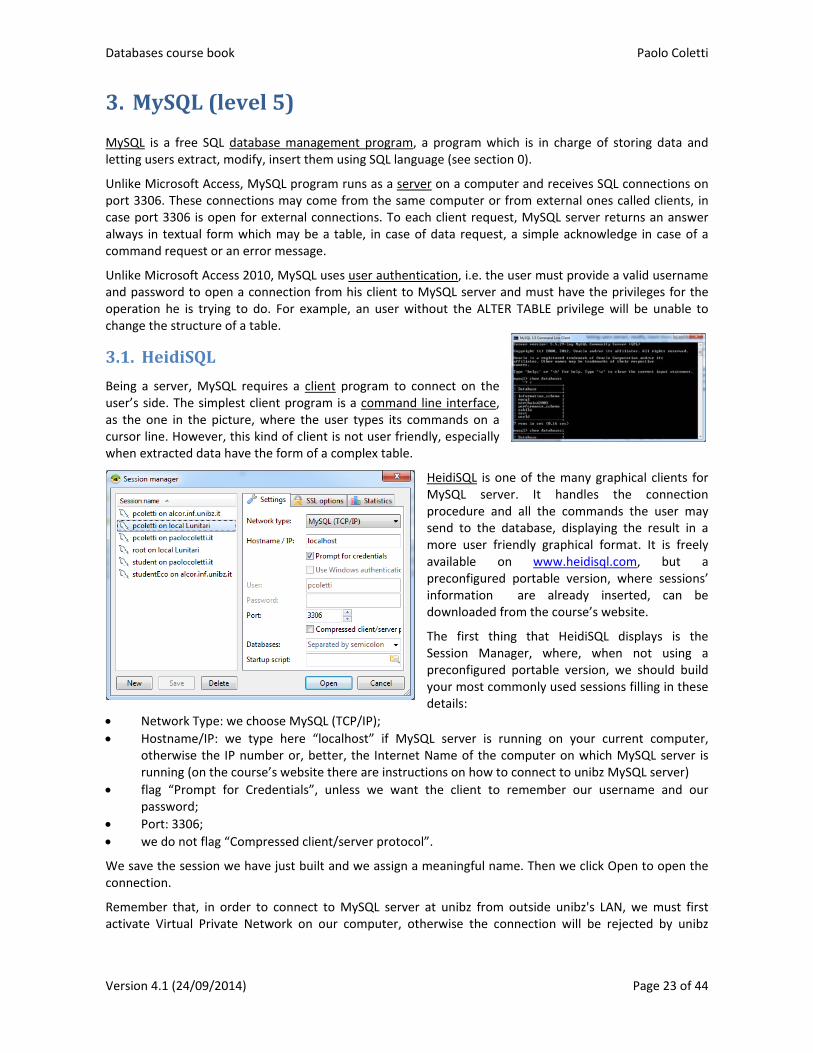
Being a server, MySQL requires a client program to connect on the user’s side. The simplest client program is a command line interface, as the one in the picture, where the user types its commands on a cursor line. However, this kind of client is not user friendly, especially when extracted data have the form of a complex table.
HeidiSQL is one of the many graphical clients for MySQL server. It handles the connection procedure and all the commands the user may send to the database, displaying the result in a more user friendly graphical format. It is freely available on www.heidisql.com, but a preconfigured portable version, where sessions’ information are already inserted, can be downloaded from the course’s website.
The first thing that HeidiSQL displays is the Session Manager, where, when not using a preconfigured portable version, we should build your most commonly used sessions filling in these details:
Network Type: we choose MySQL (TCP/IP);
Hostname/IP: we type here “localhost” if MySQL server is running on your current computer, otherwise the IP number or, better, the Internet Name of the computer on which MySQL server is running (on the course’s website there are instructions on how to connect to unibz MySQL server)
flag “Prompt for Credentials”, unless we want the client to remember our username and our password;
Port: 3306;
we do not flag “Compressed client/server protocol”.
We save the session we have just built and we assign a meaningful name. Then we click Open to open the connection.
Remember that, in order to connect to MySQL server at unibz from outside unibz's LAN, we must first activate Virtual Private Network on our computer, otherwise the connection will be rejected by unibz
Paolo Coletti Databases course book
Page 24 of 44 Version 4.1 (24/09/2014)
firewall as untrustworthy. Instructions on how to set up VPN are on http://www.unibz.it/en/ict/ComputerInternet/network/vpn .
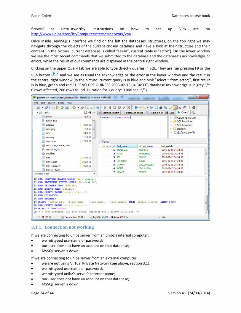
Once inside HeidiSQL’s interface we find on the left the databases’ structures, on the top right we may navigate through the objects of the current chosen database and have a look at their structure and their content (in the picture: current database is called “sakila”, current table is “actor”). On the lower window we see the most recent commands that we submitted to the database and the database’s acknowledges or errors, while the result of our commands are displayed in the central right window.
Clicking on the upper Query tab we are able to type directly queries in SQL. They are run pressing F9 or the
Run button and we see as usual the acknowledge or the error in the lower window and the result in the central right window (in the picture: current query is in blue and pink “select * from actor;”, first result is in blue, green and red “1 PENELOPE GUINESS 2006‐02‐15 04:34:33”, database acknowledge is in grey “/* 0 rows affected, 200 rows found. Duration for 1 query: 0,000 sec. */”).
3.1.1. Connectionnotworking
If we are connecting to unibz server from an unibz’s internal computer:
we mistyped username or password;
our user does not have an account on that database;
MySQL server is down.
If we are connecting to unibz server from an external computer:
we are not using Virtual Private Network (see above, section 3.1);
we mistyped username or password;
we mistyped unibz’s server’s Internet name;
our user does not have an account on that database;
MySQL server is down;
Databases course book Paolo Coletti
Version 4.1 (24/09/2014) Page 25 of 44
we are not connected to the Internet;
our firewall prevents outgoing connections from port 3306;
If we are connecting to another server on your same computer: in this case we should try to use the command line interface to check whether server is up and our password works, as described at the end of procedure in section 3.2).
If we are connecting to another external server:
we mistyped username or password;
we mistyped the server’s Internet name;
our user does not have an account on that database;
MySQL server is down;
our user does not have the privilege to connect to MySQL server from outside (a check on which computer we are is performed every time we connect by MySQL server);
we are not connected to the Internet;
our firewall prevents outgoing connections from port 3306;
the firewall on which MySQL is running prevents incoming connections on port 3306.
3.2. InstallingMySQLserver
While it is not necessary to install a MySQL server as there are others available to do exercises, it may be a convenient choice to install a local MySQL server which will allow our client to make faster connections and work also without Internet connection.
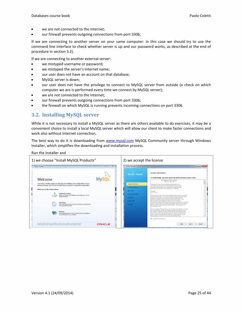
The best way to do it is downloading from www.mysql.com MySQL Community server through Windows Installer, which simplifies the downloading and installation process.
Run the installer and
1) we choose “Install MySQL Products” 2) we accept the license
Paolo Coletti Databases course book
Page 26 of 44 Version 4.1 (24/09/2014)
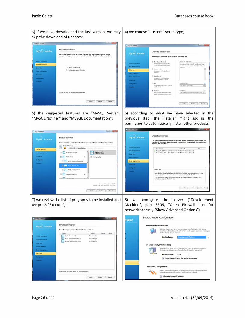
3) if we have downloaded the last version, we may skip the download of updates;
4) we choose “Custom” setup type;
5) the suggested features are “MySQL Server”, “MySQL Notifier” and “MySQL Documentation”;
6) according to what we have selected in the previous step, the installer might ask us the permission to automatically install other products;
7) we review the list of programs to be installed and we press “Execute”;
8) we configure the server (“Development Machine”, port 3306, “Open Firewall port for network access”, “Show Advanced Options”)
Databases course book Paolo Coletti
Version 4.1 (24/09/2014) Page 27 of 44
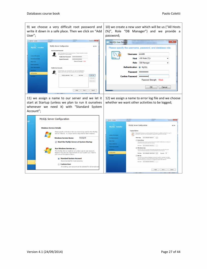
9) we choose a very difficult root password and write it down in a safe place. Then we click on “Add User”;
10) we create a new user which will be us (“All Hosts (%)”, Role “DB Manager”) and we provide a password;
11) we assign a name to our server and we let it start at Startup (unless we plan to run it ourselves whenever we need it) with “Standard System Account”;
12) we assign a name to error log file and we choose whether we want other activities to be logged;
Paolo Coletti Databases course book
Page 28 of 44 Version 4.1 (24/09/2014)
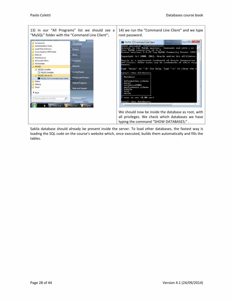
13) in our “All Programs” list we should see a “MySQL” folder with the “Command Line Client”;
14) we run the “Command Line Client” and we type root password.
We should now be inside the database as root, with all privileges. We check which databases we have typing the command “SHOW DATABASES;” .
Sakila database should already be present inside the server. To load other databases, the fastest way is loading the SQL code on the course’s website which, once executed, builds them automatically and fills the tables.
Databases course book Paolo Coletti
Version 4.1 (24/09/2014) Page 29 of 44
4. SQLlanguageforMySQL(level5)
SQL is a structured query language for extracting and modifying data and managing databases. Its commands are typed directly into MySQL client and executed. In particular, using HeidiSQL we type them in
the Query window and we run them pressing F9 or the Run button . The Query window can be
saved as a SQL file pressing CTRL+S or the Save SQL to File button . A new Query window can be created
pressing on the appropriate tab . The entered commands are repeated in the lowest window, together with the MySQL’s acknowledge or error message. Also this window can be saved right‐clicking the mouse on it and choosing Save as textfile.
SQL commands can be entered with keywords written in capital or small caps, it does not matter. Traditionally capital letters are used for keywords to make the code more readable. They must always end with a semicolon.
In HeidiSQL pressing F1 while a keyword is highlighted calls the SQL help, where we get a detailed description of the syntax.
4.1. Basicoperations
The first SQL command to operate with a database is USE {database}; for example to use the database Sakila USE sakila;. In HeidiSQL we simply click on a database on the left window and a USE {database}; command is immediately executed.
Once the database is chosen, activities on this database’s tables can be done. However, in order to perform them, the user must have proper authorization. A different authorization can be assigned to the user on each different table of each database, but usually the administrator assigns the same authorization on all the tables of the same database. Authorizations include GRANT SELECT to perform select queries, GRANT
INSERT to insert data, GRANT UPDATE to modify data, GRANT DELETE to delete data, GRANT ALTER to modify the table’s structure.
Special care must be taken before performing operations which modify the data or the structure. While some versions of MySQL database offer the possibility to undo the last performed operation using ROLLBACK; command, many others do not. Thus, while simply looking at data or performing selection queries does not cause any harm, we must think twice before modifying data or changing the structure of a table.
4.2. Simpleselectionqueries
A query is a question posed to the database, which answers with a temporary table of data. In HeidiSQL this temporary table is displayed immediately below the window where the command is entered.
The question can be, for example, “Which students are born in 2007?” or “Who are the German students, which is their address, and what are their grades’ averages?”. The result would be in these cases a temporary table with a single column with the students’ numbers, or a temporary table with four columns with student’s name, student’s surname, student’s address and the average of the grades of that student.
The result therefore contains all the values corresponding to the fields selected in the query, organized following the underlying relations according to the query’s indication, sorted and filtered according to the query’s indication and together with virtual fields created using formulas contained in the query. It is thus a powerful tool to extract information from the database.
The selection query is the basic type of query, a direct question to the database which involves only data extraction following correctly the relations and sometimes doing calculations. For example, a question such “Which exams has Jack passed?” or “How many students has each secretary in charge?”.

Paolo Coletti Databases course book
Page 30 of 44 Version 4.1 (24/09/2014)
The basic SQL syntax for a selection query is SELECT {fields} FROM {table}; where {fields} is a list of fields separated by commas and {table} is the name of a table. For example, SELECT FirstName, LastName, BirthDate FROM Students; produces a temporary table with 3 columns extracted from permanent table Students, which probably contains many more fields.
To add a filtering or sorting condition we just need to add, after the table’s name and before the semicolon, WHERE {condition} ORDER BY {field} {ASC|DESC} For example, SELECT FirstName, LastName FROM Students WHERE ( Enrolment_Date >= ‘2013-01-01’ ) ORDER BY LastName ASC ORDER BY FirstName ASC; produces a list of students enrolled from 2013, ordered first by surname and, in case two students have the same surname, by first name.
Query SELECT FirstName, LastName, Residence_address, Residence_Country FROM Students WHERE ( ( Enrolment_Date >= ‘2013-01-01’ ) AND ( Residence_country = ‘Germany’ ) ); produces a list of students with their addresses enrolled from 2013 and resident in Germany, in no particular order. Note that the condition may involve a field which is or which is not in the query fields, but the field must obviously be in the selected table. Spaces in the condition and parenthesis around the condition are not mandatory, but improve readability and are very helpful when conditions become complicated.
There are other operators and functions which are helpful in conditions:
the usual mathematical operators +, -, *, /
the usual mathematical comparisons =, <, >, <=, =>, <>
{field} BETWEEN {value1} AND {value2}, for example Price BETWEEN 20 and 50
{condition1} AND {condition2}, for example ( Price > 50 ) AND ( Quantity < 20 )
{condition1} OR {condition2}, for example ( Price > 50 ) OR ( Quantity < 20 )
NOT {condition}, which reverses the condition after it, for example NOT (Country = ‘Germany’)
IS NULL and IS NOT NULL, to check whether a value is empty or not, such as (‘End date’ IS NOT NULL)
{field} IN ({list}), very useful when you need to filter in values in a list, for example Country IN (‘Germany’,‘Italy’,‘Austria’,‘France’)
{field} LIKE {expression}, for approximated matching filters, such as Surname LIKE ‘Col%’, which selects only surnames starting with Col, or Surname LIKE ‘Col_t’ which selects only surnames such as Colet, Colit, Coltt, Col t, Col4t, etc.
CURDATE(), to be used in expression where current date (with midnight time) is needed, for example to select students enrolled today Enrolment_Date = CURDATE(). Pay special attention when you compare this function with a date including time, as this function gives you the current date with midnight time and can give you the wrong result; for example Enrolment_Time <=
CURDATE() does not return people enrolled today
DATE_ADD({date},{interval}) to add (or subtract when the interval is negative) days, months, years from a date, for example DATE_ADD('2012-01-09', INTERVAL 14 MONTH) results in ‘2013-03-09’
YEAR({date}) to get the year from a date, such as YEAR(Enrolment_Date) = 2012
MONTH({date}) to get the numerical month from a date, such as MONTH(Enrolment_Date) = 9
DAY({date}) to get the day of the month from a date, such as DAY( CURDATE() ) = 1, which is true only when today is the first day of the month,
unfortunately SQL does not have, as Access, a function to directly calculate the difference in years between two dates, since function DATEDIFF() returns the difference in days and not in years. Therefore, the two ways to get the difference in years between two dates is the approximate way ROUND(DATEDIFF({date2},{date1})/365.25) and this trick for the exact difference YEAR({date2}) -
YEAR({date1}) - ( DATE_FORMAT( {date2}, '%m%d' ) < DATE_FORMAT( {date1}, '%m%d' ) ).

Databases course book Paolo Coletti
Version 4.1 (24/09/2014) Page 31 of 44
4.2.1. Virtualfields
New virtual fields for the resulting temporary table can be automatically generated taking values from any field, even fields not present in the query (but they must be present in the tables used by the query), and applying mathematical, logical or textual operations. We simply write AS after the expression: SELECT {expression} AS {name} FROM {table}; For example, to build virtual field ToPay which contains the price of an order with a single product, we simply type in the field’s list SELECT ProductName, Price * 0.9 AS Discounted_Price FROM Products; To build a virtual field as a sum of two other fields SELECT StudentID, Tax_First_Semester+Tax_Second_Semester AS TotalTax FROM Taxes;
4.2.2. Views
In case we plan to use the query again in the future or we simply want to save it inside the database or we plan to use its temporary table as a source table for another query, it is a good idea to make it permanent creating a view with CREATE VIEW {name} AS {query}; For example, CREATE VIEW List_Of_Discounted_Products AS SELECT ProductName, ProductDescription, Price * 0.9 AS Discounted_Price FROM Products; This query can be used later by another query as a source table, for example SELECT ProductName, Discounted_Price FROM List_Of_Discounted_Products ORDER BY ProductName ASC;
To destroy a view, usually because we want to rebuild it in another way: DROP VIEW {name};
4.3. Innerjoins
If we want to take values from two tables, SQL language is not able to correctly follow the relations unless it is explicitly instructed to do so. This is due to the fact that SQL is a generic programming language which works for every database management program, even those which do not handle automatic relations nor referential integrity. Therefore, we need to remind SQL which relations are involved and how they work. The syntax is SELECT {fields} FROM {table1} INNER JOIN {table2} ON {field1} = {field2}; where {field1} and {field2} are the foreign and primary key of related tables, while {fields} are the names of the selected fields from {table1} and {table2}. For example, SELECT Name, Surname, Number FROM People INNER JOIN Telephones ON Person_code=Owner; or SELECT Name, Surname, `Arrival position` FROM Drivers INNER JOIN Participants ON `Tax code`=Driver;
In case the same field’s name is used in both tables, field’s names must be preceded by table’s name and a dot. For example, SELECT Secretaries.FirstName, Secretaries.LastName, Students.LastName FROM Students INNER JOIN Secretaries ON Secretaries.Code = Students.Secretary; In this way it is much clearer where each field comes from.
Obviously to these queries filtering conditions with WHERE, sorting conditions with ORDER BY and renaming of fields with AS can be used.
Moreover, since sometimes the table name might be rather long and boring to rewrite it several times, the AS operator may be used also to rename a table, such as SELECT b.FirstName, b.LastName, a.LastName FROM Students AS a, INNER JOIN Secretaries AS b ON a.Code = b.Secretary;

Paolo Coletti Databases course book
Page 32 of 44 Version 4.1 (24/09/2014)
4.3.1. Crossjoins
A cross join is a query involving several tables without performing any join, such as using tables in section 1.2.2 SELECT People.Name, People.Surname, Telephones.Number FROM People, Telephones; The result is the global combination of all the fields of all the tables. In the example’s case, a huge table with “John Smith” and all the 19 telephone numbers, then “John McFlurry” and all the same 19 telephone numbers, etc. This is very rarely what is wanted from the database, even though sometimes it might be.
4.3.2. Multipleinnerjoins
When three or more tables are involved, there must be a compound inner join, even when a table (typically a junction table) does not use any field. Using the example in section 1.5, SELECT Houses.SquareMeters, Owners.LastName FROM ( Houses INNER JOIN PropertyActs ON Address = PropertyActs.House ) INNER JOIN Owners ON PropertyActs.Owner = TaxCode; Even though the inner join seems more difficult to use, it exactly describes what the query is doing: taking all three tables and squeezing their content relation by relation until a single table is reached.
Another example using the details table in section 1.5.1, written in several lines just to improve readability, SELECT c.Surname, c.Name, p.ProductName, od.Quantity, p.UnitPrice FROM ( ( ( Orders INNER JOIN ‘order details’ AS od ON Orders.OrderID = od.OrderID ) INNER JOIN Products AS p ON od.ProductID = p.ProductID ) INNER JOIN Customers AS c ON c.CustomerID = Orders.CustomerID ); As is it evident, using the same field name for the primary and the foreign key makes detecting the relations much easier. A
Another good trick is avoiding any strange character and any space in tables’ and fields’ names, otherwise they must be enclosed in the special quotation symbol grave accent `.25 We must take special care that the symbol is not the usual apostrophe or single quotation ‘, which instead is used for values such as text and dates, but the one in the opposite direction as the grave accent. For example, to displays all the houses and their current owners (for whom End date is either Null or it is in the future) SELECT Address, `Square meters`, p.Percentage, Owners.Name, Owners.Surname FROM ( ( Houses INNER JOIN `Property Acts` AS p ON Houses.Address=p.House) INNER JOIN Owners ON Owner=`Tax code` ) WHERE ( ( p.`Begin date` <= CURDATE() ) AND ( ( p.`End date` IS NULL ) OR ( p.`End date`>CURDATE() ) );
DifferencebetweenWHEREandON
Theoretically an inner join query could be rewritten as a cross join table using WHERE condition and produce the same result. For example SELECT Name, Surname, Number FROM People INNER JOIN Telephones ON Person_code=Owner; and SELECT Name, Surname, Number FROM People, Telephones WHERE Person_code=Owner; produces exactly the same result. The second query, however, performs first a cross join which produces a very large table and then reduces it with a filter. While for small amounts of data this is not a problem, when the number of involved tables and records increases, a query performed in this way is inefficient and can be very slow. Moreover, the latter query is misleading from a theoretical point of view and can confuse user who must check and modify it further.
25 In case this symbol does not appear on the keyboard, in HeidiSQL any table or field name can be easily produced, together with the enclosing symbol, double clicking on the table’s or field’s name. Producing it directly withgout copying and pasting it from another part of the code is rather complicated: we press Windows key + R, then we type “charmap”, then we go through the character map until we find the grave accent, we copy and paste it.

Databases course book Paolo Coletti
Version 4.1 (24/09/2014) Page 33 of 44
4.4. Summaryqueries
A simple selection query is able to perform calculation’s operations to create virtual fields, but only acting record by record, while it is not able to perform operations involving different records, such as sums or averages. For example, “How many students has each secretary in charge in 2009?” or “What is the average students’ grade this year for each country?”.
To do this, we need a summary query. Their syntax is exaclty the same of the simple query, with the two differences that an aggregation function (Sum, Avg, Max, Min, Count(*), Count(DISTINCT {field})) is applied to the field on which a record by record operation must be done and that a GROUP BY {fields} is optionally appended at the end of the SQL command. Scope of the GROUP BY is to aggregate the records all together, ending up with one record per value of the grouping fields.
For example, if we have a database with Students table with Country field and we have an Exams table with Grade field and we want to calculate the average and minimum grade for each country, the SQL is SELECT Country, Avg(Grade), Min(Grade) FROM Students INNER JOIN Exams ON Students.StudentNumber = Exams.StudentNumber GROUP BY Country; The result would be a temporary table with three columns, the first one containing the countries, the other two containing the average and minimum grades (calculated on all exams and on all students) of the students of that country. The summary query squeezes all the records which have the same value for the GROUP BY fields and only one row for each different value of the grouped fields appears. The summary query can use also several fields for grouping, such as SELECT Country, Avg(Grade), Min(Grade) FROM Students INNER JOIN Exams ON Students.StudentNumber = Exams.StudentNumber GROUP BY Country GROUP BY `Degree course`;
Whenever the Count function is used, it can be applied on a field, as in the previous example, or it can count the number of records using an asterisk, as in SELECT Country, Count(*) FROM Students GROUP BY Country; which counts the students for each country, while SELECT Country, Count(DISTINCT Surname) FROM Students GROUP BY Country; counts the surnames, i.e. identical surnames will be considered as one surname and counted only once.
Filtering conditions may be applied to summary queries. However, we have two different options this time:
the usual syntax WHERE {condition} which filters before the aggregation and thus must be used on fields which will not exist anymore after aggregation. It must also be written before the GROUP BY instruction;
HAVING {condition}, written after GROUP BY instruction, which fileter after the aggregation and thus must be used on fields which appear only after, for example on aggregation functions;
both conditions can be used on fields which remain the same during aggregation process, tipically fields which are used for grouping.
For example, to calculate the average grade per country in 2013 SELECT Country, Avg(Grade) FROM Students INNER JOIN Exams ON Students.StudentNumber = Exams.StudentNumber WHERE ( YEAR(Exams.Date) = 2013 ) GROUP BY Country; but to calculate the average grade per country, considering only countries starting with G, SELECT Country, Avg(Grade) FROM Students INNER JOIN Exams ON Students.StudentNumber = Exams.StudentNumber GROUP BY Country HAVING ( Country LIKE ‘G%’ ); or equivalently, SELECT Country, Avg(Grade) FROM Students INNER JOIN Exams ON Students.StudentNumber = Exams.StudentNumber WHERE ( Country LIKE ‘G%’ ) GROUP BY Country; To display the countries which have an average grade above 26, since the condition is on a summary operation, the command can only be SELECT Country FROM Students INNER JOIN Exams ON Students.StudentNumber = Exams.StudentNumber GROUP BY Country HAVING ( Avg(Grade) > 26 );
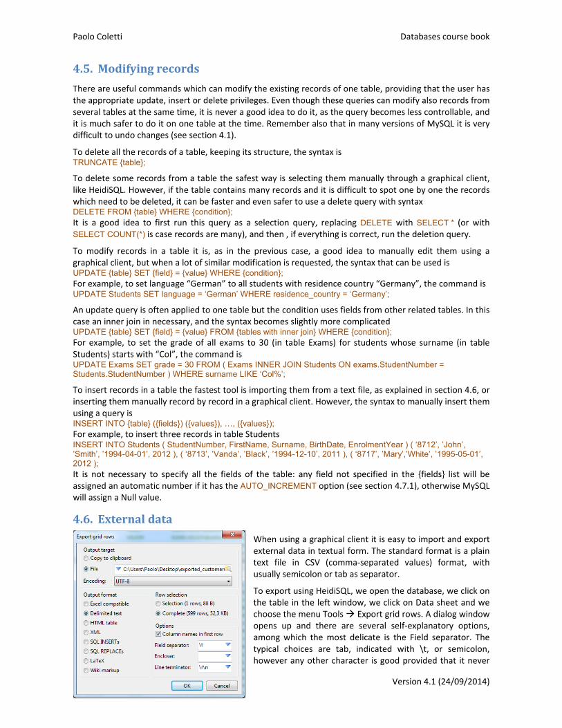
Paolo Coletti Databases course book
Page 34 of 44 Version 4.1 (24/09/2014)
4.5. Modifyingrecords
There are useful commands which can modify the existing records of one table, providing that the user has the appropriate update, insert or delete privileges. Even though these queries can modify also records from several tables at the same time, it is never a good idea to do it, as the query becomes less controllable, and it is much safer to do it on one table at the time. Remember also that in many versions of MySQL it is very difficult to undo changes (see section 4.1).
To delete all the records of a table, keeping its structure, the syntax is TRUNCATE {table};
To delete some records from a table the safest way is selecting them manually through a graphical client, like HeidiSQL. However, if the table contains many records and it is difficult to spot one by one the records which need to be deleted, it can be faster and even safer to use a delete query with syntax DELETE FROM {table} WHERE {condition}; It is a good idea to first run this query as a selection query, replacing DELETE with SELECT * (or with SELECT COUNT(*) is case records are many), and then , if everything is correct, run the deletion query.
To modify records in a table it is, as in the previous case, a good idea to manually edit them using a graphical client, but when a lot of similar modification is requested, the syntax that can be used is UPDATE {table} SET {field} = {value} WHERE {condition}; For example, to set language “German” to all students with residence country “Germany”, the command is UPDATE Students SET language = ‘German’ WHERE residence_country = ‘Germany’;
An update query is often applied to one table but the condition uses fields from other related tables. In this case an inner join in necessary, and the syntax becomes slightly more complicated UPDATE {table} SET {field} = {value} FROM {tables with inner join} WHERE {condition}; For example, to set the grade of all exams to 30 (in table Exams) for students whose surname (in table Students) starts with “Col”, the command is UPDATE Exams SET grade = 30 FROM ( Exams INNER JOIN Students ON exams.StudentNumber = Students.StudentNumber ) WHERE surname LIKE ‘Col%’;
To insert records in a table the fastest tool is importing them from a text file, as explained in section 4.6, or inserting them manually record by record in a graphical client. However, the syntax to manually insert them using a query is INSERT INTO {table} ({fields}) ({values}), …, ({values}); For example, to insert three records in table Students INSERT INTO Students ( StudentNumber, FirstName, Surname, BirthDate, EnrolmentYear ) ( ‘8712’, ’John’, ’Smith’, ’1994-04-01’, 2012 ), ( ‘8713’, ’Vanda’, ’Black’, ’1994-12-10’, 2011 ), ( ‘8717’, ’Mary’,’White’, ’1995-05-01’, 2012 ); It is not necessary to specify all the fields of the table: any field not specified in the {fields} list will be assigned an automatic number if it has the AUTO_INCREMENT option (see section 4.7.1), otherwise MySQL will assign a Null value.
4.6. Externaldata
When using a graphical client it is easy to import and export external data in textual form. The standard format is a plain text file in CSV (comma‐separated values) format, with usually semicolon or tab as separator.
To export using HeidiSQL, we open the database, we click on the table in the left window, we click on Data sheet and we choose the menu Tools Export grid rows. A dialog window opens up and there are several self‐explanatory options, among which the most delicate is the Field separator. The typical choices are tab, indicated with \t, or semicolon, however any other character is good provided that it never
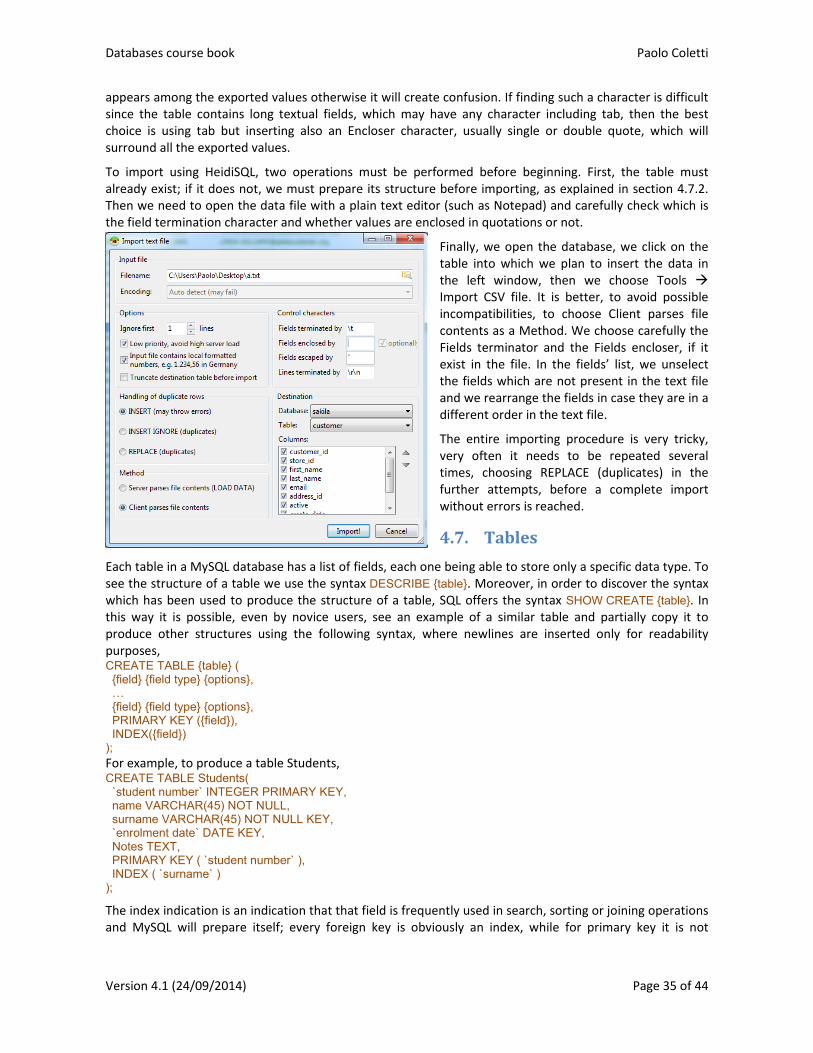
Databases course book Paolo Coletti
Version 4.1 (24/09/2014) Page 35 of 44
appears among the exported values otherwise it will create confusion. If finding such a character is difficult since the table contains long textual fields, which may have any character including tab, then the best choice is using tab but inserting also an Encloser character, usually single or double quote, which will surround all the exported values.
To import using HeidiSQL, two operations must be performed before beginning. First, the table must already exist; if it does not, we must prepare its structure before importing, as explained in section 4.7.2. Then we need to open the data file with a plain text editor (such as Notepad) and carefully check which is the field termination character and whether values are enclosed in quotations or not.
Finally, we open the database, we click on the table into which we plan to insert the data in the left window, then we choose Tools Import CSV file. It is better, to avoid possible incompatibilities, to choose Client parses file contents as a Method. We choose carefully the Fields terminator and the Fields encloser, if it exist in the file. In the fields’ list, we unselect the fields which are not present in the text file and we rearrange the fields in case they are in a different order in the text file.
The entire importing procedure is very tricky, very often it needs to be repeated several times, choosing REPLACE (duplicates) in the further attempts, before a complete import without errors is reached.
4.7. Tables
Each table in a MySQL database has a list of fields, each one being able to store only a specific data type. To see the structure of a table we use the syntax DESCRIBE {table}. Moreover, in order to discover the syntax which has been used to produce the structure of a table, SQL offers the syntax SHOW CREATE {table}. In this way it is possible, even by novice users, see an example of a similar table and partially copy it to produce other structures using the following syntax, where newlines are inserted only for readability purposes, CREATE TABLE {table} ( {field} {field type} {options}, … {field} {field type} {options}, PRIMARY KEY ({field}), INDEX({field}) ); For example, to produce a table Students, CREATE TABLE Students( `student number` INTEGER PRIMARY KEY, name VARCHAR(45) NOT NULL, surname VARCHAR(45) NOT NULL KEY, `enrolment date` DATE KEY, Notes TEXT, PRIMARY KEY ( `student number` ), INDEX ( `surname` ) );
The index indication is an indication that that field is frequently used in search, sorting or joining operations and MySQL will prepare itself; every foreign key is obviously an index, while for primary key it is not

Paolo Coletti Databases course book
Page 36 of 44 Version 4.1 (24/09/2014)
necessary to indicate it as it is implicit in the primary key indication. Concerning other fields, for some it is obvious that they must be indexes, for example field surname in every people’s table, for others the decision is up to the database designed while for some others it is evident that they are not indexes, such as fields Notes or Picture.
We can add some “check constraints” to a table to limit the possibility of wrong data insertions, adding to the syntax CHECK {condition}. For example, to admit only students with a number larger than 1000 and an enrolment date not in the future CREATE TABLE Students( `student number` INTEGER, name VARCHAR(45) NOT NULL, surname VARCHAR(45) NOT NULL KEY, `enrolment date` DATE KEY, Notes TEXT, PRIMARY KEY ( ‘student number’ ), INDEX ( `surname` ), CHECK ( `student number` >1000 ), CHECK ( `enrolment date` <=CURDATE() ) ); Unfortunately, up to version 5.6 MySQL accepts any CHECK command but does not really implement the CHECK constraint!
Even though it is never a good idea to do it (with the exception of adding other fields, a rather safe operation), to change a table structure after it has been created the following syntaxes can be used: DROP TABLE {table}; ALTER TABLE {table} ADD {field} {field type} {options}; ALTER TABLE {table} DROP {field}; ALTER TABLE {table} ADD PRIMARY KEY {field}; ALTER TABLE {table} DROP PRIMARY KEY;
4.7.1. Fieldtypes
Each field in a MySQL table must have a predefined type, according to what it is going to contain. The most frequently used types are:
INT, for a integer number from ‐2 billions up to 2 billions
TINYINT, 0 or 1, used for boolean values
DECIMAL ( {maximum total number of digits} , {number of decimal digits} ) FLOAT, for a non‐exact real number
CHAR ( {number of characters} ), for fixed length text
VARCHAR( {maximum number of characters} ), for variable length text
TEXT, for very long text up to 60,000 characters
ENUM( {value} , … , {value} ), for text values only in the indicated list (warning: numbers must be inserted as text; if ‘7’ is inserted, it is interpreted as value 7, but if 7 is inserted, it is interpreted as the 7th value of the values’ list)
DATE, for a date (time is supposed to be midnight)
DATETIME, for a date with time.
These types can have also some options, even combined together. The most important ones are:
NOT NULL, this field may never contain a Null value
AUTO_INCREMENT, this field will contain an automatically incremented numerical value whenever a new record in inserted without a specification of this field’s value
UNIQUE, this is a field for which all records must contain a different value for this field
DEFAULT {default value}, anytime a new record is inserted without specifying a value for this field, the default value will be used.
Note that the primary key field automatically has UNIQUE and NOT NULL options and is an index field.
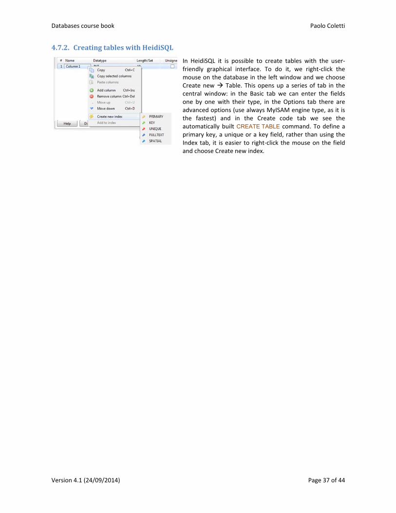
Databases course book Paolo Coletti
Version 4.1 (24/09/2014) Page 37 of 44
4.7.2. CreatingtableswithHeidiSQL
In HeidiSQL it is possible to create tables with the user‐friendly graphical interface. To do it, we right‐click the mouse on the database in the left window and we choose Create new Table. This opens up a series of tab in the central window: in the Basic tab we can enter the fields one by one with their type, in the Options tab there are advanced options (use always MyISAM engine type, as it is the fastest) and in the Create code tab we see the automatically built CREATE TABLE command. To define a primary key, a unique or a key field, rather than using the Index tab, it is easier to right‐click the mouse on the field and choose Create new index.
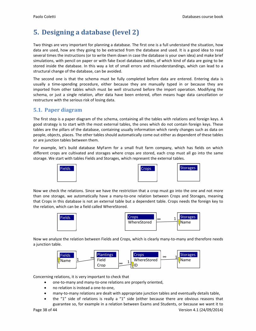
Paolo Coletti Databases course book
Page 38 of 44 Version 4.1 (24/09/2014)
5. Designingadatabase(level2)
Two things are very important for planning a database. The first one is a full understand the situation, how data are used, how are they going to be extracted from the database and used. It is a good idea to read several times the instructions (or to write them down in case the database is your own idea) and make brief simulations, with pencil on paper or with fake Excel database tables, of which kind of data are going to be stored inside the database. In this way a lot of small errors and misunderstandings, which can lead to a structural change of the database, can be avoided.
The second one is that the schema must be fully completed before data are entered. Entering data is usually a time‐spending procedure, either because they are manually typed in or because they are imported from other tables which must be well structured before the import operation. Modifying the schema, or just a single relation, after data have been entered, often means huge data cancellation or restructure with the serious risk of losing data.
5.1. Paperdiagram
The first step is a paper diagram of the schema, containing all the tables with relations and foreign keys. A good strategy is to start with the most external tables, the ones which do not contain foreign keys. These tables are the pillars of the database, containing usually information which rarely changes such as data on people, objects, places. The other tables should automatically come out either as dependent of these tables or are junction tables between them.
For example, let’s build database MyFarm for a small fruit farm company, which has fields on which different crops are cultivated and storages where crops are stored, each crop must all go into the same storage. We start with tables Fields and Storages, which represent the external tables.
Now we check the relations. Since we have the restriction that a crop must go into the one and not more than one storage, we automatically have a many‐to‐one relation between Crops and Storages, meaning that Crops in this database is not an external table but a dependent table. Crops needs the foreign key to the relation, which can be a field called WhereStored.
Now we analyze the relation between Fields and Crops, which is clearly many‐to‐many and therefore needs a junction table.
Concerning relations, it is very important to check that
one‐to‐many and many‐to‐one relations are properly oriented,
no relation is instead a one‐to‐one,
many‐to‐many relations are dealt with appropriate junction tables and eventually details table,
the “1” side of relations is really a “1” side (either because there are obvious reasons that guarantee so, for example in a relation between Exams and Students, or because we want it to
Storages
Fields
Crops
∞ 1 Storages Name
Fields
Crops WhereStored
∞
∞
11
Storages Name ∞1
Fields Name
PlantingsField Crop
CropsWhereStored ID
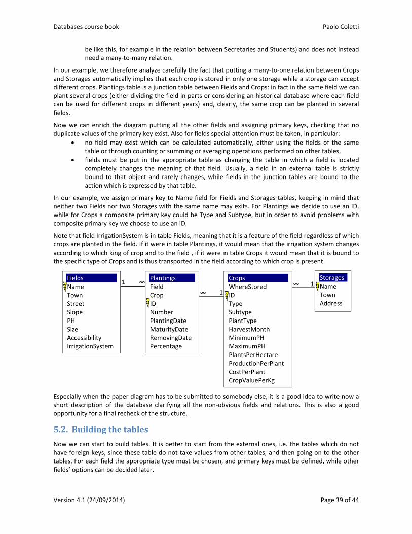
Databases course book Paolo Coletti
Version 4.1 (24/09/2014) Page 39 of 44
be like this, for example in the relation between Secretaries and Students) and does not instead need a many‐to‐many relation.
In our example, we therefore analyze carefully the fact that putting a many‐to‐one relation between Crops and Storages automatically implies that each crop is stored in only one storage while a storage can accept different crops. Plantings table is a junction table between Fields and Crops: in fact in the same field we can plant several crops (either dividing the field in parts or considering an historical database where each field can be used for different crops in different years) and, clearly, the same crop can be planted in several fields.
Now we can enrich the diagram putting all the other fields and assigning primary keys, checking that no duplicate values of the primary key exist. Also for fields special attention must be taken, in particular:
no field may exist which can be calculated automatically, either using the fields of the same table or through counting or summing or averaging operations performed on other tables,
fields must be put in the appropriate table as changing the table in which a field is located completely changes the meaning of that field. Usually, a field in an external table is strictly bound to that object and rarely changes, while fields in the junction tables are bound to the action which is expressed by that table.
In our example, we assign primary key to Name field for Fields and Storages tables, keeping in mind that neither two Fields nor two Storages with the same name may exits. For Plantings we decide to use an ID, while for Crops a composite primary key could be Type and Subtype, but in order to avoid problems with composite primary key we choose to use an ID.
Note that field IrrigationSystem is in table Fields, meaning that it is a feature of the field regardless of which crops are planted in the field. If it were in table Plantings, it would mean that the irrigation system changes according to which king of crop and to the field , if it were in table Crops it would mean that it is bound to the specific type of Crops and is thus transported in the field according to which crop is present.
Especially when the paper diagram has to be submitted to somebody else, it is a good idea to write now a short description of the database clarifying all the non‐obvious fields and relations. This is also a good opportunity for a final recheck of the structure.
5.2. Buildingthetables
Now we can start to build tables. It is better to start from the external ones, i.e. the tables which do not have foreign keys, since these table do not take values from other tables, and then going on to the other tables. For each field the appropriate type must be chosen, and primary keys must be defined, while other fields’ options can be decided later.
∞
∞
1 1
Storages Name Town Address
∞1 Fields Name Town Street Slope PH Size Accessibility IrrigationSystem
PlantingsField Crop ID Number PlantingDate MaturityDate RemovingDate Percentage
CropsWhereStored ID Type Subtype PlantType HarvestMonth MinimumPH MaximumPH PlantsPerHectare ProductionPerPlant CostPerPlant CropValuePerKg

Paolo Coletti Databases course book
Page 40 of 44 Version 4.1 (24/09/2014)
For example, in the previous database:
for table Fields: o Name, Town, and Street contain text (text for Access; VARCHAR(30) VARCHAR(50) VARCHAR(50) for
MySQL); o Slope, MinimumPH, MaximumPH and Size contain numbers (number for Access; DECIMAL(4,2)
DECIMAL(3,2) INTEGER for MySQL); o Accessibility and IrrigationSystem contain yes/no (yes/no for Access; ENUM(‘yes’,’no’) or INTEGER for
Mysql);
for table Storages: Name, Town, and Address contain text (text for Access; VARCHAR(30) VARCHAR(50)
VARCHAR(50) for MySQL).
for table Crops: o ID is an automatic incrementing number (autonumber for Access, INTEGER with AUTO_INCREMENT
for MySQL); o Type, Subtype, Plant Type contain text (text for Access; VARCHAR(30) VARCHAR(30) VARCHAR(10)
for MySQL); o HarvestMonth can contain text (text for Access; VARCHAR(9) or ENUM(‘January’, …, ’December’) for
MySQL) or number (number for Access; INTEGER for MySQL); o MinimumPH, MaximumPH, PlantsPerHectare, ProductionPerPlant, CostPerPlant, and
CropValuePerKg contain numbers (number for Access; DECIMAL(3,2) DECIMAL(3,2) INTEGER FLOAT
DECIMAL(6,2) FLOAT for MySQL);
for table Plantings: o ID is an automatic incrementing number (autonumber for Access, INTEGER with AUTO_INCREMENT
for MySQL); o Number (number for Access; INTEGER for MySQL); o Percentage contain numbers (number, single with 2 decimal digits and percentage format, for Access;
DECIMAL(5,2) for MySQL) o PlantingDate, MaturityDate, and RemovingDate are dates (date/time for Access, DATE for MySQL).
Foreign keys must be set in MySQL to the same type of the corresponding primary key.
Foreign keys can be set in Access
to the same type of the corresponding primary key and then the relation can be built in the relationships diagram, remembering to enforce referential integrity;
as Lookup Wizard type choosing as displayed values the appropriate meaningful fields from the related table, hiding the primary key when it is an ID (and thus not meaningful for a human operator) or unhiding it when it is meaningful. Then referential integrity is enforced in the relationships diagram.
5.2.1. Fieldoptions
Once fields are defined we can set also all the options. For example, in the Plantings table:
Field and Crops have the required (NOT NULL in MySQL) option;
Number has validation rule >=0 and a validation text “Number of planted plants must be zero or positive” (in MYSQL condition CHECK Number>=0);
PlantingDate is set as required (NON NULL in MySQL) and we set also the option index duplicates allowed (set it as index in MySQL) since we are going to do searches based on the PlantingDate;
MaturityDate and RemovingDate are not set to required since we want to leave the possibility to have these fields empty (for example, if we do not know when we will remove this planting);
fields Town in table Fields, Type and SubType in table Crops and Town in table Storages are set as Index Duplicates OK (INDEX in MySQL), because we imagine they will be frequently used for sorting and filtering by the user. Automatically all primary keys are also set to the same option;
Percentage has validation rule Between 0 And 1 and validation text “Percentage of used field must be between 0% and 100%” (in MySQL condition CHECK (Percentage BETWEEN 0 AND 1)). We can also set
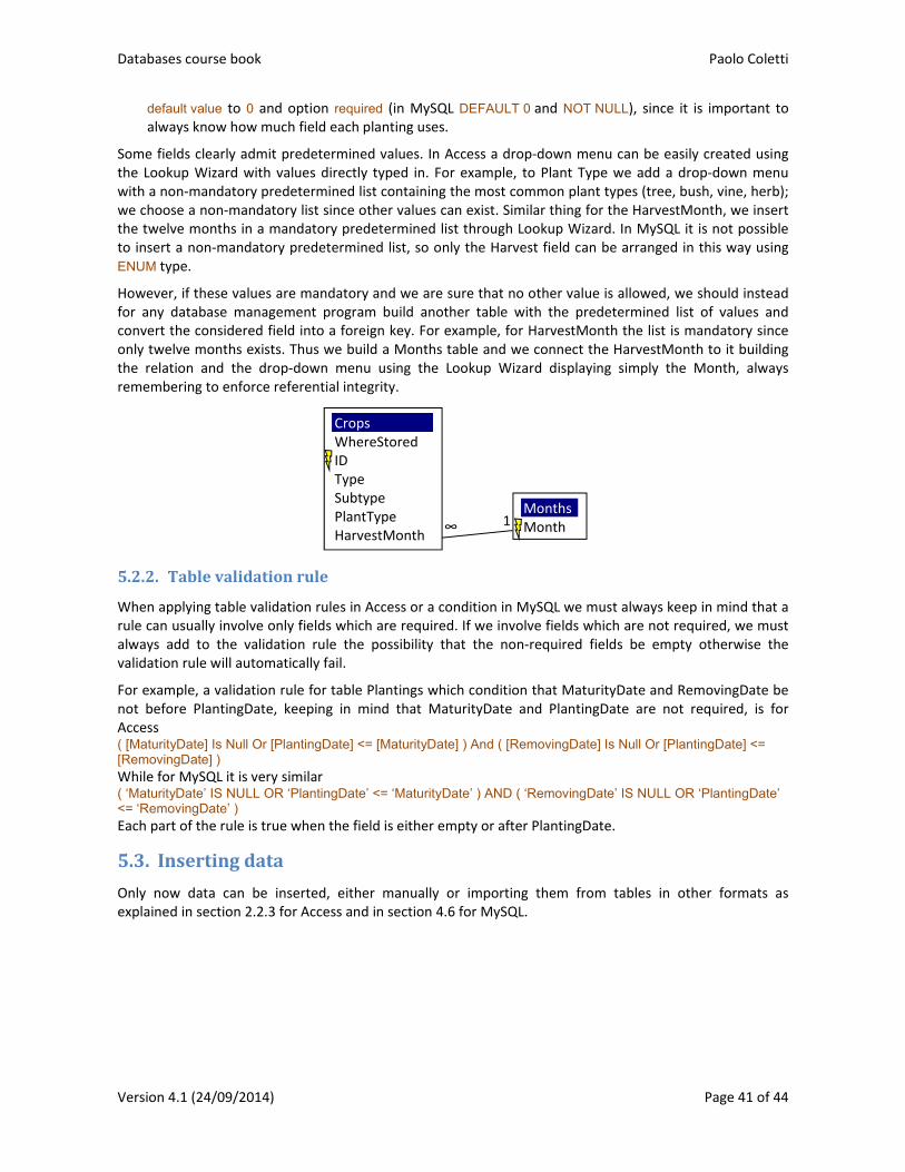
Databases course book Paolo Coletti
Version 4.1 (24/09/2014) Page 41 of 44
default value to 0 and option required (in MySQL DEFAULT 0 and NOT NULL), since it is important to always know how much field each planting uses.
Some fields clearly admit predetermined values. In Access a drop‐down menu can be easily created using the Lookup Wizard with values directly typed in. For example, to Plant Type we add a drop‐down menu with a non‐mandatory predetermined list containing the most common plant types (tree, bush, vine, herb); we choose a non‐mandatory list since other values can exist. Similar thing for the HarvestMonth, we insert the twelve months in a mandatory predetermined list through Lookup Wizard. In MySQL it is not possible to insert a non‐mandatory predetermined list, so only the Harvest field can be arranged in this way using ENUM type.
However, if these values are mandatory and we are sure that no other value is allowed, we should instead for any database management program build another table with the predetermined list of values and convert the considered field into a foreign key. For example, for HarvestMonth the list is mandatory since only twelve months exists. Thus we build a Months table and we connect the HarvestMonth to it building the relation and the drop‐down menu using the Lookup Wizard displaying simply the Month, always remembering to enforce referential integrity.
5.2.2. Tablevalidationrule
When applying table validation rules in Access or a condition in MySQL we must always keep in mind that a rule can usually involve only fields which are required. If we involve fields which are not required, we must always add to the validation rule the possibility that the non‐required fields be empty otherwise the validation rule will automatically fail.
For example, a validation rule for table Plantings which condition that MaturityDate and RemovingDate be not before PlantingDate, keeping in mind that MaturityDate and PlantingDate are not required, is for Access ( [MaturityDate] Is Null Or [PlantingDate] <= [MaturityDate] ) And ( [RemovingDate] Is Null Or [PlantingDate] <= [RemovingDate] ) While for MySQL it is very similar ( ‘MaturityDate’ IS NULL OR ‘PlantingDate’ <= ‘MaturityDate’ ) AND ( ‘RemovingDate’ IS NULL OR ‘PlantingDate’ <= ‘RemovingDate’ ) Each part of the rule is true when the field is either empty or after PlantingDate.
5.3. Insertingdata
Only now data can be inserted, either manually or importing them from tables in other formats as explained in section 2.2.3 for Access and in section 4.6 for MySQL.
∞ 1
Crops WhereStored ID Type Subtype PlantType HarvestMonth
MonthsMonth
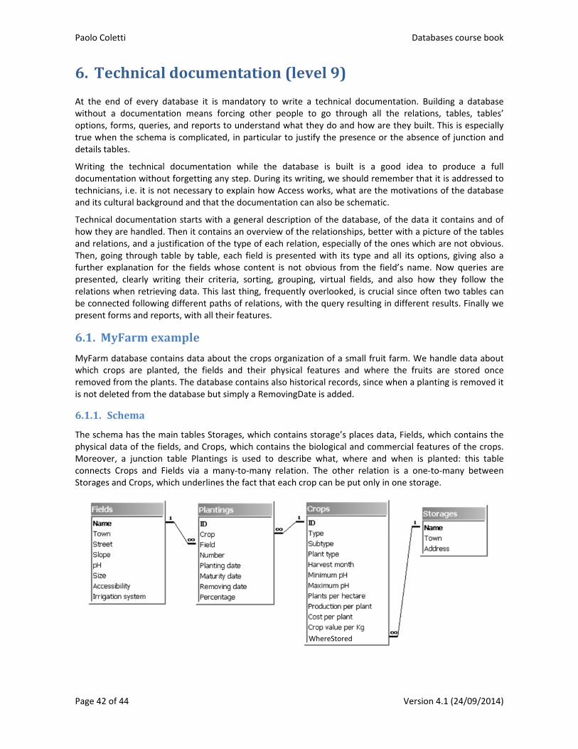
Paolo Coletti Databases course book
Page 42 of 44 Version 4.1 (24/09/2014)
6. Technicaldocumentation(level9)
At the end of every database it is mandatory to write a technical documentation. Building a database without a documentation means forcing other people to go through all the relations, tables, tables’ options, forms, queries, and reports to understand what they do and how are they built. This is especially true when the schema is complicated, in particular to justify the presence or the absence of junction and details tables.
Writing the technical documentation while the database is built is a good idea to produce a full documentation without forgetting any step. During its writing, we should remember that it is addressed to technicians, i.e. it is not necessary to explain how Access works, what are the motivations of the database and its cultural background and that the documentation can also be schematic.
Technical documentation starts with a general description of the database, of the data it contains and of how they are handled. Then it contains an overview of the relationships, better with a picture of the tables and relations, and a justification of the type of each relation, especially of the ones which are not obvious. Then, going through table by table, each field is presented with its type and all its options, giving also a further explanation for the fields whose content is not obvious from the field’s name. Now queries are presented, clearly writing their criteria, sorting, grouping, virtual fields, and also how they follow the relations when retrieving data. This last thing, frequently overlooked, is crucial since often two tables can be connected following different paths of relations, with the query resulting in different results. Finally we present forms and reports, with all their features.
6.1. MyFarmexample
MyFarm database contains data about the crops organization of a small fruit farm. We handle data about which crops are planted, the fields and their physical features and where the fruits are stored once removed from the plants. The database contains also historical records, since when a planting is removed it is not deleted from the database but simply a RemovingDate is added.
6.1.1. Schema
The schema has the main tables Storages, which contains storage’s places data, Fields, which contains the physical data of the fields, and Crops, which contains the biological and commercial features of the crops. Moreover, a junction table Plantings is used to describe what, where and when is planted: this table connects Crops and Fields via a many‐to‐many relation. The other relation is a one‐to‐many between Storages and Crops, which underlines the fact that each crop can be put only in one storage.
WhereStored

Databases course book Paolo Coletti
Version 4.1 (24/09/2014) Page 43 of 44
6.1.2. Tablesandfields
Warning: field types are for Access. For MySQL they must be properly adapted.
Table Fields contains Name: text, primary key; Town, Street: text; Slope, pH, Size: number; Accessibility: yes/no. This indicates whether a road arrives to the field; IrrigationSystem: yes/no, required, default value no.
Table Storages contains Name: text, primary key; Town, Address: text;
Table Crops contains ID: autonumber, primary key; Type, HarvestMonth: text; Plant type: text. This contains the plant type such as tree, bush or herb. Subtype: text. This contains the specific type of fruit, for example Pear Kaiser, Apple Golden; MinimumPH, MaximumPH, PlantsPerHectare, ProductionPerPlant: number; CostPerPlant, CropValuePerKg: currency; WhereStored: foreign key, takes values from Storages table.
Table Plantings contains ID: autonumber, primary key; Crop: foreign key, takes values from Crops table. Field: foreign key, takes values from Fields table. Number: number. This indicates how many plants of Crop type are planted in Field; PlantingDate, MaturityDate, RemovingDate: date/time; Percentage: number. This indicates which percentage of the field is used for this crop.
6.1.3. Tablesandfieldswithoptions
Warning: field options are for Access. For MySQL they must be properly adapted.
Table Fields contains Name: text limited to 50 characters, primary key, required, no zero length; Town, Street: text limited to 50 characters; Slope: number, integer with 0 decimal digits, default value 0; MinimumPH and MaximumPH: number, single with 2 decimal digits, default value 5, must be between
0 and 10; Size: number, single with 2 decimal digits, default value 0, must be positive; Accessibility: yes/no. This field indicates whether a road arrives to the field; IrrigationSystem: yes/no, required, default value no.
Table Storages contains Name: text limited to 50 characters, primary key, required, no zero length; Town, Address: text limited to 50 characters;
Table Crops contains ID: autonumber, primary key; Type: text limited to 50 characters, required, no zero length text, indexed (with duplicates), non‐
mandatory predetermined list with values Apple, Pear, Strawberry, Grapevine;

Paolo Coletti Databases course book
Page 44 of 44 Version 4.1 (24/09/2014)
Subtype: text limited to 50 characters, required. This contains the specific type of fruit, for example Pear Kaiser, Apple Golden;
Plant type: text limited to 50 characters, non‐mandatory predetermined list with values Tree, Bush, Vine, Herb;
HarvestMonth: text limited to 50 characters, non‐mandatory predetermined list with the twelve months as values, there is an extra table Months, containing the twelve months, for which this field is a foreign key;
MinimumPH, MaximumPH: number, single with 2 decimal digits, required, default value 5, must be between 0 and 10;
PlantsPerHectare: number, integer with 0 decimal digits, default value 0, must be positive; ProductionPerPlant: number, single with 2 decimal digits, default value 0, must be non‐negative; CostPerPlant: currency, euro format, single with 2 decimal digits, default value 0; CropValuePerKg: currency, euro format, single with 2 decimal digits, default value 0; WhereStored: foreign key, takes values from Storages table.
Table Plantings contains ID: autonumber, primary key; Crop: foreign key, takes values from Crops table. Field: foreign key, takes values from Fields table. Number: number, integer with 0 decimal digits, default value 0, must be non‐negative. This field
indicates how many plants of Crop type are planted in Field; PlantingDate: date/time, format dd/mm/yyyy, required, indexed (duplicates allowed); MaturityDate, RemovingDate: date/time, format dd/mm/yyyy; Percentage: number, percentage format, single with 2 decimal digits, default value 0%, must be
between 0% and 100%. This indicates which percentage of the field is used for this crop. To table Plantings there is also a table validation rule that checks that MaturityDate and RemovingDate, when they exist, are not before PlantingDate.
6.1.4. Forms
Form Insert/Modify Crops shows the crops with their storage, using the relation between Storages and Crops. It is possible to modify them or to insert new ones, but deletion of crops is forbidden.
6.1.5. Queries
Query Type+Subtype+Field Without Irrigation Query shows the field without an IrrigationSystem with the crop type and crop subtype that are and were planted in that field. This query retrieves the fields with a No in the IrrigationSystem field and then, thanks to the junction table Plantings and following the two relations, retrieves the crop’s type and subtype.
6.1.6. ReportsReport Crops by Harvest Month displays, grouped by HarvestMonth and then grouped by crop type, the crop subtype and the corresponding field and town where the crop is or was planted. It takes data from tables Crops and Fields, connected through the junction table Plantings and the two relations.


![Presentazione prof maurizio coletti [modalità compatibilità]](https://img.pdfslide.net/doc/110x75/5592ec8a1a28ab7e408b46ff/presentazione-prof-maurizio-coletti-modalita-compatibilita.jpg)