Embed Size (px)
Citation preview
Datalogging Experiments.
Properties of Solutions :Electrolytes and Non-Electrolytes
Conductivity of Solutions: The Effect of Concentration
Evaporation and Intermolecular Attractions
Titration Curves of Strong and Weak Acids and Bases
Boyle’s Law: Pressure-Volume Relationship in Gases
Determining the Concentration of a Solution: Beer’s Law
Pressure-Temperature Relationship in Gases
A Good Cold Pack
Rusting
The Electrochemical Series
Properties of Solutions: Electrolytes and Non-Electrolytes
In this experiment, you will discover some properties of strong electrolytes, weak electrolytes, and
non-electrolytes by observing the behavior of these substances in aqueous solutions. You will
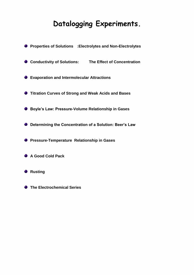
determine these properties using a Conductivity Probe. When the probe is placed in a solution that
contains ions, and thus has the ability to conduct electricity, an electrical circuit is completed across
the electrodes that are located on either side of the hole near the bottom of the probe body (see
Figure 1). This results in a conductivity value that can be read by LabQuest. The unit of
conductivity used in this experiment is the microsiemens per centimeter, or µS/cm.
The size of the conductivity value depends on the ability of the aqueous solution
to conduct electricity. Strong electrolytes produce large numbers of ions,
which results in high conductivity values. Weak electrolytes result in low
conductivity, and non-electrolytes should result in no conductivity. In this
experiment, you will observe several factors that determine whether or not
a solution conducts, and if so, the relative magnitude of the
conductivity. Thus, this simple experiment allows you to learn a great deal
about different compounds and their resulting solutions.
In each part of the experiment, you will be observing a different
property of electrolytes. Keep in mind that you will be
encountering three types of compounds and aqueous
solutions:
Ionic Compounds
These are usually strong electrolytes and can be expected to 100% dissociate in aqueous solution.
Example: NaNO3(s) Na+(aq) + NO3–(aq)
Molecular Compounds
These are usually non-electrolytes. They do not dissociate to form ions. Resulting solutions do not conduct electricity.
Example: CH3OH(l) CH3OH(aq)
Molecular Acids
These are molecules that can partially or wholly dissociate, depending on their strength.
Example: Strong electrolyte H2SO4 H+(aq) + HSO4–(aq) (100% dissociation)
Example: Weak electrolyte HF H+(aq) + F–(aq) (<100% dissociation)

MATERIALS
PROCEDURE
1. Obtain and wear goggles! DANGER: Handle all the solutions in this experiment with care.
They may be harmful if swallowed or in contact with the skin or eyes. Do not handle until all
safety precautions have been understood
2. Assemble the Conductivity Probe, utility clamp, and ring stand as shown in Figure 1. Be sure
the probe is clean and dry before beginning the experiment.
3. Set the selector switch on the side of the Conductivity Probe to the 0–20000 µS/cm range.
Connect the Conductivity Probe to LabQuest and choose New from the File menu. If you have
an older sensor that does not auto-ID, manually set up the sensor.
4. Obtain the Group A solution containers. The solutions are: 0.05 M CaCl2, 0.05 M NaCl, and
0.05 M AlCl3.
5. Measure the conductivity of each of the solutions.
a. Carefully raise each vial and its contents up around the Conductivity Probe until the hole
near the probe end is completely submerged in the solution being tested. Important: Since
the two electrodes are positioned on either side of the hole, this part of the probe must be
completely submerged.
b. Briefly swirl the vial contents. Monitor the conductivity reading displayed on the screen for
6–8 seconds, then record the value in your data table.
c. Before testing the next solution, clean the electrodes by surrounding them with a 250 mL
beaker and rinse them with distilled water from a wash bottle. Blot the outside of the probe
end dry using a tissue. It is not necessary to dry the inside of the hole near the probe end.
LabQuest 0.05 M NaCl A
LabQuest App 0.05 M CaCl2 A
Vernier Conductivity Probe 0.05 M AlCl3 A
Ring stand 0.05 M HC2H3O2 B
Utility clamp 0.05 M H3PO4 B
250 mL beaker 0.05 M H3BO3 B
Wash bottle and distilled water 0.05 M HCl B
Tissues 0.05 M CH3OH (methanol) C H2O (tap) C 0.05 M C2H6O2 (ethylene glycol) C
H2O (distilled) C
6. Obtain the four Group B solution containers. These include 0.05 M HC2H3O2, 0.05 M HCl,
0.05 M H3PO4, and 0.05 M H3BO3. Repeat the Step 5 procedure.
7. Obtain the five Group C solutions or liquids. These include distilled H2O, tap H2O,
0.05 M CH3OH, and 0.05 M C2H6O2. Repeat the Step 5 procedure.
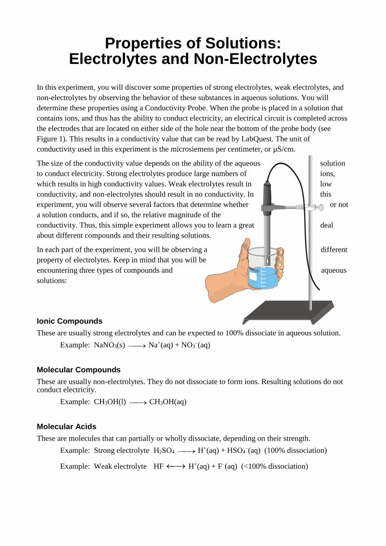
RESULTS.
Solution Conductivity (µS/cm)
A - CaCl2
A - AlCl3
A - NaCl
B - HC2H3O2
B - HCl
B - H3PO4
B - H3BO3
C - H2Odistilled
C - H2Otap
C - CH3OH
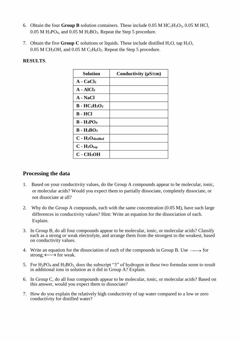
Processing the data
1. Based on your conductivity values, do the Group A compounds appear to be molecular, ionic,
or molecular acids? Would you expect them to partially dissociate, completely dissociate, or
not dissociate at all?
2. Why do the Group A compounds, each with the same concentration (0.05 M), have such large
differences in conductivity values? Hint: Write an equation for the dissociation of each.
Explain.
3. In Group B, do all four compounds appear to be molecular, ionic, or molecular acids? Classify each as a strong or weak electrolyte, and arrange them from the strongest to the weakest, based on conductivity values.
4. Write an equation for the dissociation of each of the compounds in Group B. Use for strong;
for weak.
5. For H3PO4 and H3BO3, does the subscript “3” of hydrogen in these two formulas seem to result in additional ions in solution as it did in Group A? Explain.
6. In Group C, do all four compounds appear to be molecular, ionic, or molecular acids? Based on this answer, would you expect them to dissociate?
7. How do you explain the relatively high conductivity of tap water compared to a low or zero conductivity for distilled water?
Conductivity of Solutions: The Effect of Concentration
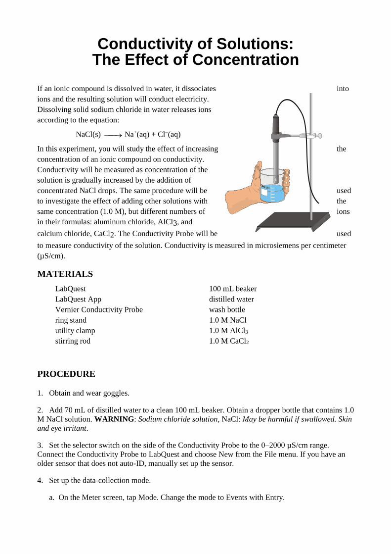
If an ionic compound is dissolved in water, it dissociates into
ions and the resulting solution will conduct electricity.
Dissolving solid sodium chloride in water releases ions
according to the equation:
NaCl(s) Na+(aq) + Cl–(aq)
In this experiment, you will study the effect of increasing the
concentration of an ionic compound on conductivity.
Conductivity will be measured as concentration of the
solution is gradually increased by the addition of
concentrated NaCl drops. The same procedure will be used
to investigate the effect of adding other solutions with the
same concentration (1.0 M), but different numbers of ions
in their formulas: aluminum chloride, AlCl3, and
calcium chloride, CaCl2. The Conductivity Probe will be used
to measure conductivity of the solution. Conductivity is measured in microsiemens per centimeter
(µS/cm).
MATERIALS
LabQuest 100 mL beaker
LabQuest App distilled water
Vernier Conductivity Probe wash bottle
ring stand 1.0 M NaCl
utility clamp 1.0 M AlCl3
stirring rod 1.0 M CaCl2
PROCEDURE
1. Obtain and wear goggles.
2. Add 70 mL of distilled water to a clean 100 mL beaker. Obtain a dropper bottle that contains 1.0
M NaCl solution. WARNING: Sodium chloride solution, NaCl: May be harmful if swallowed. Skin
and eye irritant.
3. Set the selector switch on the side of the Conductivity Probe to the 0–2000 µS/cm range.
Connect the Conductivity Probe to LabQuest and choose New from the File menu. If you have an
older sensor that does not auto-ID, manually set up the sensor.
4. Set up the data-collection mode.
a. On the Meter screen, tap Mode. Change the mode to Events with Entry.
b. Enter the Name (Volume) and Units (drops). Select OK.
5. Before adding any drops of solution:
a. Start data collection.
b. Carefully raise the beaker and its contents up around the Conductivity Probe until the hole
near the probe end is completely submerged in the solution being tested. Important: Since
the two electrodes are positioned on either side of the hole, this part of the probe must be
completely submerged.
c. Before you have added any drops of NaCl solution, tap Keep. Enter 0, the volume (in drops)
and then select OK to save this data pair for this experiment.
d. Lower the beaker away from the probe.
6. You are now ready to begin adding salt solution.
a. Add 1 drop of NaCl solution to the distilled water. Stir to ensure thorough mixing.
b. Carefully raise the beaker and its contents up around the Conductivity Probe until the hole
near the probe end is completely submerged in the solution being tested.
c. Briefly swirl the beaker contents. Monitor the conductivity of the solution for about
5 seconds.
d. When the conductivity readings stabilize, tap Keep. Enter 1 as the volume in drops and then
select OK. The conductivity and volume values have now been saved for the second trial.
e. Lower the beaker away from the probe.
7. Repeat the Step 6 procedure, entering 2 this time.
8. Continue this procedure, adding 1-drop portions of NaCl solution, measuring conductivity, and
entering the total number of drops added—until a total of 8 drops has been added.
9. Stop data collection.
10. To analyze the relationship between conductivity and volume, use this method to calculate
the linear-regression statistics for your data. Then plot the linear regression curve on your graph.
a. Choose Curve Fit from the Analyze menu.
b. Select Linear for the Fit Equation. Note: Since increasing the volume (drops) of NaCl
increases the concentration of NaCl in the solution, the graph actually represents the
relationship between conductivity and concentration. The linear-regression statistics for these
two lists are displayed for the equation in the form
bmxy
where y is conductivity, x is volume, m is the slope, and b is the y-intercept.
c. Record the value for the slope, m, in your data table.
d. Select OK.
11. Store the data from the first run by tapping the File Cabinet icon.
12. Repeat Steps 5–11, this time using 1.0 M AlCl3 solution in place of 1.0 M NaCl solution.
WARNING: Aluminum chloride solution, AlCl3: May be harmful if swallowed. Causes skin and
eye irritation.
13. Repeat Steps 5–10, this time using 1.0 M CaCl2 solution. WARNING: Calcium chloride
solution, CaCl2: May be harmful if swallowed. Causes skin and eye irritation. Important: Do not
store this run as you did in the first two runs—proceed directly to Step 14 after you complete Step
10.
14. To view a graph of concentration vs. volume showing all three data runs, tap Run 3 and
select All Runs. All three runs will now be displayed on the same graph axes.
15. (optional) Print a copy of the graph displayed in Step 14. Label each run as “1.0 M NaCl,”
“1.0 M AlCl3,” or “1.0 M CaCl2.”
Processing the data
1. Describe the appearance of each of the three curves on your graph in Step 14.
2. Describe the change in conductivity as the concentration of the NaCl solution was increased by
the addition of NaCl drops. What kind of mathematical relationship does there appear to be between
conductivity and concentration?
3. Write a chemical equation for the dissociation of NaCl, AlCl3, and CaCl2 in water.
4. Which graph had the largest slope value? The smallest? Since all solutions had the same
original concentration (1.0 M), what accounts for the difference in the slope of the three plots?
Explain.
DATA TABLE
Solution Slope, m
1.0 M NaCl
1.0 M AlCl3
1.0 M CaCl2
Evaporation and Intermolecular Attractions
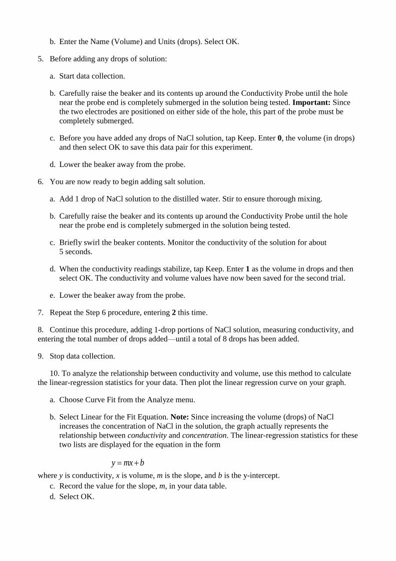
In this experiment, Temperature Probes are placed in various liquids. Evaporation occurs when the
probe is removed from the liquid’s container. This evaporation is an endothermic process that
results in a temperature decrease. The magnitude of a temperature decrease is, like viscosity and
boiling temperature, related to the strength of intermolecular forces of attraction. In this experiment,
you will study temperature changes caused by the evaporation of several liquids and relate the
temperature changes to the strength of intermolecular forces of attraction. You will use the results to
predict, and then measure, the temperature change for several other liquids.
You will encounter two types of organic compounds in this experiment—alkanes and alcohols. The
two alkanes are pentane, C5H12, and hexane, C6H14. In addition to carbon and hydrogen atoms,
alcohols also contain the -OH functional group. Methanol, CH3OH, and ethanol, C2H5OH, are two
of the alcohols that we will use in this experiment. You will examine the molecular structure of
alkanes and alcohols for the presence and relative strength of two intermolecular forces—hydrogen
bonding and dispersion forces. You will also use this experiment to compare the temperature
changes for propan-1-ol (mol. Wt = 60) and propanone (mol. Wt =59) and determine which has the
greater intermolecular forces.
MATERIALS
LabQuest methanol (methyl alcohol)
LabQuest App ethanol (ethyl alcohol)
2 Temperature Probes 1-propanol
6 pieces of filter paper (2.5 cm X 2.5 cm) 1-butanol
2 small rubber bands n-pentane
masking tape n-hexane
propanone
Pre-lab exercise
Prior to doing the experiment, complete the Pre-Lab table. The name and formula are given for each
compound. Draw a structural formula for a molecule of each compound. Then determine the
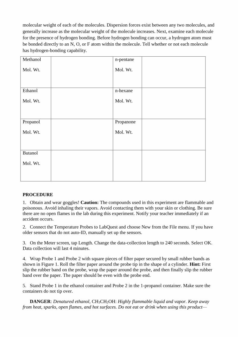
molecular weight of each of the molecules. Dispersion forces exist between any two molecules, and
generally increase as the molecular weight of the molecule increases. Next, examine each molecule
for the presence of hydrogen bonding. Before hydrogen bonding can occur, a hydrogen atom must
be bonded directly to an N, O, or F atom within the molecule. Tell whether or not each molecule
has hydrogen-bonding capability.
Methanol
Mol. Wt.
n-pentane
Mol. Wt.
Ethanol
Mol. Wt.
n-hexane
Mol. Wt.
Propanol
Mol. Wt.
Propanone
Mol. Wt.
Butanol
Mol. Wt.
PROCEDURE
1. Obtain and wear goggles! Caution: The compounds used in this experiment are flammable and
poisonous. Avoid inhaling their vapors. Avoid contacting them with your skin or clothing. Be sure
there are no open flames in the lab during this experiment. Notify your teacher immediately if an
accident occurs.
2. Connect the Temperature Probes to LabQuest and choose New from the File menu. If you have
older sensors that do not auto-ID, manually set up the sensors.
3. On the Meter screen, tap Length. Change the data-collection length to 240 seconds. Select OK.
Data collection will last 4 minutes.
4. Wrap Probe 1 and Probe 2 with square pieces of filter paper secured by small rubber bands as
shown in Figure 1. Roll the filter paper around the probe tip in the shape of a cylinder. Hint: First
slip the rubber band on the probe, wrap the paper around the probe, and then finally slip the rubber
band over the paper. The paper should be even with the probe end.
5. Stand Probe 1 in the ethanol container and Probe 2 in the 1-propanol container. Make sure the
containers do not tip over.
DANGER: Denatured ethanol, CH3CH2OH: Highly flammable liquid and vapor. Keep away
from heat, sparks, open flames, and hot surfaces. Do not eat or drink when using this product—
harmful if swallowed. Causes skin and serious eye irritation. May cause respiratory irritation.
Avoid breathing mist, vapors or spray. Causes damage to organs. Addition of denaturant makes the
product poisonous. Cannot be made nonpoisonous.
DANGER: 1-Propanol: Keep away from heat, sparks, open flames, and hot surfaces—highly
flammable liquid and vapor. Do not eat or drink when using this product—harmful if swallowed.
Causes mild skin irritation and serious eye damage. May be harmful if inhaled. May cause
drowsiness or dizziness.
6. Prepare 2 pieces of masking tape, each about 10 cm long, to be used to tape the probes in
position during Step 7.
7. After the probes have been in the liquids for at least 30 seconds, start data collection. A live
graph of temperature vs. time for both Probe 1 and Probe 2 is being plotted on the screen. Live
readings are displayed to the right of the graph. Monitor the temperature for 15 seconds to establish
the initial temperature of each liquid. Then simultaneously remove the probes from the liquids and
tape them so the probe tips extend 5 cm over the edge of the table top as shown in Figure 1.
8. Data collection will stop after 4 minutes (or stop data collection before 4 minutes has elapsed).
Examine the graph of temperature vs. time. Based on your data, determine the maximum
temperature, t1, and minimum temperature, t2 for both probes. Record t1 and t2 for each probe.
9. For each liquid, subtract the minimum temperature from the maximum temperature to determine
t, the temperature change during evaporation.
10. Based on the t values you obtained for these two substances, plus information in the
Pre-Lab exercise, predict the size of the t value for 1-butanol. Compare its hydrogen-bonding
capability and molecular weight to those of ethanol and 1-propanol. Record your predicted t, then
explain how you arrived at this answer in the space provided. Do the same for n-pentane. It is not
important that you predict the exact t value; simply estimate a logical value that is higher, lower,
or between the previous t values.
11. Test your prediction in Step 10 by repeating Steps 5–9 using 1-butanol with Probe 1 and n-
pentane with Probe 2.
DANGER: 1-Butanol, C4H9OH: Keep away from heat, sparks, open flames, and hot
surfaces—highly flammable liquid and vapor. Toxic if swallowed, in contact with skin, or if inhaled.
Do not eat or drink when using this product. Do not breath mist, vapors, or spray. Causes skin and
serious eye irritation. Causes damage to organs.
DANGER: n-Pentane, CH3(CH2)3CH3: Keep away from heat, sparks, open flames, and hot
surfaces—highly flammable liquid and vapor. Do not eat or drink when using this product—
harmful if swallowed or in contact with skin. Avoid breathing mist, vapors or spray. May cause
drowsiness or dizziness.
12. Based on the t values you have obtained for all four substances, plus information in the
Pre-Lab exercise, predict the t values for methanol and n-hexane. Compare the hydrogen-bonding
capability and molecular weight of methanol and n-hexane to those of the previous four liquids.
Record your predicted t, then explain how you arrived at this answer in the space provided.
13. Test your prediction in Step 12 by repeating Steps 5–9, using methanol with Probe 1 and n-
hexane with Probe 2.
DANGER: Methanol, CH3OH: Keep away from heat, sparks, open flames, and hot
surfaces—highly flammable liquid and vapor. Toxic if swallowed, in contact with skin, or if inhaled.
Do not eat or drink when using this product. Do not breath mist, vapors, or spray. Causes skin and
serious eye irritation. Causes damage to organs.
DANGER: n-Hexane, C6H14: Keep away from heat, sparks, open flames, and hot surfaces—
highly flammable liquid and vapor. Do not eat or drink when using this product. Avoid breathing
mist, vapors, or spray. May be fatal if swallowed and enters airways. May cause damage to organs.
Causes skin and eye irritation. May cause drowsiness or dizziness. Suspected of damaging fertility
or the unborn child. Do not handle until all safety precautions have been understood.
14 Repeat steps 5 – 9 using propanol with Probe 1 and propanone with Probe 2
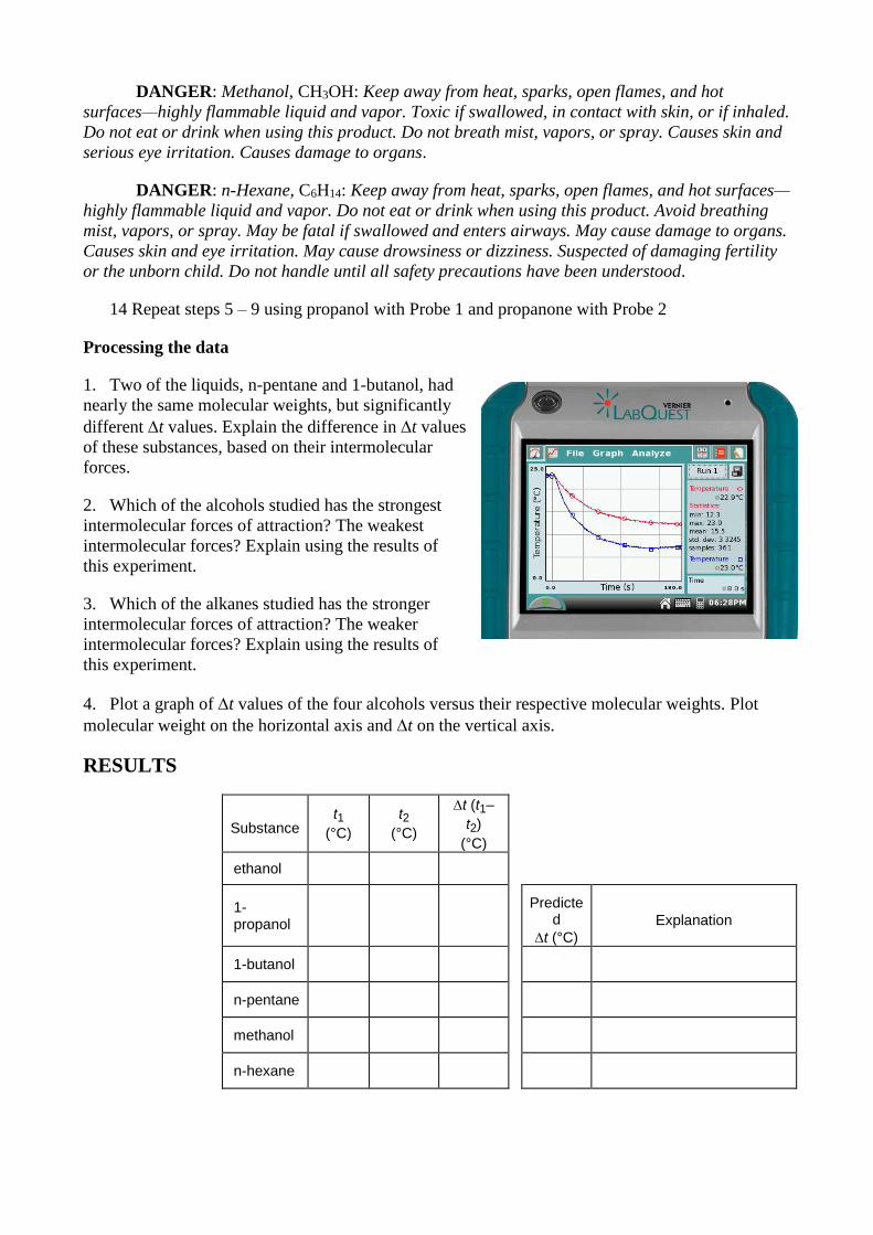
Processing the data
1. Two of the liquids, n-pentane and 1-butanol, had
nearly the same molecular weights, but significantly
different t values. Explain the difference in t values
of these substances, based on their intermolecular
forces.
2. Which of the alcohols studied has the strongest
intermolecular forces of attraction? The weakest
intermolecular forces? Explain using the results of
this experiment.
3. Which of the alkanes studied has the stronger
intermolecular forces of attraction? The weaker
intermolecular forces? Explain using the results of
this experiment.
4. Plot a graph of t values of the four alcohols versus their respective molecular weights. Plot
molecular weight on the horizontal axis and t on the vertical axis.
RESULTS
Substance t1
(°C)
t2
(°C)
t (t1–
t2)
(°C)
ethanol
1-propanol
Predicted
t (°C)
Explanation
1-butanol
n-pentane
methanol
n-hexane
Titration Curves of Strong and Weak Acids and Bases
In this experiment you will react the following combinations of strong and weak acids and bases:
Hydrochloric acid, HCl (strong acid), with sodium hydroxide, NaOH (strong base)
Hydrochloric acid, HCl (strong acid), with ammonia, NH3 (weak base)
Acetic acid, HC2H3O2 (weak acid), with sodium hydroxide, NaOH (strong base)
Acetic acid, HC2H3O2 (weak acid), with ammonia, NH3 (weak base)
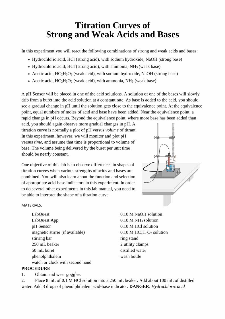
A pH Sensor will be placed in one of the acid solutions. A solution of one of the bases will slowly
drip from a buret into the acid solution at a constant rate. As base is added to the acid, you should
see a gradual change in pH until the solution gets close to the equivalence point. At the equivalence
point, equal numbers of moles of acid and base have been added. Near the equivalence point, a
rapid change in pH occurs. Beyond the equivalence point, where more base has been added than
acid, you should again observe more gradual changes in pH. A
titration curve is normally a plot of pH versus volume of titrant.
In this experiment, however, we will monitor and plot pH
versus time, and assume that time is proportional to volume of
base. The volume being delivered by the buret per unit time
should be nearly constant.
One objective of this lab is to observe differences in shapes of
titration curves when various strengths of acids and bases are
combined. You will also learn about the function and selection
of appropriate acid-base indicators in this experiment. In order
to do several other experiments in this lab manual, you need to
be able to interpret the shape of a titration curve.
MATERIALS.
LabQuest 0.10 M NaOH solution
LabQuest App 0.10 M NH3 solution
pH Sensor 0.10 M HCl solution
magnetic stirrer (if available) 0.10 M HC2H3O2 solution
stirring bar ring stand
250 mL beaker 2 utility clamps
50 mL buret distilled water
phenolphthalein wash bottle
watch or clock with second hand
PROCEDURE
1. Obtain and wear goggles.
2. Place 8 mL of 0.1 M HCl solution into a 250 mL beaker. Add about 100 mL of distilled
water. Add 3 drops of phenolphthalein acid-base indicator. DANGER: Hydrochloric acid
solution, HCl: Causes severe skin and eye damage. Do not breathe mist, vapors, or spray. May
cause respiratory irritation. May be harmful if swallowed.
3. Place the beaker onto a magnetic stirrer and add a small stirring bar.
4. Connect the pH Sensor to LabQuest and choose New from the File menu. If you have an
older sensor that does not auto-ID, manually set up the sensor.
5. Use a utility clamp to suspend a pH Sensor on a ring stand as shown in Figure 1. Situate the
pH Sensor in the HCl solution and adjust its position toward the outside of the beaker so that it is
not struck by the stirring bar.
6. Obtain a 50 mL buret and rinse the buret with a few mL of the 0.1 M NaOH solution. Fill
the buret to about the 0 mL mark. WARNING: Sodium hydroxide solution, NaOH: Causes skin and
eye irritation.
7. On the Meter screen, tap Length. Change the data-collection length to 240 seconds. Select
OK. Data collection will last 4 minutes.
8. You are now ready to begin monitoring data. Note: To determine the elapsed time when the
indicator changes color in Step 9, monitor the time (in seconds) on a clock as soon as you start data
collection.
Start data collection. Carefully open the burette stopcock to provide a dripping rate of about
1 drop per second. Do not worry if the rate is somewhat faster or slower when you first start; initial
additions of base will have very little effect on the pH.
9. Watch to see if the phenolphthalein changes color before, at the same time, or after the rapid
change in pH at the equivalence point. If phenolphthalein is a suitable indicator for this reaction, it
should change from clear to red at about the same time as the jump in pH occurs. In your data table,
record the elapsed time when the phenolphthalein color change occurs.
10. When data collection stops after 4 minutes, turn the buret stopcock to stop the flow
of NaOH titrant. As you tap each data point, the pH and time values are displayed to the right of the
graph. Determine the approximate time for the equivalence point; that is, for the biggest jump in pH
in the steep vertical region of the curve. Record this time in the data table. Rinse the pH Sensor and
return it to the pH storage solution. Dispose of the beaker contents as directed by your teacher.
Clean and dry the 250 mL beaker for the next trial.
11. Before printing the graph of pH vs. time, rescale the y axis from 0 to 14 pH units.
a. Choose Graph Option from the Graph menu.
b. Enter 14 as the Graph 1 Y-Axis Top value.
c. Enter 0 as the Graph 1 Y-Axis Bottom value.
d. Select OK. The y-axis on the displayed graph should now have pH scaled from 0 to 14.
12. Print a graph of pH vs. time. Label the graph with the acid and base used for the
reaction.
13. Repeat the procedure using NaOH titrant and acetic acid solution, HC2H3O2. You do
not need to refill the buret. Add 8 mL of 0.10 M HC2H3O2 solution to the 250 mL beaker. Add
about 100 mL of distilled water and 3 drops of phenolphthalein to the beaker. Rinse the tip of the
pH Sensor and position it in the acid solution as you did in Step 5. Repeat the data collection using
Steps 8–12 of the procedure.
14. Repeat the procedure using NH3 titrant and HCl solution. DANGER: Ammonia,
NH3: Causes skin irritation and serious eye damage. Drain the remaining NaOH from the buret and
dispose of it as directed by your teacher. Rinse the 50-mL buret with a few mL of the 0.1 M NH3
solution. Fill the buret with NH3 solution to about the 0-mL mark. Add 8 mL of 0.10 M HCl
solution to the 250 mL beaker. Add about 100 mL of distilled water and 3 drops of phenolphthalein
to the beaker. Rinse the sensor and position it in the acid solution as you did in Step 5. Repeat the
data collection using Steps 8–12 of the procedure.
15. Repeat the procedure using NH3 titrant and HC2H3O2 solution. \You do not need to
refill the buret. Add 8 mL of 0.10 M HC2H3O2 solution to the 250 mL beaker. Add about 100 mL of
distilled water and 3 drops of phenolphthalein to the beaker. Rinse the pH Sensor and position it in
the acid solution as you did in Step 5. Repeat the data collection using Steps 8–12 of the procedure.
16. When you are finished, rinse the pH Sensor with distilled water and return it to the
pH storage solution.
Processing the data
1. Examine the time data for each of the Trials 1–4. In which trial(s) did the indicator change
color at about the same time as the large increase in pH occurred at the equivalence point? In which
trial(s) was there a significant difference in these two times?
2. Phenolphthalein changes from clear to red at a pH value of about 9. According to your
results, with which combination(s) of strong or weak acids and bases can phenolphthalein be used
to determine the equivalence point?
3. On each of the four graphs, draw a horizontal line from a pH value of 9 on the vertical axis
to its intersection with the titration curve. In which trial(s) does this line intersect the nearly vertical
region of the curve? In which trial(s) does this line miss the nearly vertical region of the curve?
4. Compare your answers to Questions 1 and 3. By examining a titration curve, how can you
decide which acid-base indicator to use to find the equivalence point?
5. Methyl red is an acid-base indicator that changes color at a pH value of about 5. From what
you learned in this lab, methyl red could be used to determine the equivalence point of what
combination of strong or weak acids and bases?
6. Of the four titration curves, which combination of strong or weak acids and bases had the
longest vertical region of the equivalence point? The shortest?
7. The acid-base reaction between HCl and NaOH produces a solution with a pH of 7 at the
equivalence point (NaCl + H2O). Why does an acid-base indicator that changes color at pH 5 or 9
work just as well for this reaction as one that changes color at pH 7?
8. In general, how does the shape of a curve with a weak specie (NH3 or HC2H3O2) differ from
the shape of a curve with a strong specie (NaOH or HCl)?
9. Complete each of the equations in the table below.
RESULTS:
Trial Equation for acid-base reaction Time of indicator
color change Time at
equivalence point
1 NaOH + HCl s s
2 NaOH + HC2H3O2 s s
3 NH3 + HCl s s
4 NH3 + HC2H3O2 s s
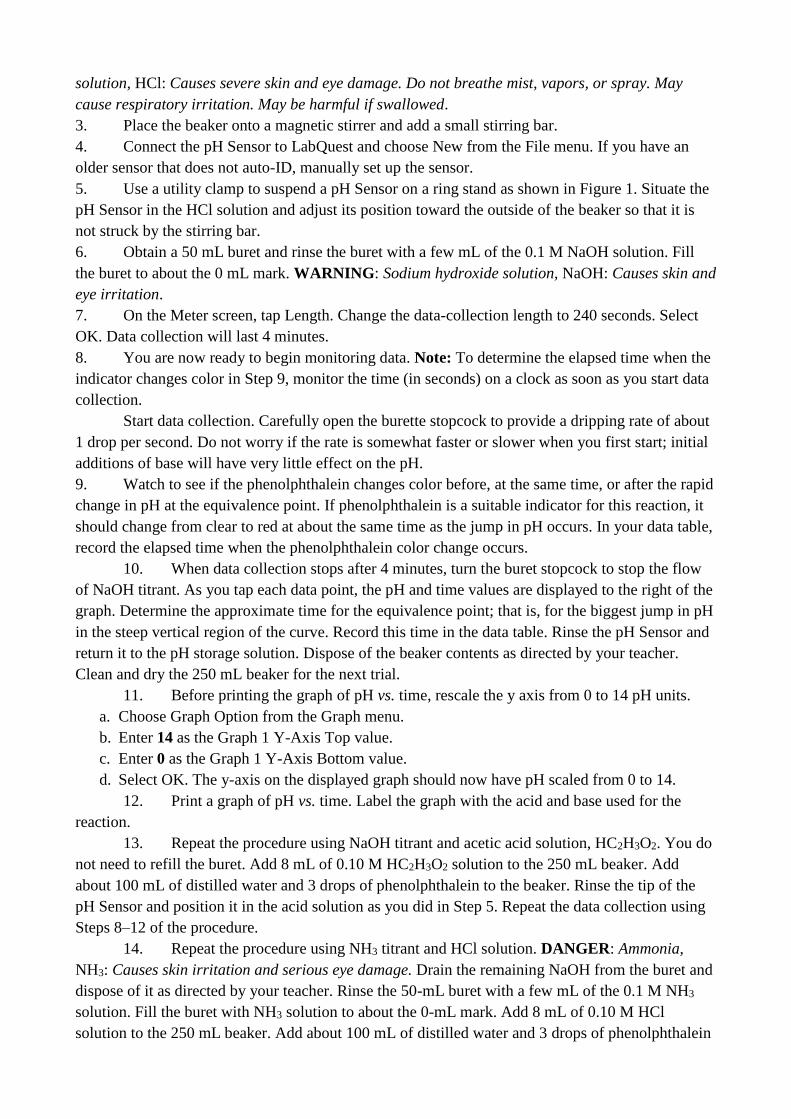
An alternate way of determining the precise equivalence point of the titration is to take the first and
second derivatives of the pH-volume data.
1. Determine the peak value on the first derivative
vs. time plot.
a. Tap the Table tab. Choose New Calculated
Column from the Table menu.
b. Enter d1 as the Calculated Column Name. Select
the equation, 1st derivative (Y,X). Use Time as
the Column for X, and pH as the Column for Y.
Select OK.
c. On the displayed plot of d1 vs. time, examine the
graph to determine the time at the peak value of
the first derivative.
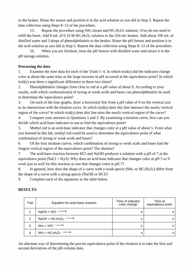
2. Determine the zero value on the second
derivative vs. time plot.
a. Tap the Table tab. Choose New Calculated
Column from the Table menu.
b. Enter d2 as the Calculated Column Name. Select
the equation, 2nd derivative (Y,X). Use Time as
the Column for X, and pH as the Column for Y.
Select OK.
c. On the displayed plot of d2 vs. time, examine the
graph to determine the volume when the 2nd
derivative equals approximately zero.
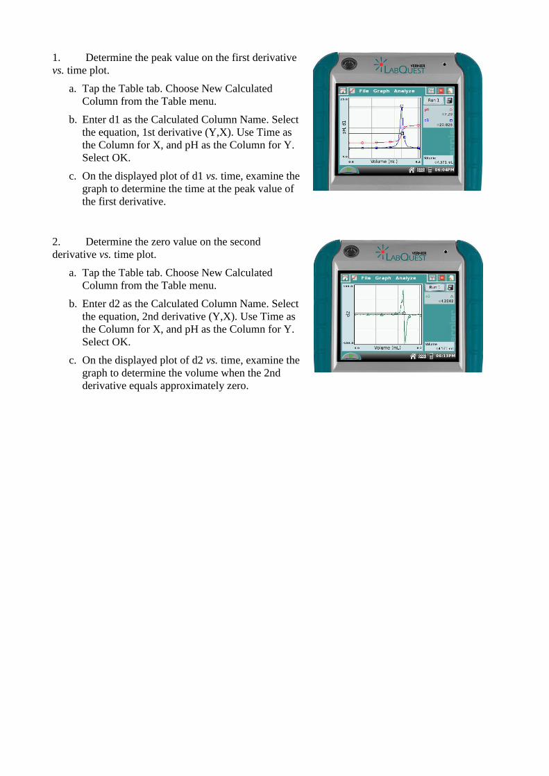
Boyle’s Law: Pressure-Volume Relationship in Gases
The primary objective of this experiment is to determine the relationship between the pressure and
volume of a confined gas. The gas we use will be air, and it will be confined in a syringe connected
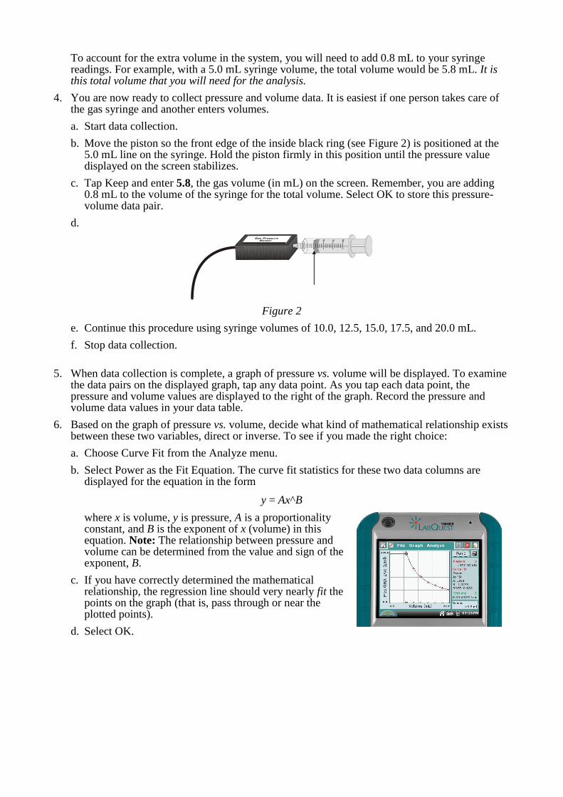
to a Gas Pressure Sensor (see Figure 1). When the volume of the syringe is changed by moving the
piston, a change occurs in the pressure exerted by the confined gas. This pressure change will be
monitored using a Gas Pressure Sensor. It is assumed that temperature will be constant throughout
the experiment. Pressure and volume data pairs will be collected during this experiment and then
analyzed. From the data and graph, you should be able to determine what kind of mathematical
relationship exists between the pressure and volume of the confined gas. Historically, this
relationship was first established by Robert Boyle in 1662 and has since been known as Boyle’s
law.
MATERIALS
LabQuest Vernier Gas Pressure Sensor
LabQuest App 20 mL gas syringe
PROCEDURE
1. Prepare the Gas Pressure Sensor and an air sample for data collection.
a. Connect the Gas Pressure Sensor to LabQuest and choose New from the File menu. If you have an older sensor that does not auto-ID, manually set up the sensor.
b. With the 20 mL syringe disconnected from the Gas Pressure Sensor, move the piston of the syringe until the front edge of the inside black ring (indicated by the arrow in Figure 1) is positioned at the 10.0 mL mark.
c. Attach the 20 mL syringe to the valve of the Gas Pressure Sensor.
2. Set up the data-collection mode.
a. On the Meter screen, tap Mode. Change the mode to Events with Entry.
b. Enter the Name (Volume) and Units (mL). Select OK.
3. To obtain the best data possible, you will need to correct the volume readings from the syringe. Look at the syringe; its scale reports its own internal volume. However, that volume is not the total volume of trapped air in your system since there is a little bit of space inside the pressure sensor.
To account for the extra volume in the system, you will need to add 0.8 mL to your syringe readings. For example, with a 5.0 mL syringe volume, the total volume would be 5.8 mL. It is this total volume that you will need for the analysis.
4. You are now ready to collect pressure and volume data. It is easiest if one person takes care of the gas syringe and another enters volumes.
a. Start data collection.
b. Move the piston so the front edge of the inside black ring (see Figure 2) is positioned at the 5.0 mL line on the syringe. Hold the piston firmly in this position until the pressure value displayed on the screen stabilizes.
c. Tap Keep and enter 5.8, the gas volume (in mL) on the screen. Remember, you are adding 0.8 mL to the volume of the syringe for the total volume. Select OK to store this pressure-volume data pair.
d.
Figure 2
e. Continue this procedure using syringe volumes of 10.0, 12.5, 15.0, 17.5, and 20.0 mL.
f. Stop data collection.
5. When data collection is complete, a graph of pressure vs. volume will be displayed. To examine the data pairs on the displayed graph, tap any data point. As you tap each data point, the pressure and volume values are displayed to the right of the graph. Record the pressure and volume data values in your data table.
6. Based on the graph of pressure vs. volume, decide what kind of mathematical relationship exists between these two variables, direct or inverse. To see if you made the right choice:
a. Choose Curve Fit from the Analyze menu.
b. Select Power as the Fit Equation. The curve fit statistics for these two data columns are displayed for the equation in the form
y = Ax^B
where x is volume, y is pressure, A is a proportionality constant, and B is the exponent of x (volume) in this equation. Note: The relationship between pressure and volume can be determined from the value and sign of the exponent, B.
c. If you have correctly determined the mathematical relationship, the regression line should very nearly fit the points on the graph (that is, pass through or near the plotted points).
d. Select OK.
RESULTS
Volume (mL)
Pressure (kPa)
Constant, k (P / V or P • V)
PROCESSING THE DATA
1. If the volume is doubled from 5.0 mL to 10.0 mL, what does your data show happens to the pressure? Show the pressure values in your answer.
2. If the volume is halved from 20.0 mL to 10.0 mL, what does your data show happens to the pressure? Show the pressure values in your answer.
3. If the volume is tripled from 5.0 mL to 15.0 mL, what does your data show happened to the pressure? Show the pressure values in your answer.
4. From your answers to the first three questions and the shape of the curve in the plot of pressure versus volume, do you think the relationship between the pressure and volume of a confined gas is direct or inverse? Explain your answer.
5. Based on your data, what would you expect the pressure to be if the volume of the syringe was increased to 40.0 mL. Explain or show work to support your answer.
6. Based on your data, what would you expect the pressure to be if the volume of the syringe was decreased to 2.5 mL.
7. What experimental factors are assumed to be constant in this experiment?
8. One way to determine if a relationship is inverse or direct is to find a proportionality constant, k, from the data. If this relationship is direct, k = P/V. If it is inverse, k = P•V. Based on your answer to Question 4, choose one of these formulas and calculate k for the seven ordered pairs in your data table (divide or multiply the P and V values). Show the answers in the third column of the Data and Calculations table.
9. How constant were the values for k you obtained in Question 8? Good data may show some minor variation, but the values for k should be relatively constant.
10. Using P, V, and k, write an equation representing Boyle’s law. Write a verbal statement that correctly expresses Boyle’s law.
EXTENSION
1. To confirm that an inverse relationship exists between pressure and volume, a graph of pressure vs. reciprocal of volume (1/volume) may also be plotted. To do this using LabQuest:
a. Tap the Table tab to display the data table.
b. Choose New Calculated Column from the Table menu.
c. Enter the Name (1/Volume) and Units (1/mL). Select the equation, A/X. Use Pressure as the Column for X, and 1 as the value for A.
d. Select OK.
2. Follow this procedure to calculate regression statistics and to plot a best-fit regression line on your graph of pressure vs. 1/volume:
a. Choose Graph Options from the Graph menu.
b. Select Autoscale from 0 and select OK.
c. Choose Curve Fit from the Analyze menu.
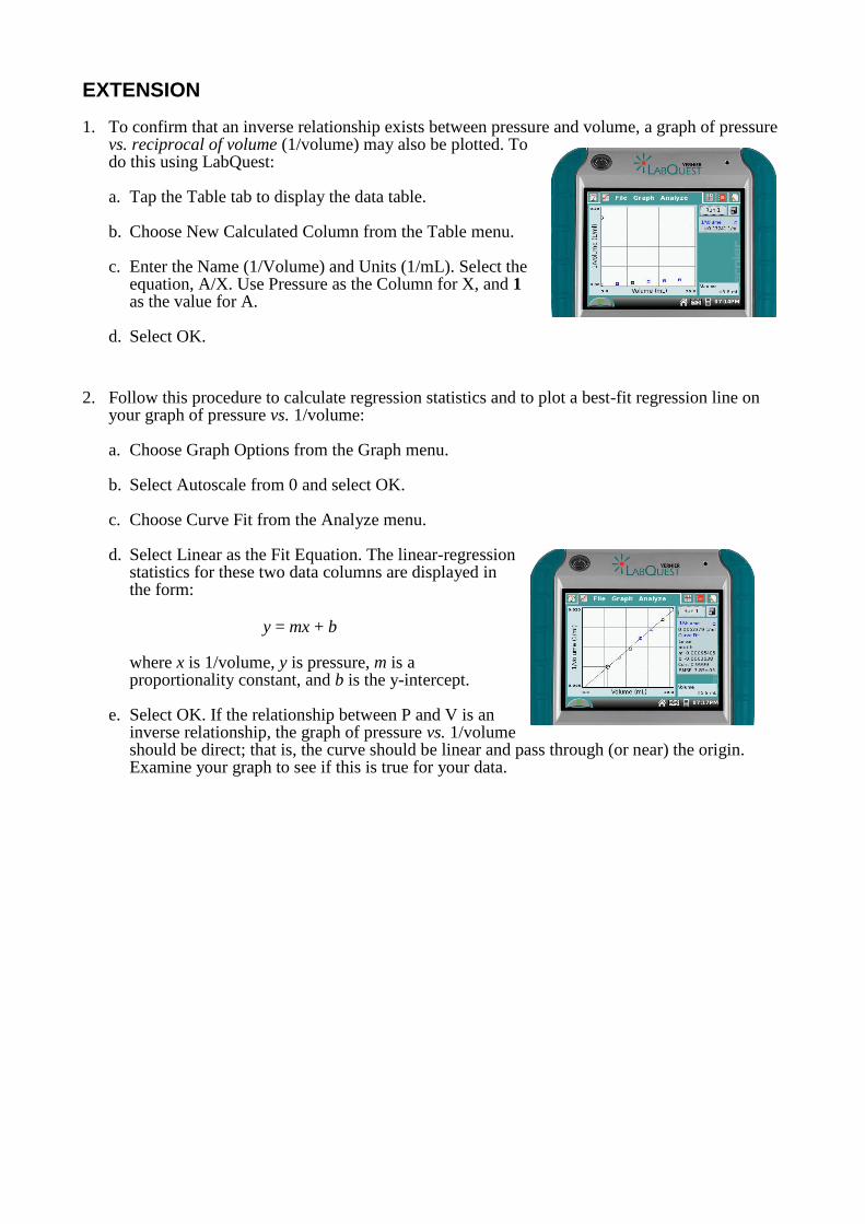
d. Select Linear as the Fit Equation. The linear-regression statistics for these two data columns are displayed in the form:
y = mx + b
where x is 1/volume, y is pressure, m is a proportionality constant, and b is the y-intercept.
e. Select OK. If the relationship between P and V is an inverse relationship, the graph of pressure vs. 1/volume should be direct; that is, the curve should be linear and pass through (or near) the origin. Examine your graph to see if this is true for your data.
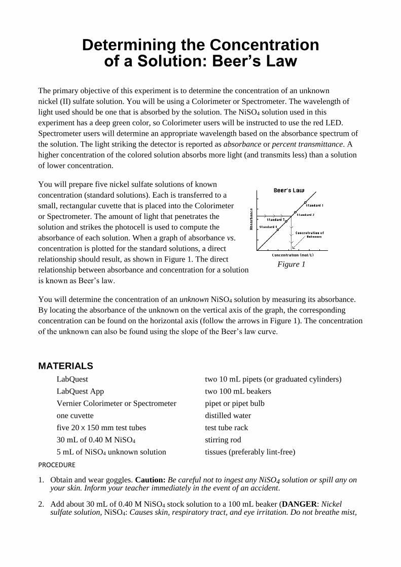
Figure 1
Determining the Concentration of a Solution: Beer’s Law
The primary objective of this experiment is to determine the concentration of an unknown
nickel (II) sulfate solution. You will be using a Colorimeter or Spectrometer. The wavelength of
light used should be one that is absorbed by the solution. The NiSO4 solution used in this
experiment has a deep green color, so Colorimeter users will be instructed to use the red LED.
Spectrometer users will determine an appropriate wavelength based on the absorbance spectrum of
the solution. The light striking the detector is reported as absorbance or percent transmittance. A
higher concentration of the colored solution absorbs more light (and transmits less) than a solution
of lower concentration.
You will prepare five nickel sulfate solutions of known
concentration (standard solutions). Each is transferred to a
small, rectangular cuvette that is placed into the Colorimeter
or Spectrometer. The amount of light that penetrates the
solution and strikes the photocell is used to compute the
absorbance of each solution. When a graph of absorbance vs.
concentration is plotted for the standard solutions, a direct
relationship should result, as shown in Figure 1. The direct
relationship between absorbance and concentration for a solution
is known as Beer’s law.
You will determine the concentration of an unknown NiSO4 solution by measuring its absorbance.
By locating the absorbance of the unknown on the vertical axis of the graph, the corresponding
concentration can be found on the horizontal axis (follow the arrows in Figure 1). The concentration
of the unknown can also be found using the slope of the Beer’s law curve.
MATERIALS
LabQuest two 10 mL pipets (or graduated cylinders)
LabQuest App two 100 mL beakers
Vernier Colorimeter or Spectrometer pipet or pipet bulb
one cuvette distilled water
five 20 X 150 mm test tubes test tube rack
30 mL of 0.40 M NiSO4 stirring rod
5 mL of NiSO4 unknown solution tissues (preferably lint-free)
PROCEDURE
1. Obtain and wear goggles. Caution: Be careful not to ingest any NiSO4 solution or spill any on your skin. Inform your teacher immediately in the event of an accident.
2. Add about 30 mL of 0.40 M NiSO4 stock solution to a 100 mL beaker (DANGER: Nickel sulfate solution, NiSO4: Causes skin, respiratory tract, and eye irritation. Do not breathe mist,
vapors, or spray—toxic if swallowed.). Add about 30 mL of distilled water to another 100 mL beaker.
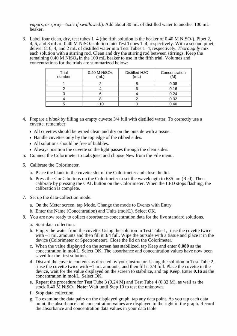
3. Label four clean, dry, test tubes 1–4 (the fifth solution is the beaker of 0.40 M NiSO4). Pipet 2, 4, 6, and 8 mL of 0.40 M NiSO4 solution into Test Tubes 1–4, respectively. With a second pipet, deliver 8, 6, 4, and 2 mL of distilled water into Test Tubes 1–4, respectively. Thoroughly mix each solution with a stirring rod. Clean and dry the stirring rod between stirrings. Keep the remaining 0.40 M NiSO4 in the 100 mL beaker to use in the fifth trial. Volumes and concentrations for the trials are summarized below:
Trial number
0.40 M NiSO4 (mL)
Distilled H2O (mL)
Concentration (M)
1 2 8 0.08
2 4 6 0.16
3 6 4 0.24
4 8 2 0.32
5 ~10 0 0.40
4. Prepare a blank by filling an empty cuvette 3/4 full with distilled water. To correctly use a cuvette, remember:
All cuvettes should be wiped clean and dry on the outside with a tissue.
Handle cuvettes only by the top edge of the ribbed sides.
All solutions should be free of bubbles.
Always position the cuvette so the light passes through the clear sides.
5. Connect the Colorimeter to LabQuest and choose New from the File menu.
6. Calibrate the Colorimeter.
a. Place the blank in the cuvette slot of the Colorimeter and close the lid.
b. Press the < or > buttons on the Colorimeter to set the wavelength to 635 nm (Red). Then calibrate by pressing the CAL button on the Colorimeter. When the LED stops flashing, the calibration is complete.
7. Set up the data-collection mode.
a. On the Meter screen, tap Mode. Change the mode to Events with Entry.
b. Enter the Name (Concentration) and Units (mol/L). Select OK.
8. You are now ready to collect absorbance-concentration data for the five standard solutions.
a. Start data collection.
b. Empty the water from the cuvette. Using the solution in Test Tube 1, rinse the cuvette twice with ~1 mL amounts and then fill it 3/4 full. Wipe the outside with a tissue and place it in the device (Colorimeter or Spectrometer). Close the lid on the Colorimeter.
c. When the value displayed on the screen has stabilized, tap Keep and enter 0.080 as the concentration in mol/L. Select OK. The absorbance and concentration values have now been saved for the first solution.
d. Discard the cuvette contents as directed by your instructor. Using the solution in Test Tube 2, rinse the cuvette twice with ~1 mL amounts, and then fill it 3/4 full. Place the cuvette in the device, wait for the value displayed on the screen to stabilize, and tap Keep. Enter 0.16 as the concentration in mol/L. Select OK.
e. Repeat the procedure for Test Tube 3 (0.24 M) and Test Tube 4 (0.32 M), as well as the stock 0.40 M NiSO4. Note: Wait until Step 10 to test the unknown.
f. Stop data collection.
g. To examine the data pairs on the displayed graph, tap any data point. As you tap each data point, the absorbance and concentration values are displayed to the right of the graph. Record the absorbance and concentration data values in your data table.
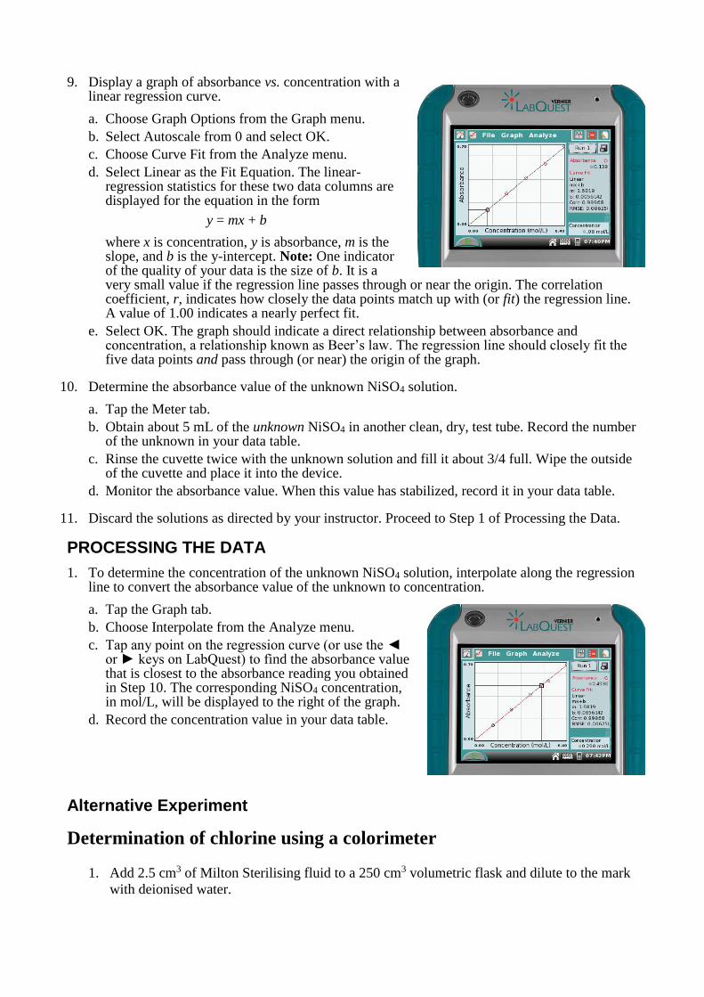
9. Display a graph of absorbance vs. concentration with a
linear regression curve.
a. Choose Graph Options from the Graph menu.
b. Select Autoscale from 0 and select OK.
c. Choose Curve Fit from the Analyze menu.
d. Select Linear as the Fit Equation. The linear-regression statistics for these two data columns are displayed for the equation in the form
y = mx + b
where x is concentration, y is absorbance, m is the slope, and b is the y-intercept. Note: One indicator of the quality of your data is the size of b. It is a very small value if the regression line passes through or near the origin. The correlation coefficient, r, indicates how closely the data points match up with (or fit) the regression line. A value of 1.00 indicates a nearly perfect fit.
e. Select OK. The graph should indicate a direct relationship between absorbance and concentration, a relationship known as Beer’s law. The regression line should closely fit the five data points and pass through (or near) the origin of the graph.
10. Determine the absorbance value of the unknown NiSO4 solution.
a. Tap the Meter tab.
b. Obtain about 5 mL of the unknown NiSO4 in another clean, dry, test tube. Record the number of the unknown in your data table.
c. Rinse the cuvette twice with the unknown solution and fill it about 3/4 full. Wipe the outside of the cuvette and place it into the device.
d. Monitor the absorbance value. When this value has stabilized, record it in your data table.
11. Discard the solutions as directed by your instructor. Proceed to Step 1 of Processing the Data.
PROCESSING THE DATA
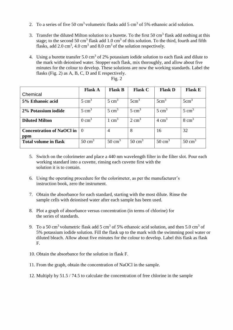
1. To determine the concentration of the unknown NiSO4 solution, interpolate along the regression line to convert the absorbance value of the unknown to concentration.
a. Tap the Graph tab.
b. Choose Interpolate from the Analyze menu.
c. Tap any point on the regression curve (or use the ◄ or ► keys on LabQuest) to find the absorbance value that is closest to the absorbance reading you obtained in Step 10. The corresponding NiSO4 concentration, in mol/L, will be displayed to the right of the graph.
d. Record the concentration value in your data table.
Alternative Experiment
Determination of chlorine using a colorimeter
1. Add 2.5 cm3 of Milton Sterilising fluid to a 250 cm3 volumetric flask and dilute to the mark
with deionised water.
2. To a series of five 50 cm3 volumetric flasks add 5 cm3 of 5% ethanoic acid solution.
3. Transfer the diluted Milton solution to a burette. To the first 50 cm3 flask add nothing at this
stage; to the second 50 cm3 flask add 1.0 cm3 of this solution. To the third, fourth and fifth
flasks, add 2.0 cm3, 4.0 cm3 and 8.0 cm3 of the solution respectively.
4. Using a burette transfer 5.0 cm3 of 2% potassium iodide solution to each flask and dilute to
the mark with deionised water. Stopper each flask, mix thoroughly, and allow about five
minutes for the colour to develop. These solutions are now the working standards. Label the
flasks (Fig. 2) as A, B, C, D and E respectively.
Fig. 2
Chemical Flask A Flask B Flask C Flask D Flask E
5% Ethanoic acid 5 cm3 5 cm3 5cm3 5cm3 5cm3
2% Potassium iodide 5 cm3 5 cm3 5 cm3 5 cm3 5 cm3
Diluted Milton 0 cm3 1 cm3 2 cm3 4 cm3 8 cm3
Concentration of NaOCl in
ppm
0 4 8 16 32
Total volume in flask 50 cm3 50 cm3 50 cm3 50 cm3 50 cm3
5. Switch on the colorimeter and place a 440 nm wavelength filter in the filter slot. Pour each
working standard into a cuvette, rinsing each cuvette first with the
solution it is to contain.
6. Using the operating procedure for the colorimeter, as per the manufacturer’s
instruction book, zero the instrument.
7. Obtain the absorbance for each standard, starting with the most dilute. Rinse the
sample cells with deionised water after each sample has been used.
8. Plot a graph of absorbance versus concentration (in terms of chlorine) for
the series of standards.
9. To a 50 cm3 volumetric flask add 5 cm3 of 5% ethanoic acid solution, and then 5.0 cm3 of
5% potassium iodide solution. Fill the flask up to the mark with the swimming pool water or
diluted bleach. Allow about five minutes for the colour to develop. Label this flask as flask
F.
10. Obtain the absorbance for the solution in flask F.
11. From the graph, obtain the concentration of NaOCl in the sample.
12. Multiply by 51.5 / 74.5 to calculate the concentration of free chlorine in the sample
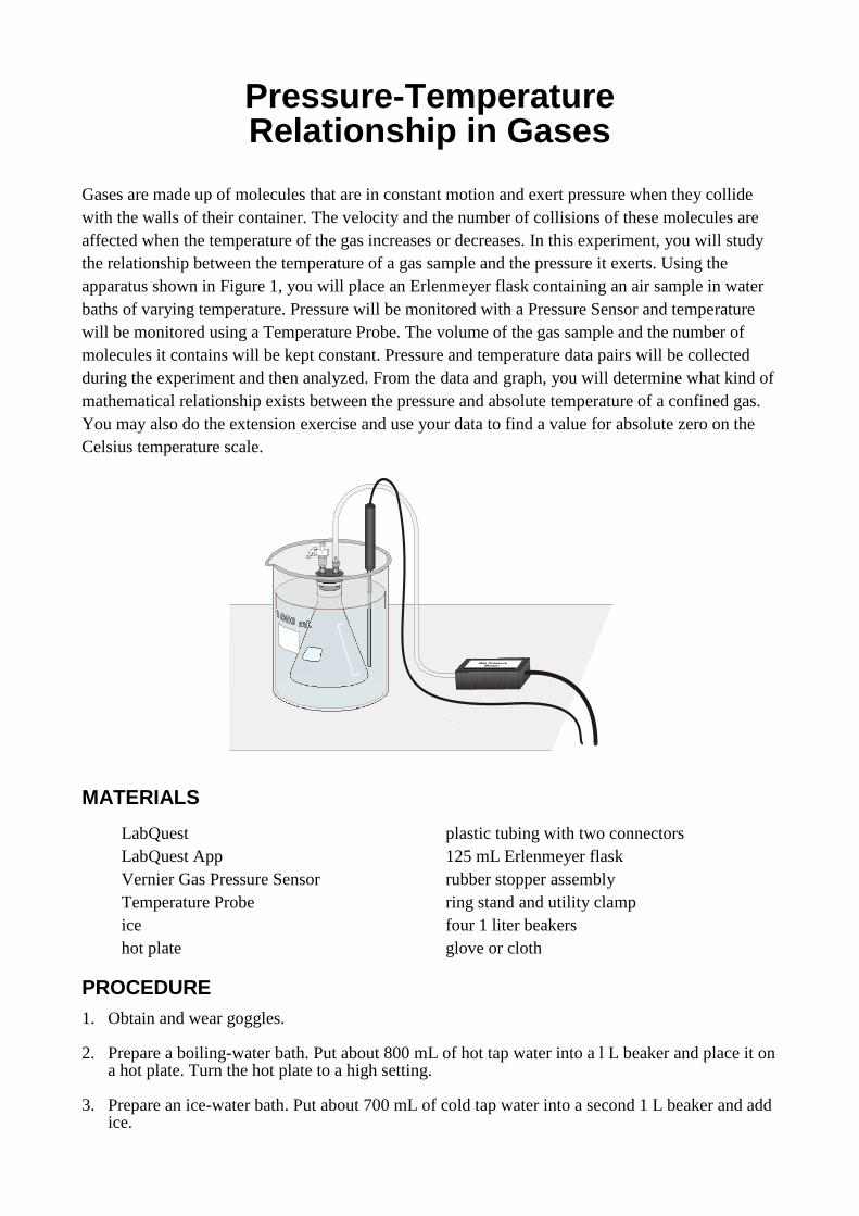
Pressure-Temperature Relationship in Gases
Gases are made up of molecules that are in constant motion and exert pressure when they collide
with the walls of their container. The velocity and the number of collisions of these molecules are
affected when the temperature of the gas increases or decreases. In this experiment, you will study
the relationship between the temperature of a gas sample and the pressure it exerts. Using the
apparatus shown in Figure 1, you will place an Erlenmeyer flask containing an air sample in water
baths of varying temperature. Pressure will be monitored with a Pressure Sensor and temperature
will be monitored using a Temperature Probe. The volume of the gas sample and the number of
molecules it contains will be kept constant. Pressure and temperature data pairs will be collected
during the experiment and then analyzed. From the data and graph, you will determine what kind of
mathematical relationship exists between the pressure and absolute temperature of a confined gas.
You may also do the extension exercise and use your data to find a value for absolute zero on the
Celsius temperature scale.
MATERIALS
LabQuest plastic tubing with two connectors
LabQuest App 125 mL Erlenmeyer flask
Vernier Gas Pressure Sensor rubber stopper assembly
Temperature Probe ring stand and utility clamp
ice four 1 liter beakers
hot plate glove or cloth
PROCEDURE
1. Obtain and wear goggles.
2. Prepare a boiling-water bath. Put about 800 mL of hot tap water into a l L beaker and place it on a hot plate. Turn the hot plate to a high setting.
3. Prepare an ice-water bath. Put about 700 mL of cold tap water into a second 1 L beaker and add ice.
4. Put about 800 mL of room-temperature water into a third 1 L beaker.
5. Put about 800 mL of hot tap water into a fourth 1 L beaker.
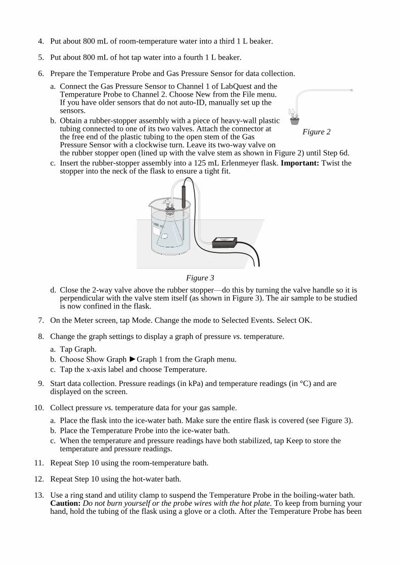
6. Prepare the Temperature Probe and Gas Pressure Sensor for data collection.
a. Connect the Gas Pressure Sensor to Channel 1 of LabQuest and the Temperature Probe to Channel 2. Choose New from the File menu. If you have older sensors that do not auto-ID, manually set up the sensors.
b. Obtain a rubber-stopper assembly with a piece of heavy-wall plastic tubing connected to one of its two valves. Attach the connector at the free end of the plastic tubing to the open stem of the Gas Pressure Sensor with a clockwise turn. Leave its two-way valve on the rubber stopper open (lined up with the valve stem as shown in Figure 2) until Step 6d.
c. Insert the rubber-stopper assembly into a 125 mL Erlenmeyer flask. Important: Twist the stopper into the neck of the flask to ensure a tight fit.
Figure 3
d. Close the 2-way valve above the rubber stopper—do this by turning the valve handle so it is perpendicular with the valve stem itself (as shown in Figure 3). The air sample to be studied is now confined in the flask.
7. On the Meter screen, tap Mode. Change the mode to Selected Events. Select OK.
8. Change the graph settings to display a graph of pressure vs. temperature.
a. Tap Graph.
b. Choose Show Graph ►Graph 1 from the Graph menu.
c. Tap the x-axis label and choose Temperature. 9. Start data collection. Pressure readings (in kPa) and temperature readings (in °C) and are
displayed on the screen.
10. Collect pressure vs. temperature data for your gas sample.
a. Place the flask into the ice-water bath. Make sure the entire flask is covered (see Figure 3).
b. Place the Temperature Probe into the ice-water bath.
c. When the temperature and pressure readings have both stabilized, tap Keep to store the temperature and pressure readings.
11. Repeat Step 10 using the room-temperature bath.
12. Repeat Step 10 using the hot-water bath.
13. Use a ring stand and utility clamp to suspend the Temperature Probe in the boiling-water bath. Caution: Do not burn yourself or the probe wires with the hot plate. To keep from burning your hand, hold the tubing of the flask using a glove or a cloth. After the Temperature Probe has been
Figure 2
in the boiling water for a few seconds, place the flask into the boiling-water bath and repeat Step 10. Stop data collection and remove the flask and the Temperature Probe.
14. Examine the data points along the displayed graph of pressure vs. temperature (°C). To examine the data pairs on the displayed graph, tap any data point. As you tap each data point, the temperature and pressure values are displayed to the right of the graph. Record the data pairs in your data table.
15. In order to determine if the relationship between pressure and temperature is direct or inverse, you must use an absolute temperature scale; that is, a temperature scale whose 0° point corresponds to absolute zero. You will use the Kelvin absolute temperature scale. Instead of manually adding 273° to each of the Celsius temperatures to obtain Kelvin values, you will create a new column for Kelvin temperature.
a. Tap the Table tab to display the data table.
b. Choose New Calculated Column from the Table menu.
c. Enter the Column Name (Kelvin Temp) and Units (K).
d. Select the equation, X+A. Use Temperature as the Column for X, and enter 273 as the value for A. Select OK to display the graph of pressure vs. Kelvin temperature.
e. Tap any data point to record the Kelvin temperature values (displayed to the right of the graph) in your data table.
16. Follow this procedure to calculate regression statistics and to plot a best-fit regression line on
your graph of pressure vs. Kelvin temperature:
a. Choose Curve Fit from the Analyze menu.
b. Select Linear as the Fit Equation. The linear-regression statistics for these two lists are displayed for the equation in the form:
y = mx + b
where x is temperature (K), y is pressure, m is a proportionality constant, and b is the y-intercept.
Select OK.
PROCESSING THE DATA
1. In order to perform this experiment, what two experimental factors were kept constant?
2. Based on the data and graph that you obtained for this experiment, express in words the relationship between gas pressure and temperature.
3. Explain this relationship using the concepts of molecular velocity and collisions of molecules.
4. Write an equation to express the relationship between pressure and temperature (K). Use the symbols P, T, and k.
5. One way to determine if a relationship is inverse or direct is to find a proportionality constant, k, from the data. If this relationship is direct, k = P/T. If it is inverse, k = P•T. Based on your answer to Question 4, choose one of these formulas and calculate k for the four ordered pairs in your data table (divide or multiply the P and T values). Show the answer in the fourth column of the Data and Calculations table. How “constant” were your values?
6. According to this experiment, what should happen to the pressure of a gas if the Kelvin temperature is doubled? Check this assumption by finding the pressure at –73°C (200 K) and at 127°C (400 K) on your graph of pressure versus temperature. How do these two pressure values compare?

RESULTS
Pressure (kPa)
Temperature (°C)
Temperature (K)
Constant, k (P / T or P•T)
EXTENSION
The data that you have collected can also be used to determine the value for absolute zero on the Celsius temperature scale. Instead of plotting pressure versus Kelvin temperature like we did above, this time you will plot Celsius temperature on the y-axis and pressure on the x-axis. Since absolute zero is the temperature at which the pressure theoretically becomes equal to zero, the temperature where the regression line (the extension of the temperature-pressure curve) intercepts the y-axis should be the Celsius temperature value for absolute zero. You can use the data you collected in this experiment to determine a value for absolute zero.
a. On the graph, change the x-axis to Pressure.
b. Change the y-axis to Temperature (°C). A graph of temperature (°C) vs. pressure is now displayed.
c. Choose Curve Fit from the Analyze menu.
d. Select Linear for the Fit Equation. The linear-regression statistics for these two lists are displayed for the equation in the form:
e. y = mx + b
f. where x is temperature (°C), y is pressure, m is a proportionality constant, and b is the y-intercept.
g. Select OK.
h. Choose Graph Options from the Graph menu. Enter 0 as the left-most value on the x-axis (Pressure). Then enter –300 as the bottom-most value on the y-axis (Temperature). Select OK.
i. Choose Interpolate from the Analyze menu. The temperature and pressure coordinate values of the regression line are displayed to the right of the graph. Tap along the regression line to a pressure value that is equal to 0 kPa. Note: You can also use the ◄ button on LabQuest to help move the cursor to 0 kPa. The temperature (in °C) at this pressure is the absolute-zero value for your data.
j. (optional) Print a graph of temperature vs. pressure, with a regression line and extrapolated temperature value displayed.
Pressure
absolutezero
A Good Cold Pack
Cold packs are used to treat sprained ankles and similar injuries. A cold pack is typically made of a
thin plastic inner bag containing water. That bag, in turn, is surrounded by a heavier plastic bag
containing a solid substance. When the pack is twisted, the inner bag breaks and releases the water.
As the solid substance dissolves in the water, energy is absorbed and the resulting mixture gets
colder.
In this experiment, you will first determine temperature changes as several different solid
substances dissolve in water. You will then develop and test a plan for making the best cold pack
using 3.0 grams of one of the substances and the best amount of water.
MATERIALS
LabQuest 10 mL graduated cylinder LabQuest App water Temperature Probe ammonium chloride, NH4Cl
balance citric acid, H3C6H5O7 weighing paper potassium chloride, KCl 50 mL beaker sodium bicarbonate, NaHCO3 250 mL beaker sodium carbonate, Na2CO3
PROCEDURE
1. Obtain and wear goggles.
2. Connect the Temperature Probe to LabQuest and choose New from the File menu. If you
have an older sensor that does not auto-ID, manually set up the sensor.
3. On the Sensor screen, tap Rate. Change the data-collection rate to 0.5 samples/second and
the data-collection length to 300 seconds (5 minutes).
4. Measure out 3.0 g of each of the test substances. Use and label a new piece of weighing
paper for each substance.
5. Use a 10 mL graduated cylinder to measure out 10 mL of room-temperature water into a
clean 50 mL beaker.
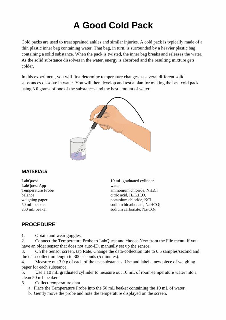
6. Collect temperature data.
a. Place the Temperature Probe into the 50 mL beaker containing the 10 mL of water.
b. Gently move the probe and note the temperature displayed on the screen.
c. When the temperature stops changing, start data collection.
d. Monitor the temperature for 15 seconds to establish the initial temperature of the water.
e. Carefully add the solid ammonium chloride, NH4Cl, to the water. Stir gently with the
Temperature Probe.
f. When the temperature stops changing, stop data collection.
7. Record the minimum and maximum temperatures.
a. To examine the data pairs on the displayed graph, tap any data point. As you tap each data
point, the temperature value of each data point is displayed to the right of the graph.
b. Record your minimum and maximum temperatures in your data table.
c. Tap Meter.
8. Repeat Steps 5–7 for each of the remaining substances. Clean the probe after each
run and place it into a 250 mL beaker containing room-temperature water to bring the probe back to
room temperature.
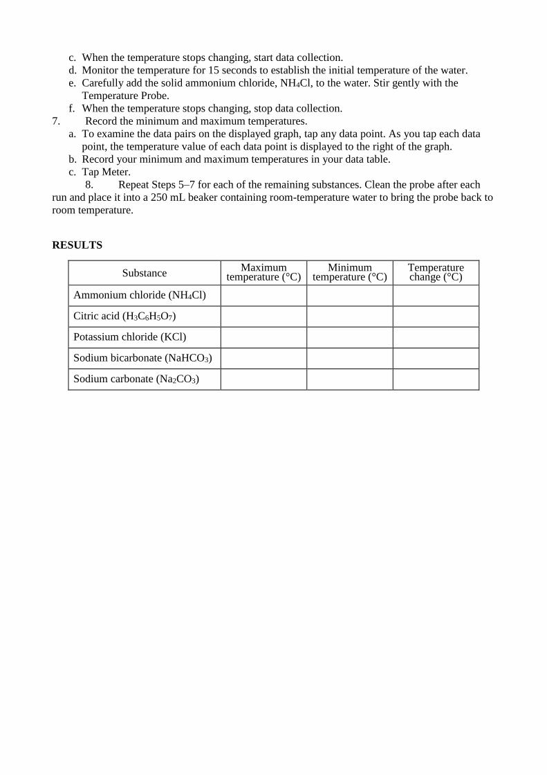
RESULTS
Substance Maximum
temperature (°C) Minimum
temperature (°C) Temperature change (°C)
Ammonium chloride (NH4Cl)
Citric acid (H3C6H5O7)
Potassium chloride (KCl)
Sodium bicarbonate (NaHCO3)
Sodium carbonate (Na2CO3)
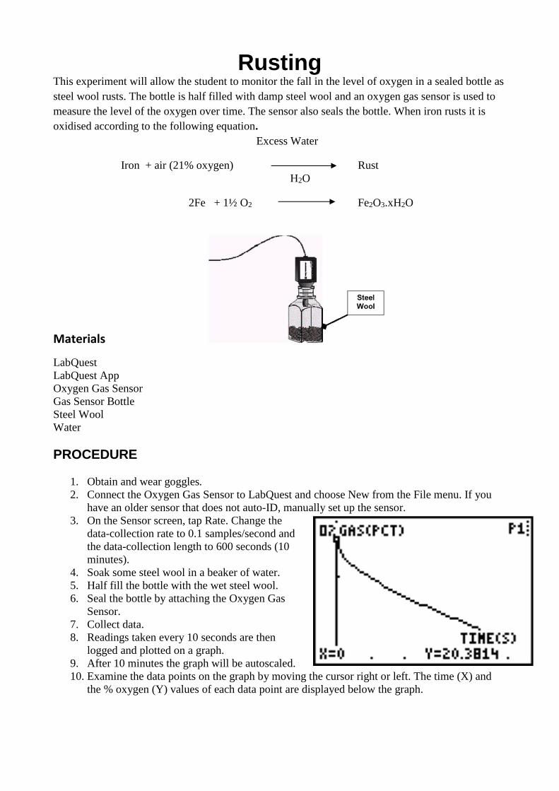
Rusting This experiment will allow the student to monitor the fall in the level of oxygen in a sealed bottle as
steel wool rusts. The bottle is half filled with damp steel wool and an oxygen gas sensor is used to
measure the level of the oxygen over time. The sensor also seals the bottle. When iron rusts it is
oxidised according to the following equation. Excess Water
Iron + air (21% oxygen) Rust
H2O
2Fe + 1½ O2 Fe2O3.xH2O
Materials
LabQuest
LabQuest App
Oxygen Gas Sensor
Gas Sensor Bottle
Steel Wool
Water
PROCEDURE
1. Obtain and wear goggles.
2. Connect the Oxygen Gas Sensor to LabQuest and choose New from the File menu. If you
have an older sensor that does not auto-ID, manually set up the sensor.
3. On the Sensor screen, tap Rate. Change the
data-collection rate to 0.1 samples/second and
the data-collection length to 600 seconds (10
minutes).
4. Soak some steel wool in a beaker of water.
5. Half fill the bottle with the wet steel wool.
6. Seal the bottle by attaching the Oxygen Gas
Sensor.
7. Collect data.
8. Readings taken every 10 seconds are then
logged and plotted on a graph.
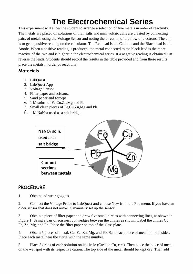
9. After 10 minutes the graph will be autoscaled.
10. Examine the data points on the graph by moving the cursor right or left. The time (X) and
the % oxygen (Y) values of each data point are displayed below the graph.
The Electrochemical Series This experiment will allow the student to arrange a selection of five metals in order of reactivity.
The metals are placed on solutions of their salts and mini voltaic cells are created by connecting
pairs of metals using the Voltage Sensor and noting the direction of the flow of electrons. The aim
is to get a positive reading on the calculator. The Red lead is the Cathode and the Black lead is the
Anode. When a positive reading is produced, the metal connected to the black lead is the more
reactive of the two and is higher in the electrochemical series. If a negative reading is obtained just
reverse the leads. Students should record the results in the table provided and from these results
place the metals in order of reactivity.
Materials
1. LabQuest
2. LabQuest App
3. Voltage Sensor.
4. Filter paper and scissors.
5. Sand paper and forceps
6. 1 M solns. of Fe,Cu,Zn,Mg and Pb
7. Small clean pieces of Fe,Cu,Zn,Mg and Pb
8. 1 M NaNo3 used as a salt bridge
PROCEDURE
1. Obtain and wear goggles.
2. Connect the Voltage Probe to LabQuest and choose New from the File menu. If you have an
older sensor that does not auto-ID, manually set up the sensor.
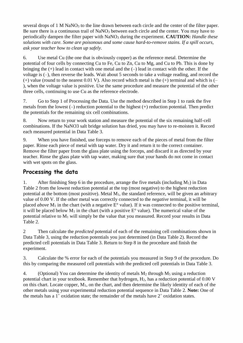
3. Obtain a piece of filter paper and draw five small circles with connecting lines, as shown in
Figure 1. Using a pair of scissors, cut wedges between the circles as shown. Label the circles Cu,
Fe, Zn, Mg, and Pb. Place the filter paper on top of the glass plate.
4. Obtain 5 pieces of metal, Cu, Fe, Zn, Mg, and Pb. Sand each piece of metal on both sides.
Place each metal near the circle with the same number.
5. Place 3 drops of each solution on its circle (Cu2+ on Cu, etc.). Then place the piece of metal
on the wet spot with its respective cation. The top side of the metal should be kept dry. Then add
NaNO3 soln.
used as a
salt bridge
Cut out
sections
between metals
several drops of 1 M NaNO3 to the line drawn between each circle and the center of the filter paper.
Be sure there is a continuous trail of NaNO3 between each circle and the center. You may have to
periodically dampen the filter paper with NaNO3 during the experiment. CAUTION: Handle these
solutions with care. Some are poisonous and some cause hard-to-remove stains. If a spill occurs,
ask your teacher how to clean up safely.
6. Use metal Cu (the one that is obviously copper) as the reference metal. Determine the
potential of four cells by connecting Cu to Fe, Cu to Zn, Cu to Mg, and Cu to Pb. This is done by
bringing the (+) lead in contact with one metal and the (–) lead in contact with the other. If the
voltage is (–), then reverse the leads. Wait about 5 seconds to take a voltage reading, and record the
(+) value (round to the nearest 0.01 V). Also record which metal is the (+) terminal and which is (–
), when the voltage value is positive. Use the same procedure and measure the potential of the other
three cells, continuing to use Cu as the reference electrode.
7. Go to Step 1 of Processing the Data. Use the method described in Step 1 to rank the five
metals from the lowest (–) reduction potential to the highest (+) reduction potential. Then predict
the potentials for the remaining six cell combinations.
8. Now return to your work station and measure the potential of the six remaining half-cell
combinations. If the NaNO3 salt bridge solution has dried, you may have to re-moisten it. Record
each measured potential in Data Table 3.
9. When you have finished, use forceps to remove each of the pieces of metal from the filter
paper. Rinse each piece of metal with tap water. Dry it and return it to the correct container.
Remove the filter paper from the glass plate using the forceps, and discard it as directed by your
teacher. Rinse the glass plate with tap water, making sure that your hands do not come in contact
with wet spots on the glass.
Processing the data
1. After finishing Step 6 in the procedure, arrange the five metals (including M1) in Data
Table 2 from the lowest reduction potential at the top (most negative) to the highest reduction
potential at the bottom (most positive). Metal M1, the standard reference, will be given an arbitrary
value of 0.00 V. If the other metal was correctly connected to the negative terminal, it will be
placed above M1 in the chart (with a negative E° value). If it was connected to the positive terminal,
it will be placed below M1 in the chart (with a positive E° value). The numerical value of the
potential relative to M1 will simply be the value that you measured. Record your results in Data
Table 2.
2 Then calculate the predicted potential of each of the remaining cell combinations shown in
Data Table 3, using the reduction potentials you just determined (in Data Table 2). Record the
predicted cell potentials in Data Table 3. Return to Step 8 in the procedure and finish the
experiment.
3. Calculate the % error for each of the potentials you measured in Step 9 of the procedure. Do
this by comparing the measured cell potentials with the predicted cell potentials in Data Table 3.
4. (Optional) You can determine the identity of metals M2 through M5 using a reduction
potential chart in your textbook. Remember that hydrogen, H2, has a reduction potential of 0.00 V
on this chart. Locate copper, M1, on the chart, and then determine the likely identity of each of the
other metals using your experimental reduction potential sequence in Data Table 2. Note: One of
the metals has a 1+ oxidation state; the remainder of the metals have 2+ oxidation states.
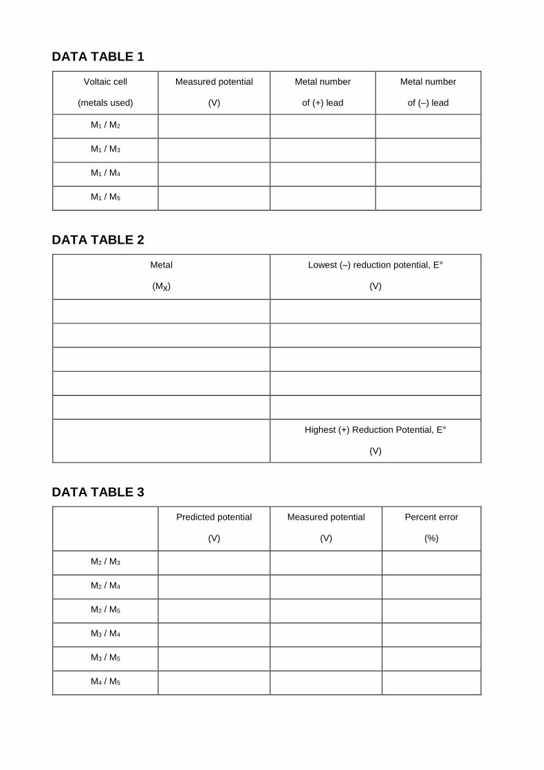
DATA TABLE 1
Voltaic cell
(metals used)
Measured potential
(V)
Metal number
of (+) lead
Metal number
of (–) lead
M1 / M2
M1 / M3
M1 / M4
M1 / M5
DATA TABLE 2
Metal
(Mx)
Lowest (–) reduction potential, E°
(V)
Highest (+) Reduction Potential, E°
(V)
DATA TABLE 3
Predicted potential
(V)
Measured potential
(V)
Percent error
(%)
M2 / M3
M2 / M4
M2 / M5
M3 / M4
M3 / M5
M4 / M5
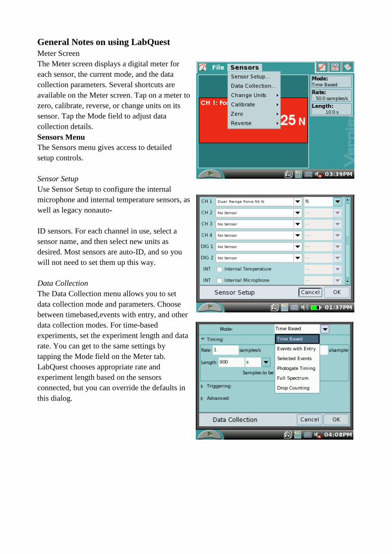
General Notes on using LabQuest
Meter Screen
The Meter screen displays a digital meter for
each sensor, the current mode, and the data
collection parameters. Several shortcuts are
available on the Meter screen. Tap on a meter to
zero, calibrate, reverse, or change units on its
sensor. Tap the Mode field to adjust data
collection details.
Sensors Menu
The Sensors menu gives access to detailed
setup controls.
Sensor Setup
Use Sensor Setup to configure the internal
microphone and internal temperature sensors, as
well as legacy nonauto-
ID sensors. For each channel in use, select a
sensor name, and then select new units as
desired. Most sensors are auto-ID, and so you
will not need to set them up this way.
Data Collection
The Data Collection menu allows you to set
data collection mode and parameters. Choose
between timebased,events with entry, and other
data collection modes. For time-based
experiments, set the experiment length and data
rate. You can get to the same settings by
tapping the Mode field on the Meter tab.
LabQuest chooses appropriate rate and
experiment length based on the sensors
connected, but you can override the defaults in
this dialog.