Embed Size (px)
Citation preview
NewsThe Newsletter of the R Project Volume 1/2, June 2001
Editorialby Kurt Hornik and Friedrich Leisch
Welcome to the second issue of R News, the newslet-ter of the R project for statistical computing. First wewould like to thank for all the positive feedback wegot on the first volume, which encourages us verymuch to continue with this online magazine.
A lot has happened since the first volume ap-peared last January, especially the workshop “DSC2001” comes to mind. More on this remarkable eventcan be found in the new regular column “RecentEvents”. During DSC 2001 the R Core Team washappy to announce Stefano Iacus (who created theMacintosh port of R) as a new member of R Core:Welcome aboard, Stefano!
We have started collecting an annotated R bibli-ography, see http://www.R-project.org/doc/bib/R-publications.html. It will list books, journal ar-ticles, . . . that may be useful to the R user community(and are related to R or S). If you are aware of anypublications that should be included in the bibliog-raphy, please send email to [email protected].
To make citation easier we have registered anISSN number for this newsletter: ISSN 1609-3631.Please use this number together with the homepage of the newsletter (http://cran.R-project.org/doc/Rnews/) when citing articles from R News.
We are now planning to have 4 issues of R News
per year, scheduled for March/April, June/July,September/October and December/January, respec-tively. This should fit nicely into the calendar of the(Austrian) academic year and allow the editors to domost of the production work for at least 3 issues dur-ing semester breaks or holidays (remember that cur-rently, all of the R project including this newsletter isvolunteer work). Hence, the next issue is due after(northern hemisphere) summer: all contributions arewelcome!
R 1.3.0 has just been released, and its new featuresare described in “Changes in R”. Alongside, severaladd-on packages from CRAN have been categorizedas recommended and will be available in all binary dis-tributions of R in the future (“Changes on CRAN”has more details). R News will provide introductoryarticles on each recommended package, starting inthis issue with “mgcv: GAMs and Generalized RidgeRegression for R”.
Kurt HornikWirtschaftsuniversität Wien, AustriaTechnische Universität Wien, [email protected]
Friedrich LeischTechnische Universität Wien, [email protected]
Contents of this issue:
Editorial . . . . . . . . . . . . . . . . . . . . . . 1Changes in R . . . . . . . . . . . . . . . . . . . . 1Changes on CRAN . . . . . . . . . . . . . . . . 5Date-Time Classes . . . . . . . . . . . . . . . . . 8Installing R under Windows . . . . . . . . . . . 11Spatial Statistics in R . . . . . . . . . . . . . . . 14
geoR: A Package for Geostatistical Analysis . . 15Simulation and Analysis of Random Fields . . 18mgcv: GAMs and Generalized Ridge Regres-
sion for R . . . . . . . . . . . . . . . . . . . . 20What’s the Point of ‘tensor’? . . . . . . . . . . . 26On Multivariate t and Gauß Probabilities in R . 27Programmer’s Niche . . . . . . . . . . . . . . . 29Recent Events . . . . . . . . . . . . . . . . . . . 32
Vol. 1/2, June 2001 2
Changes in Rby the R Core Team
New features in version 1.3.0
• Changes to connections:
– New function url() to read from URLs.file() will also accept URL specifica-tions, as will all the functions which useit.
– File connections can now be opened forboth reading and writing.
– Anonymous file connections (via file())are now supported.
– New function gzfile() to read from /write to compressed files.
– New function fifo() for connections to /from fifos (on Unix).
– Text input from file, pipe, fifo, gzfile andurl connections can be read with a user-specified encoding.
– New functions readChar() to read char-acter strings with known lengths and noterminators, and writeChar() to writeuser-specified lengths from strings.
– sink() now has a stack of output connec-tions, following S4.
– sink() can also be applied to the messagestream, to capture error messages to a con-nection. Use carefully!
– seek() has a new ‘origin’ argument.– New function truncate() to truncate a
connection open for writing at the currentposition.
– New function socketConnection() forsocket connections.
– The ‘blocking’ argument for file, fifo andsocket connections is now operational.
• Changes to date/time classes and functions:
– Date/time objects now all inherit fromclass "POSIXt".
– New function difftime() and corre-sponding class for date/time differences,and a round() method.
– Subtraction and logical comparison of ob-jects from different date/time classes isnow supported. NB: the format for thedifference of two objects of the samedate/time class has changed, but onlyfor objects generated by this version, notthose generated by earlier ones.
– Methods for cut(), seq(), round() andtrunc() for date/time classes.
– Convenience generic functions julian(),weekdays(), months(), and quarters()with methods for "POSIXt" objects.
• Coercion from real to integer now gives NA forout-of-range values, rather than the most ex-treme integer of the same sign.
• The Ansari-Bradley, Bartlett, Fligner-Killeen,Friedman, Kruskal-Wallis, Mood, Quade, t,and Wilcoxon tests as well as var.test() inpackage ctest now have formula interfaces.
• The matrix multiplication functions %*% andcrossprod() now use a level-3 BLAS routinedgemm. When R is linked with the ATLAS orother enhanced BLAS libraries this can be sub-stantially faster than the previous code.
• New functions La.eigen() and La.svd() foreigenvector and singular value decomposi-tions, based on LAPACK. These are preferredto eigen() and svd() for new projects andcan make use of enhanced BLAS routinessuch as ATLAS. They are used in cancor(),cmdscale(), factanal() and princomp() andthis may lead to sign reversals in some of theoutput of those functions.
• Provided the FORTRAN compiler can handleCOMPLEX*16, the following routines now han-dle complex arguments, based on LAPACKcode: qr(), qr.coef(), qr.solve(), qr.qy(),qr.qty(), solve.default(), svd(), La.svd().
• aperm() uses strides in the internal C code andso is substantially faster (by Jonathan Rougier).
• The four bessel[IJKY](x,nu) functions arenow defined for nu < 0.
• [dpqr]nbinom() also accept an alternativeparametrization via the mean and the disper-sion parameter (thanks to Ben Bolker).
• New generalised “birthday paradox” functions[pq]birthday().
• boxplot() and bxp() have a new argument‘at’.
• New function capabilities() to report op-tional capabilities such as jpeg, png, tcltk, gzfileand url support.
• New function checkFF() for checking foreignfunction calls.
R News ISSN 1609-3631
Vol. 1/2, June 2001 3
• New function col2rgb() for color conversionof names, hex, or integer.
• coplot() has a new argument ‘bar.bg’ (color ofconditioning bars), gives nicer plots when theconditioners are factors, and allows factors forx and y (treated almost as if unclass()ed) us-ing new argument ‘axlabels’. [Original ideas byThomas Baummann]
• ‘hessian’ argument added to deriv() and itsmethods. A new function deriv3() providesidentical capabilities to deriv() except that‘hessian’ is TRUE by default. deriv(*, *, func= TRUE) for convenience.
• New dev.interactive() function, useful forsetting defaults for par(ask=*) in multifigureplots.
• dist() in package mva can now handle miss-ing values, and zeroes in the Canberra distance.
• The default method for download.file()(and functions which use it such asupdate.packages()) is now "internal", anduses code compiled into R.
• eigen() tests for symmetry with a numericaltolerance.
• New function formatDL() for formatting de-scription lists.
• New argument ‘nsmall’ to format.default(),for S-PLUS compatibility (and used in variouspackages).
• ?/help() now advertises help.search() if itfails to find a topic.
• image() is now a generic function.
• New function integrate() with S-compatiblecall.
• New function is.unsorted() the C version ofwhich also speeds up .Internal(sort()) forsorted input.
• is.loaded() accepts an argument ‘PACKAGE’to search within a specific DLL/shared library.
• Exact p-values are available for the two-sidedtwo-sample Kolmogorov-Smirnov test.
• lm() now passes ‘. . . ’ to the low level functionsfor regression fitting.
• Generic functions logLik() and AIC() movedfrom packages nls and nlme to base, as well astheir lm methods.
• New components in .Machine give the sizes oflong, long long and long double C types (or0 if they do not exist).
• merge.data.frame() has new arguments,‘all[.xy]’ and ‘suffixes’, for S compatibility.
• model.frame() now calls na.action with theterms attribute set on the data frame (neededto distiguish the response, for example).
• New generic functions naprint(), naresid(),and napredict() (formerly in packages MASSand survival5, also used in package rpart).Also na.exclude(), a variant on na.omit()that is handled differently by naresid() andnapredict().
The default, lm and glm methods for fitted(),residuals(), predict() and weights() makeuse of these.
• New function oneway.test() in package ctestfor testing for equal means in a one-way layout,assuming normality but not necessarily equalvariances.
• options(error) accepts a function, as an alter-native to an expression. (The Blue Book onlyallows a function; current S-PLUS a function oran expression.)
• outer() has a speed-up in the default case of amatrix outer product (by Jonathan Rougier).
• package.skeleton() helps with creating newpackages.
• New pdf() graphics driver.
• persp() is now a generic function.
• plot.acf() makes better use of white spacefor ‘nser > 2’, has new optional arguments anduses a much better layout when more than onepage of plots is produced.
• plot.mts() has a new argument ‘panel’ pro-viding the same functionality as in coplot().
• postscript() allows user-specified encoding,with encoding files supplied for Windows,Mac, Unicode and various others, and with anappropriate platform-specific default.
• print.htest() can now handle test names thatare longer than one line.
• prompt() improved for data sets, particularlynon-dataframes.
• qqnorm() is now a generic function.
• read.fwf() has a new argument ‘n’ for speci-fying the number of records (lines) read in.
• read.table() now uses a single pass throughthe dataset.
R News ISSN 1609-3631
Vol. 1/2, June 2001 4
• rep() now handles lists (as generic vectors).
• scan() has a new argument ‘multi.line’ for Scompatibility, but the default remains the op-posite of S (records can cross line boundariesby default).
• sort(x) now produces an error when x is notatomic instead of just returning x.
• split() now allows splitting on a list of fac-tors in which case their interaction defines thegrouping.
• stl() has more optional arguments for finetuning, a summary() and an improved plot()method.
• New function strwrap() for formatting char-acter strings into paragraphs.
• New replacement functions substr<-() andsubstring<-().
• Dataset swiss now has row names.
• Arguments ‘pkg’ and ‘lib’ of system.file()have been renamed to ‘package’ and ‘lib.loc’,respectively, to be consistent with related func-tions. The old names are deprecated. Argu-ment ‘package’ must now specify a single pack-age.
• The Wilcoxon and Ansari-Bradley tests now re-turn point estimators of the location or scale pa-rameter of interest along with confidence inter-vals for these.
• New function write.dcf() for writing datain Debian Control File format. parse.dcf()has been replaced by (much faster) internalread.dcf().
• Contingency tables created by xtabs() ortable() now have a summary() method.
• Functions httpclient(), read.table.url(),scan.url() and source.url() are now dep-recated, and hence ‘method="socket"’ indownload.file() is. Use url connections in-stead: in particular URLs can be specified forread.table(), scan() and source().
• Formerly deprecated function getenv() is nowdefunct.
• Support for package-specific demo scripts (Rcode). demo() now has new arguments to spec-ify the location of demos and to allow for run-ning base demos as part of ‘make check’.
• If not explicitly given a library tree to install toor remove from, respectively, R CMD INSTALLand R CMD REMOVE now operate on the first di-rectory given in R_LIBS if this is set and non-null, and the default library otherwise.
• R CMD INSTALL and package.description()fix some common problems of ‘DESCRIPTION’files (blank lines, . . . ).
• The INSTALL command for package installationallows a ‘--save’ option. Using it causes a bi-nary image of the package contents to be cre-ated at install time and loaded when the pack-age is attached. This saves time, but also uses amore standard way of source-ing the package.Packages that do more than just assign objectdefinitions may need to install with ‘--save’.Putting a file ‘install.R’ in the package directorymakes ‘--save’ the default behavior. If thatfile is not empty, its contents should be R com-mands executed at the end of creating the im-age.
There is also a new command line option‘--configure-vals’ for passing variables tothe configure script of a package.
• R CMD check now also checks the keyword en-tries against the list of standard keywords,for code/documentation mismatches (this canbe turned off by the command line option‘--no-codoc’), and for sufficient file permis-sions (Unix only). There is a new check for thecorrect usage of library.dynam().
It also has a new command line option‘--use-gct’ to use ‘gctorture(TRUE)’ whenrunning R code.
• R CMD Rd2dvi has better support for produc-ing reference manuals for packages and pack-age bundles.
• configure now tests for the versions of jpeg(≥ 6b), libpng (≥ 1.0.5) and zlib (≥ 1.1.3). Itno longer checks for the CXML/DXML BLASlibraries on Alphas.
• Perl scripts now use Cwd::cwd() in place ofCwd::getcwd(), as cwd() can be much faster.
• ‘R::Dcf.pm’ can now also handle files with morethan one record and checks (a little bit) for con-tinuation lines without leading whitespace.
• New manual ‘R Installation and Administra-tion’ with fuller details on the installation pro-cess: file ‘INSTALL’ is now a brief introductionreferencing that manual.
• New keyword ‘internal’ which can be used tohide objects that are not part of the API fromindices like the alphabetical lists in the HTMLhelp system.
R News ISSN 1609-3631
Vol. 1/2, June 2001 5
• Under Unix, shlib modules for add-on pack-ages are now linked against R as a shared li-brary (‘libR’) if this exists. (This allows forimproved embedding of R into other applica-tions.)
• New mechanism for explicitly registering na-tive routines in a DLL/shared library ac-cessible via .C(), .Call(), .Fortran() and.External(). This is potentially more ro-bust than the existing dynamic lookup, since itchecks the number of arguments, type of theroutine.
• New mechanism allowing registration of Croutines for converting R objects to C pointersin .C() calls. Useful for references to data inother languages and libraries (e.g. C and hdf5).
• The internal ftp/http access code maintains theevent loop, so you can download whilst run-ning tcltk or Rggobi, say. It can be hooked intopackage XML too.
New features in version 1.2.3
• Support for configuration and building theUnix version of R under Mac OS X. (The ‘clas-sic’ Macintosh port is ‘Carbonized’ and alsoruns under that OS.)
• dotchart() and stripchart() becomethe preferred names for dotplot() andstripplot(), respectively. The old names arenow deprecated.
• Functions in package ctest now consistentlyuse +/-Inf rather than NA for one-sided confi-dence intervals.
New features in version 1.2.2
• The Macintosh port becomes a full member ofthe R family and its sources are incorporated asfrom this release. See ‘src/macintosh/INSTALL’for how that port is built.
• The API header files and export files ‘R.exp’ arereleased under LGPL rather than GPL to allowdynamically loaded code to be distributed un-der licences other than GPL.
• postscript() and xfig() devices now makeuse of genuine Adobe afm files, and warn ifcharacters are used in string width or heightcalculations that are not in the afm files.
• Configure now uses a much expanded searchlist for finding a FORTRAN 77 compiler, and nolonger disallows wrapper scripts for this com-piler.
• New Rd markup \method{GENERIC}{CLASS}for indicating the usage of methods.
• print.ftable() and write.ftable() nowhave a ‘digits’ argument.
• undoc() has a new ‘lib.loc’ argument, and itsfirst argument is now called ‘package’.
Changes on CRANby Kurt Hornik and Friedrich Leisch
CRAN packages
The following extension packages from ‘src/contrib’were added since the last newsletter.
AnalyzeIO Functions for I/O of ANALYZE imageformat files. By Jonathan L Marchini.
CoCoAn Two functions to compute correspondenceanalysis and constrained correspondence anal-ysis and to make the associated graphical rep-resentation. By Stephane Dray.
GLMMGibbs Generalised Linear Mixed Models arean extension of Generalised Linear Modelsto include non-independent responses. Thispackage allows them to be fitted by including
functions for declaring factors to be random ef-fects, for fitting models and generic functionsfor examining the fits. By Jonathan Myles andDavid Clayton.
GeneSOM Clustering Genes using Self-OrganizingMap. By Jun Yan.
Oarray Generalise the starting point of the array in-dex, e.g. to allow x[0, 0, 0] to be the first el-ement of x. By Jonathan Rougier.
PTAk A multiway method to decompose a tensor(array) of any order, as a generalisation of SVDalso supporting non-identity metrics and pe-nalisations. 2-way SVD with these extensionsis also available. The package includes alsosome other multiway methods: PCAn (Tucker-n) and PARAFAC/CANDECOMP with theseextensions. By Didier Leibovici.
R News ISSN 1609-3631
Vol. 1/2, June 2001 6
RArcInfo This package uses the functions writtenby Daniel Morissette ([email protected]) toread geographical information in Arc/Info V7.x format to import the coverages into R vari-ables. By Virgilio Gómez-Rubio.
RMySQL DataBase Interface and MySQL driver forR. By David A. James and Saikat DebRoy.
RandomFields Simulating and analysing randomfields using various methods. By MartinSchlather.
SuppDists Ten distributions supplementing thosebuilt into R. Inverse Gauss, Kruskal-Wallis,Kendall’s Tau, Friedman’s chi squared, Spear-man’s rho, maximum F ratio, the Pearsonproduct moment correlation coefficiant, John-son distributions, normal scores and general-ized hypergeometric distributions. In addi-tion two random number generators of GeorgeMarsaglia are included. By Bob Wheeler.
adapt Adaptive quadrature in up to 20 dimensions.By Thomas Lumley.
blighty Function for drawing the coastline of theUnited Kingdom. By David Lucy.
bqtl QTL mapping toolkit for inbred crosses and re-combinant inbred lines. Includes maximumlikelihood and Bayesian tools. By Charles C.Berry.
cramer Provides R routine for the multivariate non-parametric Cramer-Test. By Carsten Franz.
event.chart The function event.chart creates anevent chart on the current graphics device. Soriginal by J. Lee, K. Hess and J. Dubin. R portby Laura Pontiggia.
geoR Functions to perform geostatistical analysis in-cluding model-based methods. By Paulo J.Ribeiro Jr and Peter J. Diggle.
gregmisc Misc Functions written/maintained byGregory R. Warnes. By Gregory R. Warnes. In-cludes code provided by William Venables andBen Bolker.
lgtdl A very simple implementation of a class forlongitudinal data. See the corresponding paperin the DSC-2001 proceedings. By Robert Gen-tleman.
lokern Kernel regression smoothing with adaptivelocal or global plug-in bandwidth selection., ByEva Herrmann (FORTRAN 77 & S original);Packaged for R by Martin Maechler.
lpridge lpridge and lpepa provide local poly-nomial regression algorithms including localbandwidth use. By Burkhardt Seifert (S origi-nal); packaged for R by Martin Maechler.
maxstat Maximally selected rank and Gauss statis-tics with several p-value approximations. ByTorsten Hothorn and Berthold Lausen.
meanscore The Mean Score method for missing andauxiliary covariate data is described in the pa-per by Reilly & Pepe in Biometrika 1995. Thislikelihood-based method allows an analysis us-ing all available cases and hence will give moreefficient estimates. The method is applicable tocohort or case-control designs. By Marie ReillyPhD and Agus Salim.
netCDF Read data from netCDF files. By ThomasLumley, based on code by Steve Oncley andGordon Maclean.
nlrq Nonlinear quantile regression routines. ByRoger Koenker and Philippe Grosjean.
odesolve This package provides an interface for theODE solver lsoda. ODEs are expressed as Rfunctions. By R. Woodrow Setzer with fixupsby Martin Maechler.
panel Functions and datasets for fitting models toPanel data. By Robert Gentleman.
permax Functions intended to facilitate certain ba-sic analyses of DNA array data, especially withregard to comparing expression levels betweentwo types of tissue. By Robert J. Gray.
pinktoe Converts S tree objects into HTML/perlfiles. These web files can be used to interac-tively traverse the tree on a web browser. Thisweb based approach to traversing trees is espe-cially useful for large trees or for trees wherethe text for each variable is verbose. By GuyNason.
sma The package contains some simple functions forexploratory microarray analysis. By SandrineDudoit, Yee Hwa (Jean) Yang and BenjaminMilo Bolstad, with contributions from NatalieThorne, Ingrid Lönnstedt, and Jessica Mar.
sna A range of tools for social network analysis, in-cluding node and graph-level indices, struc-tural distance and covariance methods, struc-tural equivalence detection, p∗ modeling, andnetwork visualization. By Carter T. Butts.
strucchange Testing on structural change in lin-ear regression relationships. It featurestests/methods from the generalized fluctua-tion test framework as well as from the F test(Chow test) framework. This includes meth-ods to fit, plot and test fluctuation processes
R News ISSN 1609-3631
Vol. 1/2, June 2001 7
(e.g., CUSUM, MOSUM, recursive/moving es-timates) and F statistics, respectively. Further-more it is possible to monitor incoming dataonline. By Achim Zeileis, Friedrich Leisch,Bruce Hansen, Kurt Hornik, Christian Kleiber,and Andrea Peters.
twostage Functions for optimal design of two-stage-studies using the Mean Score method. ByMarie Reilly PhD and Agus Salim.
CRAN mirrors the R packages from the Omega-hat project in directory ‘src/contrib/Omegahat’. Thefollowing are recent additions:
OOP OOP style classes and methods for R and S-Plus. Object references and class-based methoddefinition are supported in the style of lan-guages such as Java and C++. By John Cham-bers and Duncan Temple Lang.
RGnumeric A plugin for the Gnumeric spreadsheetthat allows R functions to be called from cellswithin the sheet, automatic recalculation, etc.By Duncan Temple Lang.
RJavaDevice A graphics device for R that uses Javacomponents and graphics APIs. By DuncanTemple Lang.
RSPython Allows Python programs to invoke Sfunctions, methods, etc. and S code to callPython functionality. This uses a general for-eign reference mechanism to avoid copyingand translating object contents and definitions.By Duncan Temple Lang.
SLanguage Functions and C support utilities to sup-port S language programming that can work inboth R and S-Plus. By John Chambers.
SNetscape R running within Netscape for dynamic,statistical documents, with an interface to andfrom JavaScript and other plugins. By DuncanTemple Lang.
SXalan Process XML documents using XSL func-tions implemented in R and dynamically sub-stituting output from R. By Duncan TempleLang.
Slcc Parses C source code, allowing one to analyzeand automatically generate interfaces from Sto that code, including the table of S-accessiblenative symbols, parameter count and type in-formation, S constructors from C objects, callgraphs, etc. By Duncan Temple Lang.
Recommended packages
The number of packages on CRAN has grown over100 recently, ranging from big toolboxes with a long
history in the S community (like nlme or survival)to more specialized smaller packages (like the geo-statistical packages described later in this volume ofR News). To make orientation for users, package de-velopers and providers of binary distributions easierwe have decided to start categorizing the contributedpackages on CRAN.
Up to now there have been 2 categories of pack-ages: Packages with priority base that come directlywith the sources of R (like ctest, mva or ts) and all therest. As a start for finer granularity we have intro-duced the new priority recommended for the follow-ing packages: KernSmooth, VR (bundle of MASS,class, nnet, spatial), boot, cluster, foreign, mgcv,nlme, rpart and survival.
Criteria for priority recommended are:
• Actively maintained and good quality codethat can be installed on all (major) platforms.
• Useful for a wider audience in the sense thatusers “would expect this functionality” from ageneral purpose statistics environment like R.
• Depend only on packages with priority base orrecommended.
All binary distributions of R (that are availablefrom CRAN) will at least include the recommendedpackages in the future. Hence, if you write a packagethat depends on a recommended package it shouldbe no problem for users of your package to meet thisrequirement (as most likely the recommended pack-ages are installed anyway). In some sense the “min-imum typical R installation” is the base system plusthe recommended packages.
A final note: This is of course no judgement atall about the quality of all the other packages onCRAN. It is just the (subjective) opinion of the R CoreTeam what a minimum R installation should include.The criterion we used most for compiling the list ofrecommended packages was whether we thought apackage was useful for a wide audience.
MacOS and MacOS X
Starting from release 1.3.0 of R two different versionsof R for Macintosh are available at CRAN in two sep-arate folders: ‘bin/macos’ and ‘bin/macosx’.
The ‘bin/macos’ folder contains a version in-tended to run on Macintosh machines running Sys-tem 8.6 to 9.1 and which will run on MacOS X as acarbon application, thus natively. The folder has thesame structure as it was for release 1.2.x. Now thebase distribution is available as two versions:
‘rm130.sit’ contains the base R distribution withoutthe recommended packages;
‘rm130 FULL.sit’ contains the base distributionalong with all recommended packages.
R News ISSN 1609-3631
Vol. 1/2, June 2001 8
It is possible at a later time to download the archive‘recommended.sit’ that contains the additional rec-ommended packages not included in the base-onlypackage. As usual the other contributed packagescan be found in a separate folder.
The ‘bin/macosx’ folder contains a MacOS X spe-cific build that will run on a X11 server and it isbased on the Darwin kernel, i.e., it is a Unix buildthat runs on MacOS X. This is provided by Jan deLeeuw ([email protected]). It comes in threeversions:
‘R-1.3.0-OSX-base.tar.gz’ has the R base distribution.It has Tcl/Tk support, but no support forGNOME.
‘R-1.3.0-OSX-recommended.tar.gz’ has the R base dis-tribution plus the recommended packages.It has Tcl/Tk support, but no support forGNOME.
‘R-1.3.0-OSX-full.tar.gz’ has the R base distributionplus 134 compiled packages. It is compiledwith both GNOME and Tcl/Tk support.
The ‘bin/macosx’ folder contains two folders, onecontaining some additional dynamic libraries upon
on which this port is based upon, and another givingreplacements parts complied with the ATLAS opti-mized BLAS.
‘ReadMe.txt’ files are provided for both versions.
Other changes
GNU a2ps is a fairly versatile any-text-to-postscriptprocessor, useful for typesetting source code froma wide variety of programming languages. ‘s.ssh’,‘rd.ssh’ and ‘st.ssh’ are a2ps style sheets for S code,Rd documentation format, and S transscripts, respec-tively. These will be included in the next a2ps re-lease and are currently available from the “OtherSoftware” page on CRAN.
Kurt HornikWirtschaftsuniversität Wien, AustriaTechnische Universität Wien, [email protected]
Friedrich LeischTechnische Universität Wien, [email protected]
Date-Time Classesby Brian D. Ripley and Kurt Hornik
Data in the form of date and/or times are commonin some fields, for example times of diagnosis anddeath in survival analysis, trading days and times infinancial time series, and dates of files. We had beenconsidering for some time how best to handle suchdata in R, and it was the last of these examples thatforced us to the decision to include classes for datesand times in R version 1.2.0, as part of the base pack-age.
We were adding the function file.info. Findinginformation about files looks easy: Unix users takefor granted listings like the following (abbreviated tofit the column width):
auk% ls -l
total 1189
... 948 Mar 20 14:12 AUTHORS
... 9737 Apr 24 06:44 BUGS
... 17992 Oct 7 1999 COPYING
... 26532 Feb 2 18:38 COPYING.LIB
... 4092 Feb 4 16:00 COPYRIGHTS
but there are a number of subtle issues that hopefullythe operating system has taken care of. (The examplewas generated in the UK in April 2001 on a machineset to the C locale.)
• The format. Two formats are used in the extractabove, one for files less than 6 months’ old and
one for older files. Date formats have an in-ternational standard (ISO 8601), and this is notit! In the ISO standard the first date is 2001-03-20 14.12. However, the format is not eventhat commonly used in the UK, which wouldbe 20 Mar 2001 14:12. The month names indi-cate that this output was designed for an an-glophone reader. In short, the format shoulddepend on the locale.
• Time zones. Hopefully the times are in the timezone of the computer reading the files, and takedaylight saving time into account, so the firsttime is in GMT and the second in BST. Some-what more hopefully, this will be the case evenif the files have been mounted from a machineon another continent.
Note that this can be an issue even if one is onlyinterested in survival times in days. Suppose apatient is diagnosed in New Zealand and diesduring surgery in California?
We looked at existing solutions, the R packageschron and date. These seem designed for dates ofthe accuracy of a day (although chron allows partialdays), are US-centric and do not take account of timezones. It was clear we had to look elsewhere for acomprehensive solution.
R News ISSN 1609-3631
Vol. 1/2, June 2001 9
The most obvious solution was the operating sys-tem itself: after all it knew enough about dates toprocess the file dates in the example above. This wasthe route we decided to take.
Another idea we had was to look at what thedatabase community uses. The SQL99 ISO stan-dard (see Kline & Kline, 2001) has data types date,time, time with time zone, timestamp, timestampwith time zone and interval. The type timestampwith time zone looks to be what we wanted. Un-fortunately, what is implemented in the commondatabases is quite different, and for example theMySQL data type timestamp is for dates after 1970-01-01 (according to Kline & Kline).
S-PLUS 5.x and 6.x have S4 classes "timeDate"and "timeSpan" for date-times and for time inter-vals. These store the data in whole days (since someorigin for "timeDate") and whole milliseconds pastmidnight, together with a timezone and a preferredprinting format.
POSIX standards
We were aware that portability would be a problemwith using OS facilities, but not aware how muchof a headache it was going to be. The 1989 ISO Cstandard has some limited support for times, whichare extended and made more precise in the ISO C99standard. But there are few (if any) C99-conformantcompilers. The one set of standards we did have achance with was the POSIX set. Documentation onPOSIX standards is hard to come by, Lewine (1991)being very useful if now rather old. Vendors do tendto comply with POSIX (at least superficially) as it ismandated for government computer purchases.
The basic POSIX measure of time, calendar time, isthe number of seconds since the beginning of 1970, inthe UTC timezone (GMT as described by the French).Even that needs a little more precision. There havebeen 22 leap seconds inserted since 1970 (see the R ob-ject .leap.seconds), and these should be discarded.Most machines would store the number as a signed32-bit integer, which allows times from the earlyyears of the 20th century up to 2037. We decided thiswas restrictive, and stored the number of seconds asa C double. In principle this allows the storage oftimes to sub-second accuracy, but that was an oppor-tunity we overlooked. Note that there is little point inallowing a much wider range of times: timezones area 19th century introduction, and countries changedto the Gregorian calendar at different dates (Britainand its colonies in September 1752). The correspond-ing R class we called POSIXct.
The raw measure of time is not easily digestible,and POSIX also provides a ‘broken-down time’ in astruct tm structure. This gives the year, month, day
of the month, hour, minute and second, all as inte-gers. Those members completely define the clocktime once the time zone is known 1. The other mem-bers, the day of the week, the day of the year (0–365)and a DST flag, can in principle be calculated fromthe first six. Note that year has a baseline of 1900,so years before 1970 are clearly intended to be used.The corresponding R class we called POSIXlt (wherethe ‘lt’ stands for “local time”), which is a list withcomponents as integer vectors, and so can representa vector of broken-down times. We wanted to keeptrack of timezones, so where known the timezone isgiven by an attribute "tzone", the name of the time-zone.
Conversions
A high-level language such as R should handle theconversion between classes automatically. For timeswithin the range handled by the operating systemwe can use the POSIX functions mktime to go frombroken-down time to calendar time, and localtimeand gmtime to go from calendar time to broken-downtime, in the local timezone and UTC respectively.The only way to do the conversion in an arbitrarytimezone is to set the timezone pro tem2. That proveddifficult!
We also want to be able to print out and scan indate-times. POSIX provides a function strftime toprint a date-time in a wide range of formats. Thereverse function, strptime, to convert a characterstring to a broken-down time, is not in POSIX butis widely implemented.
Let us look again at the file dates, now using R:
> file.info(dir())[, "mtime", drop=FALSE]
mtime
AUTHORS 2001-03-20 14:12:22
BUGS 2001-04-24 06:44:10
COPYING 1999-10-07 19:09:39
COPYING.LIB 2001-02-02 18:38:32
COPYRIGHTS 2001-02-04 16:00:49
...
This gives the dates in the default (ISO standard) for-mat, and has taken proper account of the timezonechange. (Note that this has been applied to a columnof a data frame.) When printing just a date-time ob-ject the timezone is given, if known. We can easilyuse other formats as we like.
> zz <- file.info(dir())[1:5, "mtime"]
> zz
[1] "2001-03-20 14:12:22 GMT"
[2] "2001-04-24 06:44:10 BST"
[3] "1999-10-07 19:09:39 BST"
[4] "2001-02-02 18:38:32 GMT"
[5] "2001-02-04 16:00:49 GMT"
> format(zz, format="%x %X")
1ISO C99 adds members tm_zone and tm_leapseconds in struct tmx. It represents both the time zone and the DST by an offset inminutes, information that is not readily available in some of the platforms we looked at.
2C99 has functions zonetime and mkxtime which would avoid this.
R News ISSN 1609-3631
Vol. 1/2, June 2001 10
# locale specific: see also %c or %C.
[1] "03/20/01 14:12:22" "04/24/01 06:44:10"
[3] "10/07/99 19:09:39" "02/02/01 18:38:32"
[5] "02/04/01 16:00:49"
> Sys.setlocale(locale = "en_UK")
[1] "en_UK"
> format(zz, format="%x %X")
[1] "20/03/01 02:12:22 PM" "24/04/01 06:44:10 AM"
[3] "07/10/99 07:09:39 PM" "02/02/01 06:38:32 PM"
[5] "04/02/01 04:00:49 PM"
> format(zz, format="%b %d %Y")
[1] "Mar 20 2001" "Apr 24 2001" "Oct 07 1999"
[4] "Feb 02 2001" "Feb 04 2001"
> format(zz, format="%a %d %b %Y %H:%M")
[1] "Tue 20 Mar 2001 14:12"
[2] "Tue 24 Apr 2001 06:44"
[3] "Thu 07 Oct 1999 19:09"
[4] "Fri 02 Feb 2001 18:38"
[5] "Sun 04 Feb 2001 16:00"
It was easy to add conversions from the chronand dates classes.
The implementation
The original implementation was written under So-laris, and went very smoothly. It was the only OS forwhich this was the case! Our idea was to use OS fa-cilities where are these available, so we added simpleversions of mktime and gmtime to convert times farinto the past or the future ignoring timezones, andthen worked out the adjustment on the same day in2000 in the current timezone.
One advantage of an Open Source project is theability to borrow from other projects, and we madeuse of glibc’s version of strptime to provide onefor platforms which lacked it.
Coping with the vagaries of other platformsproved to take far longer. According to POSIX,mktime is supposed to return -1 (which is a validtime) for out-of-range times, but on Windows itcrashed for times before 1970-01-01. Such times wereadmittedly pre-Microsoft! Linux systems do not nor-mally have a TZ environment variable set, and thiscauses crashes in strftime when asked to print thetimezone, and also complications in temporarily set-ting timezones (there is no way portably to unset anenvironment variable from C). Some platforms wereconfused if the DST flag was set to -1 (‘unknown’).SGI’s strptime only works after 1970. And so on. . . . The code became more and more complicatedas workarounds were added.
We provided a configure test of whether leap sec-onds were ignored, and code to work around it ifthey are not. We never found such a platform, butwe have since had a bug report which shows they doexist and we did not get the code quite right first timearound.
Describing all the problems we found wouldmake a very long article. We did consider providingall our own code based on glibc. In retrospect that
would have saved a lot of problems, but created oth-ers. Managing a timezone database is really tedious,and we would have had to find out for each OS howto read the local timezone in terms that glibc wouldunderstand.
Much later we found out that classic MacOSdoes not really understand timezones, and soworkarounds had to be added for that port of R.
Extensions
The implementation we put in version 1.2.0 was notfully complete. One issue which arose was the needto form time differences (the SQL99 interval datatype). Subtraction of two POSIXct or two POSIXlttimes gave a number of seconds, but subtracting aPOSIXct time from a POSIXlt time failed.
Version 1.3.0 provides general facilities for han-dling time differences, via a class "difftime" withgenerator function difftime. This allows time unitsof days or hours or minutes or seconds, and aimsto make a sensible choice automatically. To allowsubtraction to work within R’s method dispatch sys-tem we needed to introduce a super-class "POSIXt",and a method function -.POSIXt. Thus from1.3.0, calendar-time objects have class c("POSIXt","POSIXct"), and broken-down-time objects haveclass c("POSIXt", "POSIXlt"). Appending the newclass rather than prepending would not work, forreasons we leave as an exercise for the reader.
Here is an example of the time intervals betweenR releases:
> ISOdate(2001, 2, 26) - ISOdate(2001, 1, 15)
Time difference of 42 days
> ISOdate(2001, 4, 26) - ISOdate(2001, 2, 26)
Time difference of 59 days
The result is of class "difftime" and so printed as anumber of days: it is stored as a number of seconds.
One has to be slightly careful: compare the sec-ond example with
> as.POSIXct("2001-04-26") -
as.POSIXct("2001-02-26")
Time difference of 58.95833 days
> c(as.POSIXct("2001-04-26"),
as.POSIXct("2001-02-26"))
[1] "2001-04-26 BST" "2001-02-26 GMT"
> c(ISOdate(2001, 4, 26), ISOdate(2001, 2, 26))
[1] "2001-04-26 13:00:00 BST"
[2] "2001-02-26 12:00:00 GMT"
The difference is that ISOdate chooses midday GMTas the unspecified time of day, and as.POSIXct is us-ing midnight in the timezone. As the UK changed toDST between the releases, had the releases occurredat the same time of day the interval would not havebeen an exact multiple of a 24-hour day. The roundmethod can be useful here.
There are many more things one would like to dowith date-time objects. We want to know the cur-rent time (Sys.time) and timezone (Sys.timezone).
R News ISSN 1609-3631
Vol. 1/2, June 2001 11
Methods for format provide very flexible ways toconvert them to character strings. We have an axismethod to use them to label graphs. Lots of meth-ods are needed, for all.equal, as.character, c, cut,mean, round, seq, str, . . . . And these need to checkfor appropriateness, so for example sums of dates arenot well-defined, whereas means are.
We have also provided convenience functionslike weekdays, months and quarters, which eitherextract information from the POSIXlt list or convertusing an appropriate format argument in a call to theformat method. The POSIXt method for the (new)generic function julian converts to Julian dates (thenumber of days since some origin, often 1970-01-01).
The future
We believe that the date-time classes in base R nowprovide sufficient flexibility and facilities to cover al-most all applications and hence that they should nowbe used in preference to earlier and more limited sys-tems. Perhaps most important is that these classesbe used in inter-system applications such as database
connectivity.
References
International Organization for Standardization(1988, 1997, . . . ) ISO 8601. Data elements and in-terchange formats – Information interchange – Rep-resentation of dates and times. The 1997 version isavailable on-line at ftp://ftp.qsl.net/pub/g1smd/8601v03.pdf.Kline, K. and Kline, D. (2001) SQL in a Nutshell.O’Reilly.Lewine, D. (1991) POSIX Programmer’s Guide. WritingPortable UNIX Programs. O’Reilly & Associates.
Brian D. RipleyUniversity of Oxford, [email protected]
Kurt HornikWirtschaftsuniversität Wien, AustriaTechnische Universität Wien, [email protected]
Installing R under Windowsby Brian D. Ripley
Very few Windows users will have ever experiencedcompiling a large system, as binary installations ofWindows software are universal. Further, users areused to installing software by a point-and-click in-terface with a minimum of reading of instructions,most often none. The expectation is
Insert the CD.
If it doesn’t auto-run, double-click on afile called Setup.exe in the top directory.
Go through a few ‘Wizard’ pages, thenwatch a progress bar as files are installed,then click on Finish.
Contrast this with ‘untar the sources, run./configure, make then make install’. Each in itsown way is simple, but it is really horses for courses.
Every since Guido Masarotto put out a version ofR for Windows as a set of zip files we have been look-ing for a way to install R in a style that experiencedWindows users will find natural. At last we believewe have found one.
When I first looked at this a couple of years agomost packages (even Open Source ones) used a com-mercial installer such as InstallShield or Wise. Al-though I had a copy of InstallShield, I was put offby its size, complexity and the experiences I gleaned,
notably from Fabrice Popineau with his fptex instal-lation.
Shortly afterwards, MicroSoft introduced theirown installer for their Office 2000 suite. This worksin almost the same way, except that one double-clickson a file with extension .msi. There is a developmentkit for this installer and I had expected it to becomethe installer of choice, but it seems rarely used. (ThePerl and now Tcl ports to Windows do use it.) Thatmakes one of its disadvantages serious: unless youhave a current version of Windows (ME or 2000) youneed to download the installer InstMsi.exe, whichis around 1.5Mb and whose installation needs privi-leges an ordinary user may not have.
In May 1999 I decided to write a simple installer,rwinst.exe, using the GraphApp toolkit that Guidohad used to write the R for Windows GUI, and thishas been in use since. But it was not ideal, for
• It did not use a completely standard ‘look-and-feel’.
• It was hard to maintain, and mistakes in an in-staller are ‘mission-critical’.
• Users found it hard to cope with needing sev-eral files to do the installation.
The prospect of recommended packages at version1.3.0 was going to require twice as many files, andforced a re-think in early 2001. I had earlier looked atInno Setup by Jordan Russell (www.jrsoftware.org)
R News ISSN 1609-3631
Vol. 1/2, June 2001 12
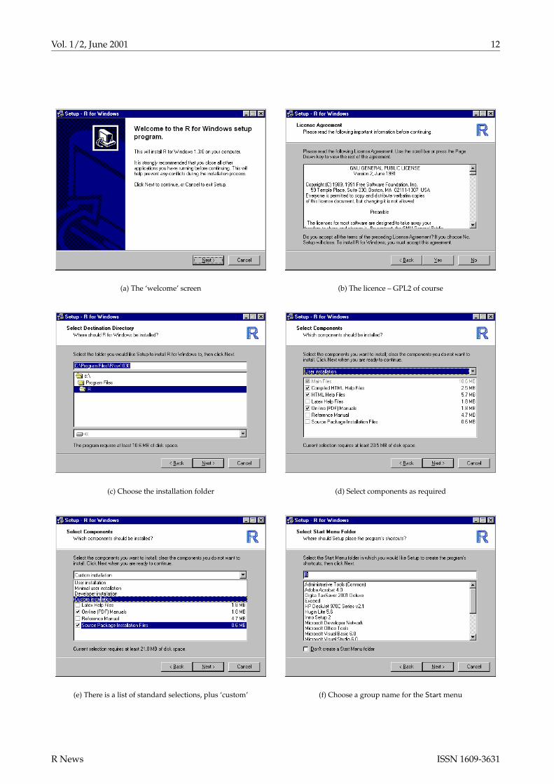
(a) The ‘welcome’ screen (b) The licence – GPL2 of course
(c) Choose the installation folder (d) Select components as required
(e) There is a list of standard selections, plus ‘custom’ (f) Choose a group name for the Start menu
R News ISSN 1609-3631
Vol. 1/2, June 2001 13
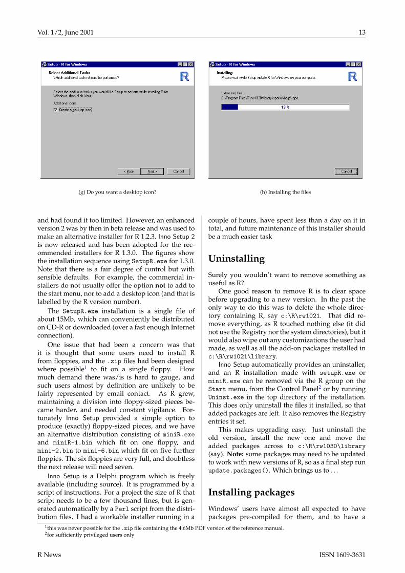
(g) Do you want a desktop icon? (h) Installing the files
and had found it too limited. However, an enhancedversion 2 was by then in beta release and was used tomake an alternative installer for R 1.2.3. Inno Setup 2is now released and has been adopted for the rec-ommended installers for R 1.3.0. The figures showthe installation sequence using SetupR.exe for 1.3.0.Note that there is a fair degree of control but withsensible defaults. For example, the commercial in-stallers do not usually offer the option not to add tothe start menu, nor to add a desktop icon (and that islabelled by the R version number).
The SetupR.exe installation is a single file ofabout 15Mb, which can conveniently be distributedon CD-R or downloaded (over a fast enough Internetconnection).
One issue that had been a concern was thatit is thought that some users need to install Rfrom floppies, and the .zip files had been designedwhere possible1 to fit on a single floppy. Howmuch demand there was/is is hard to gauge, andsuch users almost by definition are unlikely to befairly represented by email contact. As R grew,maintaining a division into floppy-sized pieces be-came harder, and needed constant vigilance. For-tunately Inno Setup provided a simple option toproduce (exactly) floppy-sized pieces, and we havean alternative distribution consisting of miniR.exeand miniR-1.bin which fit on one floppy, andmini-2.bin to mini-6.bin which fit on five furtherfloppies. The six floppies are very full, and doubtlessthe next release will need seven.
Inno Setup is a Delphi program which is freelyavailable (including source). It is programmed by ascript of instructions. For a project the size of R thatscript needs to be a few thousand lines, but is gen-erated automatically by a Perl script from the distri-bution files. I had a workable installer running in a
couple of hours, have spent less than a day on it intotal, and future maintenance of this installer shouldbe a much easier task
Uninstalling
Surely you wouldn’t want to remove something asuseful as R?
One good reason to remove R is to clear spacebefore upgrading to a new version. In the past theonly way to do this was to delete the whole direc-tory containing R, say c:\R\rw1021. That did re-move everything, as R touched nothing else (it didnot use the Registry nor the system directories), but itwould also wipe out any customizations the user hadmade, as well as all the add-on packages installed inc:\R\rw1021\library.
Inno Setup automatically provides an uninstaller,and an R installation made with setupR.exe orminiR.exe can be removed via the R group on theStart menu, from the Control Panel2 or by runningUninst.exe in the top directory of the installation.This does only uninstall the files it installed, so thatadded packages are left. It also removes the Registryentries it set.
This makes upgrading easy. Just uninstall theold version, install the new one and move theadded packages across to c:\R\rw1030\library(say). Note: some packages may need to be updatedto work with new versions of R, so as a final step runupdate.packages(). Which brings us to . . .
Installing packages
Windows’ users have almost all expected to havepackages pre-compiled for them, and to have a
1this was never possible for the .zip file containing the 4.6Mb PDF version of the reference manual.2for sufficiently privileged users only
R News ISSN 1609-3631
Vol. 1/2, June 2001 14
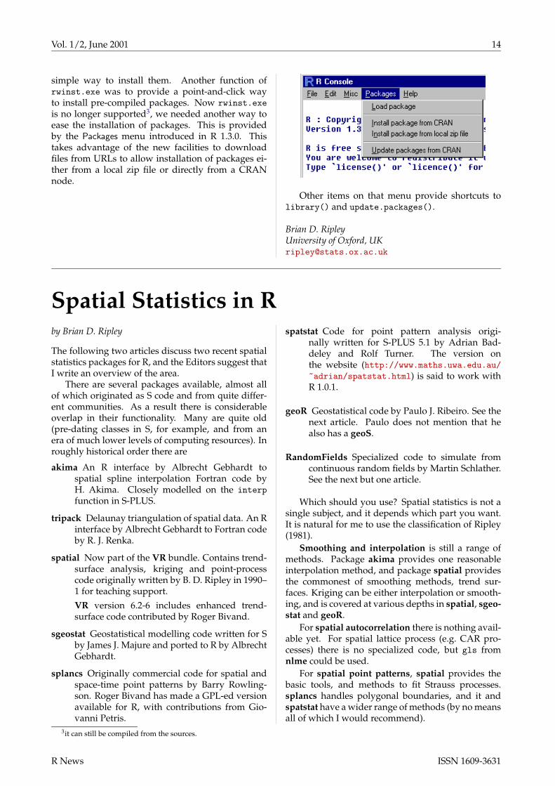
simple way to install them. Another function ofrwinst.exe was to provide a point-and-click wayto install pre-compiled packages. Now rwinst.exeis no longer supported3, we needed another way toease the installation of packages. This is providedby the Packages menu introduced in R 1.3.0. Thistakes advantage of the new facilities to downloadfiles from URLs to allow installation of packages ei-ther from a local zip file or directly from a CRANnode.
Other items on that menu provide shortcuts tolibrary() and update.packages().
Brian D. RipleyUniversity of Oxford, [email protected]
Spatial Statistics in Rby Brian D. Ripley
The following two articles discuss two recent spatialstatistics packages for R, and the Editors suggest thatI write an overview of the area.
There are several packages available, almost allof which originated as S code and from quite differ-ent communities. As a result there is considerableoverlap in their functionality. Many are quite old(pre-dating classes in S, for example, and from anera of much lower levels of computing resources). Inroughly historical order there are
akima An R interface by Albrecht Gebhardt tospatial spline interpolation Fortran code byH. Akima. Closely modelled on the interpfunction in S-PLUS.
tripack Delaunay triangulation of spatial data. An Rinterface by Albrecht Gebhardt to Fortran codeby R. J. Renka.
spatial Now part of the VR bundle. Contains trend-surface analysis, kriging and point-processcode originally written by B. D. Ripley in 1990–1 for teaching support.VR version 6.2-6 includes enhanced trend-surface code contributed by Roger Bivand.
sgeostat Geostatistical modelling code written for Sby James J. Majure and ported to R by AlbrechtGebhardt.
splancs Originally commercial code for spatial andspace-time point patterns by Barry Rowling-son. Roger Bivand has made a GPL-ed versionavailable for R, with contributions from Gio-vanni Petris.
spatstat Code for point pattern analysis origi-nally written for S-PLUS 5.1 by Adrian Bad-deley and Rolf Turner. The version onthe website (http://www.maths.uwa.edu.au/~adrian/spatstat.html) is said to work withR 1.0.1.
geoR Geostatistical code by Paulo J. Ribeiro. See thenext article. Paulo does not mention that healso has a geoS.
RandomFields Specialized code to simulate fromcontinuous random fields by Martin Schlather.See the next but one article.
Which should you use? Spatial statistics is not asingle subject, and it depends which part you want.It is natural for me to use the classification of Ripley(1981).
Smoothing and interpolation is still a range ofmethods. Package akima provides one reasonableinterpolation method, and package spatial providesthe commonest of smoothing methods, trend sur-faces. Kriging can be either interpolation or smooth-ing, and is covered at various depths in spatial, sgeo-stat and geoR.
For spatial autocorrelation there is nothing avail-able yet. For spatial lattice process (e.g. CAR pro-cesses) there is no specialized code, but gls fromnlme could be used.
For spatial point patterns, spatial provides thebasic tools, and methods to fit Strauss processes.splancs handles polygonal boundaries, and it andspatstat have a wider range of methods (by no meansall of which I would recommend).
3it can still be compiled from the sources.
R News ISSN 1609-3631
Vol. 1/2, June 2001 15
It is worth mentioning the commercial moduleS+SpatialStats for S-PLUS, which covers all the ar-eas mentioned here, and is not available for R. Theprospect of such a module, and later of further de-velopment of it, has dampened enthusiasm for user-contributed spatial statistics code over much of thelast decade. It is worth bearing in mind that a greatdeal of the current wealth of packages for R emanatesfrom the work of users filling gaps they saw in S andits commercial offspring.
Bibliography
[1] B. D. Ripley. Spatial Statistics. Wiley, 1981.
Brian D. RipleyUniversity of Oxford, [email protected]
geoR: A Package for GeostatisticalAnalysisby Paulo J. Ribeiro Jr and Peter J. Diggle
geoR is a package to perform geostatistical data anal-ysis and spatial prediction, expanding the set of cur-rently available methods and tools for analysis ofspatial data in R. It has been developed at the De-partment of Mathematics and Statistics, LancasterUniversity, UK. A web site with further informationcan be found at: http://www.maths.lancs.ac.uk/~ribeiro/geoR.html.
Preliminary versions have been available on theweb for the last two years. Based on users’ feedbackand on our own experiences, we judge that the pack-age has been used mainly to support teaching ma-terial and to carry out data analysis and simulationstudies for scientific publications.
Package geoR differs from the other R tools forgeostatistical data analysis in following the model-based inference methods described in (3).
Spatial statistics and geostatistics
Spatial statistics is the collection of statistical methodsin which spatial locations play an explicit role in theanalysis of data. The main aim of geostatistics is tomodel continuous spatial variation assuming a basicstructure of the type Y(x) : x ∈ Rd, d = 1, 2 or 3 for arandom variable Y of interest over a region. Charac-teristic features of geostatistical problems are:
• data consist of responses Yi associated with loca-tions xi which may be non-stochastic, specifiedby the sampling design (e.g. a lattice coveringthe observation region A), or stochastic but se-lected independently of the process Y(x).
• in principle, Y could be determined from anylocation x within a continuous spatial region A.
• {Y(x) : x ∈ A} is related to an unobservedstochastic process {S(x) : x ∈ A}, which wecall the signal.
• scientific objectives include prediction of oneor more functionals of the stochastic process{S(x) : x ∈ A}.
Geostatistics has its origins in problems con-nected with estimation of reserves in mineral ex-ploration/mining (5). Its subsequent development,initially by Matheron and colleagues at École desMines, Fontainebleau (8) was largely independentof “mainstream” spatial statistics. The term “krig-ing” was introduced to describe the resulting meth-ods for spatial prediction. Earlier developments in-clude work by Matérn (6, 7) and by Whittle (10). Rip-ley (9) re-casts kriging in the terminology of stochas-tic process prediction, and this was followed by sig-nificant cross-fertilisation during 1980’s and 1990’s(eg the variogram is now a standard statistical toolfor analysing correlated data in space and/or time).However, there is still vigorous debate on practicalissues such as how to perform inference and predic-tion, and the role of explicit probability models.
The Gaussian model
The currently available functions on geoR assume abasic model specified by:
1. a signal S(·) which is a stationary Gaussianprocess with
(a) E[S(x)] = 0,
(b) Var{S(x)} = σ2,
(c) Corr{S(x), S(x− u)} = ρ(u);
2. the conditional distribution of Yi given S(·) isGaussian with mean µ+ S(xi) and variance τ2;
3. Yi : i = 1, . . . , n are mutually independent, con-ditional on S(·).
R News ISSN 1609-3631
Vol. 1/2, June 2001 16
Covariate information can be incorporated by as-suming a non-constant mean µ = Fβ where F is amatrix with elements of the type f j(xi), a measure-ment of the jth covariate at the ith location. The modelcan be made more flexible by incorporating the fam-ily of Box-Cox transformations (1), in which case theGaussian model is assumed to hold for a transforma-tion of the variable Y.
The basic model parameters are:
• β, the mean parameters,
• σ2, the variance of the signal,
• τ2, the variance of the noise,
• φ, the scale parameter of the correlation func-tion.
Extra parameters provide greater flexibility:
• κ is an additional parameter, required by somemodels for correlation functions, which con-trols the smoothness of the field,
• (ψA,ψR) allows for geometric anisotropy,
• λ is the the Box-Cox transformation parameter.
Package features
The main features of the package are il-lustrated in the PDF document installed at‘geoR/docs/geoRintro.pdf’.
−200 −100 0 100
−20
0−
100
010
020
0
Coord X
Coo
rd Y
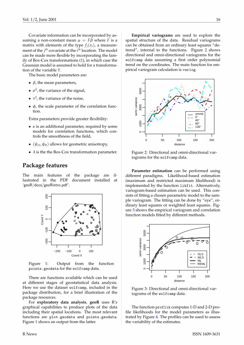
Figure 1: Output from the functionpoints.geodata for the wolfcamp data.
There are functions available which can be usedat different stages of geostatistical data analysis.Here we use the dataset wolfcamp, included in thepackage distribution, for a brief illustration of thepackage resources.
For exploratory data analysis, geoR uses R’sgraphical capabilities to produce plots of the dataincluding their spatial locations. The most relevantfunctions are plot.geodata and points.geodata.Figure 1 shows an output from the latter.
Empirical variograms are used to explore thespatial structure of the data. Residual variogramscan be obtained from an ordinary least squares “de-trend”, internal to the functions. Figure 2 showsdirectional and omni-directional variograms for thewolfcamp data assuming a first order polynomialtrend on the coordinates. The main function for em-pirical variogram calculation is variog.
0 50 100 150 2000
1000
3000
5000
distance
sem
i−va
rianc
e
omnid.0°45°90°135°
Figure 2: Directional and omni-directional var-iograms for the wolfcamp data.
Parameter estimation can be performed usingdifferent paradigms. Likelihood-based estimation(maximum and restricted maximum likelihood) isimplemented by the function likfit. Alternatively,variogram-based estimation can be used. This con-sists of fitting a chosen parametric model to the sam-ple variogram. The fitting can be done by “eye”, or-dinary least squares or weighted least squares. Fig-ure 3 shows the empirical variogram and correlationfunction models fitted by different methods.
0 50 100 150 200
010
0030
0050
00
distance
sem
i−va
rianc
e
OLSWLSMLREML
Figure 3: Directional and omni-directional var-iograms of the wolfcamp data.
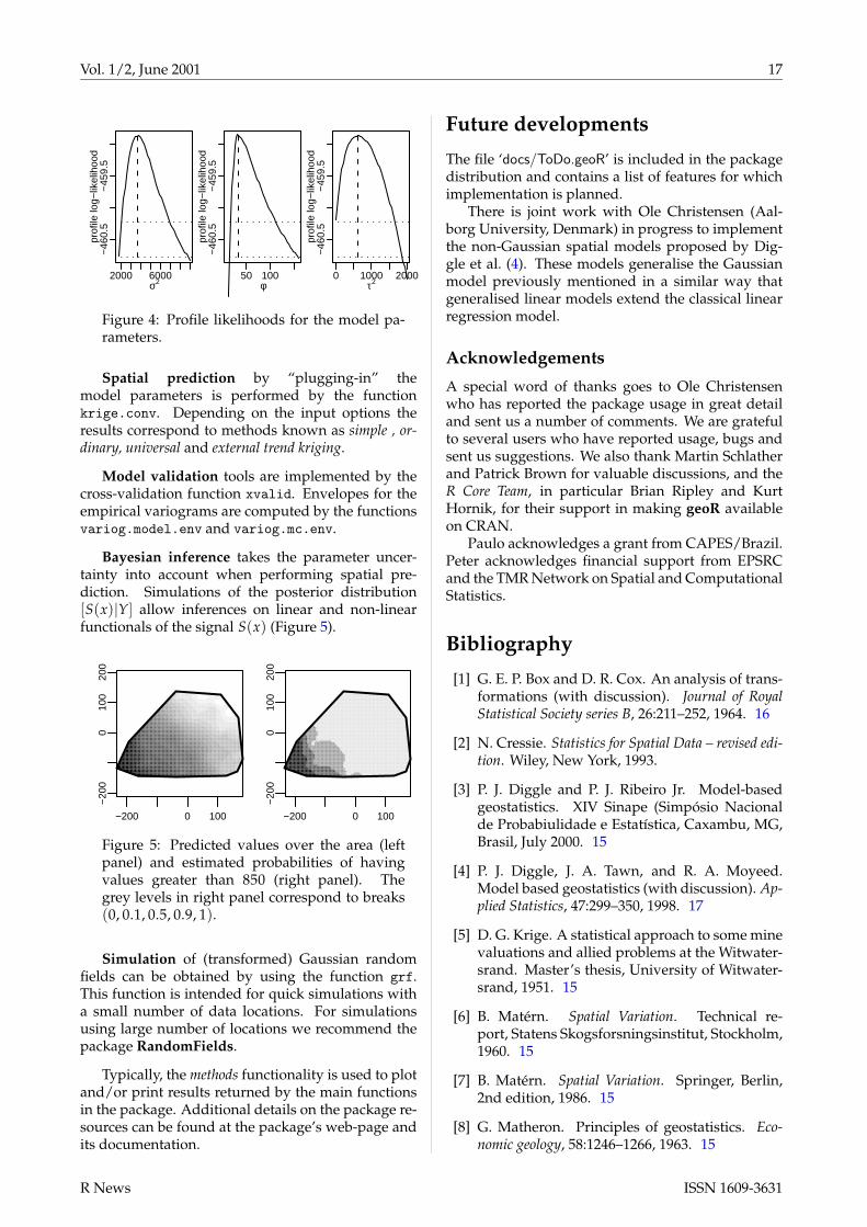
The function proflik computes 1-D and 2-D pro-file likelihoods for the model parameters as illus-trated by Figure 4. The profiles can be used to assessthe variability of the estimates.
R News ISSN 1609-3631
Vol. 1/2, June 2001 17
2000 6000
−46
0.5
−45
9.5
σ2
prof
ile lo
g−lik
elih
ood
50 100
−46
0.5
−45
9.5
φ
prof
ile lo
g−lik
elih
ood
0 1000 2000
−46
0.5
−45
9.5
τ2
prof
ile lo
g−lik
elih
ood
Figure 4: Profile likelihoods for the model pa-rameters.
Spatial prediction by “plugging-in” themodel parameters is performed by the functionkrige.conv. Depending on the input options theresults correspond to methods known as simple , or-dinary, universal and external trend kriging.
Model validation tools are implemented by thecross-validation function xvalid. Envelopes for theempirical variograms are computed by the functionsvariog.model.env and variog.mc.env.
Bayesian inference takes the parameter uncer-tainty into account when performing spatial pre-diction. Simulations of the posterior distribution[S(x)|Y] allow inferences on linear and non-linearfunctionals of the signal S(x) (Figure 5).
−200 0 100
−20
00
100
200
−200 0 100
−20
00
100
200
Figure 5: Predicted values over the area (leftpanel) and estimated probabilities of havingvalues greater than 850 (right panel). Thegrey levels in right panel correspond to breaks(0, 0.1, 0.5, 0.9, 1).
Simulation of (transformed) Gaussian randomfields can be obtained by using the function grf.This function is intended for quick simulations witha small number of data locations. For simulationsusing large number of locations we recommend thepackage RandomFields.
Typically, the methods functionality is used to plotand/or print results returned by the main functionsin the package. Additional details on the package re-sources can be found at the package’s web-page andits documentation.
Future developments
The file ‘docs/ToDo.geoR’ is included in the packagedistribution and contains a list of features for whichimplementation is planned.
There is joint work with Ole Christensen (Aal-borg University, Denmark) in progress to implementthe non-Gaussian spatial models proposed by Dig-gle et al. (4). These models generalise the Gaussianmodel previously mentioned in a similar way thatgeneralised linear models extend the classical linearregression model.
Acknowledgements
A special word of thanks goes to Ole Christensenwho has reported the package usage in great detailand sent us a number of comments. We are gratefulto several users who have reported usage, bugs andsent us suggestions. We also thank Martin Schlatherand Patrick Brown for valuable discussions, and theR Core Team, in particular Brian Ripley and KurtHornik, for their support in making geoR availableon CRAN.
Paulo acknowledges a grant from CAPES/Brazil.Peter acknowledges financial support from EPSRCand the TMR Network on Spatial and ComputationalStatistics.
Bibliography
[1] G. E. P. Box and D. R. Cox. An analysis of trans-formations (with discussion). Journal of RoyalStatistical Society series B, 26:211–252, 1964. 16
[2] N. Cressie. Statistics for Spatial Data – revised edi-tion. Wiley, New York, 1993.
[3] P. J. Diggle and P. J. Ribeiro Jr. Model-basedgeostatistics. XIV Sinape (Simpósio Nacionalde Probabiulidade e Estatística, Caxambu, MG,Brasil, July 2000. 15
[4] P. J. Diggle, J. A. Tawn, and R. A. Moyeed.Model based geostatistics (with discussion). Ap-plied Statistics, 47:299–350, 1998. 17
[5] D. G. Krige. A statistical approach to some minevaluations and allied problems at the Witwater-srand. Master’s thesis, University of Witwater-srand, 1951. 15
[6] B. Matérn. Spatial Variation. Technical re-port, Statens Skogsforsningsinstitut, Stockholm,1960. 15
[7] B. Matérn. Spatial Variation. Springer, Berlin,2nd edition, 1986. 15
[8] G. Matheron. Principles of geostatistics. Eco-nomic geology, 58:1246–1266, 1963. 15
R News ISSN 1609-3631
Vol. 1/2, June 2001 18
[9] B. D. Ripley. Spatial Statistics. Wiley, 1981. 15
[10] P. Whittle. On stationary processes in the plane.Biometrika, 41:434–449, 1954. 15
Paulo J. Ribeiro JrUniversidade Federal do Paraná, Brasil
and Lancaster University, [email protected]
Peter J. DiggleLancaster University, [email protected]
Simulation and Analysis of RandomFieldsby Martin Schlather
Random fields are the d-dimensional analogues ofthe one-dimensional stochastic processes; they areused to model spatial data as observed in environ-mental, atmospheric, and geological sciences. Theyare traditionally needed in mining and exploration tomodel ore deposits, oil reservoirs, and related struc-tures.
The contributed package RandomFields allowsfor the simulation of Gaussian random fields definedon Euclidean spaces up to dimension 3. It includessome geostatistical tools and algorithms for the sim-ulation of extreme-value random fields.
In the following two sections we give an exampleof an application, and a summary of the features ofRandomFields.
A brief geostatistical analysis
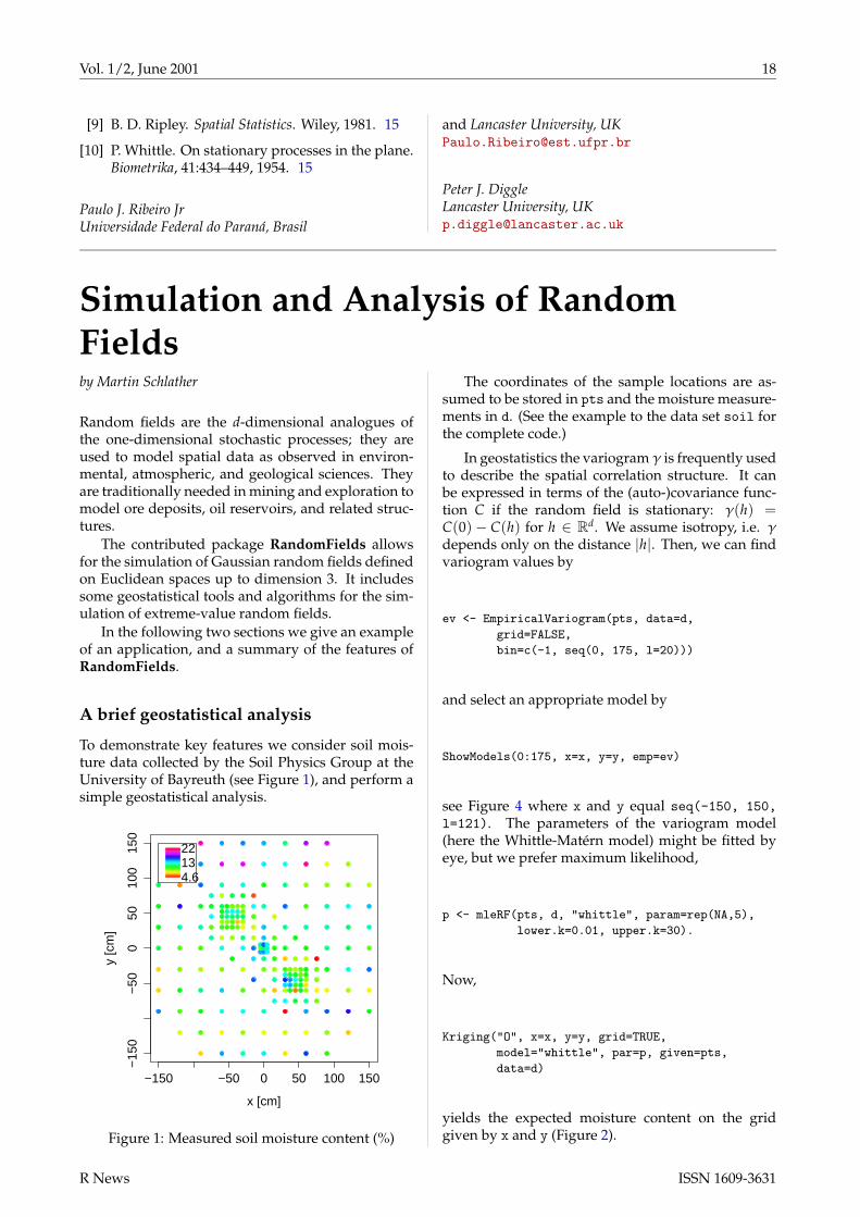
To demonstrate key features we consider soil mois-ture data collected by the Soil Physics Group at theUniversity of Bayreuth (see Figure 1), and perform asimple geostatistical analysis.
−150 −50 0 50 100 150
−15
0−
500
5010
015
0
x [cm]
y [c
m]
22134.6
Figure 1: Measured soil moisture content (%)
The coordinates of the sample locations are as-sumed to be stored in pts and the moisture measure-ments in d. (See the example to the data set soil forthe complete code.)
In geostatistics the variogramγ is frequently usedto describe the spatial correlation structure. It canbe expressed in terms of the (auto-)covariance func-tion C if the random field is stationary: γ(h) =C(0)− C(h) for h ∈ Rd. We assume isotropy, i.e. γdepends only on the distance |h|. Then, we can findvariogram values by
ev <- EmpiricalVariogram(pts, data=d,
grid=FALSE,
bin=c(-1, seq(0, 175, l=20)))
and select an appropriate model by
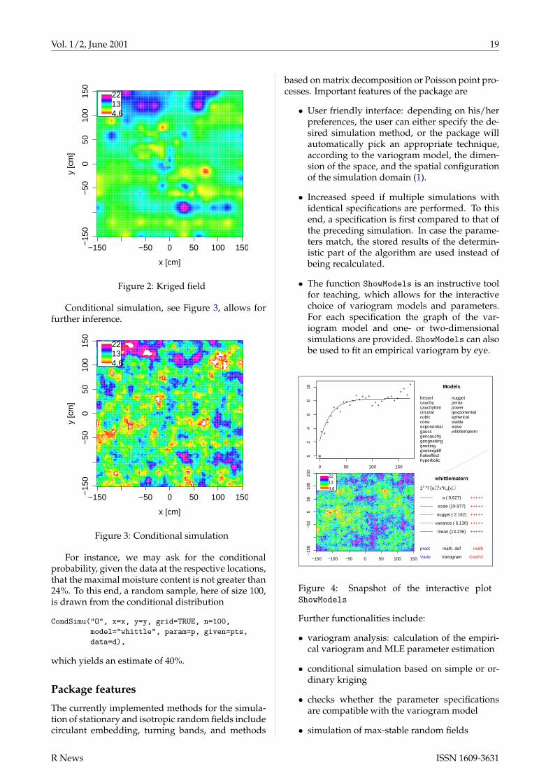
ShowModels(0:175, x=x, y=y, emp=ev)
see Figure 4 where x and y equal seq(-150, 150,l=121). The parameters of the variogram model(here the Whittle-Matérn model) might be fitted byeye, but we prefer maximum likelihood,
p <- mleRF(pts, d, "whittle", param=rep(NA,5),
lower.k=0.01, upper.k=30).
Now,
Kriging("O", x=x, y=y, grid=TRUE,
model="whittle", par=p, given=pts,
data=d)
yields the expected moisture content on the gridgiven by x and y (Figure 2).
R News ISSN 1609-3631
Vol. 1/2, June 2001 19
−150 −50 0 50 100 150−15
0−
500
5010
015
0
x [cm]
y [c
m]
22134.6
Figure 2: Kriged field
Conditional simulation, see Figure 3, allows forfurther inference.
−150 −50 0 50 100 150−15
0−
500
5010
015
0
x [cm]
y [c
m]
22134.6
Figure 3: Conditional simulation
For instance, we may ask for the conditionalprobability, given the data at the respective locations,that the maximal moisture content is not greater than24%. To this end, a random sample, here of size 100,is drawn from the conditional distribution
CondSimu("O", x=x, y=y, grid=TRUE, n=100,
model="whittle", param=p, given=pts,
data=d),
which yields an estimate of 40%.
Package features
The currently implemented methods for the simula-tion of stationary and isotropic random fields includecirculant embedding, turning bands, and methods
based on matrix decomposition or Poisson point pro-cesses. Important features of the package are
• User friendly interface: depending on his/herpreferences, the user can either specify the de-sired simulation method, or the package willautomatically pick an appropriate technique,according to the variogram model, the dimen-sion of the space, and the spatial configurationof the simulation domain (1).
• Increased speed if multiple simulations withidentical specifications are performed. To thisend, a specification is first compared to that ofthe preceding simulation. In case the parame-ters match, the stored results of the determin-istic part of the algorithm are used instead ofbeing recalculated.
• The function ShowModels is an instructive toolfor teaching, which allows for the interactivechoice of variogram models and parameters.For each specification the graph of the var-iogram model and one- or two-dimensionalsimulations are provided. ShowModels can alsobe used to fit an empirical variogram by eye.
Models
besselcauchycauchytbmcircularcubicconeexponentialgaussgencauchygengneitinggneitinggneitingdiffholeeffecthyperbolic
nuggetpentapowerqexponentialsphericalstablewavewhittlematern
*
* *
**
* **
* **
**
** * *
**
** * * *
* *
**
*
*
0 50 100 150
02
46
810
* whittlematern *
21−aΓ(a)−1xaKa(x)
Vario
pract
−−−−−
−−−−−
−−−−−
−−−−−
−−−−−
CovFct
math
+++++
+++++
+++++
+++++
+++++
Variogram
math. def
mean (13.236)
variance ( 6.130)
nugget ( 2.162)
scale (19.977)
a ( 0.527)
0 50 100 150
02
46
810
*
* *
**
* **
* **
**
** * *
**
** * * *
* *
**
*
*
−150 −100 −50 0 50 100 150
−15
0−
500
5010
015
0
22134.6
whittlematern
21−aΓ(a)−1xaKa(x)
Vario
pract
−−−−−
−−−−−
−−−−−
−−−−−
−−−−−
CovFct
math
+++++
+++++
+++++
+++++
+++++
Variogram
math. def
mean (13.236)
variance ( 6.130)
nugget ( 2.162)
scale (19.977)
a ( 0.527)
Figure 4: Snapshot of the interactive plotShowModels
Further functionalities include:
• variogram analysis: calculation of the empiri-cal variogram and MLE parameter estimation
• conditional simulation based on simple or or-dinary kriging
• checks whether the parameter specificationsare compatible with the variogram model
• simulation of max-stable random fields
R News ISSN 1609-3631
Vol. 1/2, June 2001 20
Future extensions may provide further simulationalgorithms for Gaussian and non-Gaussian randomfields, and a basic toolbox for the analysis of geosta-tistical and spatial extreme value data.
Use help(RandomFields) to obtain the main manpage. To start with, the examples in help(GaussRF)are recommended.
Acknowledgement. The work has been supportedby the EU TMR network ERB-FMRX-CT96-0095 on“Computational and statistical methods for the anal-ysis of spatial data” and the German Federal Min-istry of Research and Technology (BMFT) grant PTBEO 51-0339476C. The author is thankful to Tilmann
Gneiting, Martin Mächler, and Paulo Ribeiro forhints and discussions.
Bibliography
[1] M. Schlather. An introduction to positive definitefunctions and to unconditional simulation of ran-dom fields. Technical Report ST-99-10, LancasterUniversity, 1999. 19
Martin SchlatherUniversity of Bayreuth, [email protected]
mgcv: GAMs and Generalized RidgeRegression for Rby Simon N. Wood
Generalized Additive Models (GAMs) have becomequite popular as a result of the work of Wahba(1990) and co-workers and Hastie & Tibshirani(1990). Package mgcv provides tools for GAMs andother generalized ridge regression. This article de-scribes how GAMs are implemented in mgcv: inparticular the innovative features intended to im-prove the GAM approach. The package aims toprovide the convenience of GAM modelling in S-PLUS, combined with much improved model se-lection methodology. Specifically, the degrees offreedom for each smooth term in the model arechosen simultaneously as part of model fitting byminimizing the Generalized Cross Validation (GCV)score of the whole model (not just component wisescores). At present mgcv only provides one dimen-sional smooths, but multi-dimensional smooths willbe available from version 0.6, and future releases willinclude anisotropic smooths. GAMs as implementedin mgcv can be viewed as low rank approximationsto (some of) the generalized spline models imple-mented in gss — the idea is to preserve most of thepractical advantages with which elegant underlyingtheory endows the generalized smoothing spline ap-proach, but without the formidable computationalburden that accompanies full gss models of moder-ately large data sets.
GAMs in mgcv
GAMs are represented in mgcv as penalized gen-eralized linear models (GLMs), where each smoothterm of a GAM is represented using an appropriate
set of basis functions and has an associated penaltymeasuring its wiggliness: the weight given to eachpenalty in the penalized likelihood is determined byits “smoothing parameter”. Models are fitted by theusual iteratively re-weighted least squares schemefor GLMs, except that the least squares problem ateach iterate is replaced by a penalized least squaresproblem, in which the set of smoothing parametersmust be estimated alongside the other model param-eters: the smoothing parameters are chosen by GCV.This section will sketch how this is done in a littlemore detail.
A GLM relating a univariate response variable yto a set of explanatory variables x1, x2, . . ., has thegeneral form:
g(µi) = β0 +β1x1i +β2x2i + · · · (9.1)
where E(yi) ≡ µi and the yi are independent ob-servations on r.v.s all from the same member of theexponential family. g is a smooth monotonic “link-function” that allows a useful degree of non-linearityinto the model structure. The βi are model parame-ters: likelihood theory provides the means for esti-mation and inference about them. The r.h.s. of (9.1)is the “linear predictor” of the GLM, and much of thestatistician’s modelling effort goes into finding an ap-propriate form for this.
The wide applicability of GLMs in part relates tothe generality of the form of the of the linear pre-dictor: the modeller is not restricted to including ex-planatory variables in their original form, but can in-clude transformations of explanatory variables anddummy variables in whatever combinations are ap-propriate. Hence the class of models is very rich, in-cluding, for example, polynomial regression modelsand models for designed experiments. However the
R News ISSN 1609-3631
Vol. 1/2, June 2001 21
standard methods for generalized linear modellingcan become unwieldy as models become more com-plex. In particular, it is sometimes the case that priorbeliefs about appropriate model structure might bestbe summarized as something like:
g(µi) = β0 + s1(x1i) + s2(x2i) + · · · (9.2)
i.e., the linear predictor should be given by a constantplus a smooth function of x1 plus another smoothfunction of x2 and so on (with some side condi-tions on the si to ensure identifiability). It is pos-sible to build this sort of model structure directlywithin the GLM framework using, e.g. polynomialsor more stable bases to represent the smooth terms:but such an approach becomes troublesome as thenumber of smooths and their complexity increases.The two main problems are that model selection be-comes rather cumbersome (many models may needto be compared, and it is not always easy to keepthem nested), and that the basis selected can have arather strong influence on the fitted model (e.g. re-gression splines tend to be rather dependent on knotplacement, while polynomials can be very unstable).
An alternative approach for working with mod-els like (9.2) represents the smooth functions usinglinear smoothers, and performs estimation by back-fitting (Hastie & Tibshirani, 1990) — this has the ad-vantage that a very wide range of smoothers canbe used, but the disadvantage that model selection(choosing the amount of smoothing to perform) isstill difficult.
In mgcv, smooth terms in models like (9.2) arerepresented using penalized regression splines. Thatis, the smooth functions are re-written using a suit-ably chosen set of basis functions, and each has an as-sociated penalty which enables its effective degreesof freedom to be controlled through a single smooth-ing parameter. How this works is best seen throughan example, so consider a model with one linear termand a couple of smooth terms:
g(µi) = β0 +β1x1i + s1(x2i) + s2(x3i) (9.3)
The si can be re-written in terms of basis functionsthus:
s1(x) =k1
∑j=1β j+1b1 j(x) s2(x) =
k2
∑j=1β j+1+k1 b2 j(x)
where ki is the number of basis functions used for si,the β j are parameters to be estimated and the b ji arebasis functions. For example, a suitable set of spline-like basis functions might be:
b j1(x) = x and b ji(x) = |x− x∗ji|3 for i > 1
where the x∗ji are a set of “knots” spread “nicely”throughout the relevant range of explanatory vari-able values. So (9.3) now becomes:
g(µi) = β0 +β1x1i +β2x2i +β3|x2i − x∗22|3 + · · ·
. . . a GLM. If we write the vector of values of g(µi)as η then it’s pretty clear that the previous equa-tion written out for all i can be written as η = Xβ,where the model matrix X follows in an obvious wayfrom the above equation. (Note that mgcv actuallyuses a different (but equivalent) regression spline ba-sis based on cubic Hermite polynomials: its parame-ters are usefully interpretable and it is computation-ally convenient, but rather long winded to write out.)So far the degrees of freedom associated with eachsmooth term are determined entirely by the ki so thatmodel selection will have all the difficulties alludedto above and the fitted model will tend to show char-acteristics dependent on knot locations. To avoidthese difficulties mgcv uses a relatively high valuefor each ki and controls the smoothness (and hencedegrees of freedom) for each term through a set ofpenalties applied to the likelihood of the GLM. Thepenalties measure the wiggliness of each si as:∫
[s′′i (x)]2dx
Since s′′1 (x) = ∑k1j=1 β j+1b′′1 j(x), it’s not hard to see that
it is possible to write:∫[s′′1 (x)]2dx = βTS1β
where β is the parameter vector, and S1 is a posi-tive semi-definite matrix depending only on the ba-sis functions. A similar result applies to s2. So themodel βi’s can be estimated by minimizing:
−l(β) +2
∑i=1λiβ
TSiβ
where l is the log-likelihood for β, and the λi’s con-trol the relative weight given to the conflicting goalsof good fit and model smoothness. Given λi it isstraightforward to solve this problem by (penalized)IRLS, but the λi need to be estimated, and this is notso straightforward.
Recall that the IRLS method for a GLM consistsof iterating the following steps to convergence:
1. The current estimate of β, β[k], yields estimatesof µ and the variance of each yi: Vi. Hence us-ing the current estimates, calculate the follow-ing: (i) the diagonal weight matrix W where:
Wii = [g′(µi)2Vi]−1
and (ii) the vector of pseudodata:
z = Xβ+ Γ(y−µ)
where Γ is a diagonal matrix and Γii =[g′(µi)]−1.
R News ISSN 1609-3631
Vol. 1/2, June 2001 22
2. Minimize:
‖W1/2(z− Xβ)‖2
w.r.t. β to get β[k+1].
mgcv fits GAMs by replacing step 2. with the fol-lowing:
2. Find the λi minimizing:
‖W1/2(z− Xβ)‖2
[tr(I−A)]2 (9.4)
where β is the solution to the problem of mini-mizing:
‖W1/2(z− Xβ)‖2 + ∑ λ jβTS jβ
w.r.t. β, and A is the “influence” or “hat”matrix: X(XTWX + ∑ λ jβ
TS jβ)−1XTW, whosetrace gives the estimated degrees of freedomfor the model.
(9.4) is the GCV score for the model and its effi-cient minimization is the key to the approach used inmgcv: the method for doing this is based on a gen-eralization of the method developed by Gu & Wahba(1991) for generalized smoothing spline models, andis described in Wood (2000). The computational bur-den is cubic in the dimension of β — which is usu-ally much less than the computational burden of us-ing Gu and Wahba’s method for gss models, whichis necessarily cubic in the number of data.
Note that direct minimization of (9.4) is not thesame as minimizing separate GCV scores as part ofeach back-fitting iteration — the latter approach isvery difficult to justify on other than ad hoc grounds.
A simple Bayesian argument yields a covariancematrix estimate for β̂ and hence estimated Bayesianconfidence intervals for the components of the GAM(Wood, 2000; Hastie & Tibshirani, 1990). These aresimilar in spirit to the intervals for smoothing splinesin Wahba (1983).
Note then, that the key point about mgcv is thatthe selection of degrees of freedom for the compo-nents of a fitted GAM is an integral part of modelfitting. Furthermore the manner in which it is in-tegrated is designed to make inclusion of multi-dimensional and anisotropic smooths quite straight-forward. In addition it should be clear that inprinciple any smooth constructed using a basis andquadratic penalty could be incorporated into mgcv’sGAM modelling tools.
Practical GAMs
Because of the way in which estimation of degrees offreedom is integrated into model fitting, the gam()function provided by mgcv is not an exact cloneof what is described in the white book and imple-mented in S-PLUS. This section describes what is im-plemented and how to use it.
gam()
mgcv’s gam() function fits a GAM specified by amodel formula and family, to univariate responsedata. A simple example of its use is:
> gam(y ~ s(x))
which will cause the model:
yi ∼ f (xi) +εi , εi i.i.d. N(0,σ2)
to be estimated, where f is a smooth function.A more complicated example, illustrating a few
more features is:
> gam(y^0.5 ~ -1 + x + s(z,5|f) + s(w) + s(v,20),
data = mydata, family = gamma(link=I))
In this case the response is√
y, and the linear pre-dictor is made up of a linear term in x plus smoothfunctions of z, w and v, with no intercept term. Thedata are assumed to follow a gamma distribution,and the link is the identity function. The 3 differ-ent forms of s() each relate to a different represen-tation of the smooth concerned. s(z,5|f) indicatesthat the smooth function of z is to be represented asa pure un-penalized regression spline, with 5 knots— under the representation used by mgcv this cor-responds to exactly 4 degrees of freedom (‘|f’ indi-cates f ixed degrees of freedom). s(w) indicates thatthe smooth function of w is to be represented usinga default 10 knot penalized regression spline: corre-sponding to maximum degrees of freedom of 9 forthis term. Finally s(v,20) indicates that the smoothof v is to be represented by a 20 knot penalized re-gression spline: this term is being allowed a maxi-mum of 19 degrees of freedom — presumably the re-lationship between
√y and v is expected to be fairly
complicated.The choice of the number of knots is not very crit-
ical, but should be somewhat larger than the esti-mated degrees of freedom plus 1, otherwise: (i) thechoice of knot locations will begin to have a visibleeffect on the shape of the estimated function, and(ii) it is possible that if the GCV function is a strangeshape then the optimization path to the GCV mini-mum may pass beyond the upper boundary on de-grees of freedom, so that the smoothing parameterestimates become incorrectly stuck at that boundary.In practice I usually start with the default 10 knotsplines, but increase the number of knots for anyterms that are then estimated to have close to the cor-responding maximum 9 degrees of freedom.
Other arguments to gam() will be familiar tousers of lm() and glm(). The exception is the ar-gument scale. If the scale parameter for the modeldistribution is known then there is an argument
R News ISSN 1609-3631
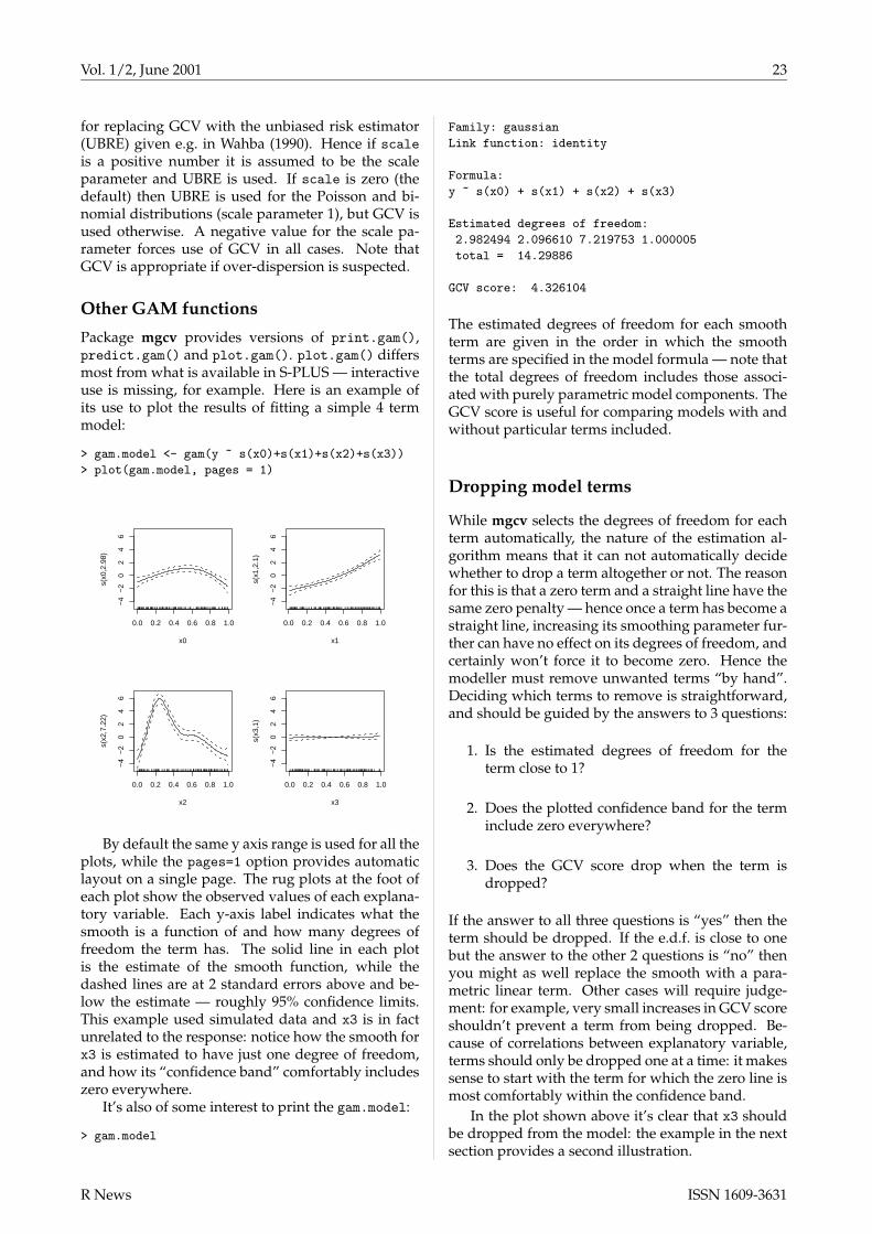
Vol. 1/2, June 2001 23
for replacing GCV with the unbiased risk estimator(UBRE) given e.g. in Wahba (1990). Hence if scaleis a positive number it is assumed to be the scaleparameter and UBRE is used. If scale is zero (thedefault) then UBRE is used for the Poisson and bi-nomial distributions (scale parameter 1), but GCV isused otherwise. A negative value for the scale pa-rameter forces use of GCV in all cases. Note thatGCV is appropriate if over-dispersion is suspected.
Other GAM functions
Package mgcv provides versions of print.gam(),predict.gam() and plot.gam(). plot.gam() differsmost from what is available in S-PLUS — interactiveuse is missing, for example. Here is an example ofits use to plot the results of fitting a simple 4 termmodel:
> gam.model <- gam(y ~ s(x0)+s(x1)+s(x2)+s(x3))
> plot(gam.model, pages = 1)
0.0 0.2 0.4 0.6 0.8 1.0
−4
−2
02
46
x0
s(x0
,2.9
8)
0.0 0.2 0.4 0.6 0.8 1.0
−4
−2
02
46
x1
s(x1
,2.1
)
0.0 0.2 0.4 0.6 0.8 1.0
−4
−2
02
46
x2
s(x2
,7.2
2)
0.0 0.2 0.4 0.6 0.8 1.0
−4
−2
02
46
x3
s(x3
,1)
By default the same y axis range is used for all theplots, while the pages=1 option provides automaticlayout on a single page. The rug plots at the foot ofeach plot show the observed values of each explana-tory variable. Each y-axis label indicates what thesmooth is a function of and how many degrees offreedom the term has. The solid line in each plotis the estimate of the smooth function, while thedashed lines are at 2 standard errors above and be-low the estimate — roughly 95% confidence limits.This example used simulated data and x3 is in factunrelated to the response: notice how the smooth forx3 is estimated to have just one degree of freedom,and how its “confidence band” comfortably includeszero everywhere.
It’s also of some interest to print the gam.model:
> gam.model
Family: gaussian
Link function: identity
Formula:
y ~ s(x0) + s(x1) + s(x2) + s(x3)
Estimated degrees of freedom:
2.982494 2.096610 7.219753 1.000005
total = 14.29886
GCV score: 4.326104
The estimated degrees of freedom for each smoothterm are given in the order in which the smoothterms are specified in the model formula — note thatthe total degrees of freedom includes those associ-ated with purely parametric model components. TheGCV score is useful for comparing models with andwithout particular terms included.
Dropping model terms
While mgcv selects the degrees of freedom for eachterm automatically, the nature of the estimation al-gorithm means that it can not automatically decidewhether to drop a term altogether or not. The reasonfor this is that a zero term and a straight line have thesame zero penalty — hence once a term has become astraight line, increasing its smoothing parameter fur-ther can have no effect on its degrees of freedom, andcertainly won’t force it to become zero. Hence themodeller must remove unwanted terms “by hand”.Deciding which terms to remove is straightforward,and should be guided by the answers to 3 questions:
1. Is the estimated degrees of freedom for theterm close to 1?
2. Does the plotted confidence band for the terminclude zero everywhere?
3. Does the GCV score drop when the term isdropped?
If the answer to all three questions is “yes” then theterm should be dropped. If the e.d.f. is close to onebut the answer to the other 2 questions is “no” thenyou might as well replace the smooth with a para-metric linear term. Other cases will require judge-ment: for example, very small increases in GCV scoreshouldn’t prevent a term from being dropped. Be-cause of correlations between explanatory variable,terms should only be dropped one at a time: it makessense to start with the term for which the zero line ismost comfortably within the confidence band.
In the plot shown above it’s clear that x3 shouldbe dropped from the model: the example in the nextsection provides a second illustration.
R News ISSN 1609-3631
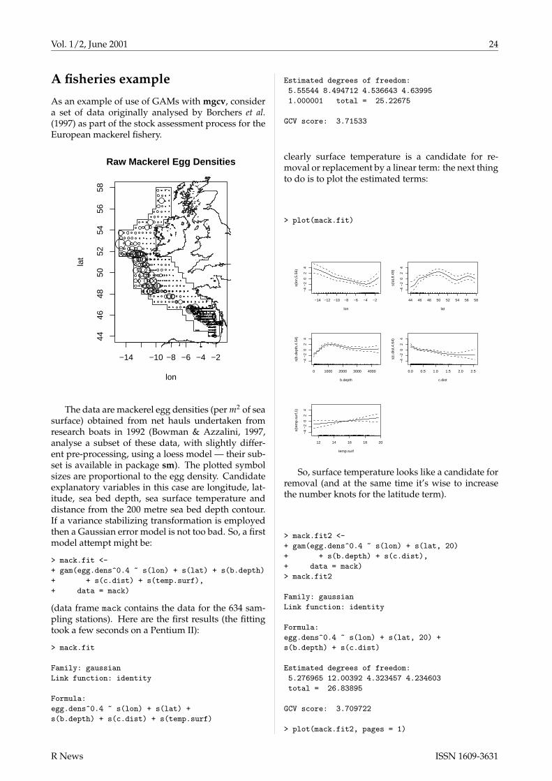
Vol. 1/2, June 2001 24
A fisheries example
As an example of use of GAMs with mgcv, considera set of data originally analysed by Borchers et al.(1997) as part of the stock assessment process for theEuropean mackerel fishery.
−14 −10 −8 −6 −4 −2
4446
4850
5254
5658
Raw Mackerel Egg Densities
lon
lat
The data are mackerel egg densities (per m2 of seasurface) obtained from net hauls undertaken fromresearch boats in 1992 (Bowman & Azzalini, 1997,analyse a subset of these data, with slightly differ-ent pre-processing, using a loess model — their sub-set is available in package sm). The plotted symbolsizes are proportional to the egg density. Candidateexplanatory variables in this case are longitude, lat-itude, sea bed depth, sea surface temperature anddistance from the 200 metre sea bed depth contour.If a variance stabilizing transformation is employedthen a Gaussian error model is not too bad. So, a firstmodel attempt might be:
> mack.fit <-
+ gam(egg.dens^0.4 ~ s(lon) + s(lat) + s(b.depth)
+ + s(c.dist) + s(temp.surf),
+ data = mack)
(data frame mack contains the data for the 634 sam-pling stations). Here are the first results (the fittingtook a few seconds on a Pentium II):
> mack.fit
Family: gaussian
Link function: identity
Formula:
egg.dens^0.4 ~ s(lon) + s(lat) +
s(b.depth) + s(c.dist) + s(temp.surf)
Estimated degrees of freedom:
5.55544 8.494712 4.536643 4.63995
1.000001 total = 25.22675
GCV score: 3.71533
clearly surface temperature is a candidate for re-moval or replacement by a linear term: the next thingto do is to plot the estimated terms:
> plot(mack.fit)
−14 −12 −10 −8 −6 −4 −2−
4−
20
24
lon
s(lo
n,5.
56)
44 46 48 50 52 54 56 58
−4
−2
02
4
lat
s(la
t,8.4
9)
0 1000 2000 3000 4000
−4
−2
02
4
b.depth
s(b.
dept
h,4.
54)
0.0 0.5 1.0 1.5 2.0 2.5
−4
−2
02
4
c.dist
s(c.
dist
,4.6
4)
12 14 16 18 20
−4
−2
02
4
temp.surf
s(te
mp.
surf
,1)
So, surface temperature looks like a candidate forremoval (and at the same time it’s wise to increasethe number knots for the latitude term).
> mack.fit2 <-
+ gam(egg.dens^0.4 ~ s(lon) + s(lat, 20)
+ + s(b.depth) + s(c.dist),
+ data = mack)
> mack.fit2
Family: gaussian
Link function: identity
Formula:
egg.dens^0.4 ~ s(lon) + s(lat, 20) +
s(b.depth) + s(c.dist)
Estimated degrees of freedom:
5.276965 12.00392 4.323457 4.234603
total = 26.83895
GCV score: 3.709722
> plot(mack.fit2, pages = 1)
R News ISSN 1609-3631
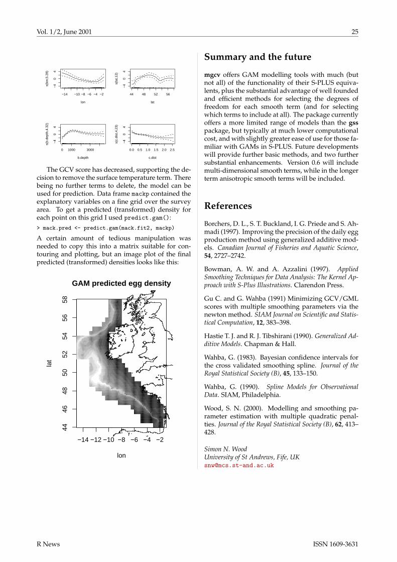
Vol. 1/2, June 2001 25
−14 −10 −8 −6 −4 −2
−4
04
lon
s(lo
n,5.
28)
44 48 52 56
−4
04
lat
s(la
t,12)
0 1000 3000
−4
04
b.depth
s(b.
dept
h,4.
32)
0.0 0.5 1.0 1.5 2.0 2.5
−4
04
c.dist
s(c.
dist
,4.2
3)
The GCV score has decreased, supporting the de-cision to remove the surface temperature term. Therebeing no further terms to delete, the model can beused for prediction. Data frame mackp contained theexplanatory variables on a fine grid over the surveyarea. To get a predicted (transformed) density foreach point on this grid I used predict.gam():> mack.pred <- predict.gam(mack.fit2, mackp)
A certain amount of tedious manipulation wasneeded to copy this into a matrix suitable for con-touring and plotting, but an image plot of the finalpredicted (transformed) densities looks like this:
−14 −12 −10 −8 −6 −4 −2
4446
4850
5254
5658
GAM predicted egg density
lon
latSummary and the future
mgcv offers GAM modelling tools with much (butnot all) of the functionality of their S-PLUS equiva-lents, plus the substantial advantage of well foundedand efficient methods for selecting the degrees offreedom for each smooth term (and for selectingwhich terms to include at all). The package currentlyoffers a more limited range of models than the gsspackage, but typically at much lower computationalcost, and with slightly greater ease of use for those fa-miliar with GAMs in S-PLUS. Future developmentswill provide further basic methods, and two furthersubstantial enhancements. Version 0.6 will includemulti-dimensional smooth terms, while in the longerterm anisotropic smooth terms will be included.
References
Borchers, D. L., S. T. Buckland, I. G. Priede and S. Ah-madi (1997). Improving the precision of the daily eggproduction method using generalized additive mod-els. Canadian Journal of Fisheries and Aquatic Science,54, 2727–2742.
Bowman, A. W. and A. Azzalini (1997). AppliedSmoothing Techniques for Data Analysis: The Kernel Ap-proach with S-Plus Illustrations. Clarendon Press.
Gu C. and G. Wahba (1991) Minimizing GCV/GMLscores with multiple smoothing parameters via thenewton method. SIAM Journal on Scientific and Statis-tical Computation, 12, 383–398.
Hastie T. J. and R. J. Tibshirani (1990). Generalized Ad-ditive Models. Chapman & Hall.
Wahba, G. (1983). Bayesian confidence intervals forthe cross validated smoothing spline. Journal of theRoyal Statistical Society (B), 45, 133–150.
Wahba, G. (1990). Spline Models for ObservationalData. SIAM, Philadelphia.
Wood, S. N. (2000). Modelling and smoothing pa-rameter estimation with multiple quadratic penal-ties. Journal of the Royal Statistical Society (B), 62, 413–428.
Simon N. WoodUniversity of St Andrews, Fife, [email protected]
R News ISSN 1609-3631
Vol. 1/2, June 2001 26
What’s the Point of ‘tensor’?by Jonathan Rougier
One of the packages on CRAN is called tensor, andit exists to compute tensor products of arrays. Thetensor product is a generalisation of the matrix prod-uct, but you can go a lot further if you want: to ex-perience the full power of tensor methods in statis-tics you should consult McCullagh (1987), not for thefaint-hearted.
Tensor notation
In statistics it is often necessary to compute measuresbased on linear combinations of vectors of uncertainquantities. For example, if x and y are uncertain wemight like to know Cov
[Ax, By
]where A and B are
known matrices. In this case we know that the an-swer in matrix-form is A Cov
[x, y
]BT.
Tensors provide an alternative to the matrix-formfor representing linear combinations. The conven-tion with tensors is to use a representitive componentto stand for the whole object, and to let repeated in-dices denote sums of products across objects. Thusinstead of writing v = Ax in matrix-form, we wouldwrite vi = Ai j x j in tensor-form, by which we meanvi = ∑ j ai j x j, for i = 1, . . . , m where A has m rows.
The great advantage of tensors is their trans-parency in use with linear operators. To computeCov
[Ax, By
], for example, first write it as a tensor
then treat everything as scalars:
Cov[Ax, By
]= Cov
[Ai j x j, Bk` y`
]= Ai j Cov
[x j, y`
]Bk`.
To do a tensor calculation the tensor function has toknow what the objects are and what their commonindices are. Using t and %*% would be faster here,but in tensor-form we might do tensor(tensor(A,Cxy, 2, 1), B, 2, 2). The inner call zips up thej index between Ai j and Cov
[x j, y`
], and creates an
object with index set i`, and the outer call zips upthe ` index with Bk` to leave an object with indexset ik. Another way to do the calculation would betensor(A %o% B, Cxy, c(2, 4), c(1, 2)), where‘%o%’ computes the outer product (this is still twotensor products but only one is apparent: the outerproduct is a degenerate tensor product with no sum-ming). This way creates an object with index set i jk`and then zips up j` with Cov
[x j, y`
].
Here’s another example of the transparency oftensor-form. I am always forgetting the expectationof the quadratic form xT Ax in terms of the mean µand variance Σ of x, which, for reference, is usu-ally written E
[xT Ax
]= µT Aµ + tr(AΣ). Write the
quadratic form as a tensor, however, and we see that
E[xT Ax
]= E
[xi Aii′ xi′
]
= Aii′ E[xi xi′
]= Aii′
{µi µi′ + Σii′
}.
So although you might be tempted by t(m) %*%A %*% m + sum(diag(A %*% S)) from the textbook,the smart money is on sum(A * (m %o% m + S)). Wedo not need the tensor function here, but it would betensor(A, m %o% m + S, c(1, 2), c(1, 2)).
Rectangular objects
The greatest strength of tensor-form occurs in thegeneralisation from matrices to arrays. Often un-certain objects possess a rectangular structure, e.g.X =
{xi jk}
might have a natural three-dimensionalstructure. The mean of X is an array of the sameshape as X, while the variance of X is an array withthe same shape as the outer product of X with itself.Thus the variance of Xi jk is, in tensor form, the six-dimensional object
Ci jki′ j′k′ = Cov[Xi jk, Xi′ j′k′
]= E
[xi jk xi′ j′k′
]− E
[xi jk]
E[xi′ j′k′
]where primed indices are used to indicate similarity.
Even if X is two-dimensional (i.e. a matrix), stick-ing with the matrix-form can cause problems. Forexample, to compute Cov
[AXB, X
]we might use the
identity vec(AXB) = (BT ⊗ A) vec X, where ‘⊗’ de-notes the kronecker product and ‘vec X’ creates avector by stacking the columns of X. Originally, thatis why I contributed the function kronecker to R.Then we would have
Cov[
vec(AXB), vec X]= (BT ⊗ A) Var
[vec X
]which requires us to vectorise the naturally two-dimensional object X to give us a two-dimensionalrepresentation of the naturally four-dimensional ob-ject Var
[X]. In tensor-form we would have instead
Cov[Ai j X jk Bkl , X j′k′
]= Ai j Bkl Cov
[X jk, X j′k′
]where Cov
[X jk, X j′k′
]preserves the natural shape of
the variance of X. We might compute this by
tmp <- tensor(tensor(A, varX, 2, 1), B, 2, 1)
aperm(tmp, c(1, 4, 2, 3))
The temporary object tmp has index set i j′k′l whichis permuted using aperm to the set il j′k′. The sameresult could be achieved more spectacularly using
tensor(A %o% B, varX, c(2, 3), c(1, 2))
R News ISSN 1609-3631
Vol. 1/2, June 2001 27
It is often the case that you can arrange for the indexset to come out in the right order, and so remove theneed for a call to aperm.
When the uncertain objects are more than two-dimensional then tensors are usually the only option,both for writing down the required calculation, andperforming it. You can find an example in the Ap-pendix of our forthcoming paper (Craig et al, 2001)which is expressed entirely in tensor-form. In thispaper we have a mixture of one-, two- and three-dimensional objects which are also very large. Forexample, lurking in the Appendix you can find ex-pressions such as
Cov[Bim, Si′′r
]Pi′′ri′′′r′ Hε
i′ i′′′r′(x) gm(x),
a two-dimensional expression (in ii′) which is a func-tion of the vector x. To give you some idea of thescale of this calculation, there are about 60 i’s, 45 m’s,and 6 r’s, and x is 40-dimensional. (We then have tointegrate x out of this, but that’s another story!).
In our current development of this work we willneed to evaluate the object E
[Bim Bi′m′ Bi′′m′′ Bi′′′m′′′
].
This has about 5 × 10¹³ components and so thiscalculation is currently ‘on hold’, but I am hopingthat Luke Tierney’s eagerly anticipated hyper-spatialmemory manager will sort this out and spare mefrom having to thinking too deeply about the essen-tial structure of these objects.
Implementation
Conceptually, a tensor product is a simple thing.Take two arrays A and B, and identify the extents
in each to be collapsed together (make sure theymatch!). Permute the collapse extents of A to the endand the collapse extents of B to the beginning. Thenre-shape both A and B as matrices and take the ma-trix product. Reshape the product to have the non-collapse extents of A followed by the non-collapse ex-tents of B and you are done.
In order for these operations to be efficient, weneed a rapid aperm operation. The aperm functionin R 1.2 was not really fast enough for large objects,and so I originally wrote tensor entirely in C, using aPython approach for arrays called ‘strides’. In R 1.3however, there is a new aperm that itself uses strides,to achieve a reduction in calculation time of about80%. The new version of tensor, version 1.2, there-fore does the obvious thing as outlined above, anddoes it entirely in R. But the old version of tensor,version 1.1-2, might still be useful for dealing withvery large objects, as it avoids the duplication thatcan happen when passing function arguments.
References
P. S. Craig, M. Goldstein, J. C. Rougier and A. H. Se-heult (2001). Bayesian forecasting for complex sys-tems using computer simulators, Journal of the Amer-ican Statistical Association, forthcoming.P. McCullagh (1987). Tensor Methods in Statistics,Chapman and Hall.
Jonathan RougierUniversity of Durham, [email protected]
On Multivariate t and Gauß Probabilitiesin Rby Torsten Hothorn, Frank Bretz and Alan Genz
Introduction
The numerical computation of a multivariate nor-mal or t probability is often a difficult problem. Re-cent developments resulted in algorithms for the fastcomputation of those probabilities for arbitrary cor-relation structures. We refer to the work describedin (3), (4) and (2). The procedures proposed in thosepapers are implemented in package mvtnorm, avail-able at CRAN. Basically, the package implementstwo functions: pmvnorm for the computation of mul-tivariate normal probabilities and pmvt for the com-putation of multivariate t probabilities, in both casesfor arbitrary means (resp. noncentrality parameters),
correlation matrices and hyperrectangular integra-tion regions.
We first illustrate the use of the package using asimple example of the multivariate normal distribu-tion. A little more details are given in Section ‘De-tails’. Finally, an application of pmvt in a multipletesting problem is discussed.
A simple example
Assume that X = (X1, X2, X3) is multivariate normalwith correlation matrix
Σ =
1 35
13
35 1 11
1513
1115 1
R News ISSN 1609-3631
Vol. 1/2, June 2001 28
and expectation µ = (0, 0, 0)>. We are interested inthe probability
P(−∞ < X1 ≤ 1,−∞ < X2 ≤ 4,−∞ < X3 ≤ 2).
This is computed as follows:
R> m <- 3
R> sigma <- diag(3)
R> sigma[2,1] <- 3/5
R> sigma[3,1] <- 1/3
R> sigma[3,2] <- 11/15
R> pmvnorm(lower=rep(-Inf, m), upper=c(1,4,2),
mean=rep(0, m), sigma)
$value
[1] 0.8279847
$error
[1] 5.684033e-07
$msg
[1] "Normal Completion"
The mean vector is passed to pmvnorm by the argu-ment mean, and sigma is the correlation matrix (onlythe lower triangle being used) The region of inte-gration is given by the vectors lower and upper,both can have elements -Inf or +Inf. The value ofpmvnorm is a list with the following components:
value: the estimated integral value,
error: the estimated absolute error,
msg: a status message, indicating whether or not thealgorithm terminated correctly.
From the results above it follows that P(−∞ < X1 ≤1,−∞ < X2 ≤ 4,−∞ < X3 ≤ 2) ≈ 0.82798 with anabsolute error estimate of 2.7× 10⁻⁷.
Details
This section outlines the basic ideas of the algorithmsused. The multivariate t distribution (MVT) is givenby
T(a, b,Σ,ν) =21− ν
2
Γ(ν2 )
∞∫0
sν−1e−s22 Φ
(sa√ν
,sb√ν
,Σ)
ds,
where the multivariate normal distribution function(MVN)
Φ(a, b,Σ) =1√
|Σ|(2π)m
b1∫a1
b2∫a2
. . .bm∫
am
e−12 xtΣ−1xdx,
x = (x1, x2, ..., xm)t, −∞ ≤ ai < bi ≤ ∞ for all i,and Σ is a positive semi-definite symmetric m × mmatrix. The original integral over an arbitrary m-dimensional, possibly unbounded hyper-rectangle istransformed to an integral over the unit hypercube.
These transformations are described in (3) for theMVN case and in (2) for the MVT case. Several suit-able standard integration routines can be applied tothis transformed integral. For the present implemen-tation randomized lattice rules were used. Such lat-tice rules seek to fill the integration region evenly ina deterministic process. In principle, they constructregular patterns, such that the projections of the in-tegration points onto each axis produce an equidis-tant subdivision of the axis. Robust integration errorbounds are obtained by introducing additional shiftsof the entire set of integration nodes in random di-rections. Since this additional randomization step isonly performed to introduce a robust Monte Carloerror bound, 10 simulation runs are usually suffi-cient. For a more detailed description (2) might bereferred to.
Applications
The multivariate t distribution is applicable in a widefield of multiple testing problems. We will illus-trate this using a example studied earlier by (1). Forshort, the effects of 5 different perfusates in capil-lary permeability in cats was investigated by (5). Thedata met the assumptions of a standard one-factorANOVA. For experimental reasons, the investigatorswere interested in a simultaneous confidence inter-vals for the following pairwise comparisons: β1 −β2,β1 −β3,β1 −β5,β4 −β2 and β4 −β3. Therefore,the matrix of contrast is given by
C =
1 −1 0 0 01 0 −1 0 01 0 0 0 −10 1 0 −1 00 0 1 −1 0
.
Reference (1) assumed that β = (β1, . . . ,β5) is mul-tivariate normal with mean β and covariance matrixσ2V, where V is known. Under the null hypothesisβ = 0, we need knowledge about the distribution ofthe statistic
W = max1≤ j≤5
|c j(β̂−β)|
σ̂√
c jVc>j
where c j is the jth row of C. By assumption, σ̂is χν distributed, so under hypothesis W the ar-gument to max follows a multivariate t distribu-tion. Confidence intervals can be obtained by c jβ̂±wασ̂
√c jVc>i , where wα is the 1 −α quantile of the
null distribution of W. Using pmvt, one can easilycompute the quantile for the example cited above.
R> n <- c(26, 24, 20, 33, 32)
R> V <- diag(1/n)
R> df <- 130
R> C <- c(1,1,1,0,0,-1,0,0,1,0,0,-1,0,0,
R News ISSN 1609-3631
Vol. 1/2, June 2001 29
1,0,0,0,-1,-1,0,0,-1,0,0)
R> C <- matrix(C, ncol=5)
R> cv <- C %*% V %*% t(C)
R> cr <- matrix(rep(0, ncol(cv)^2),
ncol=ncol(cv))
R> for (i in 1:5) {
for (j in 1:5) {
cr[i,j] <- cv[i,j] / sqrt(cv[i,i]*cv[j,j])
}
}
R> delta <- rep(0,5)
R> myfct <- function(q, alpha) {
lower <- rep(-q, ncol(cv))
upper <- rep(q, ncol(cv))
pmvt(lower, upper, df, cr, delta,
abseps=0.0001)$value - alpha
}
R> round(uniroot(myfct, lower=1, upper=5,
alpha=0.95)$root, 3)
[1] 2.561
Here n is the sample size vector of each level ofthe factor, V is the covariance matrix of β. With thecontrasts C we can compute the correlation matrix crof Cβ. Finally, we are interested in the 95% quantileof W. A wrapper function myfct computes the dif-ference of the multivariate t probability for quantile qand alpha. The alpha quantile can now be computedeasily using uniroot. The 95% quantile of W in thisexample is 2.561; reference (1) obtained 2.562 using80.000 simulation runs. The computation needs 8.06seconds total time on a Pentium III 450 MHz with256 MB memory.
Using package mvtnorm, the efficient computa-tion of multivariate normal or t probabilities is nowavailable in R. We hope that this is helpful to users /programmers who deal with multiple testing prob-lems.
Bibliography
[1] Don Edwards and Jack J. Berry. The efficiency ofsimulation-based multiple comparisons. Biomet-rics, 43:913–928, December 1987. 28, 29
[2] A. Genz and F. Bretz. Numerical computationof multivariate t-probabilities with application topower calculation of multiple contrasts. Journal ofStatistical Computation and Simulation, 63:361–378,1999. 27, 28
[3] Alan Genz. Numerical computation of multivari-ate normal probabilities. Journal of Computationaland Graphical Statistics, 1:141–149, 1992. 27, 28
[4] Alan Genz. Comparison of methods for thecomputation of multivariate normal probabili-ties. Computing Science and Statistics, 25:400–405,1993. 27
[5] P. D. Watson, M. B. Wolf, and I. S. Beck-Montgemery. Blood and isoproterenol reducecapillary permeability in cat hindlimb. The Amer-ican Journal of Physiology, 252:H47–H53, 1987. 28
Torsten HothornFriedrich-Alexander-Universität Erlangen-NürnbergInstitut für Medizininformatik, Biometrie und Epidemi-ologieWaldstraße 6, D-91054 [email protected]
Frank BretzUniversität HannoverLG Bioinformatik, FB GartenbauHerrenhäuser Str. 2D-30419 [email protected]
Alan GenzDepartment of MathematicsWashington State UniversityPullman, WA 99164-3113 [email protected]
The first author gratefully acknowledges support byDeutsche Forschungsgemeinschaft, grant SFB 539 /A4.
Programmer’s NicheEdited by Bill Venables
Save the environment
When you start to learn how to program in S youdon’t have to get very far into it before you find thatthe scoping rules can be rather unintuitive. The sortof difficulty that people first encounter is often some-thing like the following (on S-PLUS 2000):
> twowaymeans <- function(X, f)
apply(X, 2, function(x) tapply(x, f, mean))
> twowaymeans(iris[,1:2], iris$Species)
Error in FUN(X): Object "f" not found
Dumped
The dismay expressed by disappointed neophytes onS-news is often palpable. This is not helped by thepeople who point out that on R it does work becauseof the more natural scoping rules:
> twowaymeans(iris[,1:2], iris$Species)
R News ISSN 1609-3631
Vol. 1/2, June 2001 30
Sepal.Length Sepal.Width
setosa 5.006 3.428
versicolor 5.936 2.770
virginica 6.588 2.974
Some people even claim to have chosen R over S-PLUS for the sake of the scoping rules alone. Strange,but true.
The different scoping rules are just one conse-quence of a feature of R, namely that its functionshave an “environment” attached to them which isusually called the function closure. In S the searchpath is the same for all functions, namely the localframe, frame 1, frame 0 and the sequence of data di-rectories or attached objects. This can be altered onthe fly and functions may be made to look at, and in-terfere with, non-standard places on the search pathbut this is usually regarded as a device strictly for theexcessively brave or the excessively lucky. For some,even using frames 0 or 1 at all is considered ratherreckless.
This is the territory where R and S diverge verymarkedly indeed. How is R so different? I will leavereaders to follow up this interesting story using thestandard references. All I will try to do here is givean extended example that I hope motivates that kindof followup study. In fact I intend to give the “otherstory” that I referred to so tantalizingly in the firstProgrammer’s Niche article, of course.
Function closures
We can think of the function closure as a little scratch-pad attached to the function that initially containssome objects on which its definition may depend.This turns out to be a useful place to put other thingswhich the function needs to have, but which youdon’t want to re-create every time you call the func-tion itself. If you understand the concept of frame 0(the frame of the session) in S, this is a bit like a localframe 0, but for that function alone.
Subsets revisited with caching
In my last article on profiling I used an example of arecursive function to generate all possible subsets ofsize r of a fixed set of size n. The result is an (n
r)× rmatrix whose rows define the subsets. Some timeago I devised a way of speeding this process up inS by storing (or ‘caching’) partial results in frame 0.Doug Bates then pointed out that it could be donemuch more cleanly using function closures in R.
Thinking back on the subset calculation, noticethat if you have all possible subsets of size r of theintegers 1, 2, . . . , n as a matrix then the subsets of anyset of size n stored in a vector v can be got by giving vthe elements of this matrix as an index vector and us-ing the result to fill a similar matrix with the chosenelements of v. (Oh well, think about it for a bit.)
The way we generate all possible subsets of sizer from n involves repeatedly generating all possiblesubsets of smaller sizes from a smaller sets. Whatwe are going to do now is generate these indexingvectors and store them in the the function closure.The index vector for subsets of size 4 from sets ofsize 10, say, will be given the non-standard name,4 10. (It is no penalty to use non-standard nameshere since these objects will always be accessed in-directly.) Then when we need to generate a set ofsubsets we will check to see if the index vector to doit is cached in the environment first. If it is we dothe job by a single index computation; if not we firstgenerate the index by a recursive call and then use it.
Actually it is one of those times when the codeis easier to read than an explanation of it. Howevereven the code is not all that easy. The result, how-ever, is a further spectacular increase in speed but atthe cost of greatly increasing your memory usage. Ifyou have to do this sort of computation repeatedly,though, the advantages of the cached index vectorsin the environment are maintained, of course, so thesecond time round, even for the large number of sub-sets, the computation is nearly instantaneous (pro-viding you are not hitting a memory limit and re-peatedly swapping, swapping, swapping, . . . ). Sothe technique is both interesting and potentially im-portant.
The code
To get a function with an explicit environment (andnot just the global environment) we are going to doit in the “old way” by writing a function to generatethe function itself. OK, here goes:
makeSubsets <- function() {
putenv <- function(name, value)
assign(name, value,
envir = environment(Subsets))
getenv <- function(name)
get(name, envir = environment(Subsets))
thereIsNo <- function(name)
!exists(name, envir = environment(Subsets))
function(n, r, v = 1:n) {
v0 <- vector(mode(v), 0)
if(r < 0 || r > n) stop("incompatible n, r")
sub <- function(n, r, v) {
if(r == 0) v0 else
if(r == n) v[1:n] else {
if(r > 1) {
i1 <- paste(n-1, r-1)
i2 <- paste(n-1, r)
if(thereIsNo(i1))
putenv(i1, sub(n-1, r-1, 1:(n-1)))
if(thereIsNo(i2))
putenv(i2, sub(n-1, r, 1:(n-1)))
m1 <- matrix(v[-1][getenv(i1)],
R News ISSN 1609-3631
Vol. 1/2, June 2001 31
ncol = r-1)
m2 <- matrix(v[-1][getenv(i2)],
ncol = r)
} else {
m1 <- NULL
m2 <- matrix(v[2:n], ncol = 1)
}
rbind(cbind(v[1], m1), m2)
}
}
sub(n, r, v)
}
}
Subsets <- makeSubsets()
The local environment will initially contain the smallutility functions getenv, putenv and thereIsNo fordoing various things with the local environment.Within the function itself the index matrices are re-ferred to by the constructed character strings i1 andi2.
Here are a few little comparisons on my oldishSun system:
## best from last time
> system.time(x <- subsets2(20, 7))
[1] 22.26 3.96 26.29 0.00 0.00
## first time round
> system.time(X <- Subsets(20, 7))
[1] 4.94 0.25 5.38 0.00 0.00
## second time
> system.time(L <- Subsets(20, 7, letters))
[1] 1.90 0.04 2.00 0.00 0.00
These times are actually quite variable and depend alot on what is going on with the machine itself. Notethat with the fastest function we devised last time thecomputation took about 26 seconds total time. Withthe caching version the same computation took 5.38seconds total time the first time and only 2 secondsthe next time when we did the same computationwith a different set.
Compression
There is a final speculative twist to this story that Ican’t resist throwing in even though its usefulnesswill be very machine dependent.
It must be clear that storing oodles of very largeindex vectors in the local environment will incur amemory overhead that might well become a prob-lem. Can we compress the vectors on the fly in anyway to cut down on this? The only way I have beenable to see how to do this has been to use so-called
“run length encoding”. Given a vector, v, the func-tion rle finds the lengths of each run of consecutiveidentical values and returns a list of two components:one giving the values that are repeated in each runand the other the lengths of the runs. This is the in-verse operation to the one performed by rep: if wefeed those two components back to rep we re-createthe original vector.
The function rle is one of the neatest examplesof slick programming around. It is very short anda nice little puzzle to see how it works. Here is acut-down version of it that returns a value with listnames matching the argument names of rep:
rle <- function (x) {
n <- length(x)
y <- x[-1] != x[-n]
i <- c(which(y), n)
list(x = x[i], times = diff(c(0, i)))
}
The thing you notice about these subset index vec-tors (when the subsets are generated in this lexico-graphic order) is that they do have long runs of re-peated values. In fact the run-length encoded ver-sion is an object typically only about half as big (inbytes) as the object itself. This produces a compres-sion of the memory requirements, but at an increasedcomputational cost again, of course. To incorporatethe idea into our makeSubsets function we need toinclude this specialised version of rle in the localenvironment as well and to modify the getting andputting functions to include the encoding and decod-ing:
putenv <- function(name, value)
assign(name, rle(value),
envir = environment(Subsets))
getenv <- function(name)
do.call("rep", get(name,
envir = environment(Subsets)))
No modification to the function itself is needed, andthis is one advantage of using accessor functions todeal with the local environment, of course.
I think this is an interesting idea, but I have to re-port that for all the systems I have tried it upon theincreased computational penalty pretty well elimi-nates the gains made by caching. Quel domage!
Bill VenablesCSIRO Marine Labs, Cleveland, Qld, [email protected]
R News ISSN 1609-3631
Vol. 1/2, June 2001 32
Recent Eventsby Friedrich Leisch
This new regular columns will report about recentevents related to R, S or statistical computing in gen-eral. If you have been to a conference where R turnedout to be one of the hot topics (or simply part ofa nifty software demonstration), please write a fewlines and send them to the editors.
DSC 2001
The second workshop on distributed statistical com-puting took place at the Vienna University of Tech-nology from March 15 to March 17, 2001. As its pre-decessor in 1999 it turned out to be a highly stim-ulating event sparking many discussions on the fu-ture of statistical computing, which continued evenafter dinner and didn’t stop until the last beerswere ordered long after midnight. Of course theworkshop program had a slight bias towards R, but
speakers also included John Eaton (Octave), Gün-ther Sawitzki (Voyager), David Smith (S-PLUS), Deb-orah Swayne (GGobi), Antony Unwin (MANET) andmany more. Please have a look at the homepageof the workshop at http://www.ci.tuwien.ac.at/Conferences/DSC.html to see who participated andwhat topics exactly we talked about. Online proceed-ings are also available as PDF files.
The workshop was followed by two days of openR core meetings, where all interested could partici-pate and discuss future plans for R and S. The twoDSC workshops mark the only two occasions wherealmost the complete R core team has ever met physi-cally, normally we are spread out over 3 continentswith completely incompatible time zones and allwork on R has to be organized virtually using theInternet.
Friedrich LeischTechnische Universität Wien, [email protected]
Editors:Kurt Hornik & Friedrich LeischInstitut für Statistik und WahrscheinlichkeitstheorieTechnische Universität WienWiedner Hauptstraße 8-10/1071A-1040 Wien, Austria
Editor Programmer’s Niche:Bill Venables
Editorial Board:Douglas Bates, John Chambers, Peter Dal-gaard, Robert Gentleman, Stefano Iacus, RossIhaka, Thomas Lumley, Martin Maechler, GuidoMasarotto, Paul Murrell, Brian Ripley, DuncanTemple Lang and Luke Tierney.
R News is a publication of the R project for statistical
computing, communications regarding this publica-tion should be addressed to the editors. All articlesare copyrighted by the respective authors. Pleasesend submissions to the programmer’s niche col-umn to Bill Venables, all other submissions to KurtHornik or Friedrich Leisch (more detailed submis-sion instructions can be found on the R homepage).
R Project Homepage:http://www.R-project.org/
Email of editors and editorial board:firstname.lastname @R-project.org
This newsletter is available online athttp://cran.R-project.org/doc/Rnews/
R News ISSN 1609-3631