Daubechies wavelet coefficients: a tool to study ... · GEOFÍSICA INTERNACIONAL APRIL - JUNE 2014 103 ÀXFWXDWLRQV DUH DQ LPSRUWDQW FRQWULEXWRU WR the large-scale transfer of SW

GEOFÍSICA INTERNACIONAL (2014) 53-2: 101-115

101

ORIGINAL PAPER

Arian Ojeda González*, Odim Mendes Junior, Margarete Oliveira Domingues and Varlei Everton Menconi

Received: September 04, 2012; accepted: August 06, 2013; published on line: April 01, 2014

A. Ojeda González*

O. Mendes JuniorV.E. MenconiDGE/CEANational Institute for Space ResearchINPE 12227-010 São José dos CamposSP, Brazil*Corresponding author: [email protected]

Hemos estudiado un conjunto de 41 nubes magnéticas (MCs) detectadas por el satélite ACE, utilizamos la transformada wavelet ortogonal discreta (usando wavelet de Daubechies de orden dos) en tres regiones: vaina de plasma, nube y posterior a la nube. Trabajamos con datos de las componentes del campo magnético interplanetario (IMF) en el sistema de coordenadas GSM con resolución temporal de 16 s. Se ha elegido como herramienta matemática la media estadística

Dd1 ). Los

han utilizado porque ellos representan la regularidad local presente en la señal de estudio. Los resultados reprodujeron el hecho bien conocido, que la dinámica es mas compleja en la vaina de plasma que en la región de la MC. Esta técnica podría ser útil a un especialista en ayudarlo encontrar fronteras de eventos cuando se trabaja con el IMF, es decir, una mejor forma de visualizar los datos.

facilitar encontrar algunos choques que serían difíciles de detectar por simple inspección visual del IMF. Podemos aprender que las

todas las nubes, en algunos casos las ondas pueden penetrar desde la vaina hasta la MC. Esta metodología aún no ha sido testada para

en el IMF de otros eventos interplanetarios geoefectivos, tales como, regiones de interacción corrotante (CIRs), lámina de corriente heliosférica (HCS) o para ICMEs sin características de MC. Como es la primera vez que esta técnica se aplica a los datos del IMF, opinamos que una de las contribuciones de este trabajo es la presentación de este enfoque a la Comunidad de Físicos Espaciales.

Palabras clave: electrodinámica espacial, nubes magnéticas, análisis de series temporales, transformada wavelet discreta, clima espacial.

We have studied a set of 41 magnetic clouds (MCs) measured by the ACE spacecraft, using the discrete orthogonal wavelet transform (Daubechies wavelet of order two) in three regions: Pre-MC (plasma sheath), MC and Post-MC. We have used data from the IMF GSM-components with time resolution of 16 s. The mathematical property chosen was the

( Dd1have been used because they represent the local regularity present in the signal being studied. The results reproduced the well-known fact that the dynamics of the sheath region is more than that of the MC region. This technique could be useful to help a specialist to

datasets, i.e., a best form to visualize the data.

easy to see in the IMF data by simple visual

are not low in all MCs, in some cases waves can penetrate from the sheath to the MC. This methodology has not yet been tested to

IMF for any other geoeffective interplanetary events, such as Co-rotating Interaction Regions (CIRs), Heliospheric Current Sheet (HCS) or ICMEs without MC signatures. In our

is applied to the IMF data with this purpose, the presentation of this approach for the Space Physics Community is one of the contributions of this work.

Key words: space electrodynamics, magnetic clouds, time series analysis, discrete wavelet transform, space weather.

M. Oliveira DominguesLAC/CTENational Institute for Space ResearchINPE 12227-010 São José dos CamposSP, Brazil

A. Ojeda GonzálezDepartment of Space GeophysicsInstitute of Geophysics and AstronomyIGA Havana City, Cuba

A. Ojeda González, O. Mendes Junior, M. Oliveira Domingues and V. Everton Menconi

102 VOLUME 53 NUMBER 2

One of the very important phenomena in space is the Interplanetary Coronal Mass Ejection (ICME) as a disturbance in the solar wind (SW) that presents a large importance due to its potential geoeffectivity. Physically, a subset of ICMEs has

rotates smoothly through a large angle, and the proton temperature is low (Burlaga et al., 1981; Klein and Burlaga, 1982; Gosling, 1990). Such events, named magnetic clouds (MCs), have received considerable attention, because they are an important source of southward

Investigations on the relation between MCs and geomagnetic storms have been carried out by many researchers (for instance, Burlaga et al., 1981; Klein and Burlaga, 1982; Gonzalez and Tsurutani, 1987; Tsurutani et al., 1988; Tsurutani and Gonzalez, 1992; Farrugia et al., 1995; Lepping et al., 2000; Dal Lago, et al., 2000; Dal Lago et al., 2001; Wu and Lepping, 2002a,b) with many purposes. Echer et al. (2005) studied a total of 149 MCs from 1966 to 2001, where 51 are of the NS type, 83 of the type SN, and 15 unipolar (N or S). They did a statistical study of MC parameters and geoeffectiveness that was determined by clas-sifying the number of MCs followed by intense, moderate and weak magnetic storms, and by calm periods. They found that around 77% of

geomagnetic activity.

Huttunen et al. (2005), where they studied the geomagnetic response of MCs using the 1-h

They found that the geomagnetic response of a

Inside ICMEs, the measured plasma veloc-ity typically has a linear variation along the spacecraft trajectory. A much higher velocity is present in the front than in the rear, indicating

-laga and Behannon (1982) found consistency

in situ observations and the increase of their typical size, obtained from measurements with different spacecraft located between 2 and 4 AUs.

The MCs closer to the Sun, i.e., the ones that are near 1 AU, had higher plasma densi-ties than the ones surrounding SW. The density

the increasing distance from the Sun where the -

sity in MCs is generally higher than average fast SW, and the slow SW, at close distances to the Sun. Bothmer and Schwenn (1998) observed that MCs in which the densities are found to be considerably lower compared to those of the ambient slow SW should have undergone strong

may be described by a force-free model as a

series data (e.g., Lundquist, 1950; Lepping et al., 1990; Burlaga, 1988; Osherovich and Burlaga, 1997; Lepping et al., 1997; Burlaga, 1995; Bothmer and Schwenn, 1998; Dasso et al., 2005). Three characteristic speeds are derived from MHD theory; these are the sound speed, the Alfvén speed, and the magnetoacoustic speed.

shock and three kinds of intermediate shocks) can be found (Burlaga, 1995, p.70). In SW have been studied the fast shock and slow shock.

fast shock and decreases across a slow shock (Burlaga, 1995, p.70). A shock moving away from the Sun relative to the ambient medium is called a “forward shock”. A shock moving toward the Sun relative to the ambient medium is called “reverse shock” (Gosling, 1998). In

basis of the angle between n and the ambient B. Therefore, shocks

oblique. The sheath is the turbulent region between a shock and an MC (Burlaga, 1995, p.132). The SW form sheaths around solar system objects: the heliosheath around the heliosphere, cometosheaths around comets and ICME-sheaths around fast ICMEs, etc. Siscoe

than propagation sheaths. The studies on the dynamics of those kinds of electrodynamics structures are among the current concerns of the space community.

Other studies also suggest that the

can be geo-effective, and then the reason for space weather studies on variability related to the interplanetary phenomena (Lyons et al., 2009). According to Lyons et al. (2009) and Kim et al. (2009), the interplanetary ULF

GEOFÍSICA INTERNACIONAL

APRIL - JUNE 2014 103

the large-scale transfer of SW energy to the magnetosphere-ionosphere system, and to the occurrence of disturbances such as substorms. In their work, the data are processed using a fast Fourier transform algorithm with 128 points (2 h) moving window to produce the power spectral density in the ULF Pc5 frequency range. Kim et al. (2009) show dynamic spectrograms of the IMF B

z obtained from 1-min-resolution

time-shifted ACE data for the four different

dataset measured by the ACE spacecraft. All of them are using Fourier transform algorithms in a skilled way.

However, some complicated fluctuations in SW plasma could be investigated by using techniques based on approaches from nonlinear dynamics (e.g. Ojeda et al., 2005; Ojeda et al.,

study the ICMEs by the analyses of the time

preserve intrinsic aspects of the physical structures involved. Also, IMF data studies require analysis of random or non-deterministic time series, as well as analyses taking into account the non-stationary behaviour of data.

a useful technique for study those kinds of data, specially of non-stationary time series (e.g. Mendes et al., 2005; Domingues et al., 2005).

The mathematical property chosen in this work is the statistical mean of the wavelet

orthogonal wavelet transform using Daubechies wavelet of order two (i.e. Daubechies scale

the components of the IMF as recorded by the

(MAG) on board of the ACE S/C at the L1 point. Therefore, our interest is to study the

of disturbance level in interval of the SW data containing the MC occurrences. The tool feature

no-regularity in a function that represents the

As used in this work, a methodology is presented to help the solar/heliospheric physics community efforts to deal with the MCs. The wavelet analysis has important advantages, adding resources to other classical mathematical

with pseudo-frequencies corresponding to the scales given by j, the chosen wavelet function, and the sampling period. The idea is to associate

a purely periodic signal of frequency Fc with a

Fourier transform of the wavelet function is the central frequency (Fc) of it. It enables plotting

based on the center frequency. This center frequency captures the main wavelet oscillations. Thus, the center frequency is a convenient and simple characterization of the leading dominant frequency of the wavelet (Abry, 1997).

with larger frequencies (in this case on data from 16-second time resolution), the Daubechies function db2 with one decomposition level seems an appropriate choice. A zooming in analysing

seconds could help to better locate the ICME boundaries. Thus, a statistical study has to be performed. For this reason, three regions from 41 ICMEs will be studied, i.e. plasma sheath, magnetic cloud, and region after the MC.

The aim of this work is to characterize the

field at the three different regions around an ICME event to relate it to features of the interplanetary medium. The primary idea is to distinguish more quiescent periods (in terms of magnetic variation) related to MC from non-quiescent periods of two other processes. For

is that in many cases there are only those kinds of data available for investigation. The content is organized as follows. Section 2 presents dataset. Section 3 describes the implemented methodology. Section 4 discusses the results. Section 5 gives the conclusions.

IMF Dataset

The Lagrangean point L1 is a gravitational equilibrium point between the Sun and the Earth at about 1.5 million km from Earth and 148.5 million km from the Sun (Celletti and Giorgilli, 1990). The data used here are from Advance

has been making such measurements orbiting L1 since 1997 (Smith et al., 1998). From its location, ACE has a prime view of the SW, the IMF and the higher energy particles accelerated by the Sun, as well as particles accelerated in the Heliosphere and the galactic regions beyond. The plasma particles detected by ACE arrive at the magnetopause after about 30 min (Smith et al., 1998). The MAG on board ACE consists of

IMF (Smith et al., 1998). The data contains time

1 s, 16 s, 4 min, hourly, daily and 27 days (1 Bartels rotation).



In this work we use data from the IMF GSM-components with time resolution of 16 s. We work with 41 of 80 events (73 MCs and 7 cloud

et al. (2005). These events are shown in chronological order in Table 1. The columns from left to right give: a numeration of the events, year, shock time (UT), MC start time (UT), MC end time (UT), and the end time (UT) of the third region respectively.

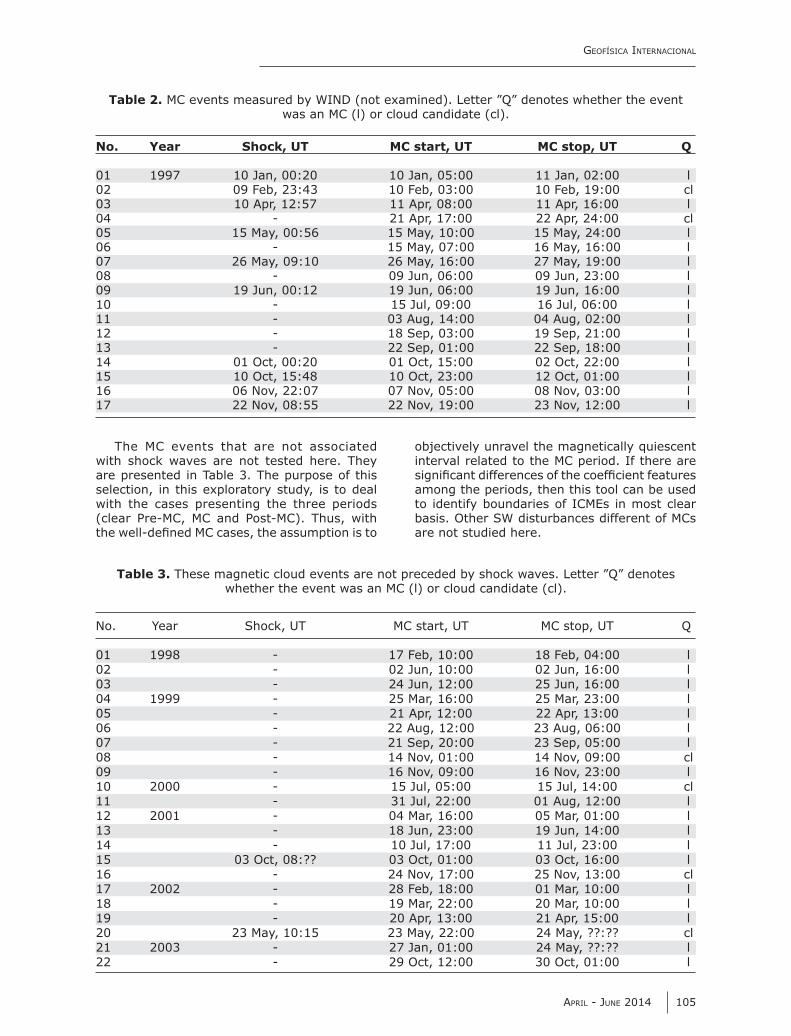
A total of 17 events listed in Table 2 are not treated in this work. The reason is that the

ACE data before about the end of 1997 were et

al. (2005) used the measurements recorded by the WIND spacecraft for this initial period.

-ing dataset from different types of spacecraft. Another problem is that the WIND data avail-able in averages present 3 s, 1 min, and 1 h time resolution, a lower resolution than the one we used by ACE.

Table 1. Solar Wind data studied (from Huttunen et al., 2005).

01 1998 06 Jan, 13:19 07 Jan,03:00 08 Jan, 09:00 10 Jan, 15:0002 03 Feb, 13:09 04 Feb, 05:00 05 Feb, 14:00 06 Feb, 23:0003 04 Mar, 11:03 04 Mar, 15:00 05 Mar, 21:00 07 Mar, 03:0004 01 May, 21:11 02 May, 12:00 03 May, 17:00 04 May, 22:0005 13 Jun, 18:25 14 Jun, 02:00 14 Jun, 24:00 15 Jun, 22:0006 19 Aug, 05:30 20 Aug, 08:00 21 Aug, 18:00 23 Aug, 04:0007 24 Sep, 23:15 25 Sep, 08:00 26 Sep, 12:00 27 Sep, 16:0008 18 Oct, 19:00 19 Oct, 04:00 20 Oct, 06:00 21 Oct, 08:0009 08 Nov, 04:20 08 Nov, 23:00 10 Nov, 01:00 12 Nov, 02:0010 13 Nov, 00:53 13 Nov, 04:00 14 Nov, 06:00 15 Nov, 08:0011 1999 18 Feb, 02:08 18 Feb, 14:00 19 Feb, 11:00 20 Feb, 08:0012 16 Apr, 10:47 16 Apr, 20:00 17 Apr, 18:00 18 Apr, 16:0013 08 Aug, 17:45 09 Aug, 10:00 10 Aug, 14:00 11 Aug, 18:0014 2000 11 Feb, 23:23 12 Feb, 12:00 12 Feb, 24:00 13 Feb, 12:0015 20 Feb, 20:57 21 Feb, 14:00 22 Feb, 12:00 23 Feb, 10:0016 11 Jul, 11:22 11 Jul, 23:00 13 Jul, 02:00 14 Jul, 05:0017 13 Jul, 09:11 13 Jul, 15:00 13 Jul, 24:00 14 Jul, 09:0018 15 Jul, 14:18 15 Jul, 19:00 16 Jul, 12:00 17 Jul, 05:0019 28 Jul, 05:53 28 Jul, 18:00 29 Jul, 10:00 30 Jul, 02:0020 10 Aug, 04:07 10 Aug, 20:00 11 Aug, 08:00 11 Aug, 20:0021 11 Aug, 18:19 12 Aug, 05:00 13 Aug, 02:00 13 Aug, 23:0022 17 Sep, 17:00 17 Sep, 23:00 18 Sep, 14:00 19 Sep, 05:0023 02 Oct, 23:58 03 Oct, 15:00 04 Oct, 14:00 05 Oct, 13:0024 02 Oct, 23:58 13 Oct, 17:00 14 Oct, 13:00 15 Oct, 09:0025 28 Oct, 09:01 28 Oct, 24:00 29 Oct, 23:00 30 Oct, 22:0026 06 Nov, 09:08 06 Nov, 22:00 07 Nov, 15:00 08 Nov, 08:0027 2001 19 Mar, 10:12 19 Mar, 22:00 21 Mar, 23:00 23 Mar, 24:0028 27 Mar, 17:02 27 Mar, 22:00 28 Mar, 05:00 28 Mar, 12:0029 11 Apr, 15:18 12 Apr, 10:00 13 Apr, 06:00 14 Apr, 02:0030 21 Apr, 15:06 21 Apr, 23:00 22 Apr, 24:00 24 Apr, 01:0031 28 Apr, 04:31 28 Apr, 24:00 29 Apr, 13:00 30 Apr, 02:0032 27 May, 14:17 28 May, 11:00 29 May, 06:00 30 May, 01:0033 31 Oct, 12:53 31 Oct, 22:00 02 Nov, 04:00 03 Nov, 10:0034 2002 23 Mar, 10:53 24 Mar, 10:00 25 Mar, 12:00 26 Mar, 14:0035 17 Apr, 10:20 17 Apr, 24:00 19 Apr, 01:00 20 Apr, 02:0036 18 May, 19:44 19 May, 04:00 19 May, 22:00 20 May, 16:0037 01 Aug, 23:10 02 Aug, 06:00 02 Aug, 22:00 03 Aug, 14:0038 30 Sep, 07:55 30 Sep, 23:00 01 Oct, 15:00 02 Oct, 07:0039 2003 20 Mar, 04:20 20 Mar, 13:00 20 Mar, 22:00 21 Mar, 07:0040 17 Aug, 13:41 18 Aug, 06:00 19 Aug, 11:00 20 Aug, 16:0041 20 Nov, 07:27 20 Nov, 11:00 21 Nov, 01:00 22 Nov, 15:00



The MC events that are not associated with shock waves are not tested here. They are presented in Table 3. The purpose of this

with the cases presenting the three periods (clear Pre-MC, MC and Post-MC). Thus, with

objectively unravel the magnetically quiescent interval related to the MC period. If there are

among the periods, then this tool can be used to identify boundaries of ICMEs in most clear basis. Other SW disturbances different of MCs are not studied here.

Table 2.was an MC (l) or cloud candidate (cl).

Table 3. whether the event was an MC (l) or cloud candidate (cl).

01 1997 10 Jan, 00:20 10 Jan, 05:00 11 Jan, 02:00 l02 09 Feb, 23:43 10 Feb, 03:00 10 Feb, 19:00 cl03 10 Apr, 12:57 11 Apr, 08:00 11 Apr, 16:00 l04 - 21 Apr, 17:00 22 Apr, 24:00 cl05 15 May, 00:56 15 May, 10:00 15 May, 24:00 l06 - 15 May, 07:00 16 May, 16:00 l07 26 May, 09:10 26 May, 16:00 27 May, 19:00 l08 - 09 Jun, 06:00 09 Jun, 23:00 l09 19 Jun, 00:12 19 Jun, 06:00 19 Jun, 16:00 l10 - 15 Jul, 09:00 16 Jul, 06:00 l11 - 03 Aug, 14:00 04 Aug, 02:00 l12 - 18 Sep, 03:00 19 Sep, 21:00 l13 - 22 Sep, 01:00 22 Sep, 18:00 l14 01 Oct, 00:20 01 Oct, 15:00 02 Oct, 22:00 l15 10 Oct, 15:48 10 Oct, 23:00 12 Oct, 01:00 l16 06 Nov, 22:07 07 Nov, 05:00 08 Nov, 03:00 l17 22 Nov, 08:55 22 Nov, 19:00 23 Nov, 12:00 l

01 1998 - 17 Feb, 10:00 18 Feb, 04:00 l02 - 02 Jun, 10:00 02 Jun, 16:00 l03 - 24 Jun, 12:00 25 Jun, 16:00 l04 1999 - 25 Mar, 16:00 25 Mar, 23:00 l05 - 21 Apr, 12:00 22 Apr, 13:00 l06 - 22 Aug, 12:00 23 Aug, 06:00 l07 - 21 Sep, 20:00 23 Sep, 05:00 l08 - 14 Nov, 01:00 14 Nov, 09:00 cl09 - 16 Nov, 09:00 16 Nov, 23:00 l10 2000 - 15 Jul, 05:00 15 Jul, 14:00 cl11 - 31 Jul, 22:00 01 Aug, 12:00 l12 2001 - 04 Mar, 16:00 05 Mar, 01:00 l13 - 18 Jun, 23:00 19 Jun, 14:00 l14 - 10 Jul, 17:00 11 Jul, 23:00 l15 03 Oct, 08:?? 03 Oct, 01:00 03 Oct, 16:00 l16 - 24 Nov, 17:00 25 Nov, 13:00 cl17 2002 - 28 Feb, 18:00 01 Mar, 10:00 l18 - 19 Mar, 22:00 20 Mar, 10:00 l19 - 20 Apr, 13:00 21 Apr, 15:00 l20 23 May, 10:15 23 May, 22:00 24 May, ??:?? cl21 2003 - 27 Jan, 01:00 24 May, ??:?? l22 - 29 Oct, 12:00 30 Oct, 01:00 l



The Discrete Wavelet Transform (DWT) is a lin-

popular in data compression (Mallat, 1989; Daubechies, 1992; Hubbard, 1997). Math-ematically, this transform is built based on a multiscale tool called Multiresolution analysis {V j, }∈L2 proposed by S. Mallat (see details in Mallat (1989)), where is a scale function, V j = span{ j

k}, and L2 is the functional space of

the square-integrable functions. The DWT uses discrete values of scale (j) and position (k).

The great contribution of wavelet theory is the characterization of complementary spaces between two embedded spaces V j+1⊂V j, through direct sums V j = V j+1 + W j+1 , where W j = span{ j

k}

with the wavelet function.

simple way to compute this multilevel transform

c jk d j

k associate with

discrete values of scale j and position k. Roughly speaking, the basic ingredients to compute one

h) related to the analysing scale function and its

g) related to

c = h(m k)ckj

mj+2 2 1∑ − (1)

and

d = g(m k)ckj

mj+2 2 1∑ − (2)

The multilevel transform is done by repeating this procedure recursively: convolute the scale

downsampling procedure, i.e., removing one data point between two. Therefore in each scale decomposition levels the number of data is reduced by two. Following is a scheme for the DWT and its inverse (IDWT),

c c ,d ,d ,dj+

IDWT

DWTj j j j j1 1 0{ } ↔ { }− −

.

c j+1.

that their amplitudes are related to the local regularity of the analysed data (Mallat, 1989; Daubechies, 1992). This means that, where

the data has a smooth behaviour, the wavelet

is the basic idea of data compression and the application we are doing here. The wavelet

analysing wavelet order and the scale level.

There is not a perfect wavelet choice for a certain data analysis. However, one can follow certain criteria to provide a good choice, see for instance, Domingues et al. (2005).

In this work, we have chosen the Daubechies scaling function of order 2, with the choice that the wavelet function locally reproduces a linear polynomial. On one hand, high order analysing Daubechies functions are not adding a better local reproduction of the MC disturbance data. On the other hand, the analysing function of order 1 does not reproduce well these disturbances locally.

We have also observed that just one decomposition level is enough for the energy analysis methodology that we propose here, which corresponds to a pseudo-period of 48 s. The pseudoperiod is T

a = (a ) / F

c where a = 2j

is a scale, = 16s is the sampling period, Fc = 0.6667 is the center frequency of a wavelet in Hz (Abry, 1997). In Table 4, as a test, some decomposition levels and the Daubechies scaling function of order 1 to 4 are shown, where F

c =

[0.9961; 0.6667; 0.8000; 0.7143]. Pseudo-periods (seconds) regarding the Daubechies orthogonal wavelets are presented. It also shows that the information here could be

frequencies which is not done in this work.

Table 4. Pseudo-period (seconds) regarding the Daubechies orthogonal wavelets. In this work

=16s, j = 1 and db2 then pseudo-period is 48.0 seconds. The information here could be

frequencies.

Daubechies order 2 analysing wavelet are:

...

j 1 2 3 4

1 32.1 48.0 40.0 44.8 2 64.3 96.0 80.0 89.6 3 128.5 192.0 160.0 179.2 4 257.0 384.0 320.0 358.4 5 514.0 768.0 640.0 716.8



[h0, h

1, h

2, h

3] = 0.4829629131445, 0.8365163037378,

[0.2241438680420, -0.1294095225512] and [g0, g

1,

g2, g

3] = [h

0h

1, h

2h

3] is the high-pass band

In this case, we are using an orthogonal transform. The orthogonal property is very important here, because with it we with it, we can guarantee a preserving energy property in the wavelet transform similarly to the Parseval theorem for Fourier analysis (Daubechies, 1992). Therefore the total energy of the signal is equal to the superposition of the individual contributions of energy of their

(Holschneider, 1991).

In the characterization of a SW disturbance, we perform one decomposition level, and we

d1 or

d1) (energy content on that level), as in Mendes da Costa (2011); Mendes et al. (2005), and its mean value D

d1 is:

D =d

N, N = length f td

ii

N

1 2where

12

1

2

=∑

/

/( ( )) . (3)

This value was calculated in the three regions, for each IMF components (B

x, B

y, B

z). Its values

in the physical system studied. It is lower at a system in stationary state with minimum energy.

then the Dd1

value increases.

form a large-scale winding of a closed magnetic

structure that could be nearly force-free. And it

1 AU (Narock and Lepping, 2007). We do not

An average value ( Dd1

Dd1

calculated:

D = Dd d(i)

i1 1

1

3 =∑

1

3

, (4)

where the angle brackets ... denote an average of the D

d1 in IMF components (i = 1,

2, 3 = Bx, B

y, B

z). Its value is useful to compare

physical point of view, this technique is useful

more perturbations. The Dd1

value increases

for completely random systems.

The treatment procedure is able to characterize regular/non regular behaviour

transition between regions with these two primary behaviours in objective bases. The SW time interval is separated into three new time intervals (windows) corresponding to the preceding sheath or pre-MC, the MC itself, and the SW after the MC or post-MC.

The criterion to select a precise data window after the MC is empirical. Each post-MC region was selected with the same length of the cloud regions. The main effort is to study SW data interval containing the ICMEs, where a shock event and a cloud region were reported. Arbitrary

At the top, IMF Bz (in GSM system) versus time from the ACE spacecraft with 16s time resolution, at

d12

between the vertical dashed lines), and the quiet SW (right of the second vertical dashed line). The lower values of D

d1 are noticed inside of MC region.



selection of post-MC region could affect the results, because this region could be disturbed by other processes unrelated with the MC itself. Thus, the physics of the system should not be changed in the proposed methodology. Further analyses of complicated events can indeed help to understand the true processes occurring in the interplanetary medium. In an evident way, showing the behaviour in the different regions is valuable because only then will be possible

variations (i.e., IMF) could help to separate disturbance processes, e.g., MC-candidate event inside of an ICME. Our hypothesis is that wavelet

leading edge of ICMEs.

We present two case studies based on the analysis of Huttunen et al. (2005), where we have applied this methodology to analyse MC periods (events 14 and 16, Table 1). The study

table, although the results are not presented individually here. In this section, a discussion is done to reach an interpretation.

February 11-13, 2000 ICME event

In Figure 1, at the top, we show the time series of IMF B

z component measured by the

ACE spacecraft at the date February 11; 23:23 UT-February 13; 12:00 UT; 2000. The data was measured in GSM coordinate system with resolution time of 16s. The three regions under

study are separated by two vertical dashed lines. At the bottom, we show the square of the

d1, and results of Dd1. The mean of wavelet

Dd1

in time series at plasma sheath is 0.828 nT2. The result is that the lower D

d1 (0.156

nT2) corresponds to the MC.

In Table 5, the results of Dd1

for the three components of B are presented. Seen in the

always have the lowest Dd1

value. While the higher D

d1 values in all components correspond

to the sheath region.

As a previously known feature, the larger d1, are

indeed associated with abrupt signal locally. From a visual inspection of data, detections may not be an easy task; but the wavelet transforms

Table 5. Mean Dd1

(At top, IMF Bz (in GSM system) versus time from the ACE spacecraft with 16s time resolution, at

d12 vertical dashed lines), and the quiet SW (right of the second vertical dashed line). The high amplitude of d12 inside the third region (Post-MC) is because other event arrived. The lower values of D

d1 is noticed inside of MC region.

Dd1Bx

Dd1By

Dd1Bz

Dd1

Sheath 0.524 0.814 0.828 0.722MC 0.093 0.124 0.156 0.124Post-MC 0.177 0.247 0.319 0.248

Sheath 0.279 0.270 0.625 0.391MC 0.016 0.032 0.042 0.030Post-MC 0.233 0.230 0.458 0.307



July 11-14, 2000 ICME event

In Figure 2, a similar study is done. At the top, we show the time series of IMF B

z component

measured by ACE spacecraft at the date July 11; 11:22 UT-July 14; 05:00 UT; 2000. The three regions under study are separated by two vertical dashed lines. At the bottom, the square

versus time is plotted.

Dd1

in the sheath region is 0.625 nT2. Again the lower D

d1 (0.042 nT2) corresponds to the

MC region; and the higher Dd1

(0.625 nT2) corresponds to the sheath region. The highest amplitude of d12 inside the third region (Post-MC) is due to the arrival of other event (event 17 in Table 1).

Related to this case, the results of Dd1

for the three components of B are presented in

region in the three components always has the lowest D

d1 value. While the highest D

d1 value in

all components correspond to the sheath region.

The tendency of the MC events to have lower values of D

d1 in comparison with the processes

of the other regions. This feature is clearly

be added to the usual features (Burlaga et al., 1981) established earlier for the MCs. Also, we found higher D

d1 values in the sheath. The higher

in the sheath region (see top panel on Figures 1 and 2).

41 ICMEs events

Aiming to a conclusive analysis, the calculations D

d1 for the three IMF components are done for

the other cases of Table 1. The procedure is identical to the one used in the previous studies.

In Figure 3, the Dd1

values versus number of events were plotted respectively as squares, cross-circles symbols, and triangles symbols, correspond respectively to the sheath, MC and Post-MC regions. We can compare the D

d1values of the three regions for every event. The D

d1values are higher in the sheath region in

35/41 or 85.4% events. This does not occur in the events numbered as 4; 5; 6; 13; 24; 34 in Table 1, where the highest values are found in

Post-MCs as shown in Figure 2, there may be an arrival of a shock or an ICMEs. However, the

greater than one in the cloud that follows. In particular, the magnetic field fluctuation in some MC regions (events numbered as 9; 19; 17; 20; 21; 31; 41) is greater than one in the

are not low in all MCs, in some cases waves can penetrate from the sheath to the cloud. In this paper, the goal is to test the usefulness of

physical process.

. The Dd1

values versus number of events were plotted respectively as squares, cross circles symbols,

scale, because is best to visualization.



Figure 4 shows a histogram constructed from the occurrence frequencies of the D

d1values. The D

d1values for the sheath, MC

and Post-MC regions are plotted respectively

sets of bars on the left, while there are 4.9% and 24.4% of the sheaths and Post-MC regions

some sheath regions. This means that if an ICME is not moving faster than the surrounding SW (Klein and Burlaga, 1982; Zhang and Burlaga, 1988; Burlaga, 1988), the sheath region does not present a very corrugated feature in the

be done under these conditions. Conversely, in the last four sets of bars we have 75.6% of the sheaths and only 12.2% of the MCs regions. The results presented in the two previous case

sheath, and the lowest ones are during the D

d1values to identify the three different regions. Figure 4 only allows the comparison between values from the three regions in the same event. We can conclude that there is not a

Figure 4 shows that due to the overlapping observed between the three distributions, this technique could not be used to identify boundaries automatically. It provides an objective analysis technique that helps in

of ICME, fundamentally the cloud boundaries. This technique could be useful to help a

IMF dataset.

As in Table 5, the higher Dd1 values are found

in Bz component for every region. By direct visual

inspection, most of the time, this detection is not possible. However, the wavelet transform

Bz

component is very important in the magnetic reconnection at Earth’s magnetopause. An open question could be asked: how important are the

of this technique in order to evaluate the SW

help to obtain a better visualization of the shock and to identify the initial border of the MC.

behaviours of the physical processes underlying in the magnetic records. This is understandable, because the MC has a geometric structure in

and the “quiet” SW. The sheath is naturally a

in the IMF data with large Dd1 values. A smoother

Dd1

or an increasing of random characteristics, or even turbulences from an arrival event (for the latter, e.g., the events 16 and 20). Sometimes, the Post-MC region has a large D

d1 value due

If this technique is applied to a large dataset

also large in other regions in which there are no ICMEs. On other hand, the wavelet

regions. Although it does not allow identifying

A histogram is constructed from a frequency table of D

d1values; the

by 0.01. The Dd1

values for the sheath, MC and post MC, the three select regions, plotted as the grey, black

and white.



clouds automatically, it is an useful tool for

(MVA) is used. In fact, we have used for this purpose. In our opinion, the presentation of this tool for the Space Physics Community could “open doors” for other applications. For

SW with different pseudo-frequencies can be investigated.

Application to identify the shock and leader edge of ICME

The formation of a sheath implied in the

if the MC is moving at the same speed as the

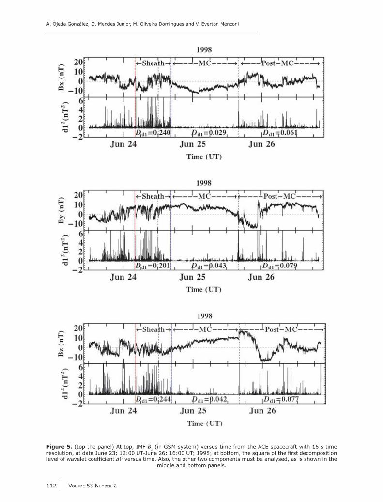
both the SW ahead and behind, creating sheath-like structures (though they may not be bounded by a shock front). This study considers the events of MCs not associated with evident shock waves, presented in Table 3 (see event 3). With illustrative purpose, a case study is presented for the date June 24; 12:00 UT-June 25; 16:00 UT; 1998. The criteria to select the data interval after the MC are the same used previously. The duration time in regions at 41 sheaths is less than one day, and then a region with this equivalent duration from the initial time of the cloud is chosen.

In Figure 5, the above interval at the date June 23; 12:00 UT-June 26; 16:00 UT; 1998 is shown. Each panel presents respectively, from top to bottom, B

x, B

y and B

z time series

respectively. At the bottom of the respective

is plotted. The two vertical dashed lines correspond to the MC region delimitations identified by Huttunen et al. (2005). The

observed inside the initial border of MC, then we

So, the leader edge at date June 24; 16:32 UT

corresponds to the previous data.

identify sheath like structures. However, the

discontinuity implies the use of plasma data. So, a probable discontinuity at date June 24; 04:00

of SW plasma parameters, an interplanetary

sheath-like structure can be associated to this

to the start of its location.

In Figure 5 (all panels), the Dd1

values in each regions are shown. We found higher D

d1

values in the sheath-like structures while the lower values correspond to cloud region. The results related to this part are consistent with the earlier results.

In conclusion, this methodology has a practical application. Maybe other applications for Space Physics Community uses will be found,

occur in several frequency ranges.

We deal with time series of SW for a group of magnetic clouds in order to analyse the

Bx, B

y and B

z components.

The mathematical property chosen here was the D

d1)

which was obtained by applying the discrete orthogonal wavelet transform using Daubechies wavelet of order two (i.e. Daubechies scale

IMF as recorded by the instruments of the MAG on-board of the ACE S/C at the L1 point.

The main point in the use of the amplitude of

represent the local regularity present in the signal in study (Mallat, 1989). They were constructed

between a certain local polynomial reproduction and the signal itself. This is used to identify local regularity in high order derivatives in the analysed signal. The local regularity changes can be therefore highlighted by means of the

even possible to see discontinuities in high order derivatives that cause disturbances by visual inspection of the signal. For instance, using Daubechies wavelet of order 2, discontinuities

and measured, respectively. We use that

highlight possible regions of regularity on the

an ICME event measure at IMF datasets. The results show that there is, apparently, a clear distinction between the values of the wavelet

of the passing magnetic structure (ahead of the MC, i.e., the sheath; the MC itself; and after the passage of the MC (Post-MC)). The measurements show that D

d1values during the passage of the MC. Also, we found higher values in the sheaths.



(top the panel) At top, IMF Bx (in GSM system) versus time from the ACE spacecraft with 16 s time

d12 versus time. Also, the other two components must be analysed, as is shown in the

middle and bottom panels.



Using assumptions that concern the physics of MC, the analyses developed in this work

main reason of the lower values of wavelet coefficients during it. This study has been

of which were structures that appeared to be MCs. This tool allows for the comparison of the

Bx, B

y and B

z, which it is not an easy task under

simple visual inspection. The Bx component has

Bz

component the higher ones.

We can identify the effect of shock waves in the change of the local regularity of the IMF component using its d12 time series, shows

decreases at transient regions in MC boundaries -

of entropy and variance respectively, and then

them. The previous behaviour is not true for all the cases because some another phenomenon could also be present. However, in this study

all magnetic clouds, in some cases waves can penetrate from the sheath to the cloud. The

This is an objective analysis technique pro-

-sitions in the IMF regularity for different regions

regions. It can be very useful for specialists, -

that are not easy to be seen in the IMF data by simple visual inspection.

By now, only assumptions for proper MCs were validated. Maybe this methodology could

CIR, heliospheric current sheath crossings or ICMEs without MC signatures which has not yet been done.. Such an approach aiming at new facilities for the Space Physics community efforts seem to be an important contribution.

This work was supported by grants from CNPq (grants 483226 /2011-4, 307511 /2010-3, 306828 /2010-3 and 486165 /2006-0), FAPESP (grants 2012 /072812-2, and 2007 /07723-7) and CAPES (grants 1236-83 /2012 and 86 /2010-29). A.O.G. thanks the CAPES and CNPq (grant 141549/2010-6) for his PhD scholarship and CNPq (grant 150595/2013-1) for his postdoctoral research support. V. E. Menconi thanks to the grants FAPESP 2008/09736-1, CNPq 3124862012-0 and 455097/2013-5. We also wish to thank the anonymous referees for improvement of this paper.

The local regularity changes can be therefore highlighted by means of the amplitude wavelet coefficients. Using the signal presented in (Daubechies, 1992, p.301), we constructed the

Considering,

f x

e if x

e if x

e x if x

x

x

x

( )

,

[( ) ]

| |

| |=

≤−

− < ≤

− +

−

−

−

2 1

1 1

1 12 ≥≥

⎧

⎨

⎪⎪⎪⎪⎪⎪⎪

⎩

⎪⎪⎪⎪⎪⎪⎪1;

,

x = -1at that point and in the point x = 0 and the second derivative is discontinuous at these

At top, the signal f(x)± (x(x) is a white noise. At the bottom,

d12 (x)/10-12



points. We compute one decomposition level of discrete orthogonal wavelet transform using a Daubechies wavelet of order 2. The result is presented in the Figure A.6, the larger amplitude

points where the signal has changes in the local regularity.

Abry P., 1997, Multirésolutions, algorithmes de décomposition, invariance d’échelles, diderot Edition. Ondelettes et turbulence. Paris.

Borovsky, J.E., 2012, The velocity and magnetic

Statistical analysis of Fourier spectra and correlations with plasma properties. Journal of Geophysical Research, 117, A5.

Bothmer, V., Schwenn, R., 1998, The structure and origin of magnetic clouds in the solar wind. Annales Geophysicae 16, 1–24,

Burlaga, L., 1988, Magnetic clouds and force-ournal of

Geophysical Research, 93, 7217.

Burlaga, L., Behannon K., 1982, Magnetic clouds: Voyager observations between 2 and 4 AU. Solar Physics, 81, 181.

Burlaga L.F., 1995, Interplanetary Magnetohy-

Burlaga, L. F., Sittler, E., Mariani, F., Schwenn, R., 1981, Magnetic loop behind an interplanetary shock: Voyager, Helios and IMP 8 observations. Journal of Geophysical Research, 86, 6673–6684.

Celletti A., Giorgilli A., 1990, On the stability of the lagrangian points in the spatial restricted problem of three bodies. Celestial Mechanics and Dynamical Astronomy, 50, 1, 31–58.

Dal Lago A., Gonzalez W., Gonzalez A.,

plasma parameters for magnetic clouds in the interplanetary medium. Geofísica Internacional, 39, 1, 139–142.

Dal Lago A., Gonzalez W.D., Gonzalez A., Vieira L.E.A., 2001, Compression of magnetic clouds in interplanetary space and increase in their geoeffectiveness. Journal of Atmospheric and Solar-Terrestrial Physics, 63, 451–455.

Dasso S., Mandrini C., Démoulin P., Luoni M., Gulisano A., 2005, Large scale MHD properties of interplanetary magnetic clouds. Advances in Space Research, 35, 711–724.

Daubechies I., 1992, Ten lectures on wavelets. Society for Industrial and Applied Mathematics, Philadelphia, PA, USA.

Démoulin P., Dasso S., 2009, Causes and

Astronomy and Astrophysics, 498, 2, 551–566.

Domingues M.O., Mendes O., Mendes da Costa A., 2005, Wavelet techniques in atmospheric sciences. Advances in Space Research, 35 5, 831– 842.

Echer E., Alves M., Gonzalez W., 2005, A statistical study of magnetic cloud parameters and geoeffectiveness. Journal of Atmospheric and Solar- Terrestrial Physics 67, 10, 839–852.

Farrugia C.J., Osherovich V.A., Burlaga L., 1995,

as Models for Interplanetary Magnetic Clouds. Journal of Geophysical Research, 100, A7, 12293–12306.

Gonzalez W.D., Tsurutani B.T., 1987, Criteria of interplanetary parameters causing intense magnetic storms (Dst<-100nT). Planetary and Space Science, 35, 9, 1101–1109.

Gosling J., 1990, Coronal mass ejections and

In: Russel, C. T., Priest, E. R., Lee, L. C.

Geophys. Monogr., p. 343.

ejections at high heliographic latitudes: Observations and simulations. Journal of Geophysical Research, 103, A2, 1941–1954.

Holschneider M., 1991, Inverse Radon transforms through inverse wavelet transforms. Inverse Problems 7, 6, 853.

Hubbard B.B., 1997, The World According to Wavelets: The Story of a Mathematical Technique in the Making. A K Peters Ltd.

Huttunen K.E.J., Schwenn R., Bothmer V., Koskinen H.E.J., 2005, Properties and geoeffectiveness of magnetic clouds in the

of solar cycle 23. Annales Geophysicae, 23, 625– 641.



Kim H.-J., Lyons L., Boudouridis A., Lee D.-Y., Heinselman C., Mc-Cready M., 2009,

substantially affect the strength of dayside ionospheric convection. Journal of Geophysical Research, 114, A11305, 14.

Klein L.W., Burlaga L.F., 1982, Interplanetary magnetic clouds at 1 AU. Journal of Geophysical Research, 87, 613–624.

Lepping, R., Burlaga, L., Szabo, A., Ogilvie, K., Mish, W., 1997. The Wind magnetic cloud and events October 18-20, 1995: interplanetary properties and as triggers for geomagnetic activity. Journal of Geophysical Research, 102, A7, 14, 049–14,063.

Lepping R.P., Berdichevsky D., Pandalai S.G., 2000, Interplanetary magnetic clouds: Sources, properties, modeling, and geomagnetic relationship. Recent research developments in geophysics, 77–96 Eng.

Lepping R.P., Jones J.A., Burlaga L.F., 1990, Interplanetary magnetic clouds at 1 AU. Journal of Geophysical Research, 95, 11957.

Ark Fys, 2, 361–365.

Lyons L., Kim H.-J., Xing X., Zou S., Lee D.-Y., Heinselman C., Nicolls M., Angelopoulos V., Larson D., McFadden J., Runov A., Fornacon K.- H., 2009, Evidence that solar

convection and substorm occurrence. Journal of Geophysical Research, A11306, 14.

mations and wavelet orthonormal bases of L2, R, 315, 1, 69–87.

Mendes O.J., Domingues M.O., Mendes da Costa A., 2005, Wavelet analysis applied to magnetograms. Journal of Atmospheric and Solar-Terrestrial Physics, 67, 1827–1836.

Mendes da Costa A., Oliveira Domingues M., Mendes O., Marques B., Christiano G., 2011, Interplanetary medium condition effects in the south Atlantic magnetic anomaly: A case study. Journal of Atmospheric and Solar-Terrestrial Physics, 73, 11-12, 1478–1491.

Narock T.W., Lepping R.P., 2007, Anisotropy of

interplanetary magnetic cloud at 1 AU. Journal of Geophysical Research, 112, A06108, 6.

Ojeda G.A., Calzadilla M.A., Lazo B., Alazo K., Savio O., 2005, Analysis of behavior of solar wind parameters under different IMF conditions using nonlinear dynamics techniques. Journal of Atmospheric and Solar- Terrestrial Physics, 67, 17-18, 1859–1864.

Ojeda G.A., Mendes O., Calzadilla M.A., Domingues M.O., 2013, Spatio-temporal

help magnetic cloud characterization, J. Geophys. Res. Space Physics, 118, 5403-5414, doi:10.1002/jgra.50504.

Osherovich V., Burlaga L.F., 1997, Magnetic Clouds. In: Crooker, N., Joselyn, J., Feynman, J. (Eds.), Coronal Mass Ejection. Vol. 99. AGU,Washington, D. C., p. 157.

Siscoe G., Odstrcil D., 2008, Ways in which ICME sheaths differ from magnetosheaths. Journal of Geophysical Research, 113 A00B07, 1–10.

M.H., Burlaga L.F., Scheifele J., 1998, The Space

Science, 86, 613–632.

Tsurutani B.T., Gonzalez W.D., 1992, Great magnetic storms. Geophysical Research Letters, 19, 1, 73–76.

Tsurutani B.T., Gonzalez W.D., Tang F., Akasofu S.I., Smith E.J., 1988, Origin of Interplanetary Southward Magnetic Fields Responsible for Major Magnetic Storms

Journal of Geophysical Research, 93, 8519–8531.

Wu C.-C., Lepping R.P., 2002a, Effect of solar wind velocity on magnetic cloud-associated magnetic storm intensity. Journal of Geophysical Research, 107, A11, 1346–1350.

Wu C.-C., Lepping R.P., 2002b, Effects of magnetic clouds on the occurrence of geo-

Journal of Geophysical Research, 107 A10, 1314–1322.

Zhang G., Burlaga L.F., 1988, Magnetic clouds, geomagnetic disturbances and cosmic ray decreases. Journal of Geophysical Research, 88, 2511.

Documents

Daubechies wavelet coefficients: a tool to study ... · GEOFÍSICA INTERNACIONAL APRIL - JUNE 2014 103 ÀXFWXDWLRQV DUH DQ LPSRUWDQW FRQWULEXWRU WR the large-scale transfer of SW