Embed Size (px)
Citation preview

Copyright
by
David Alexander Robbins Debeau
2019
The Dissertation Committee for David Alexander Robbins Debeau Certifies that
this is the approved version of the following Dissertation:
2.5D AND CONFORMAL NEGATIVE STIFFNESS HONEYCOMBS
UNDER STATIC AND DYNAMIC LOADING
Committee:
Carolyn C. Seepersad, Supervisor
Michael R. Haberman
Desiderio Kovar
Allen Roach
2.5D AND CONFORMAL NEGATIVE STIFFNESS HONEYCOMBS
UNDER STATIC AND DYNAMIC LOADING
by
David Alexander Robbins Debeau
Dissertation
Presented to the Faculty of the Graduate School of
The University of Texas at Austin
in Partial Fulfillment
of the Requirements
for the Degree of
Doctor of Philosophy
The University of Texas at Austin
May 2019

Dedication
To my loving girlfriend Erin.
v
Acknowledgements
I would like to thank Dr. Seepersad for introducing me to negative stiffness
honeycombs and allowing me to join her lab in 2015. Her support has made graduate
research a rewarding and relatively painless experience. I have learned a significant
amount about teaching and mentoring from her, in addition to technical topics.
I would like to thank Clint Morris, Jared Allison, Conner Sharpe, Oliver Uitz,
Tyler Wiest and Ademola Oridate for their support along the way. Conducting research in
a lab with such talented individuals has greatly helped my work and raised my standards.
Thank you for answering questions and being there to bounce ideas off of.
Undergraduate researchers Zahra Ahmed and Max Garufo were a significant help
with conducting experiments and building test equipment. Working with them reduced
my work load significantly.
This research was sponsored by an LDRD from Sandia National Laboratories.
Without sponsorship it would have taken much longer to complete the research. Dynamic
impulse testing would have been difficult to conduct and results would have taken longer
to analyze. This project would not have been possible without Tommy Woodall, Nicholas
Leathe, Audrey Morris-Eckart, Allen Roach, Andrew Lentfer, Matthew Spletzer and
Peter Renslow.
Vulcan Labs was instrumental in providing high quality conformal negative
stiffness prototypes. Without them it would have cost thousands of dollars and taken
months to manufacture prototypes. I would like to thank Ben Fulcher and David Leigh
for their engineering expertise and support.
vi
Abstract
2.5D and Conformal Negative Stiffness Honeycombs under Static and
Dynamic Loading
David Alexander Robbins Debeau, Ph.D.
The University of Texas at Austin, 2019
Supervisor: Carolyn C. Seepersad
Negative stiffness honeycombs have been shown to provide nearly ideal impact
mitigation with elastically recoverable configuration and mechanical behavior. This
capability allows for reliable mitigation of multiple impacts, which conventional
honeycombs cannot accommodate because of plastic deformation and collapse. A more
in-depth characterization of the mechanical behavior of these negative stiffness
honeycombs is presented. The starting point is a 2.5D configuration in which the negative
stiffness honeycomb configuration is varied in-plane and extruded out-of-plane. Impact
mitigation is investigated by subjecting the 2.5D honeycombs to various drop heights on
a purpose-built, drop-test rig. Several embodiments of the 2.5D honeycomb are designed
and tested, including nylon versus aluminum, constrained versus unconstrained, and
altered configurations with different numbers of rows and columns of negative stiffness
elements.
While the 2.5D configuration performs well in response to in-plane loading, it is
not designed to accommodate out-of-plane loading. A conformal negative stiffness
honeycomb design is introduced that conforms to curved surfaces and accommodates
vii
out-of-plane loading that is not orthogonal to the load concentrator on top of the
honeycomb. Quasi-static mechanical and dynamic mechanical impulse testing of the
conformal honeycomb are conducted to characterize the mechanical performance of the
conformal design. The final chapter includes a multi-element study that demonstrates
how multiple elements perform in an assembly in a more realistic setting.
A FEA framework is built to automate the simulation of the 2.5D and conformal
negative stiffness honeycomb designs. The framework is built within the commercial
Abaqus® FEA package using its Python scripting interface. Automating the design,
meshing, loading, and boundary conditions allows for rapid design iteration. Simulations
using the FEA framework are compared to experimental quasi-static, impact, and impulse
tests.
The conformal design was developed to be manufactured additively. The additive
manufacturing process introduces sources of potentially significant geometric and
material property variability that affect the performance of the honeycombs. The FEA
framework is used to conduct a predictability and reliability study that incorporates
several sources of variability into the analysis and returns estimates of the expected force
threshold and its distribution.
viii
Table of Contents
List of Tables ................................................................................................................... xiii
List of Figures .................................................................................................................. xiv
Introduction to Negative Stiffness Honeycombs ...............................................1
1.1: Negative Stiffness Honeycomb Design ...............................................................3
1.2: Research Goals ..................................................................................................10
Goal 1: Design a conformal negative stiffness element that protects
objects with curved surfaces. ..................................................................10
Goal 2: Conduct quasi-static and dynamic FEA of the 2.5D and
conformal designs to predict quasi-static and impact performance. .......10
Goal 3: Conduct quasi-static and dynamic testing of 2.5D and
conformal negative stiffness designs to evaluate impact performance...11
Goal 4: Conduct dynamic impulse testing at Sandia National
Laboratories to evaluate the performance of conformal negative
stiffness honeycombs under high acceleration impulses. .......................11
Goal 5: Model the manufacturing-induced variability in the conformal
negative stiffness honeycombs to evaluate the predictability and
reliability of their impact performance. ..................................................12
Goal 6: Conduct multi-element testing to evaluate performance under
more realistic conditions. ........................................................................12
1.3: Chapter Summary ..............................................................................................12
Chapter 2: Methods of Analysis ..................................................................12
Chapter 3: 2.5D Negative Stiffness Honeycomb Experiments ....................13
Chapter 4: Conformal Negative Stiffness Honeycomb Experiments ..........13
Chapter 5: Predictability and Reliability Modeling .....................................13
Chapter 6: Multi-Element Assembly ...........................................................14
ix
Chapter 7: Conclusion .................................................................................14
Analysis of Quasi-static and Dynamic Behavior of Negative Stiffness
Honeycombs ................................................................................................................15
2.1: Negative Stiffness Honeycomb Designs ...........................................................15
2.5D Negative Stiffness Honeycomb............................................................15
Conformal Negative Stiffness Honeycomb ..................................................16
2.2: Analytical Method .............................................................................................18
2.3: Parametric FEA Model ......................................................................................22
2.4: Quasi-static FEA ................................................................................................25
2.5: Dynamic FEA ....................................................................................................28
Impact Analysis ............................................................................................28
Impulse Analysis...........................................................................................30
2.6: Simulating Multiple Compressions ...................................................................34
2.5D Negative Stiffness Honeycomb Experiments ..........................................37
3.1: Manufacture of 2.5D Design .............................................................................38
Thermoplastic Prototypes .............................................................................38
Aluminum Prototypes ...................................................................................39
3.2: Design Considerations .......................................................................................40
3.3: Quasi-static Compression Testing of 2.5D Honeycombs ..................................42
Metal Prototype.............................................................................................42
Thermoplastic Prototype ...............................................................................44
3.4: Dynamic Impact Testing of 2.5D Honeycombs ................................................45
Metal Prototype Impact Testing ...................................................................47
Thermoplastic Prototype ...............................................................................52
x
3.5: Conclusion .........................................................................................................57
Conformal Negative Stiffness Honeycomb Experiments ................................58
4.1: Design and Manufacture of Thermoplastic Conformal Negative Stiffness
Elements..............................................................................................................59
Thermoplastic Design ...................................................................................60
4.2: Design and Manufacture of Metal Conformal Negative Stiffness Elements ....62
Metal Design .................................................................................................65
4.3: Quasi-static Compression Testing of Conformal Honeycomb Prototypes ........68
Thermoplastic Prototypes .............................................................................68
Metal Prototypes ...........................................................................................70
4.4: Dynamic Impulse Testing of Metal Conformal Prototypes ...............................74
4.5: Conclusion .........................................................................................................79
Predictability and Reliability Modeling ...........................................................81
5.1 Predictability of Mechanical Behavior of Direct Metal Laser Sintered Parts ....81
5.2 Material Property Testing ...................................................................................85
5.3 Modeling Variability in Mechanical Performance .............................................89
Material Properties ........................................................................................89
Beam Thickness, Beam Height, and Shape Imperfections ...........................93
5.4 Uncertainty Analysis.........................................................................................112
5.5 Uncertainty Analysis Results ............................................................................113
Design and Impulse Testing of a Multi-Element Assembly ..........................123
6.1 Multi-Element Design.......................................................................................123
Multi-Element Base Design ........................................................................123
Element Design ...........................................................................................127
xi
6.2 Quasi-Static Testing of Multi-Element Assemblies .........................................130
Test Setup ...................................................................................................130
Results .........................................................................................................131
Simulation ...................................................................................................135
6.3 Multi-Element Impulse Testing Fixture ...........................................................138
6.4 Dynamic Impulse Testing of Multi-Element Assemblies.................................140
Results .........................................................................................................141
Simulation ...................................................................................................147
Conclusion ..................................................................................................150
Conclusion......................................................................................................151
7.1: Research Contributions ....................................................................................151
A conformal negative stiffness element was designed to protect objects
with curved surfaces. ............................................................................151
Quasi-static and dynamic FEA of the two dimensional and conformal
elements was conducted to predict their impact mitigation
performance. .........................................................................................152
Quasi-static and dynamic testing of 2.5D and conformal negative
stiffness elements was conducted to evaluate their impact mitigation
performance and compare it with simulation-based predictions. .........153
Dynamic impulse testing at Sandia National Laboratories was conducted
to investigate the impact mitigation performance of conformal
negative stiffness elements under extremely high acceleration
impulses. ...............................................................................................154
A predictability and reliability study was conducted to evaluate the
effect of various sources of uncertainty or variability on the impact
mitigation performance of conformal elements. ...................................155
Multi-element testing was conducted to evaluate the impact mitigation
performance of conformal elements under more realistic conditions...156
xii
7.2: Future Work .....................................................................................................157
Fatigue Testing ...........................................................................................157
Investigate Build Orientation ......................................................................157
Adding Damping Material ..........................................................................157
Metal Conformal Design Energy Dissipation .............................................158
Negative Stiffness Designs for Helmets .....................................................158
References ........................................................................................................................159
xiii
List of Tables
Table 3.1: Table of as-built properties of the nylon and aluminum prototypes. Figure
3.1 shows the labels used to represent the beam. ..........................................41
Table 4.1: Table of as-designed properties for nylon conformal honeycombs ..................62
Table 4.2: Material properties for H1150 17-4 PH stainless steel .....................................66
Table 4.3: Table of as-designed properties for metal design .............................................68
Table 4.4: Comparison of different analysis methods to experimental results ..................70
Table 5.1: Material properties for Vulcan maraging steel tensile bars ..............................88
Table 5.2: Material properties reported by Renishaw [41] ................................................89
Table 5.3: Weibull Distribution Parameters for the original Sandia National
Laboratories study and the modified values .................................................90
Table 5.4: As-designed dimensions and standard deviations for uncertainty analysis ....113
Table 5.5: Statistics for the results in Figure 5.33 and Figure 5.34 .................................119
Table 5.6: Force threshold taken as the maximum force for the first snap through
event. Mean: 275 N, Stdev: 2.43 N .............................................................120
Table 6.1: Table of base designs used in the multi-element study ..................................126
Table 6.2: Table of as-designed properties for multi-element design .............................128
Table 6.3: Peak acceleration for a 10,000 G, 0.1 ms impulse. Responses were filtered
using a 5 kHz cut off frequency. .................................................................146
xiv
List of Figures
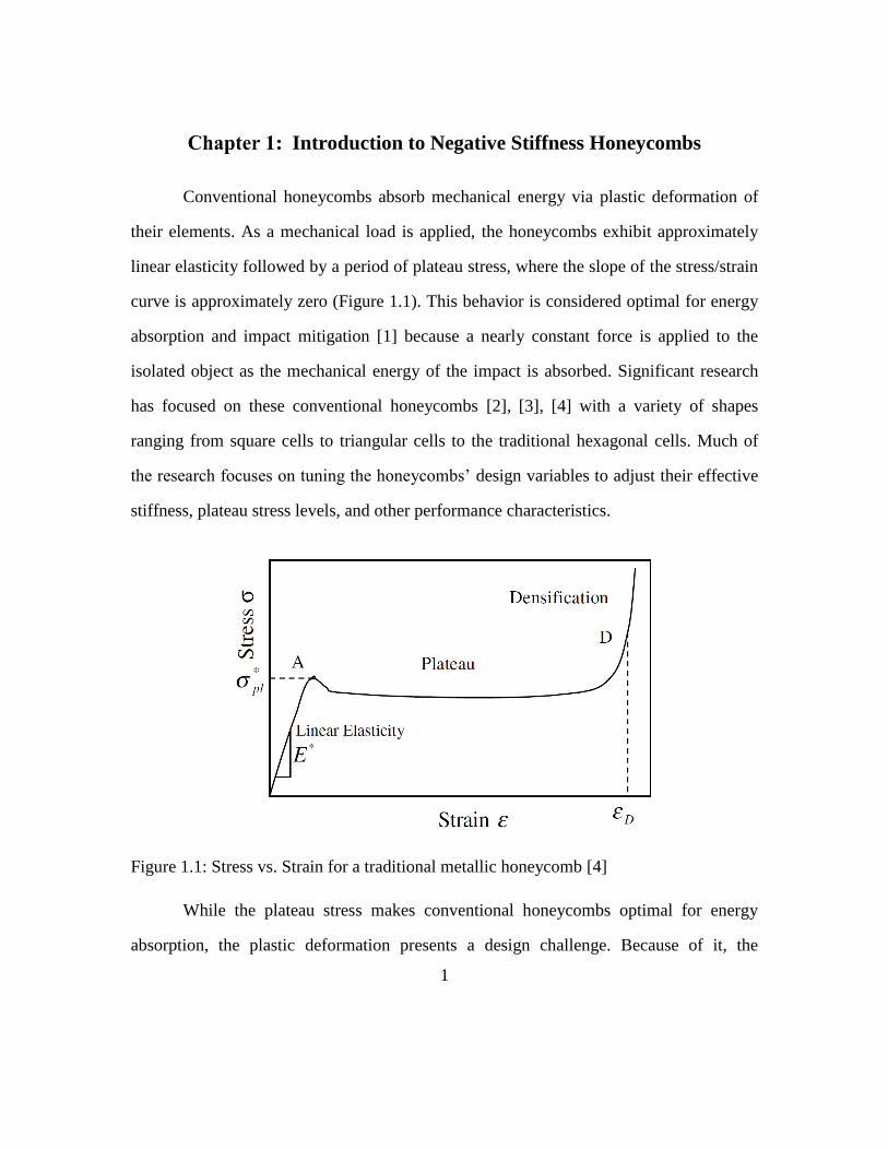
Figure 1.1: Stress vs. Strain for a traditional metallic honeycomb [4] ................................1
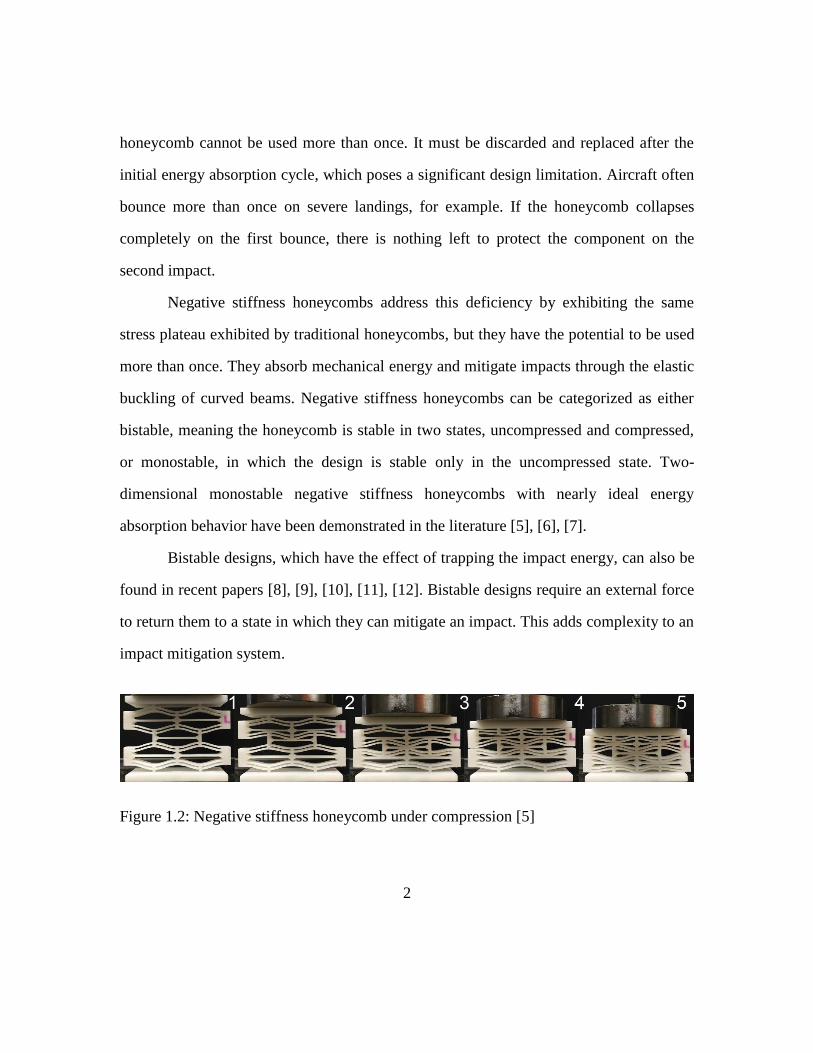
Figure 1.2: Negative stiffness honeycomb under compression [5]......................................2
Figure 1.3: Negative stiffness beam [6] ...............................................................................4
Figure 1.4: Buckling mode shapes for a beam with clamped ends [17] ..............................4
Figure 1.5: Force displacement curve [5] ............................................................................5
Figure 1.6: Aluminum 2.5D negative stiffness honeycomb ................................................7
Figure 1.7: Quasi-static compression of aluminum 2.5D negative stiffness
honeycomb. Hysteresis is nearly absent from the load-unload plot. ..............7
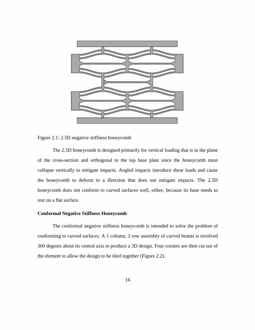
Figure 2.1: 2.5D negative stiffness honeycomb .................................................................16
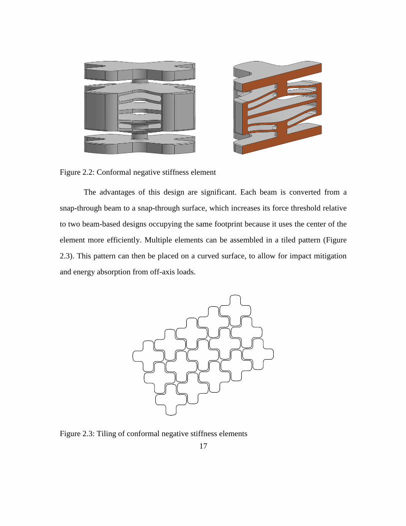
Figure 2.2: Conformal negative stiffness element .............................................................17
Figure 2.3: Tiling of conformal negative stiffness elements .............................................17
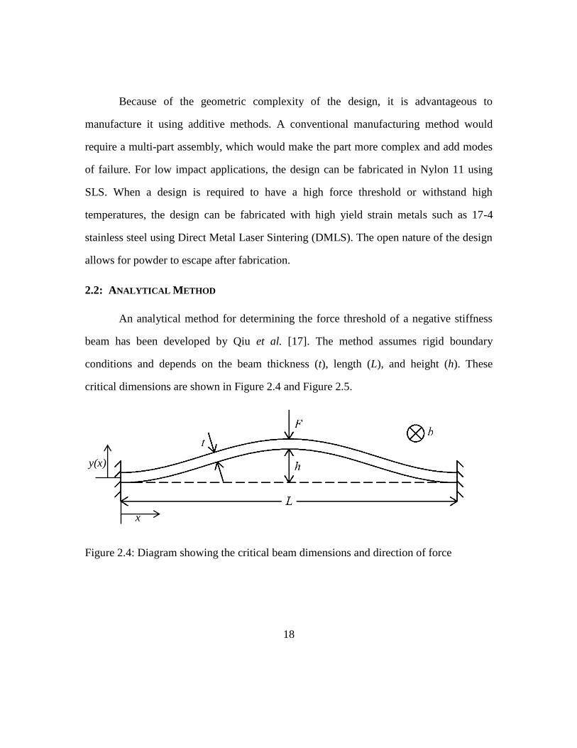
Figure 2.4: Diagram showing the critical beam dimensions and direction of force ..........18
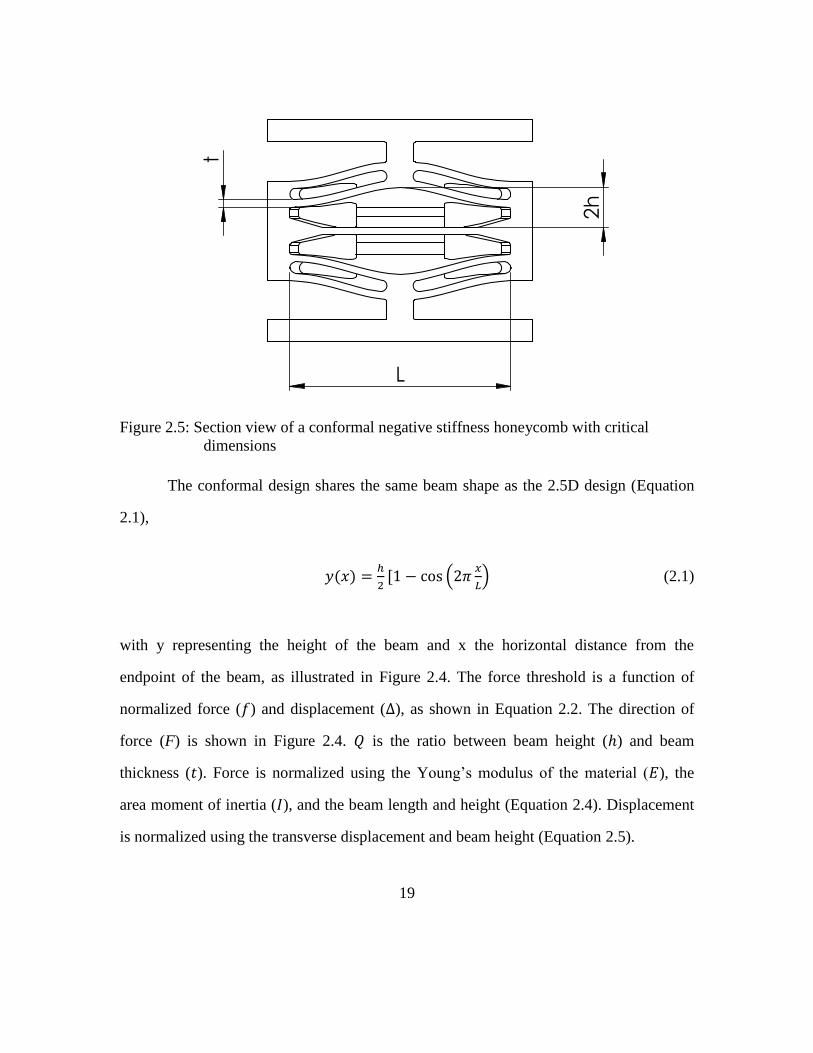
Figure 2.5: Section view of a conformal negative stiffness honeycomb with critical
dimensions ....................................................................................................19
Figure 2.6: Normalized force (f) versus normalized displacement (∆) [17] ......................20
Figure 2.7: Top view of conformal negative stiffness design that shows how the
design can be approximated by two 2.5D designs ........................................22
Figure 2.8: Shell/Solid hybrid model of conformal design................................................25
Figure 2.9: Boundary conditions for FEA of conformal design ........................................27
Figure 2.10: Comparison of explicit quasi-static method to modified-Riks method .........28
Figure 2.11: Diagram of dynamic impact type analysis ....................................................29
Figure 2.12: Example of a 15,000 G impulse over 1.0 ms ................................................31
Figure 2.13: Velocity profile for a 15,000 G impulse over 1.0 ms ....................................32
xv
Figure 2.14: Diagram of dynamic impulse type analysis ..................................................33
Figure 2.15: Example acceleration output from dynamic impulse simulation ..................34
Figure 2.16: Steps of multiple compression analysis ........................................................35
Figure 2.17: Multi-step Riks analysis allows for more accurate force threshold
determination ................................................................................................36
Figure 3.1: Depth of 2.5D design is designated by (b) ......................................................37
Figure 3.2: Negative Stiffness Honeycomb under Compression [5] .................................37
Figure 3.3: Build Platform Orientation [28] ......................................................................39
Figure 3.4: Aluminum 2.5D honeycomb showing the 80/20 angle brackets used to
support the design .........................................................................................40
Figure 3.5: Quasi-static force vs. displacement plot for 2.5D aluminum prototype ..........43
Figure 3.6: Quasi-static force vs. displacement plot for 2.5D nylon prototype .................45
Figure 3.7: Custom build drop-test rig with 80/20 frame (A), steel base plate (B), 5 kg
impact plate (C), cantilever 80/20 arm (D), accelerometer (F), vertical
80/20 rail (E), and velocity meter (G) ...........................................................46
Figure 3.8: 1 V signal over time showing the contact of the drop rig bolt with the
velocity meter pencil leads............................................................................47
Figure 3.9: Metal 2.5D design shown in uncompressed (monostable) and compressed
configuration. Twelve zip ties are used to keep the design in the
compressed configuration. ............................................................................48
Figure 3.10: Dynamic impact of 5.0 kg plate from a 12.7 cm drop height onto a metal
2.5D honeycomb in compressed and uncompressed configurations with
time scale limited to a single bounce of the plate .........................................49
xvi
Figure 3.11: Dynamic impact of 5.0 kg plate from a 12.7 cm drop height onto a metal
2.5D honeycomb in compressed and uncompressed configurations with
time scale lengthened to show multiple bounces until the plate comes to
rest .................................................................................................................50
Figure 3.12: Diagram of wedge cut made by water jet machine .......................................51
Figure 3.13: Dynamic impact response of 2.5D metal honeycomb compared to
simulation results using the as-designed beam thickness of 1.00 mm and
the average as-built beam thickness of 1.13 mm. .........................................52
Figure 3.14: Dynamic impact of 5.0 kg plate from a drop height of 12.7 cm onto a
nylon 2.5D honeycomb in compressed and uncompressed configurations
with time scale shortened to represent only the first bounce of the impact
plate ...............................................................................................................53
Figure 3.15: Dynamic impact of 5.0 kg plate from a drop height of 12.7 cm onto a
nylon 2.5D honeycomb in compressed and uncompressed configurations
with time scale lengthened to represent several bounces of the impact
plate until it comes to rest .............................................................................54
Figure 3.16: Dynamic impact test with 5.0 kg mass at a height of 45.7 cm on nylon
2.5D designs with varied number of rows ....................................................55
Figure 3.17: Dynamic impulse tests on a nylon 2.5D honeycomb using a 5.0 kg plate
with varied drop heights................................................................................56
Figure 3.18: Dynamic impact response of a 2.5D nylon honeycomb over 4 repetitions
of a 5.0 kg mass falling from a drop height of 12.7 cm ................................57
Figure 4.1: Cross-section of conformal negative stiffness element ...................................58
Figure 4.2: Diagram of conformal negative stiffness element ...........................................59
xvii
Figure 4.3: Nylon 11 conformal prototypes being manufactured using the SLS
process...........................................................................................................60
Figure 4.4: Diagram of nylon conformal negative stiffness element.................................61
Figure 4.5: Metal conformal honeycomb build orientation ...............................................63
Figure 4.6: Metal conformal honeycomb prototype with accelerometer and drop-table
mounting holes ..............................................................................................63
Figure 4.7: Metal conformal design showing damage that occurred during the heat
treatment process ..........................................................................................64
Figure 4.8: Diagram of metal conformal negative stiffness element .................................67
Figure 4.9: Nylon conformal honeycomb with varied bistability parameter (Q) under
quasi-static compression loading ..................................................................69
Figure 4.10: Metal conformal honeycombs under quasi-static compression ....................71
Figure 4.11: Metal conformal design under quasi-static compression. The first test
exhibits plastic deformation which does not occur in subsequent tests. .......72
Figure 4.12: Quasi-static compression of undamaged metal conformal prototype vs.
explicit dynamic FEA results ........................................................................73
Figure 4.13: Sandia National Laboratories drop-test setup showing drop-test rig, high-
speed camera, programming material and LED lights..................................75
Figure 4.14: Dynamic impulse response of metal conformal honeycomb subjected to
a 11,700 g, 0.088ms impulse ........................................................................76
Figure 4.15: Repeated dynamic impulse tests of a single conformal metal honeycomb
showing the repeatability of its mechanical impulse response .....................77
Figure 4.16: Experimental dynamic impulse test of metal conformal design compared
to dynamic explicit simulation ......................................................................78
Figure 4.17: Example of the load shunting on one side due to heat treat damage.............79
xviii
Figure 5.1: Stress vs. Strain for 97 tensile bars manufactured from 1 mm thick,
wrought 17-4 stainless steel plate heat treated to H900. The blue dotted
line represents the AMS 5344 minimum allowable material properties
for wrought 17-4 PH stainless steel, while the red dotted line represents
the AMS 5344 minimum allowable material properties for cast 17-4 PH
stainless steel [39]. ........................................................................................84
Figure 5.2: Stress vs. Strain for 104 additively manufactured 17-4 H900 tensile bars.
The blue dotted line represents the AMS 5344 minimum allowable
material properties for wrought 17-4 PH stainless steel, while the red
dotted line represents the AMS 5344 minimum allowable material
properties for cast 17-4 PH stainless steel [39]. ............................................85
Figure 5.3: Tensile bar and tensile bar block. The tensile bar was built in the YZ
orientation according to the ASTM F2971 standard [28]. ............................87
Figure 5.4: Stress vs. Strain for the Vulcan maraging steel tensile bars ............................88
Figure 5.5: Stress vs. strain curves sampled from the yield strength Weibull
distribution ....................................................................................................92
Figure 5.6: Stress vs. strain curves with export data points plotted ...................................93
Figure 5.7: Diagram of nylon conformal negative stiffness element.................................94
Figure 5.8: Force vs. displacement experimental results that compare a specimen with
an as-built beam thickness of 0.38 mm to a specimen with a beam
thickness of 0.27 mm ....................................................................................94
Figure 5.9: Beam shape imperfections in a conformal negative stiffness specimen .........95
Figure 5.10: Force vs. displacement plot showing the effects of beam shape
imperfections.................................................................................................96
xix
Figure 5.11: CT Image showing the top cross-section view of a conformal design.
The outline of the part (as determined by the software) is shown in teal.
The outline is irregular due to surface roughness and beam shape
imperfections.................................................................................................97
Figure 5.12: CT Image showing side view of conformal design .......................................98
Figure 5.13: Flowchart of steps required to map beam shape imperfections from CT
imagery to FEA models ................................................................................98
Figure 5.14: STL representation of a conformal honeycomb ............................................99
Figure 5.15: Triangles from the STL file are filtered and then separated into
individual surfaces representing the top and bottom of the beams ...............99
Figure 5.16: STL triangles from one of the surfaces showing the imperfections and
lack of symmetry.........................................................................................100
Figure 5.17: FEA mesh imported from input file. Mesh is symmetric about the center
axis and has no imperfections .....................................................................101
Figure 5.18: FEA node pipeline showing how a FEA node is transformed to be in
between two STL surfaces ..........................................................................102
Figure 5.19: FEA mesh with imperfections mapped from the STL surface. A ridge is
visible across the center of the surface. Depressions can also be seen on
the top of the model. ...................................................................................103
Figure 5.20: Color map representing beam thickness in mm ..........................................104
Figure 5.21: Histogram showing normal distribution of beam thickness across all of
the surfaces. Mean: 0.308 mm, Standard Deviation: 0.020 mm .................105
Figure 5.22: Q-Q plot of beam thickness .........................................................................106
Figure 5.23: Plot showing how using CT mapped imperfections and beam thickness
data helps improve the accuracy of the FEA model ...................................107
xx
Figure 5.24: Plot showing how the time domain response is delayed when using CT-
enhanced data for a 3000 G, 0.1 ms impulse ..............................................108
Figure 5.25: Diagram showing how beam height is measured for variability
characterization ...........................................................................................109
Figure 5.26: Histogram showing that the beam height follows a normal distribution.
Mean: 1.078 mm, Standard Deviation: 0.019 mm ......................................110
Figure 5.27: Q-Q plot of beam height ..............................................................................111
Figure 5.28: Shape imperfection added to FEA mesh .....................................................112
Figure 5.29: Force vs. displacement plot for 100 unique designs that were formed
using Latin hypercube sampling .................................................................114
Figure 5.30: Histogram of the force threshold for 100 unique designs. Mean: 290 N,
Stdev: 8.8 N ................................................................................................115
Figure 5.32: Timeline view of force threshold for all 100 designs with 3 sigma limits ..116
Figure 5.33: Plot of force threshold when only one source of variability is adjusted .....117
Figure 5.34: Plot of force threshold when only the position of the beam shape
imperfection shown in Figure 5.28 is adjusted. The position is
normalized over the length of the beam. 0.50 is the middle of the beam,
and 1.00 is the end of the beam. Beam thickness is adjusted at every
node for each position except off. ...............................................................118
Figure 5.35: Force vs. displacement plot for the initial compression of 4 specimens .....121
Figure 5.36: Force vs. displacement plot of minimum and maximum force threshold
simulations with first two experimental results ..........................................121
Figure 6.1: Saw tooth pattern for the foundation of a conformal element that enables
nesting of elements .....................................................................................124
Figure 6.2: Diagram showing the multi-element base curvature .....................................125
xxi
Figure 6.3: Solid models of two and three multi-element bases made with a custom
Python script in Fusion 360. The R value refers to the radius of
curvature of the multi-element base in millimeters. ...................................126
Figure 6.4: Diagram of conformal negative stiffness element .........................................127
Figure 6.5: Simulation of 12,000 G, 0.1 ms impulse, showing lower element
deflection prior to the impact of the plate ...................................................129
Figure 6.6: Conformal negative stiffness elements in a multi-element assembly ...........129
Figure 6.7: Image of quasi-static multi-element testing setup with self-aligning platen .130
Figure 6.8: Quasi-static force vs. displacement plot for all multi-element base
assemblies ...................................................................................................131
Figure 6.9: Quasi-static force vs. displacement plot for the 3_600 base, showing the
repeatability of the multi-element assembly ...............................................132
Figure 6.10: Quasi-static force vs. displacement plot for the 2_600 base, showing how
the 2 element assembly exhibits negative stiffness .....................................133
Figure 6.11: Quasi-static force vs. displacement plot for a single element .....................133
Figure 6.12: Quasi-static force vs. displacement plot for the 3_300 base, showing
almost linear behavior .................................................................................134
Figure 6.13: Quasi-static force vs. displacement plot for 2_300 base, showing some
negative stiffness behavior ..........................................................................135
Figure 6.14: Boundary conditions for the explicit quasi-static simulation of the 2_600
design ..........................................................................................................136
Figure 6.15: Quasi-static force vs. displacement plot for 2_600 base compared to
simulation ....................................................................................................138
Figure 6.16: Solid model of multi-element impulse testing fixture .................................140
Figure 6.17: Multi-element impulse testing fixture secured to the drop-test rig .............141
xxii
Figure 6.18: Drop-table acceleration time history for a 10,000 G, 0.1 ms impulse
across multiple tests. Response is filtered using a 40 kHz cut off
frequency.....................................................................................................142
Figure 6.19: Impact plate acceleration time history for 10,000 G, 0.1 ms impulse.
Response is filtered using a 40 kHz cut off frequency. ..............................143
Figure 6.20: Impact plate acceleration time history for a 10,000 G, 0.1 ms impulse
applied to four different assemblies. Response is filtered using a 5 kHz
cut off frequency. ........................................................................................144
Figure 6.21: Drop- table and impact plate acceleration time history for 10,000 G, 0.1
ms impulse. Response is filtered using a 40 kHz cut off frequency. ..........146
Figure 6.22: Boundary conditions for the explicit impulse simulation of the 3_300
design ..........................................................................................................148
Figure 6.23: Explicit impulse simulation of 3_300 design at 10,000 G, 0.1ms,
compared to experimental results ...............................................................149
1
Introduction to Negative Stiffness Honeycombs
Conventional honeycombs absorb mechanical energy via plastic deformation of
their elements. As a mechanical load is applied, the honeycombs exhibit approximately
linear elasticity followed by a period of plateau stress, where the slope of the stress/strain
curve is approximately zero (Figure 1.1). This behavior is considered optimal for energy
absorption and impact mitigation [1] because a nearly constant force is applied to the
isolated object as the mechanical energy of the impact is absorbed. Significant research
has focused on these conventional honeycombs [2], [3], [4] with a variety of shapes
ranging from square cells to triangular cells to the traditional hexagonal cells. Much of
the research focuses on tuning the honeycombs’ design variables to adjust their effective
stiffness, plateau stress levels, and other performance characteristics.
Figure 1.1: Stress vs. Strain for a traditional metallic honeycomb [4]
While the plateau stress makes conventional honeycombs optimal for energy
absorption, the plastic deformation presents a design challenge. Because of it, the
2
honeycomb cannot be used more than once. It must be discarded and replaced after the
initial energy absorption cycle, which poses a significant design limitation. Aircraft often
bounce more than once on severe landings, for example. If the honeycomb collapses
completely on the first bounce, there is nothing left to protect the component on the
second impact.
Negative stiffness honeycombs address this deficiency by exhibiting the same
stress plateau exhibited by traditional honeycombs, but they have the potential to be used
more than once. They absorb mechanical energy and mitigate impacts through the elastic
buckling of curved beams. Negative stiffness honeycombs can be categorized as either
bistable, meaning the honeycomb is stable in two states, uncompressed and compressed,
or monostable, in which the design is stable only in the uncompressed state. Two-
dimensional monostable negative stiffness honeycombs with nearly ideal energy
absorption behavior have been demonstrated in the literature [5], [6], [7].
Bistable designs, which have the effect of trapping the impact energy, can also be
found in recent papers [8], [9], [10], [11], [12]. Bistable designs require an external force
to return them to a state in which they can mitigate an impact. This adds complexity to an
impact mitigation system.
Figure 1.2: Negative stiffness honeycomb under compression [5]
3
Other structures that exhibit monostable, elastic compression include metallic
lattice structures with thin, hollow struts [13], [14]. These structures are difficult to
manufacture however, and have force thresholds that are several orders of magnitude
smaller than negative stiffness honeycombs. Duoss et al. have demonstrated viscoelastic
lattice structures that exhibit negative stiffness behavior in shear and nonlinear positive
stiffness behavior in compression [15], but the structures exhibit negative stiffness
behavior only when they are pre-loaded in compression and provide force thresholds
much smaller than negative stiffness honeycombs. Two dimensional structures that
exhibit negative stiffness in tension have been demonstrated by Rafsanjani et al. [16].
The structures produce stress/strain plots that are remarkably similar to the stress/strain
plots of negatives stiffness honeycombs in compression. They also use the same beam
shape that is used for negative stiffness honeycombs.
The focus of this dissertation is to introduce a conformal negative stiffness
honeycomb that is capable of mitigating out-of-plane impact loading and to investigate
and model the mechanical impact performance of conformal and conventional negative
stiffness honeycombs.
1.1: NEGATIVE STIFFNESS HONEYCOMB DESIGN
Negative stiffness beams are based on the first mode buckling shape of a straight
beam (Figure 1.3). The beams are built in the buckled shape in an unstressed condition.
When loaded in the transverse direction, the beam transitions from one first-model
buckled shape to another via either second or third mode buckled shapes. The buckled
shapes are shown in Figure 1.4. If the beam transitions via the second buckling mode it
exhibits a lower force threshold versus a transition via the third buckling mode [17]. In
4
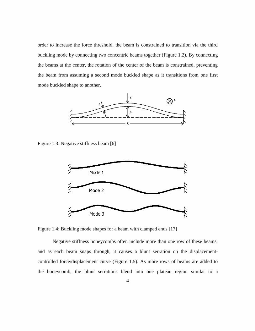
order to increase the force threshold, the beam is constrained to transition via the third
buckling mode by connecting two concentric beams together (Figure 1.2). By connecting
the beams at the center, the rotation of the center of the beam is constrained, preventing
the beam from assuming a second mode buckled shape as it transitions from one first
mode buckled shape to another.
Figure 1.3: Negative stiffness beam [6]
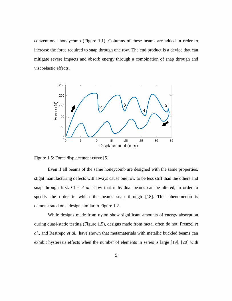
Figure 1.4: Buckling mode shapes for a beam with clamped ends [17]
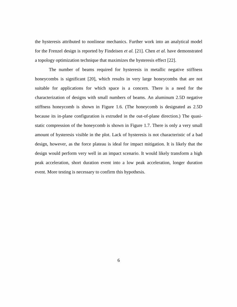
Negative stiffness honeycombs often include more than one row of these beams,
and as each beam snaps through, it causes a blunt serration on the displacement-
controlled force/displacement curve (Figure 1.5). As more rows of beams are added to
the honeycomb, the blunt serrations blend into one plateau region similar to a
5
conventional honeycomb (Figure 1.1). Columns of these beams are added in order to
increase the force required to snap through one row. The end product is a device that can
mitigate severe impacts and absorb energy through a combination of snap through and
viscoelastic effects.
Figure 1.5: Force displacement curve [5]
Even if all beams of the same honeycomb are designed with the same properties,
slight manufacturing defects will always cause one row to be less stiff than the others and
snap through first. Che et al. show that individual beams can be altered, in order to
specify the order in which the beams snap through [18]. This phenomenon is
demonstrated on a design similar to Figure 1.2.
While designs made from nylon show significant amounts of energy absorption
during quasi-static testing (Figure 1.5), designs made from metal often do not. Frenzel et
al., and Restrepo et al., have shown that metamaterials with metallic buckled beams can
exhibit hysteresis effects when the number of elements in series is large [19], [20] with
6
the hysteresis attributed to nonlinear mechanics. Further work into an analytical model
for the Frenzel design is reported by Findeisen et al. [21]. Chen et al. have demonstrated
a topology optimization technique that maximizes the hysteresis effect [22].
The number of beams required for hysteresis in metallic negative stiffness
honeycombs is significant [20], which results in very large honeycombs that are not
suitable for applications for which space is a concern. There is a need for the
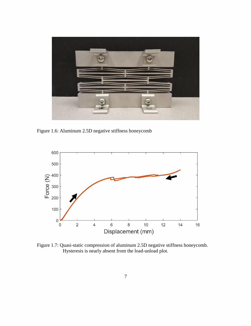
characterization of designs with small numbers of beams. An aluminum 2.5D negative
stiffness honeycomb is shown in Figure 1.6. (The honeycomb is designated as 2.5D
because its in-plane configuration is extruded in the out-of-plane direction.) The quasi-
static compression of the honeycomb is shown in Figure 1.7. There is only a very small
amount of hysteresis visible in the plot. Lack of hysteresis is not characteristic of a bad
design, however, as the force plateau is ideal for impact mitigation. It is likely that the
design would perform very well in an impact scenario. It would likely transform a high
peak acceleration, short duration event into a low peak acceleration, longer duration
event. More testing is necessary to confirm this hypothesis.
7
Figure 1.6: Aluminum 2.5D negative stiffness honeycomb
Figure 1.7: Quasi-static compression of aluminum 2.5D negative stiffness honeycomb.
Hysteresis is nearly absent from the load-unload plot.
8
The 2.5D design illustrated in Figure 1.2 has some drawbacks. On a flat surface
when subject to in-plane mechanical loading that is perfectly orthogonal to its top
surface, it mitigated impacts very well, but out-of-plane or shear loading can induce out-
of-plane bending in the honeycomb, which may cause it to fail. There is a need for a
negative stiffness design that can conform to curved surfaces and accommodate out-of-
plane mechanical loading.
Negative stiffness elements have the potential for protecting components from
severe impacts. National laboratories such as Sandia National Laboratories have
components that require protection from impacts as high as 15,000 G, at durations in the
tenths of milliseconds. Because of the potential for high temperatures, polymer closed
cell foams cannot be used. Metal foams cannot be used either, as they are not elastically
recoverable. Multiple negative stiffness elements could be used together in a cohesive
design to protect these components. There is a need to develop this multi-element
conformal assembly and to investigate its quasi-static and dynamic mechanical behavior.
These types of negative stiffness honeycombs need to be accurately and
efficiently modeled. Analytical equations, such as those developed by Qiu et al. [17],
approximate the behavior of negative stiffness elements, but they do not account for
important practical factors such as non-rigid boundary conditions and high-speed
impacts. The analytical equations also model the post buckling behavior poorly. The snap
through of the beams is often a dynamic event, with rapidly changing loads and rigid
body motion. A better approach to modeling the beams is to use finite element analysis
(FEA). With FEA, if accurate post buckling behavior is desired, an explicit solution could
be used that accounts for rigid body motion. For quasi-static analysis, the modified-Riks
9
method could be used to model the force-displacement behavior of a beam as it
transitions from one first-mode buckled shape to another. Izard et al. use a Riks algorithm
to confirm analytical models [23]. These methods provide the potential for acceptable
accuracy with minimal computational expense.
To validate the FEA models, they could be compared to physical experiments.
Specimens with a varied number of rows and columns could be fabricated and subjected
to static and dynamic mechanical experiments, and then compared to FEA results.
Repeatability could be investigated by testing an element multiple times and tracking
shifts in behavior. These tests could include quasi-static tests and dynamic drop-tests. The
drop-tests could consist of a simple plate of specified mass, falling onto the negative
stiffness element. By measuring the velocity at the moment before impact, the drop-test
could be accurately replicated in FEA using a dynamic explicit simulation.
Dynamic testing of negative stiffness elements needs to be conducted to
investigate their behavior under extreme impulses. The elements could be designed in
FEA software using a parametric model that matches the conditions found in the actual
test. The elements could then be tested using a commercial drop-test rig that is capable of
extremely high G impulses at short durations. The tests could then be compared to the
FEA using accelerometer data and high speed camera video.
AM provides an economical way of producing functional design prototypes.
Using selective laser sintering and direct metal laser sintering, material properties similar
to polymer injection molding and metal casting, respectively, can be achieved. The parts
fabricated by the AM machines are not always perfect, however, and can exhibit defects
in terms of material strength, geometric scaling, porosity, warping, etc. [24], [25], [26].
10
There is a need for a model that incorporates these sources of variability and outputs a
range of performance for a given design.
1.2: RESEARCH GOALS
The negative stiffness honeycomb design will be studied in depth, to include a
new conformal design. Quasi-static compression tests, dynamic impact tests, and
dynamic impulse tests will be conducted to evaluate the performance of the honeycombs
and to validate and refine FEA models. Material and geometry variation will be
incorporated into a model that predicts force threshold for a given design. To show the
true potential of the conformal design a multi-element test will be conducted, and
compared against an FEA model.
Goal 1: Design a conformal negative stiffness element that protects objects with
curved surfaces.
If a conventional 2.5D negative stiffness element is used on a curved surface, an
impact is likely to damage the element because the load is not in-plane and orthogonal to
the top surface of the element. A conformal negative stiffness element design will be
introduced that can conform to curved surfaces and protect against angled impacts.
Goal 2: Conduct quasi-static and dynamic FEA of the 2.5D and conformal designs
to predict quasi-static and impact performance.
It is important to be able to simulate the behavior of the negative stiffness
honeycombs prior to manufacture to reduce the need for iterative prototyping. A
parametric model will be built in FEA, to allow for quick design iterations or
optimization. Abaqus® FEA software allows for parametric models to be built using the
Python scripting language. The implementation has the full functionality of the Python
11
language, including external packages. Designs can be considered objects, with their own
variables and functions. Then, each design can be simulated with Abaqus® FEA explicit
dynamic analysis or Riks analysis for quasi-static or dynamic simulations, respectively.
Shell elements, symmetry, and other techniques can also be used to reduce the
computational expense of the analyses. This automated simulation capability allows the
designer to quickly iterate through designs and extract useful analysis data.
Goal 3: Conduct quasi-static and dynamic testing of 2.5D and conformal negative
stiffness designs to evaluate impact performance.
The 2.5D and conformal designs will be tested quasi-statically using a simple
compression testing frame. These experiments will be used to validate and refine the FEA
model. The force-displacement relationship will be recorded for repeated test cycles,
which will uncover any hysteresis between cycles. Dynamic testing will consist of
dropping a known mass onto the element from a prescribed height. The velocity prior to
impact will be recorded and used as input to the FEA simulation. The results of the
simulation and experiments will then be compared to validate the simulation models.
Goal 4: Conduct dynamic impulse testing at Sandia National Laboratories to
evaluate the performance of conformal negative stiffness honeycombs under high
acceleration impulses.
The conformal designs will be bolted to a drop-table, hoisted into the air, and
dropped at a prescribed height. Onboard accelerometers will capture the response of the
element, which will then be compared to FEA simulations. A state-of-the-art high speed
camera will be used to visualize the behavior of the elements during testing.
12
Goal 5: Model the manufacturing-induced variability in the conformal negative
stiffness honeycombs to evaluate the predictability and reliability of their impact
performance.
Additive manufacturing results in a high degree of material property variability
and can result in geometric distortions. Sources of variability from the additive process
will be quantified and incorporated into an FE model that predicts the force threshold for
a given design, resulting in a stochastic simulation of the force threshold. To evaluate the
shape and scale of the geometric distortions, a Computed Tomography (CT) study will be
conducted. The 3D image from the CT study will then be used to map imperfections onto
the FEA model.
Goal 6: Conduct multi-element testing to evaluate performance under more
realistic conditions.
A multi-element test will investigate the conformal honeycomb’s ability to
conform to a curved surface and provide multi-element impact mitigation. Testing will be
conducted quasi-statically at UT Austin, and dynamically at Sandia National
Laboratories. Results will be compared to a multi-element finite element model.
1.3: CHAPTER SUMMARY
Chapter 2: Methods of Analysis
This chapter will describe methods for analyzing the quasi-static and dynamic
mechanical behavior of the negative stiffness honeycombs. It will begin by describing
analytical and empirical relationships for evaluating the force threshold. Then, the
parametric FEA framework will be described, including how it was designed and
implemented, and how important it is for simulation and manufacture. This will lead into
13
a discussion of quasi-static FEA for generating the force-displacement profile of a
specific design followed by dynamic FEA for simulating mechanical impacts.
Chapter 3: 2.5D Negative Stiffness Honeycomb Experiments
This chapter will begin with a discussion of the fabrication of the 2.5D
honeycombs. Quasi-static experimental tests for the 2.5D design will then be presented.
The results of variable row/column testing will be presented, along with an explanation of
changes in the force threshold as the rows and columns are varied. The results of dynamic
impact testing of the 2.5D design will be presented, and all results will be compared to
FEA.
Chapter 4: Conformal Negative Stiffness Honeycomb Experiments
This chapter will be similar to the 2.5D Design chapter but focused on the
conformal negative stiffness honeycombs, instead. It will include the results of dynamic
impulse experiments, as well.
Chapter 5: Predictability and Reliability Modeling
This chapter will begin with a discussion of the challenges encountered when
manufacturing negative stiffness honeycombs using an additive process. Then, it will
describe the use of computed tomography to image imperfections of an AM part and
present a procedure for mapping the results to an FEA model. The specific sources of
variability in additively manufactured specimens will be discussed, including material
properties, beam thickness, beam height and shape imperfection. Uncertainty analysis
with respect to the predicted force threshold will be conducted using latin hypercube
14
sampling and the parametric FEA code. Finally, the results of quasi-static testing will be
compared to the model for validation.
Chapter 6: Multi-Element Assembly
This chapter will begin with a discussion of how the elements are assembled to
operate as a cohesive unit. Quasi-static experiment results will be described and the
results compared with FEA predictions to demonstrate the effectiveness of the multi-
element assembly and associated FEA framework. The challenges associated with
simulating multiple elements simultaneously will be discussed. A multi-element
assembly impulse testing fixture will be discussed including how it was designed and
built. Results of dynamic impulse testing of the assembly will be described and compared
with FEA predictions.
Chapter 7: Conclusion
This chapter will summarize this dissertation. In the future work section, potential
follow-on projects such as a helmet design, fatigue testing, negative stiffness designs
incorporating dampers, and vibration dampening layers will be presented. The final
section will succinctly conclude the dissertation.
15
Analysis of Quasi-static and Dynamic Behavior of Negative
Stiffness Honeycombs
This chapter includes an overview of the analytical and finite element analysis
(FEA) methods used to characterize the quasi-static and dynamic behavior of negative
stiffness honeycombs.
2.1: NEGATIVE STIFFNESS HONEYCOMB DESIGNS
2.5D Negative Stiffness Honeycomb
The 2.5D negative stiffness honeycomb is a two dimensional design that
incorporates curved beams that buckle elastically (Figure 2.1). The 2.5D designation
describes the two-dimensional cross-section of the design which is extruded to a specified
depth. Increasing the depth results in a higher force threshold. The design is scalable by
adding more rows or columns. Curved beams are supported by adjacent beams, a straight
center beam, and a side block called a bumper. Since these supports are made of the same
material as the beam, they deform elastically, which affects the boundary conditions of
the beams and limits their force threshold.
16
Figure 2.1: 2.5D negative stiffness honeycomb
The 2.5D honeycomb is designed primarily for vertical loading that is in the plane
of the cross-section and orthogonal to the top base plate since the honeycomb must
collapse vertically to mitigate impacts. Angled impacts introduce shear loads and cause
the honeycomb to deform in a direction that does not mitigate impacts. The 2.5D
honeycomb does not conform to curved surfaces well, either, because its base needs to
rest on a flat surface.
Conformal Negative Stiffness Honeycomb
The conformal negative stiffness honeycomb is intended to solve the problem of
conforming to curved surfaces. A 1 column, 2 row assembly of curved beams is revolved
360 degrees about its central axis to produce a 3D design. Four corners are then cut out of
the element to allow the design to be tiled together (Figure 2.2).
17
Figure 2.2: Conformal negative stiffness element
The advantages of this design are significant. Each beam is converted from a
snap-through beam to a snap-through surface, which increases its force threshold relative
to two beam-based designs occupying the same footprint because it uses the center of the
element more efficiently. Multiple elements can be assembled in a tiled pattern (Figure
2.3). This pattern can then be placed on a curved surface, to allow for impact mitigation
and energy absorption from off-axis loads.
Figure 2.3: Tiling of conformal negative stiffness elements
18
Because of the geometric complexity of the design, it is advantageous to
manufacture it using additive methods. A conventional manufacturing method would
require a multi-part assembly, which would make the part more complex and add modes
of failure. For low impact applications, the design can be fabricated in Nylon 11 using
SLS. When a design is required to have a high force threshold or withstand high
temperatures, the design can be fabricated with high yield strain metals such as 17-4
stainless steel using Direct Metal Laser Sintering (DMLS). The open nature of the design
allows for powder to escape after fabrication.
2.2: ANALYTICAL METHOD
An analytical method for determining the force threshold of a negative stiffness
beam has been developed by Qiu et al. [17]. The method assumes rigid boundary
conditions and depends on the beam thickness (t), length (L), and height (h). These
critical dimensions are shown in Figure 2.4 and Figure 2.5.
Figure 2.4: Diagram showing the critical beam dimensions and direction of force
x
y(x)
19
Figure 2.5: Section view of a conformal negative stiffness honeycomb with critical
dimensions
The conformal design shares the same beam shape as the 2.5D design (Equation
2.1),
𝑦(𝑥) =ℎ
2[1 − cos (2𝜋
𝑥
𝐿) (2.1)
with y representing the height of the beam and x the horizontal distance from the
endpoint of the beam, as illustrated in Figure 2.4. The force threshold is a function of
normalized force (𝑓) and displacement (∆), as shown in Equation 2.2. The direction of
force (F) is shown in Figure 2.4. 𝑄 is the ratio between beam height (ℎ) and beam
thickness (𝑡). Force is normalized using the Young’s modulus of the material (𝐸), the
area moment of inertia (𝐼), and the beam length and height (Equation 2.4). Displacement
is normalized using the transverse displacement and beam height (Equation 2.5).
20
𝑓 =3𝜋4𝑄2
2∆ (∆ −
3
2+ √
1
4−
4
3𝑄2) (∆ −
3
2− √
1
4−
4
3𝑄2) (2.2)
𝑄 =ℎ
𝑡 (2.3)
𝐹 =𝑓𝑙3
𝐸𝐼ℎ (2.4)
∆ = 𝑑
ℎ (2.5)
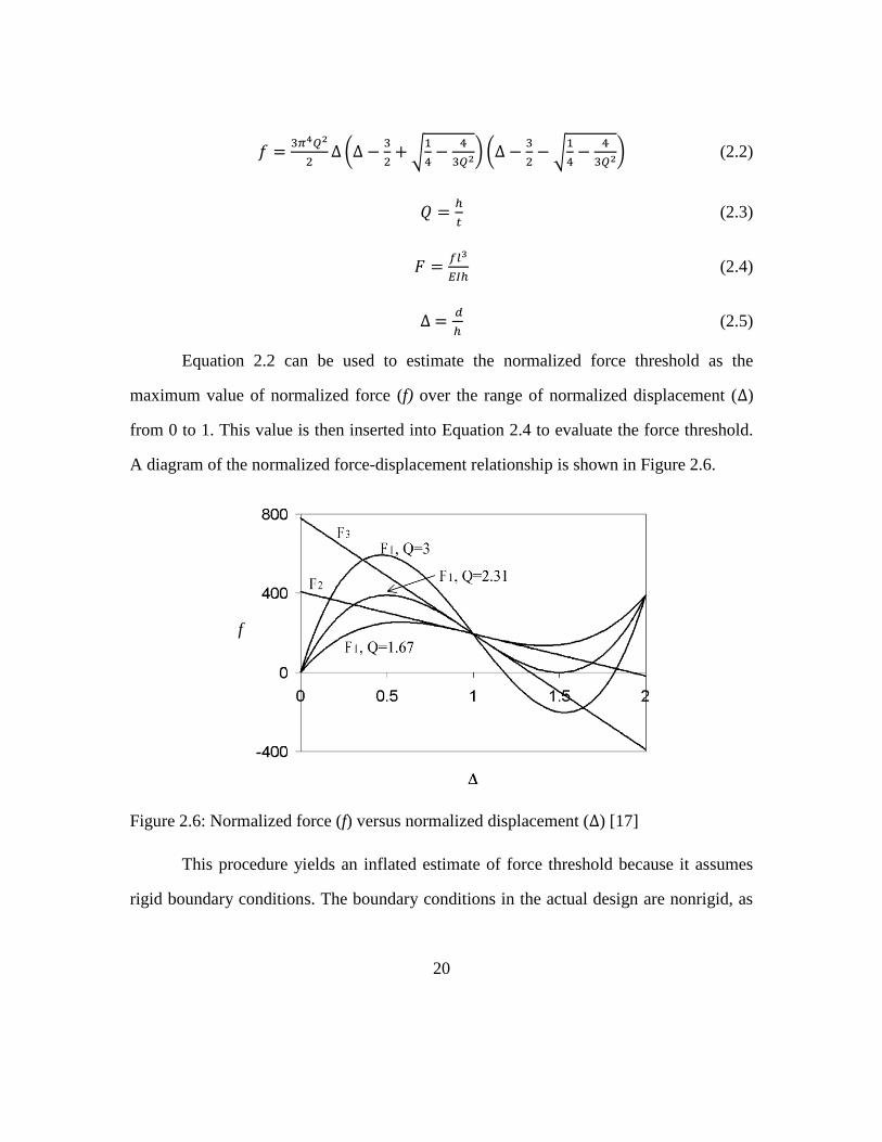
Equation 2.2 can be used to estimate the normalized force threshold as the
maximum value of normalized force (f) over the range of normalized displacement (∆)
from 0 to 1. This value is then inserted into Equation 2.4 to evaluate the force threshold.
A diagram of the normalized force-displacement relationship is shown in Figure 2.6.
Figure 2.6: Normalized force (f) versus normalized displacement (∆) [17]
This procedure yields an inflated estimate of force threshold because it assumes
rigid boundary conditions. The boundary conditions in the actual design are nonrigid, as
f
21
shown in Figure 2.1. As the beam snaps through it pushes outward on its supports,
causing them to deform.
It is also important to estimate the maximum strain in the beam during the snap
through event (Equation 2.6) [17]. This quantity can be compared with the yield strain of
the beam material to ensure that the beam does not plastically deform during the snap
through event.
𝜀𝑚𝑎𝑥 ≈ 2𝜋2 𝑡ℎ
𝐿2 + 4𝜋2 𝑡2
3𝐿2 (2.6)
Equation 2.3 has added importance as it determines whether the design will be
bistable or monostable. Theoretically, bistability (𝑄) values above 2.31 indicate
bistability [17], which means that the design will require an external force in the opposite
direction of the transverse force, F, to return to its original state following an impact or
applied transverse force. A monostable design returns to its original state on its own. It is
important for a design to be monostable if protection from multiple impacts is desired. If
a bistable design were used in such a situation, the design would offer limited mitigation
on the second impact. Since the analytical equations assume rigid boundary conditions
the bistability parameter can be increased beyond 2.31 for realistic designs, but care must
be taken to avoid bistability. The bistability parameter is usually maximized for most
designs to increase the force threshold, but it should not be set too high to avoid
bistability.
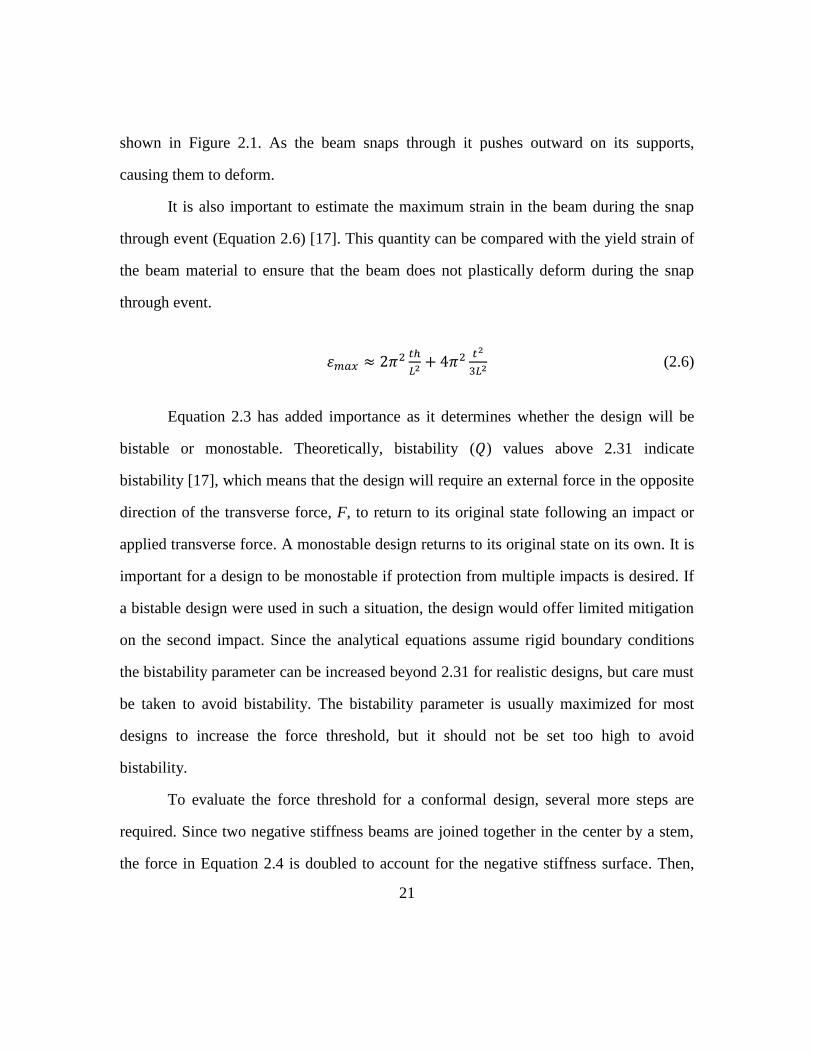
To evaluate the force threshold for a conformal design, several more steps are
required. Since two negative stiffness beams are joined together in the center by a stem,
the force in Equation 2.4 is doubled to account for the negative stiffness surface. Then,
22
the force estimated by Equation 2.4 is doubled again to account for the second concentric
beam/surface, for a total of four multipliers (Equation 2.4). The width of the beam (b) is
adjusted so that it is 2/3 the beam length (Figure 2.7). This procedure provides a rough
estimate of force threshold for the conformal design.
Figure 2.7: Top view of conformal negative stiffness design that shows how the design
can be approximated by two 2.5D designs
2.3: PARAMETRIC FEA MODEL
FEA models of the conformal negative stiffness designs are needed to predict the
quasi-static and dynamic behavior of the manufactured designs. This section focuses on
modeling the conformal honeycomb because it is more complex than the 2.5D
honeycomb. The analytical equations presented in Section 2.2 assume fixed displacement
boundaries for the negative stiffness elements, which results in higher calculated force
thresholds than those observed in fabricated specimens. Also, the equations do not take
b
23
into account the rest of the honeycomb structure, which surrounds and supports the
negative stiffness elements; nor do they accurately model the pre- and post-buckling
behavior of the honeycomb assembly. These limitations preclude them from being used
to model the entire quasi-static or dynamic loading cycle.
A fully parametric simulation has been developed using the Python scripting
language in Abaqus® to enable quick design iteration. As the designer works in
Abaqus®, all commands are recorded in Python in a journal file. This file allows the
designer to quickly learn new commands and use them in a script. Almost all
functionality in Abaqus® can be achieved using Python commands. The Abaqus®
Python modules are organized using objects and dictionaries, which allow the designer to
easily adopt standard Python programming practices when programming for Abaqus®.
The parametric simulation developed for this dissertation allows the designer to
adjust the negative stiffness honeycomb using a configuration file. The configuration file
contains all of the parameters needed to drive the simulation, including beam thickness,
beam height, and simulation type. The code builds the complete simulation, including
building part geometry, meshing the part, assigning boundary conditions, and
establishing contact interactions. Each simulation is treated as its own object in the code
which allows for quick post-processing analysis. Results from analyses are saved to an
industry standard JSON file, which allows variables to be quickly loaded into
MATLAB® or Python without the need for parsing text files. Git version control is used
to maintain simulation data integrity. Each simulation project is separated into its own
branch, in order to maintain a bug-free master repository. This allows for multiple
experimental simulation projects to be developed at the same time without harming the
24
production master code. The code is routinely synced with an industry standard GitHub
repository to allow other students to use the code in their projects.
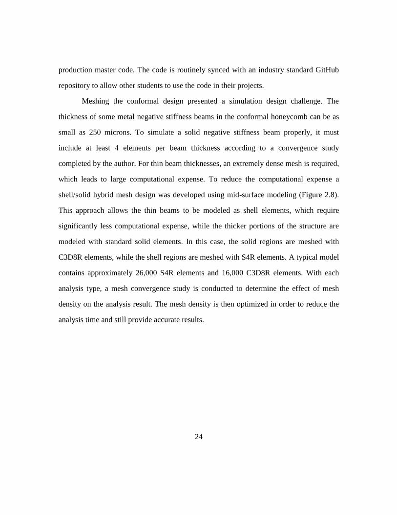
Meshing the conformal design presented a simulation design challenge. The
thickness of some metal negative stiffness beams in the conformal honeycomb can be as
small as 250 microns. To simulate a solid negative stiffness beam properly, it must
include at least 4 elements per beam thickness according to a convergence study
completed by the author. For thin beam thicknesses, an extremely dense mesh is required,
which leads to large computational expense. To reduce the computational expense a
shell/solid hybrid mesh design was developed using mid-surface modeling (Figure 2.8).
This approach allows the thin beams to be modeled as shell elements, which require
significantly less computational expense, while the thicker portions of the structure are
modeled with standard solid elements. In this case, the solid regions are meshed with
C3D8R elements, while the shell regions are meshed with S4R elements. A typical model
contains approximately 26,000 S4R elements and 16,000 C3D8R elements. With each
analysis type, a mesh convergence study is conducted to determine the effect of mesh
density on the analysis result. The mesh density is then optimized in order to reduce the
analysis time and still provide accurate results.
25
Figure 2.8: Shell/Solid hybrid model of conformal design
2.4: QUASI-STATIC FEA
The parametric simulation enables quasi-static analysis using the modified-Riks
method [27]. This method solves for the force displacement curve in increments of arc
length, generating force-displacement curves that match the shape of the actual test data.
The modified-Riks method is necessary due to the presence of model instability when the
beams snap from one curved shape to another. If a standard FEA were applied, the load
and displacement would increase together until the force plateaued near the snap-through
region. Then, the load would drop significantly, which would cause the simulation to
crash. The modified-Riks method can account for this instability by using a variable load.
The designer sets up the simulation as they would for a standard simulation, but instead
of applying a displacement boundary condition, the designer applies a load to the top of
the element. The load is typically set to a value larger than the maximum load required
for snap through. The load is multiplied by a scalar, called the Load Proportionality
26
Factor (LPF) to calculate the actual applied load for each step of the simulation. This
scalar is varied by the modified-Riks method to evaluate equilibrium displacement as the
load is increased. When the simulation starts, the LPF is set to an initial value, which
causes the element to displace a certain amount. The simulation progresses in increments
of arc length, solving for the LPF and displacement as it goes.
Care must be taken when setting the maximum arc length increment, as with
complex problems such as negative stiffness elements, the load-displacement curve can
take multiple paths. If the increment is too large, the element may take a simplified
loading path. If the snap through is too violent, the modified-Riks method finds a path
that is smoother than the actual result.
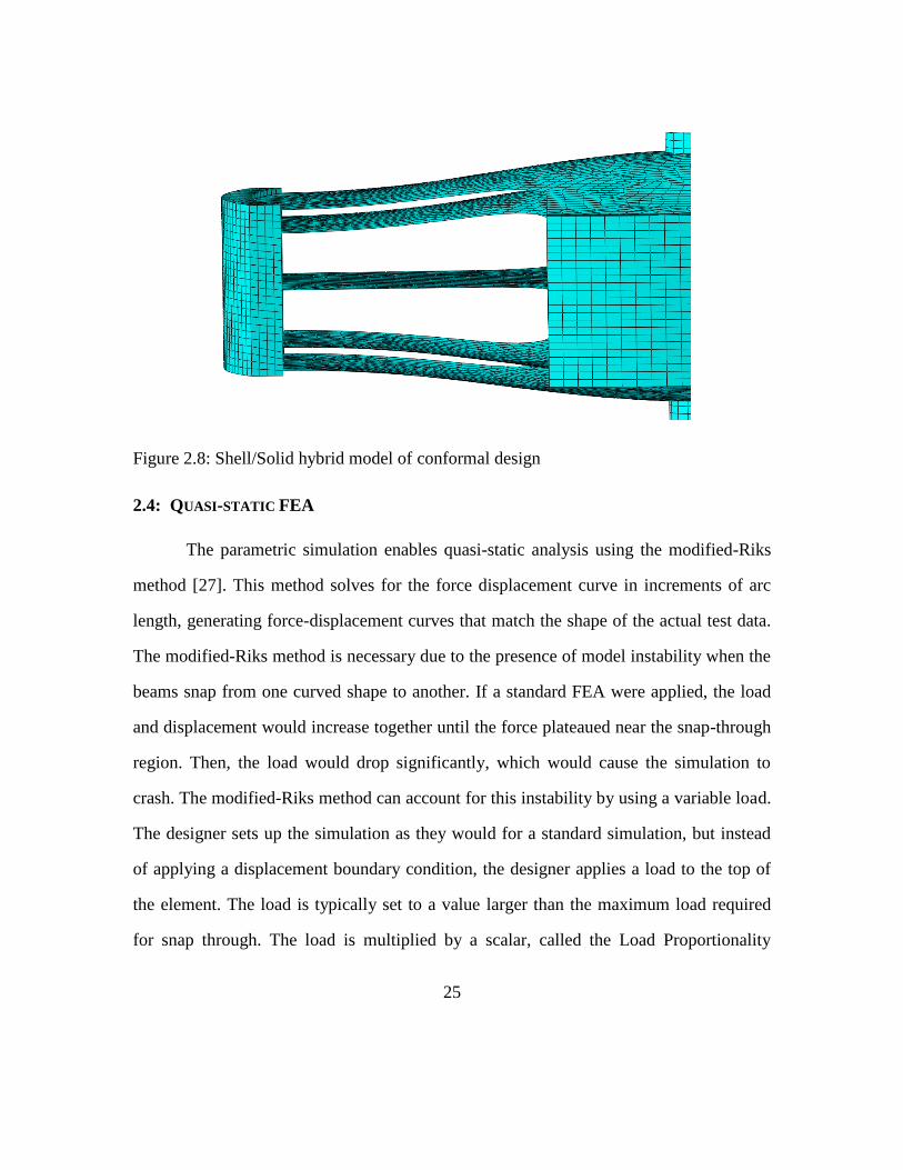
Figure 2.9 illustrates the boundary conditions for the conformal design. Vertical
displacement is fixed along the bottom surface, but in-plane displacements are permitted.
Several nodes are fixed on the bottom surface in order to prevent rigid body translation.
These conditions minimally constrain the model and prevent unrealistic concentrations of
stress. A pressure load is applied to the top surface of the model, including both solid and
shell surfaces.
27
Figure 2.9: Boundary conditions for FEA of conformal design
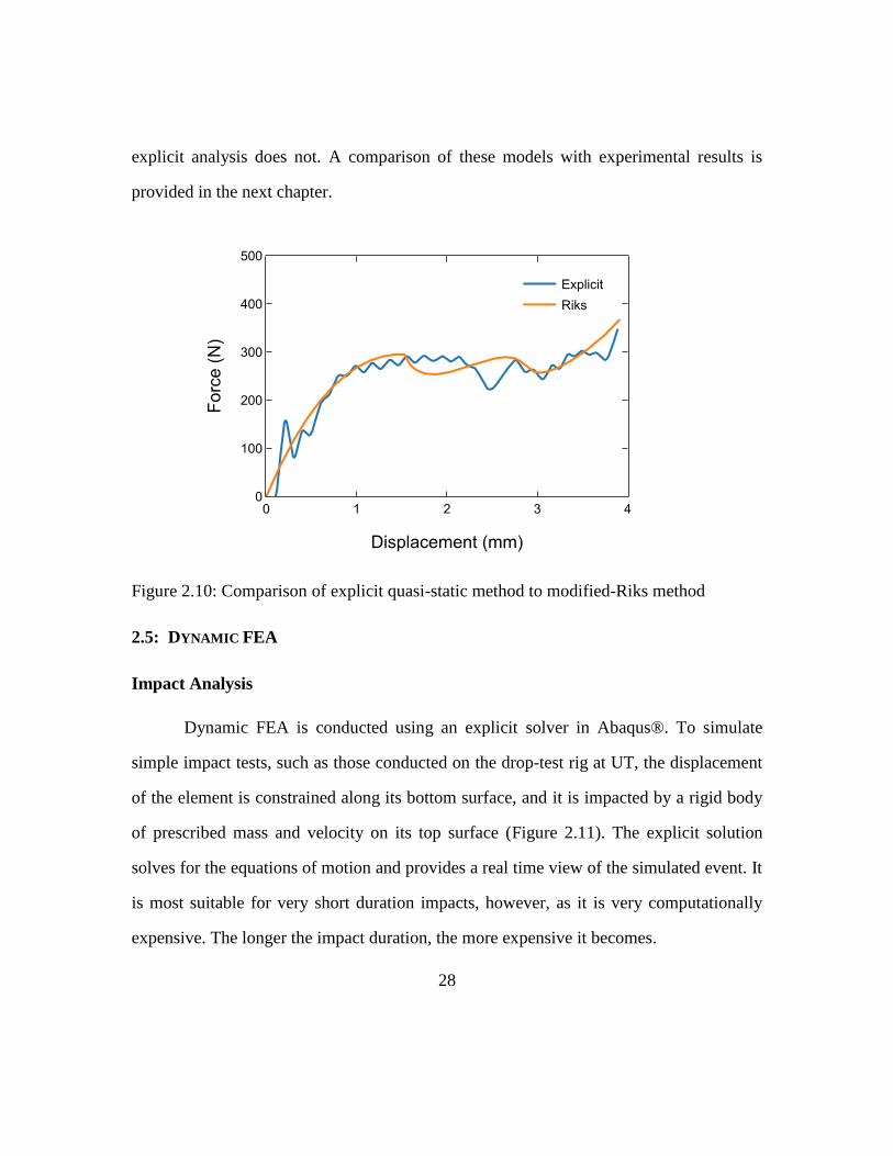
The modified-Riks method performs quite well when compared to an explicit
quasi-static analysis (Figure 2.10) for a conformal negative stiffness honeycomb with a
beam thickness, height, and length of 0.40, 1.02, and 37.50 mm, respectively. The
explicit analysis required 17 hours and 56 minutes of computational time on a 16 core
server while the Riks analysis took only 1 hour and 46 minutes. The explicit analysis also
required a 4th order, 5 kHz cut off frequency, forward and backward Butterworth filter, to
remove significant noise, indicating that the explicit analysis could have benefitted from
a reduction in the time step, which would add even more computational expense. The
Riks analysis requires no filtering and yields a very smooth force-displacement curve.
The Riks analysis also shows the two characteristic negative stiffness serrations while the
Bottom Surface fixed in Z / several nodes at center fixed in XYZ
+Z
Pressure Load
+X
+Y
28
explicit analysis does not. A comparison of these models with experimental results is
provided in the next chapter.
Figure 2.10: Comparison of explicit quasi-static method to modified-Riks method
2.5: DYNAMIC FEA
Impact Analysis
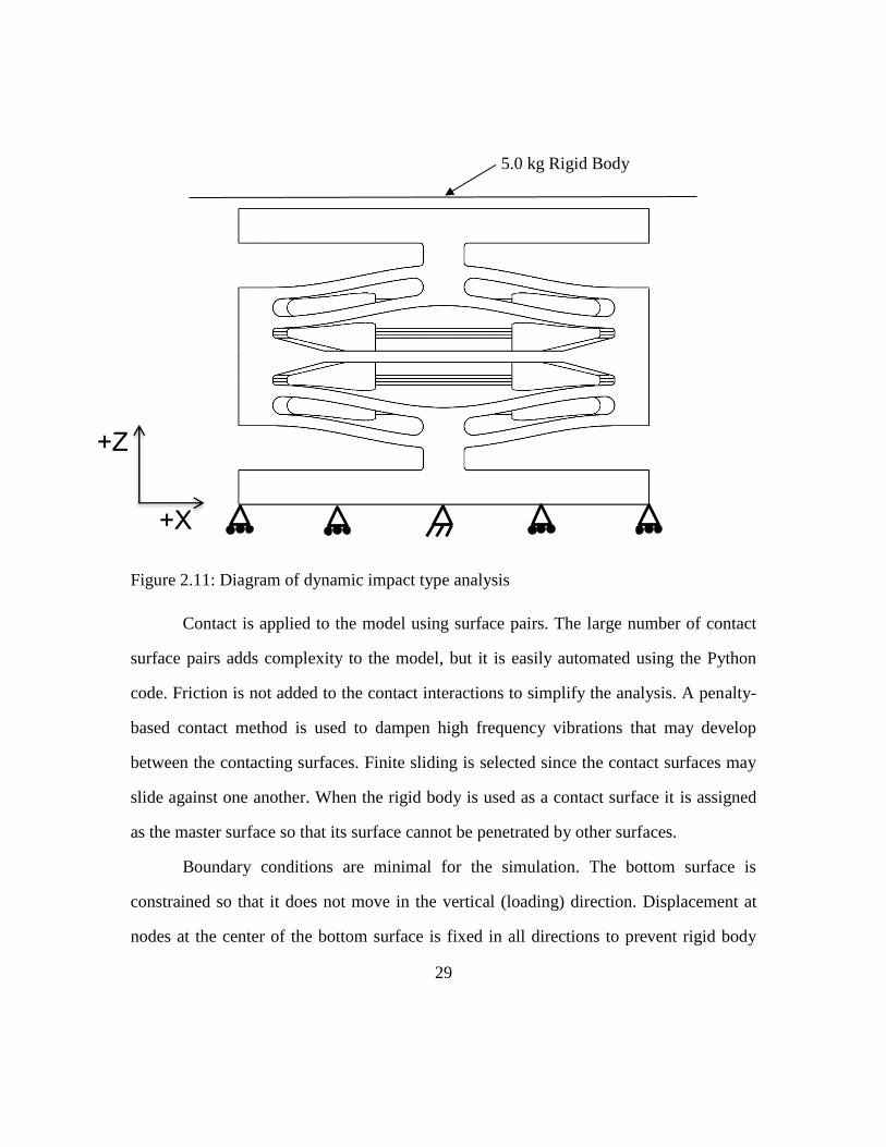
Dynamic FEA is conducted using an explicit solver in Abaqus®. To simulate
simple impact tests, such as those conducted on the drop-test rig at UT, the displacement
of the element is constrained along its bottom surface, and it is impacted by a rigid body
of prescribed mass and velocity on its top surface (Figure 2.11). The explicit solution
solves for the equations of motion and provides a real time view of the simulated event. It
is most suitable for very short duration impacts, however, as it is very computationally
expensive. The longer the impact duration, the more expensive it becomes.
29
Figure 2.11: Diagram of dynamic impact type analysis
Contact is applied to the model using surface pairs. The large number of contact
surface pairs adds complexity to the model, but it is easily automated using the Python
code. Friction is not added to the contact interactions to simplify the analysis. A penalty-
based contact method is used to dampen high frequency vibrations that may develop
between the contacting surfaces. Finite sliding is selected since the contact surfaces may
slide against one another. When the rigid body is used as a contact surface it is assigned
as the master surface so that its surface cannot be penetrated by other surfaces.
Boundary conditions are minimal for the simulation. The bottom surface is
constrained so that it does not move in the vertical (loading) direction. Displacement at
nodes at the center of the bottom surface is fixed in all directions to prevent rigid body
5.0 kg Rigid Body
+Z
+X
30
motion, but the rest of the nodes are allowed to expand in the plane parallel to the
surface. The rigid body impacting the honeycomb is allowed to move only in the loading
direction orthogonal to the top surface of the honeycomb, and it is assigned a prescribed
velocity. At the beginning of the simulation, it is placed 0.01 mm from the top surface of
the negative stiffness element to minimize the amount of free fall time and reduce the
computational resources required for the simulation. Gravity loads are applied to the rigid
body, but they do not affect the results significantly because of the large velocity of the
impact.
The analysis time of the simulation is adjusted to capture the entire impact event.
If the prescribed velocity of the rigid body is small, then the simulation takes longer to
complete.
The displacement, velocity and acceleration of the rigid body are recorded for the
duration of the simulation. These variables can be filtered later and compared to
experimental results.
Impulse Analysis
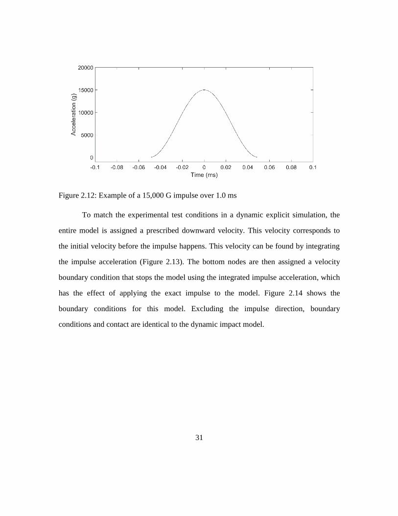
The dynamic explicit solver is also used for simulating impulse tests. In an
experimental impulse test, an impulse is applied to the specimen using a special drop rig.
The specimen is typically mounted to the top of a large aluminum carriage which rides on
rails. The carriage is lifted into the air and dropped onto a reaction mass. The impulse that
results from this impact is transferred to the specimen. The details of the experiment are
described in Chapter 4, but an example impulse is shown in Figure 2.12.
31
Figure 2.12: Example of a 15,000 G impulse over 1.0 ms
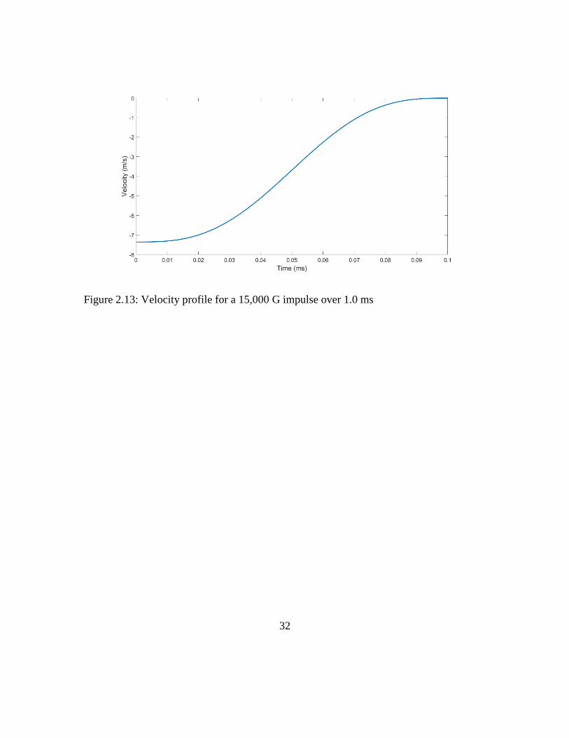
To match the experimental test conditions in a dynamic explicit simulation, the
entire model is assigned a prescribed downward velocity. This velocity corresponds to
the initial velocity before the impulse happens. This velocity can be found by integrating
the impulse acceleration (Figure 2.13). The bottom nodes are then assigned a velocity
boundary condition that stops the model using the integrated impulse acceleration, which
has the effect of applying the exact impulse to the model. Figure 2.14 shows the
boundary conditions for this model. Excluding the impulse direction, boundary
conditions and contact are identical to the dynamic impact model.
32
Figure 2.13: Velocity profile for a 15,000 G impulse over 1.0 ms
33
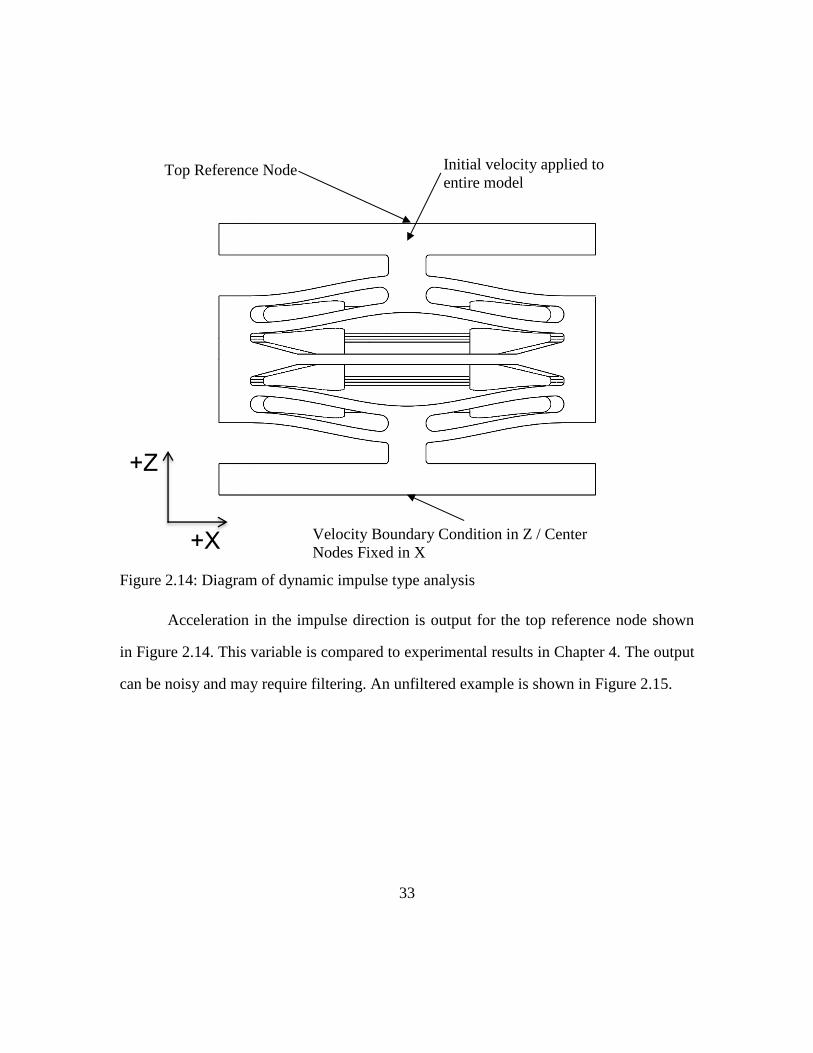
Figure 2.14: Diagram of dynamic impulse type analysis
Acceleration in the impulse direction is output for the top reference node shown
in Figure 2.14. This variable is compared to experimental results in Chapter 4. The output
can be noisy and may require filtering. An unfiltered example is shown in Figure 2.15.
Top Reference Node
Velocity Boundary Condition in Z / Center
Nodes Fixed in X
Initial velocity applied to
entire model
+Z
+X
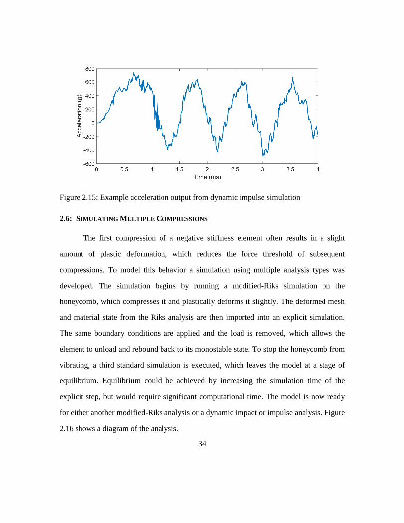
34
Figure 2.15: Example acceleration output from dynamic impulse simulation
2.6: SIMULATING MULTIPLE COMPRESSIONS
The first compression of a negative stiffness element often results in a slight
amount of plastic deformation, which reduces the force threshold of subsequent
compressions. To model this behavior a simulation using multiple analysis types was
developed. The simulation begins by running a modified-Riks simulation on the
honeycomb, which compresses it and plastically deforms it slightly. The deformed mesh
and material state from the Riks analysis are then imported into an explicit simulation.
The same boundary conditions are applied and the load is removed, which allows the
element to unload and rebound back to its monostable state. To stop the honeycomb from
vibrating, a third standard simulation is executed, which leaves the model at a stage of
equilibrium. Equilibrium could be achieved by increasing the simulation time of the
explicit step, but would require significant computational time. The model is now ready
for either another modified-Riks analysis or a dynamic impact or impulse analysis. Figure
2.16 shows a diagram of the analysis.
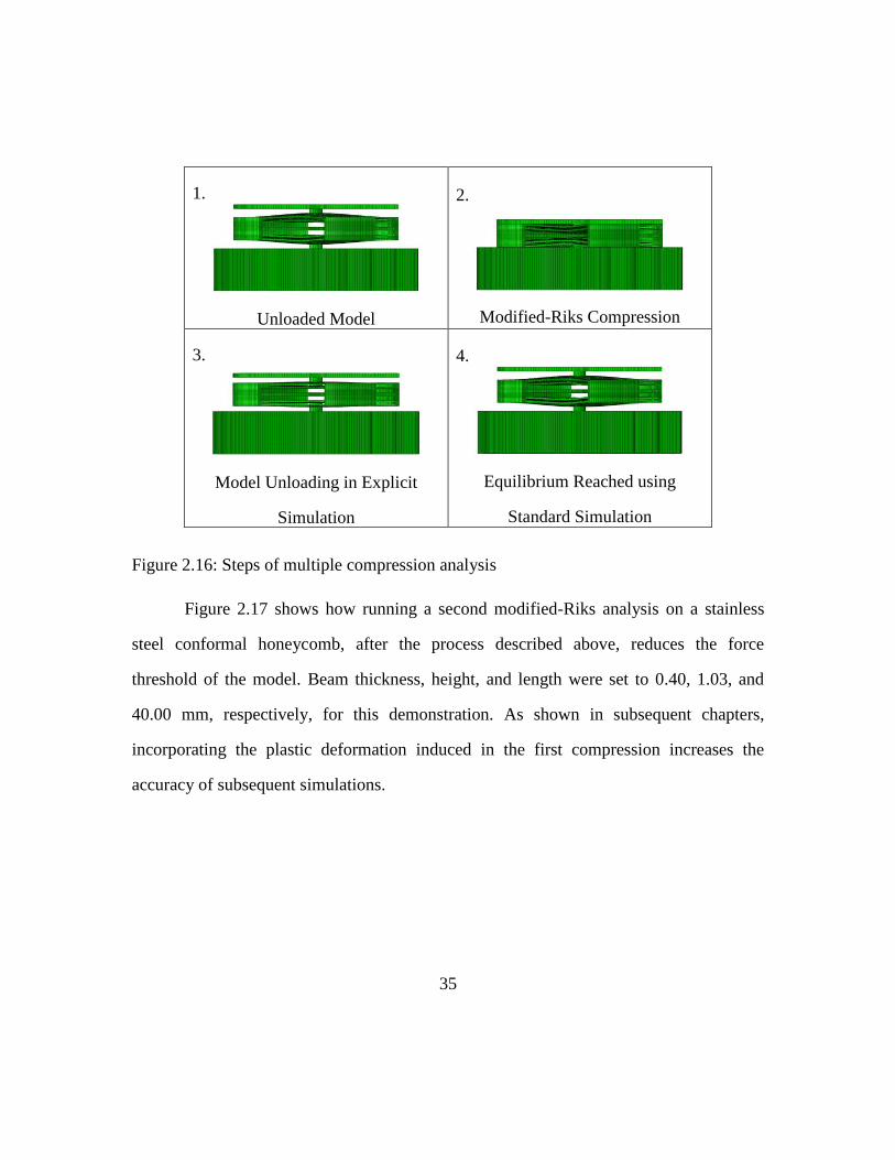
35
1.
Unloaded Model
2.
Modified-Riks Compression
3.
Model Unloading in Explicit
Simulation
4.
Equilibrium Reached using
Standard Simulation
Figure 2.16: Steps of multiple compression analysis
Figure 2.17 shows how running a second modified-Riks analysis on a stainless
steel conformal honeycomb, after the process described above, reduces the force
threshold of the model. Beam thickness, height, and length were set to 0.40, 1.03, and
40.00 mm, respectively, for this demonstration. As shown in subsequent chapters,
incorporating the plastic deformation induced in the first compression increases the
accuracy of subsequent simulations.
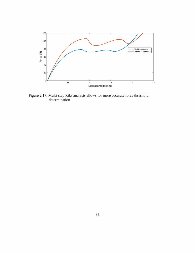
36
Figure 2.17: Multi-step Riks analysis allows for more accurate force threshold
determination

37
2.5D Negative Stiffness Honeycomb Experiments
The 2.5D negative stiffness honeycomb is characterized by an arrangement of
curved beams in rows and columns in a two-dimensional cross section, which is extruded
out of the plane to a specified depth. Depth is designated by (b) in Figure 3.1. Increasing
the depth has the effect of increasing the force threshold, or the force required to snap
through the beam from one first-mode buckled shape to another. Figure 3.2 shows the
quasi-static compression of a 4 row, 2 column 2.5D design. The beams are designed
using the parametric FEA code explained in the previous chapter and manufactured using
conventional and additive methods.
Figure 3.1: Depth of 2.5D design is designated by (b)
Figure 3.2: Negative Stiffness Honeycomb under Compression [5]
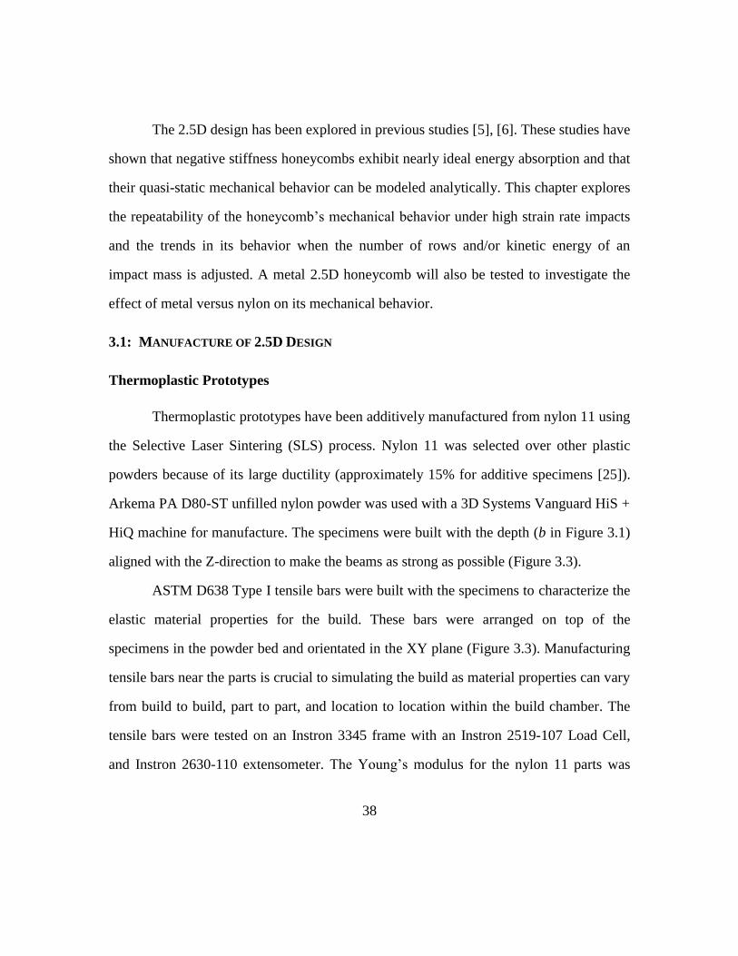
38
The 2.5D design has been explored in previous studies [5], [6]. These studies have
shown that negative stiffness honeycombs exhibit nearly ideal energy absorption and that
their quasi-static mechanical behavior can be modeled analytically. This chapter explores
the repeatability of the honeycomb’s mechanical behavior under high strain rate impacts
and the trends in its behavior when the number of rows and/or kinetic energy of an
impact mass is adjusted. A metal 2.5D honeycomb will also be tested to investigate the
effect of metal versus nylon on its mechanical behavior.
3.1: MANUFACTURE OF 2.5D DESIGN
Thermoplastic Prototypes
Thermoplastic prototypes have been additively manufactured from nylon 11 using
the Selective Laser Sintering (SLS) process. Nylon 11 was selected over other plastic
powders because of its large ductility (approximately 15% for additive specimens [25]).
Arkema PA D80-ST unfilled nylon powder was used with a 3D Systems Vanguard HiS +
HiQ machine for manufacture. The specimens were built with the depth (b in Figure 3.1)
aligned with the Z-direction to make the beams as strong as possible (Figure 3.3).
ASTM D638 Type I tensile bars were built with the specimens to characterize the
elastic material properties for the build. These bars were arranged on top of the
specimens in the powder bed and orientated in the XY plane (Figure 3.3). Manufacturing
tensile bars near the parts is crucial to simulating the build as material properties can vary
from build to build, part to part, and location to location within the build chamber. The
tensile bars were tested on an Instron 3345 frame with an Instron 2519-107 Load Cell,
and Instron 2630-110 extensometer. The Young’s modulus for the nylon 11 parts was
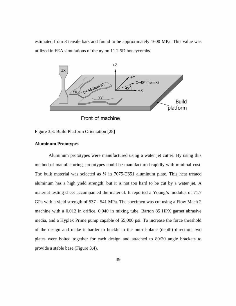
39
estimated from 8 tensile bars and found to be approximately 1600 MPa. This value was
utilized in FEA simulations of the nylon 11 2.5D honeycombs.
Figure 3.3: Build Platform Orientation [28]
Aluminum Prototypes
Aluminum prototypes were manufactured using a water jet cutter. By using this
method of manufacturing, prototypes could be manufactured rapidly with minimal cost.
The bulk material was selected as ¼ in 7075-T651 aluminum plate. This heat treated
aluminum has a high yield strength, but it is not too hard to be cut by a water jet. A
material testing sheet accompanied the material. It reported a Young’s modulus of 71.7
GPa with a yield strength of 537 - 541 MPa. The specimen was cut using a Flow Mach 2
machine with a 0.012 in orifice, 0.040 in mixing tube, Barton 85 HPX garnet abrasive
media, and a Hyplex Prime pump capable of 55,000 psi. To increase the force threshold
of the design and make it harder to buckle in the out-of-plane (depth) direction, two
plates were bolted together for each design and attached to 80/20 angle brackets to
provide a stable base (Figure 3.4).
40
Figure 3.4: Aluminum 2.5D honeycomb showing the 80/20 angle brackets used to
support the design
3.2: DESIGN CONSIDERATIONS
The as-built properties of the aluminum and nylon designs are shown in Table
3.1. The properties are the average of several caliper measurements with a precision of
+/- 0.01 mm. However, it is important to note that the surface roughness of the nylon
specimens can increase the measurement by as much as 0.07 mm relative to the
dimension of the underlying bulk part [29]. Due to the accuracy of the additive and water
jet processes, the as-designed properties differ from the as-built properties. Care must be
taken during fabrication to ensure that the as-built properties do not result in a beam with
significant plastic deformation or bistability.
For the aluminum specimens a beam thickness of 1.00 mm was chosen because it
is the smallest thickness the water jet machine could cut reliably. The minimum thickness
for metal designs is chosen because it decreases the maximum elastic strain in the beams
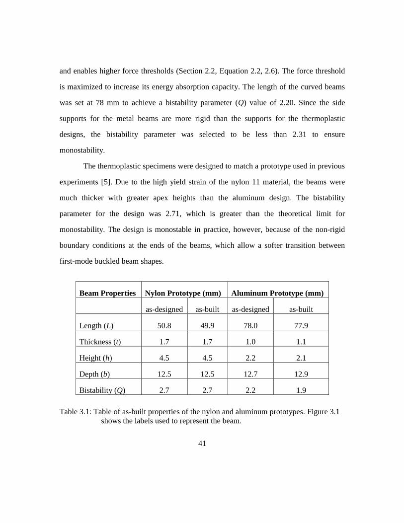
41
and enables higher force thresholds (Section 2.2, Equation 2.2, 2.6). The force threshold
is maximized to increase its energy absorption capacity. The length of the curved beams
was set at 78 mm to achieve a bistability parameter (Q) value of 2.20. Since the side
supports for the metal beams are more rigid than the supports for the thermoplastic
designs, the bistability parameter was selected to be less than 2.31 to ensure
monostability.
The thermoplastic specimens were designed to match a prototype used in previous
experiments [5]. Due to the high yield strain of the nylon 11 material, the beams were
much thicker with greater apex heights than the aluminum design. The bistability
parameter for the design was 2.71, which is greater than the theoretical limit for
monostability. The design is monostable in practice, however, because of the non-rigid
boundary conditions at the ends of the beams, which allow a softer transition between
first-mode buckled beam shapes.
Beam Properties Nylon Prototype (mm) Aluminum Prototype (mm)
as-designed as-built as-designed as-built
Length (L) 50.8 49.9 78.0 77.9
Thickness (t) 1.7 1.7 1.0 1.1
Height (h) 4.5 4.5 2.2 2.1
Depth (b) 12.5 12.5 12.7 12.9
Bistability (Q) 2.7 2.7 2.2 1.9
Table 3.1: Table of as-built properties of the nylon and aluminum prototypes. Figure 3.1
shows the labels used to represent the beam.
42
3.3: QUASI-STATIC COMPRESSION TESTING OF 2.5D HONEYCOMBS
Quasi-static compression testing was conducted on the 2.5D prototypes to
determine their force-displacement behavior and force thresholds. The testing was
conducted using an MTS Sintech 2G, 100 kN load frame, with a 100 kN Sintech 3187-
104 load cell, at room temperature. A datasheet for the load cell was unavailable, but load
cells of the same type have a repeatability of 0.02% times the full scale load [30], which
results in a precision of +/- 20 N. The prototypes were aligned with the crosshead of the
machine and compressed with a solid platen. The test progressed at a fixed speed of 2
mm/min to a specified displacement. The displacement was selected so that the machine
would reverse direction immediately after the last row of beams snapped through to its
alternative first-mode-buckled shape. The displacement limit and the slow speed of the
test were selected in order to minimize the likelihood of a load spike that could damage
the machine and load cell. Force, displacement and elapsed time were measured by the
machine and recorded for each test. Due to the rigidity of the load frame, displacement
was measured using the cross-head displacement.
Metal Prototype
Figure 3.5 shows the quasi-static force-displacement behavior for the aluminum
prototype. The plot shows a significant plateau stress, but no negative stiffness. The lack
of negative stiffness can be attributed to the low bistability parameter of 2.20. Designs
with a higher bistability parameter would demonstrate negative stiffness, but may also be
bistable. The presence of a plateau stress is nearly idea for impact mitigation, however
[1], because it indicates that the mechanical energy is absorbed at a nearly-constant force
or acceleration level.
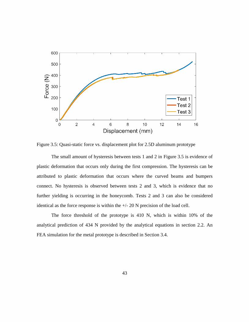
43
Figure 3.5: Quasi-static force vs. displacement plot for 2.5D aluminum prototype
The small amount of hysteresis between tests 1 and 2 in Figure 3.5 is evidence of
plastic deformation that occurs only during the first compression. The hysteresis can be
attributed to plastic deformation that occurs where the curved beams and bumpers
connect. No hysteresis is observed between tests 2 and 3, which is evidence that no
further yielding is occurring in the honeycomb. Tests 2 and 3 can also be considered
identical as the force response is within the +/- 20 N precision of the load cell.
The force threshold of the prototype is 410 N, which is within 10% of the
analytical prediction of 434 N provided by the analytical equations in section 2.2. An
FEA simulation for the metal prototype is described in Section 3.4.
44
Thermoplastic Prototype
Figure 3.6 illustrates the quasi-static force-displacement behavior of the
thermoplastic prototype. The prototype shows a blunt serration for every beam snap-
through event. The significant negative stiffness is due to the high bistability parameter
(Q) of the design (2.71). As with the aluminum design, there is some loss of force
threshold between the first and second compression that may be the result of plastic
deformation in the corners between the beams and supports.
The analytical equations predict a force threshold of 208 N which is within 2% of
the experimental force threshold of 210 N for the first compression. A modified-Riks
simulation shows blunt serrations similar to those found in the experimental test. The
experimental force threshold is slightly higher than the simulated force threshold of 175
N, however. This discrepancy is likely due to variation in the manufacturing process.
With SLS, geometric and material properties are known to vary from location to location,
build to build, and part to part [25]. An uncertainty analysis is presented in Chapter 5
that takes into account several sources of variability and predicts the force threshold for a
given design.

45
Figure 3.6: Quasi-static force vs. displacement plot for 2.5D nylon prototype
3.4: DYNAMIC IMPACT TESTING OF 2.5D HONEYCOMBS
Dynamic impact testing was conducted at UT using a customized drop rig (Figure
3.7). This rig enables testing at strain rates in the 101 to 102 s-1 range. The drop rig utilizes
an 80/20 frame member as a vertical guide rail and drops a 5 kg steel impact plate onto
the specimen. The specimen is attached to a steel base plate which is attached to the
80/20 frame. The impact is measured with a PCB 352C03 single axis accelerometer. The
accelerometer signal is powered and recorded using a NI 9234 DAQ card in a cDAQ
9178 chassis. The DAQ card is accessed with a custom-built program in MATLAB®.
The program saves the accelerometer time history to a date coded file and displays the
filtered acceleration output. The accelerometer data is filtered using a third order, low
pass, Butterworth filter with a 500 Hz cutoff frequency. All tests were conducted at room
temperature. Negative stiffness elements have the effect of transforming impulses with
short durations and high peak accelerations, to impulses with long durations and low peak
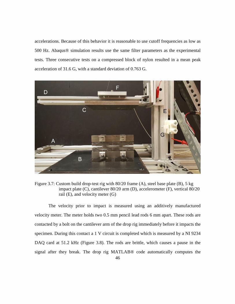
46
accelerations. Because of this behavior it is reasonable to use cutoff frequencies as low as
500 Hz. Abaqus® simulation results use the same filter parameters as the experimental
tests. Three consecutive tests on a compressed block of nylon resulted in a mean peak
acceleration of 31.6 G, with a standard deviation of 0.763 G.
Figure 3.7: Custom build drop-test rig with 80/20 frame (A), steel base plate (B), 5 kg
impact plate (C), cantilever 80/20 arm (D), accelerometer (F), vertical 80/20
rail (E), and velocity meter (G)
The velocity prior to impact is measured using an additively manufactured
velocity meter. The meter holds two 0.5 mm pencil lead rods 6 mm apart. These rods are
contacted by a bolt on the cantilever arm of the drop rig immediately before it impacts the
specimen. During this contact a 1 V circuit is completed which is measured by a NI 9234
DAQ card at 51.2 kHz (Figure 3.8). The rods are brittle, which causes a pause in the
signal after they break. The drop rig MATLAB® code automatically computes the
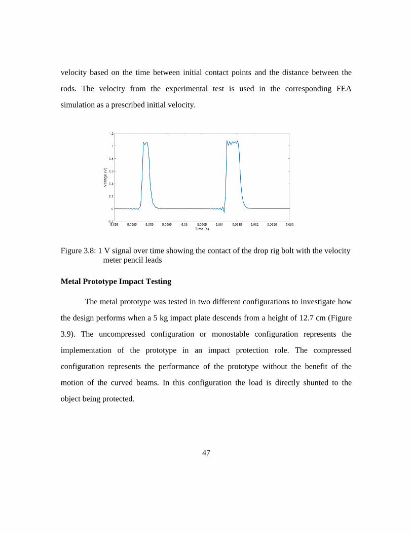
47
velocity based on the time between initial contact points and the distance between the
rods. The velocity from the experimental test is used in the corresponding FEA
simulation as a prescribed initial velocity.
Figure 3.8: 1 V signal over time showing the contact of the drop rig bolt with the velocity
meter pencil leads
Metal Prototype Impact Testing
The metal prototype was tested in two different configurations to investigate how
the design performs when a 5 kg impact plate descends from a height of 12.7 cm (Figure
3.9). The uncompressed configuration or monostable configuration represents the
implementation of the prototype in an impact protection role. The compressed
configuration represents the performance of the prototype without the benefit of the
motion of the curved beams. In this configuration the load is directly shunted to the
object being protected.
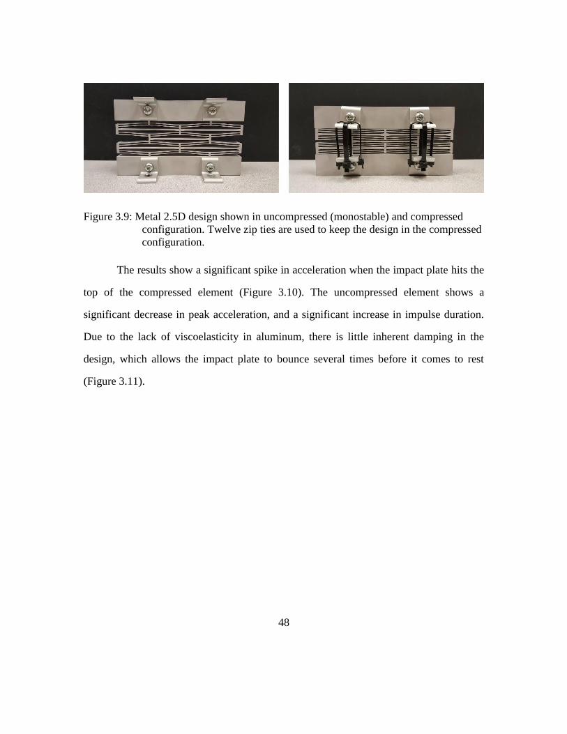
48
Figure 3.9: Metal 2.5D design shown in uncompressed (monostable) and compressed
configuration. Twelve zip ties are used to keep the design in the compressed
configuration.
The results show a significant spike in acceleration when the impact plate hits the
top of the compressed element (Figure 3.10). The uncompressed element shows a
significant decrease in peak acceleration, and a significant increase in impulse duration.
Due to the lack of viscoelasticity in aluminum, there is little inherent damping in the
design, which allows the impact plate to bounce several times before it comes to rest
(Figure 3.11).
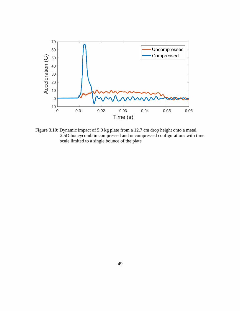
49
Figure 3.10: Dynamic impact of 5.0 kg plate from a 12.7 cm drop height onto a metal
2.5D honeycomb in compressed and uncompressed configurations with time
scale limited to a single bounce of the plate
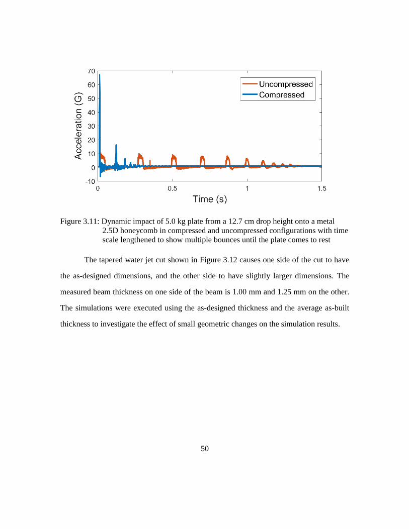
50
Figure 3.11: Dynamic impact of 5.0 kg plate from a 12.7 cm drop height onto a metal
2.5D honeycomb in compressed and uncompressed configurations with time
scale lengthened to show multiple bounces until the plate comes to rest
The tapered water jet cut shown in Figure 3.12 causes one side of the cut to have
the as-designed dimensions, and the other side to have slightly larger dimensions. The
measured beam thickness on one side of the beam is 1.00 mm and 1.25 mm on the other.
The simulations were executed using the as-designed thickness and the average as-built
thickness to investigate the effect of small geometric changes on the simulation results.
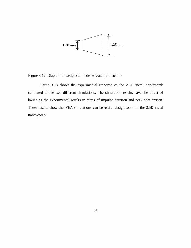
51
Figure 3.12: Diagram of wedge cut made by water jet machine
Figure 3.13 shows the experimental response of the 2.5D metal honeycomb
compared to the two different simulations. The simulation results have the effect of
bounding the experimental results in terms of impulse duration and peak acceleration.
These results show that FEA simulations can be useful design tools for the 2.5D metal
honeycomb.
1.00 mm 1.25 mm
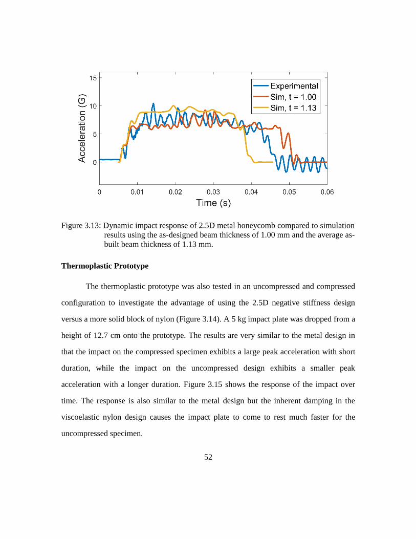
52
Figure 3.13: Dynamic impact response of 2.5D metal honeycomb compared to simulation
results using the as-designed beam thickness of 1.00 mm and the average as-
built beam thickness of 1.13 mm.
Thermoplastic Prototype
The thermoplastic prototype was also tested in an uncompressed and compressed
configuration to investigate the advantage of using the 2.5D negative stiffness design
versus a more solid block of nylon (Figure 3.14). A 5 kg impact plate was dropped from a
height of 12.7 cm onto the prototype. The results are very similar to the metal design in
that the impact on the compressed specimen exhibits a large peak acceleration with short
duration, while the impact on the uncompressed design exhibits a smaller peak
acceleration with a longer duration. Figure 3.15 shows the response of the impact over
time. The response is also similar to the metal design but the inherent damping in the
viscoelastic nylon design causes the impact plate to come to rest much faster for the
uncompressed specimen.
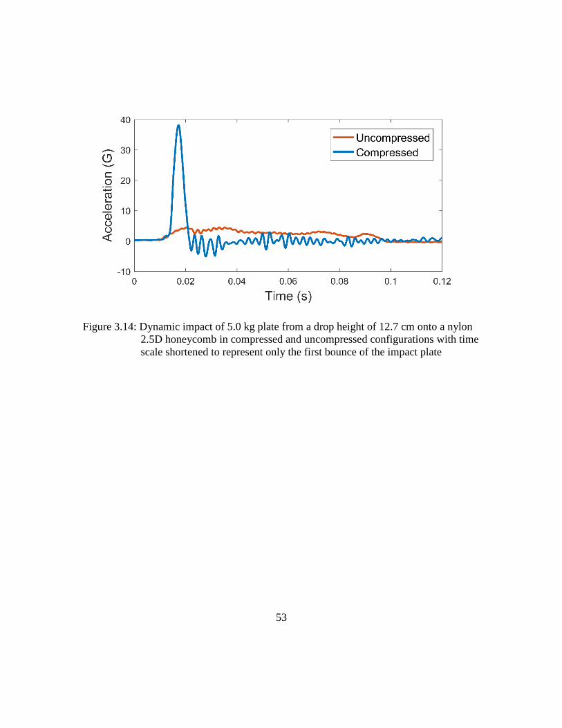
53
Figure 3.14: Dynamic impact of 5.0 kg plate from a drop height of 12.7 cm onto a nylon
2.5D honeycomb in compressed and uncompressed configurations with time
scale shortened to represent only the first bounce of the impact plate
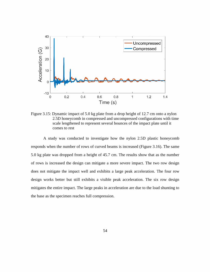
54
Figure 3.15: Dynamic impact of 5.0 kg plate from a drop height of 12.7 cm onto a nylon
2.5D honeycomb in compressed and uncompressed configurations with time
scale lengthened to represent several bounces of the impact plate until it
comes to rest
A study was conducted to investigate how the nylon 2.5D plastic honeycomb
responds when the number of rows of curved beams is increased (Figure 3.16). The same
5.0 kg plate was dropped from a height of 45.7 cm. The results show that as the number
of rows is increased the design can mitigate a more severe impact. The two row design
does not mitigate the impact well and exhibits a large peak acceleration. The four row
design works better but still exhibits a visible peak acceleration. The six row design
mitigates the entire impact. The large peaks in acceleration are due to the load shunting to
the base as the specimen reaches full compression.
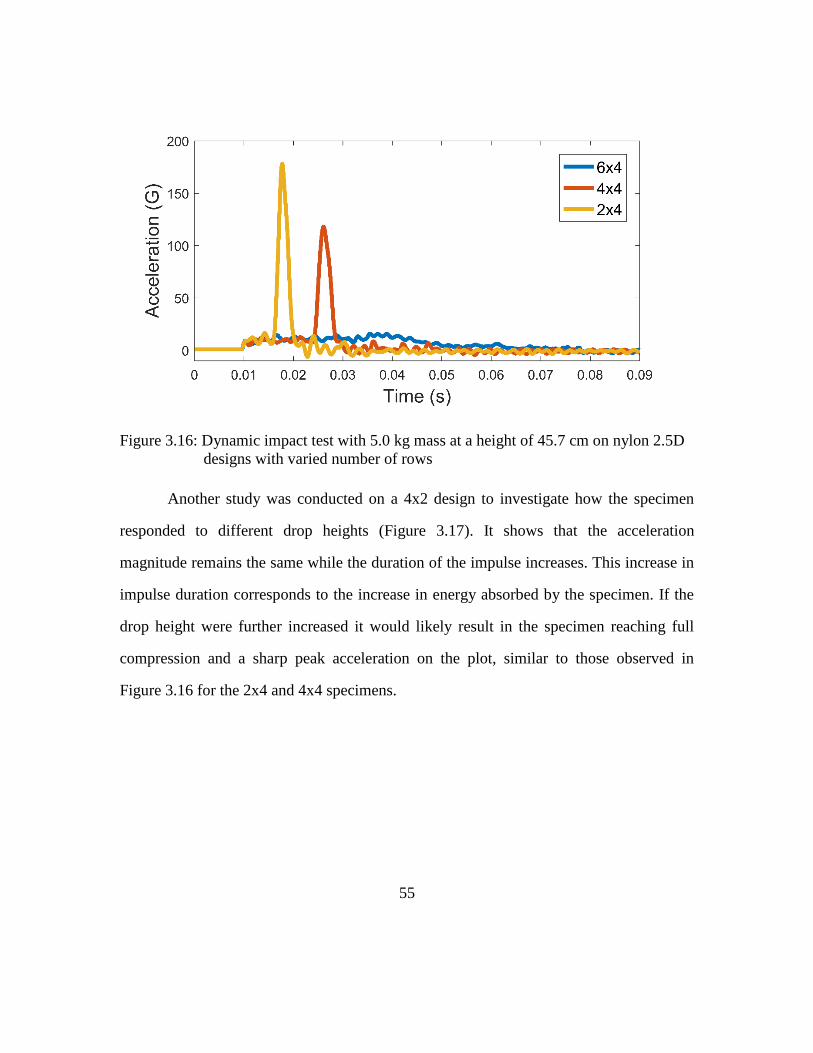
55
Figure 3.16: Dynamic impact test with 5.0 kg mass at a height of 45.7 cm on nylon 2.5D
designs with varied number of rows
Another study was conducted on a 4x2 design to investigate how the specimen
responded to different drop heights (Figure 3.17). It shows that the acceleration
magnitude remains the same while the duration of the impulse increases. This increase in
impulse duration corresponds to the increase in energy absorbed by the specimen. If the
drop height were further increased it would likely result in the specimen reaching full
compression and a sharp peak acceleration on the plot, similar to those observed in
Figure 3.16 for the 2x4 and 4x4 specimens.
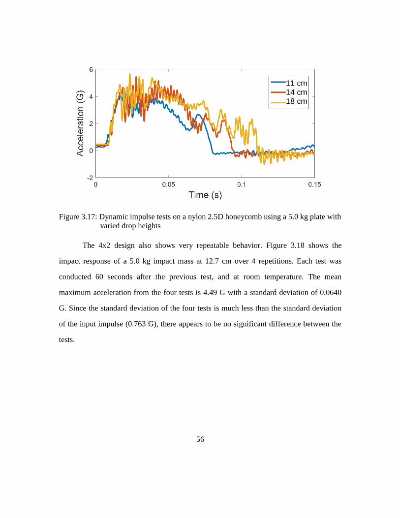
56
Figure 3.17: Dynamic impulse tests on a nylon 2.5D honeycomb using a 5.0 kg plate with
varied drop heights
The 4x2 design also shows very repeatable behavior. Figure 3.18 shows the
impact response of a 5.0 kg impact mass at 12.7 cm over 4 repetitions. Each test was
conducted 60 seconds after the previous test, and at room temperature. The mean
maximum acceleration from the four tests is 4.49 G with a standard deviation of 0.0640
G. Since the standard deviation of the four tests is much less than the standard deviation
of the input impulse (0.763 G), there appears to be no significant difference between the
tests.
11 cm 14 cm 18 cm
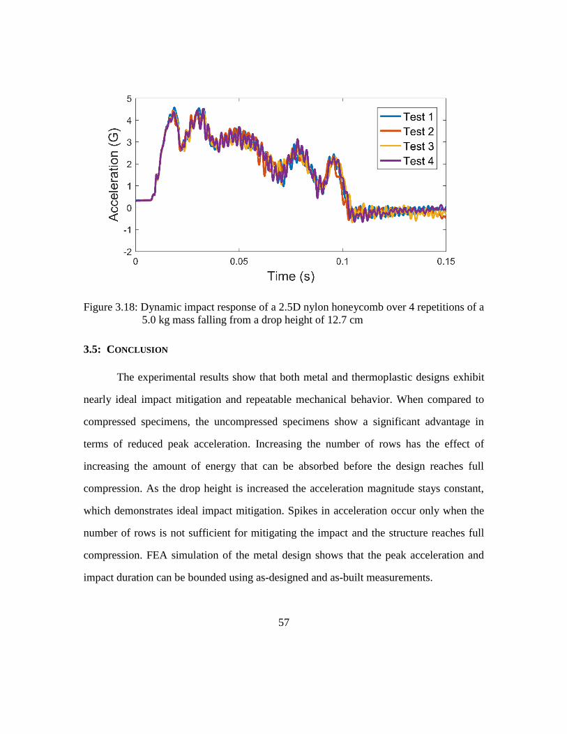
57
Figure 3.18: Dynamic impact response of a 2.5D nylon honeycomb over 4 repetitions of a
5.0 kg mass falling from a drop height of 12.7 cm
3.5: CONCLUSION
The experimental results show that both metal and thermoplastic designs exhibit
nearly ideal impact mitigation and repeatable mechanical behavior. When compared to
compressed specimens, the uncompressed specimens show a significant advantage in
terms of reduced peak acceleration. Increasing the number of rows has the effect of
increasing the amount of energy that can be absorbed before the design reaches full
compression. As the drop height is increased the acceleration magnitude stays constant,
which demonstrates ideal impact mitigation. Spikes in acceleration occur only when the
number of rows is not sufficient for mitigating the impact and the structure reaches full
compression. FEA simulation of the metal design shows that the peak acceleration and
impact duration can be bounded using as-designed and as-built measurements.
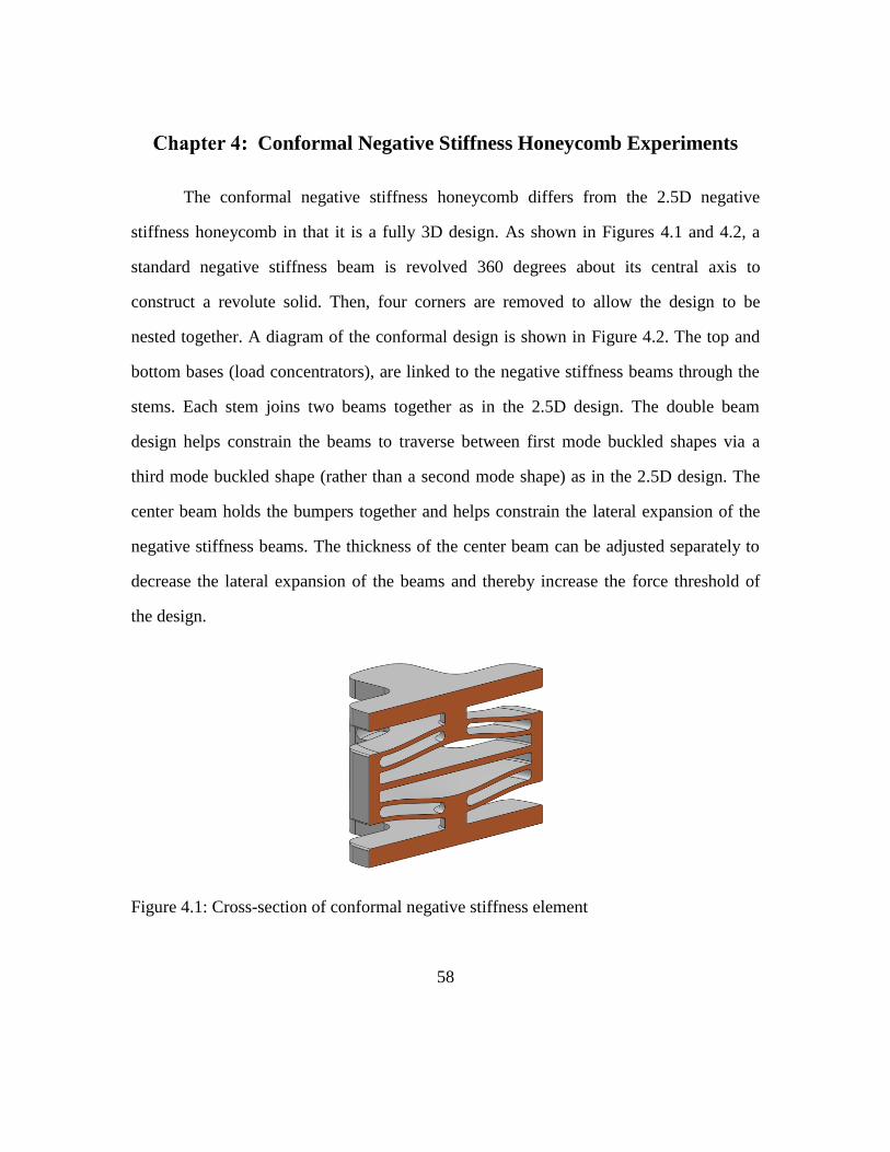
58
Conformal Negative Stiffness Honeycomb Experiments
The conformal negative stiffness honeycomb differs from the 2.5D negative
stiffness honeycomb in that it is a fully 3D design. As shown in Figures 4.1 and 4.2, a
standard negative stiffness beam is revolved 360 degrees about its central axis to
construct a revolute solid. Then, four corners are removed to allow the design to be
nested together. A diagram of the conformal design is shown in Figure 4.2. The top and
bottom bases (load concentrators), are linked to the negative stiffness beams through the
stems. Each stem joins two beams together as in the 2.5D design. The double beam
design helps constrain the beams to traverse between first mode buckled shapes via a
third mode buckled shape (rather than a second mode shape) as in the 2.5D design. The
center beam holds the bumpers together and helps constrain the lateral expansion of the
negative stiffness beams. The thickness of the center beam can be adjusted separately to
decrease the lateral expansion of the beams and thereby increase the force threshold of
the design.
Figure 4.1: Cross-section of conformal negative stiffness element
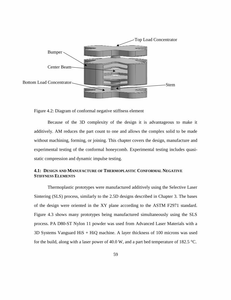
59
Figure 4.2: Diagram of conformal negative stiffness element
Because of the 3D complexity of the design it is advantageous to make it
additively. AM reduces the part count to one and allows the complex solid to be made
without machining, forming, or joining. This chapter covers the design, manufacture and
experimental testing of the conformal honeycomb. Experimental testing includes quasi-
static compression and dynamic impulse testing.
4.1: DESIGN AND MANUFACTURE OF THERMOPLASTIC CONFORMAL NEGATIVE
STIFFNESS ELEMENTS
Thermoplastic prototypes were manufactured additively using the Selective Laser
Sintering (SLS) process, similarly to the 2.5D designs described in Chapter 3. The bases
of the design were oriented in the XY plane according to the ASTM F2971 standard.
Figure 4.3 shows many prototypes being manufactured simultaneously using the SLS
process. PA D80-ST Nylon 11 powder was used from Advanced Laser Materials with a
3D Systems Vanguard HiS + HiQ machine. A layer thickness of 100 microns was used
for the build, along with a laser power of 40.0 W, and a part bed temperature of 182.5 °C.
Bumper
Center Beam
Bottom Load Concentrator
Top Load Concentrator
Stem
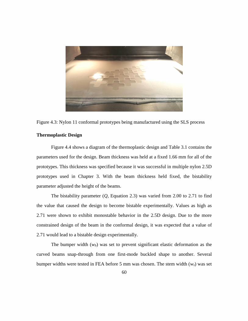
60
Figure 4.3: Nylon 11 conformal prototypes being manufactured using the SLS process
Thermoplastic Design
Figure 4.4 shows a diagram of the thermoplastic design and Table 3.1 contains the
parameters used for the design. Beam thickness was held at a fixed 1.66 mm for all of the
prototypes. This thickness was specified because it was successful in multiple nylon 2.5D
prototypes used in Chapter 3. With the beam thickness held fixed, the bistability
parameter adjusted the height of the beams.
The bistability parameter (Q, Equation 2.3) was varied from 2.00 to 2.71 to find
the value that caused the design to become bistable experimentally. Values as high as
2.71 were shown to exhibit monostable behavior in the 2.5D design. Due to the more
constrained design of the beam in the conformal design, it was expected that a value of
2.71 would lead to a bistable design experimentally.
The bumper width (wb) was set to prevent significant elastic deformation as the
curved beams snap-through from one first-mode buckled shape to another. Several
bumper widths were tested in FEA before 5 mm was chosen. The stem width (ws) was set
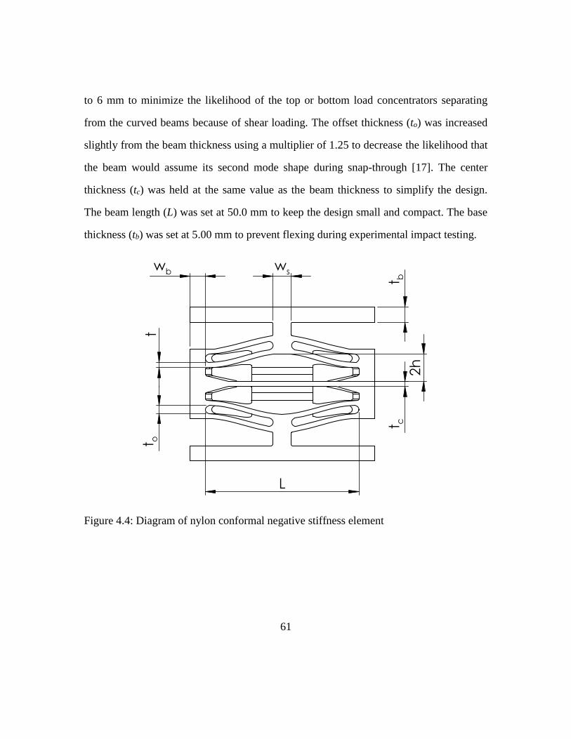
61
to 6 mm to minimize the likelihood of the top or bottom load concentrators separating
from the curved beams because of shear loading. The offset thickness (to) was increased
slightly from the beam thickness using a multiplier of 1.25 to decrease the likelihood that
the beam would assume its second mode shape during snap-through [17]. The center
thickness (tc) was held at the same value as the beam thickness to simplify the design.
The beam length (L) was set at 50.0 mm to keep the design small and compact. The base
thickness (tb) was set at 5.00 mm to prevent flexing during experimental impact testing.
Figure 4.4: Diagram of nylon conformal negative stiffness element
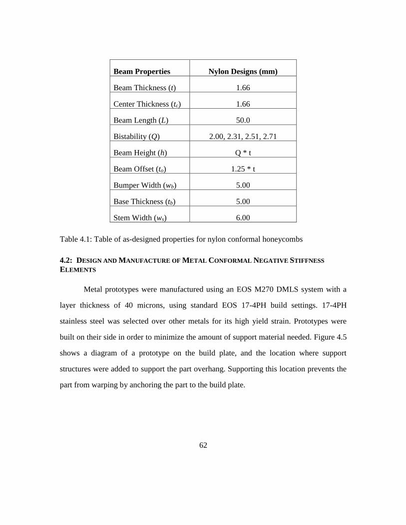
62
Beam Properties Nylon Designs (mm)
Beam Thickness (t) 1.66
Center Thickness (tc) 1.66
Beam Length (L) 50.0
Bistability (Q) 2.00, 2.31, 2.51, 2.71
Beam Height (h) Q * t
Beam Offset (to) 1.25 * t
Bumper Width (wb) 5.00
Base Thickness (tb) 5.00
Stem Width (ws) 6.00
Table 4.1: Table of as-designed properties for nylon conformal honeycombs
4.2: DESIGN AND MANUFACTURE OF METAL CONFORMAL NEGATIVE STIFFNESS
ELEMENTS
Metal prototypes were manufactured using an EOS M270 DMLS system with a
layer thickness of 40 microns, using standard EOS 17-4PH build settings. 17-4PH
stainless steel was selected over other metals for its high yield strain. Prototypes were
built on their side in order to minimize the amount of support material needed. Figure 4.5
shows a diagram of a prototype on the build plate, and the location where support
structures were added to support the part overhang. Supporting this location prevents the
part from warping by anchoring the part to the build plate.
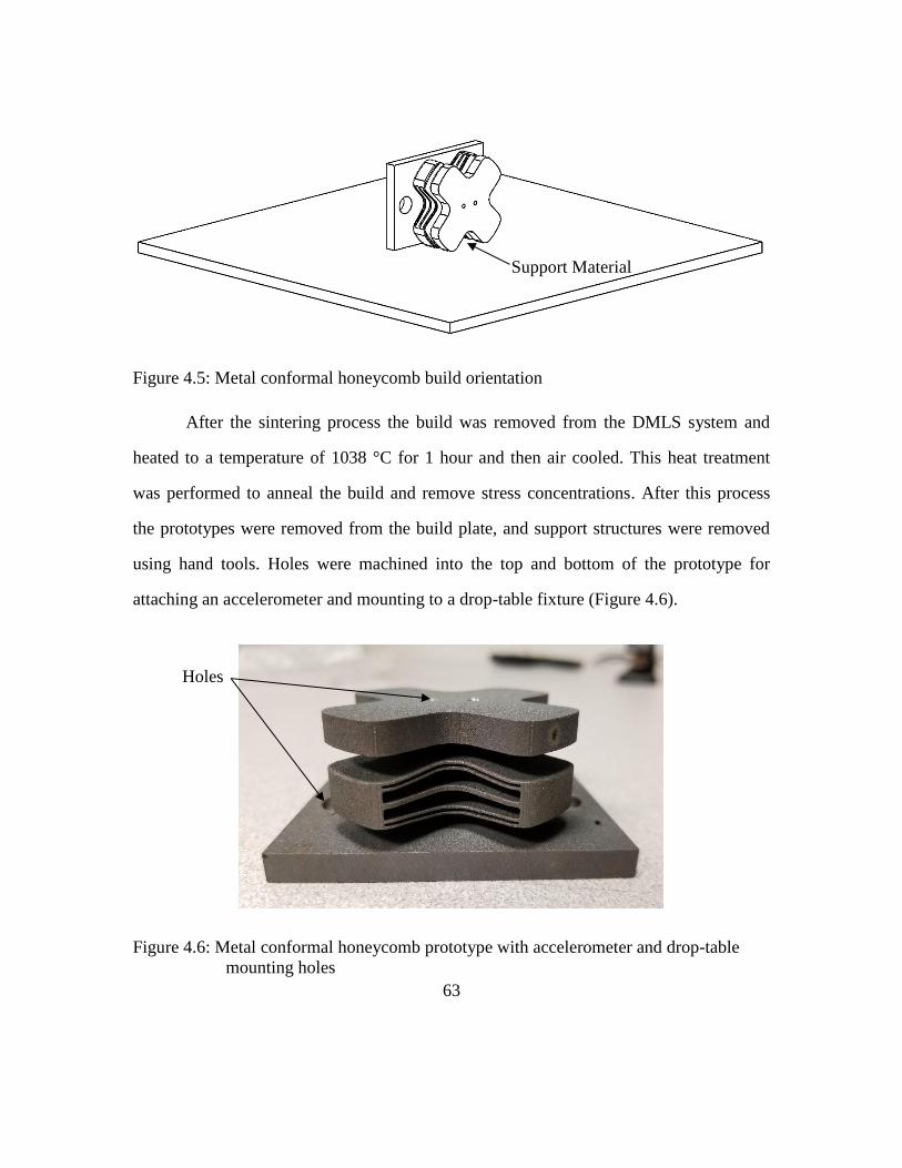
63
Figure 4.5: Metal conformal honeycomb build orientation
After the sintering process the build was removed from the DMLS system and
heated to a temperature of 1038 °C for 1 hour and then air cooled. This heat treatment
was performed to anneal the build and remove stress concentrations. After this process
the prototypes were removed from the build plate, and support structures were removed
using hand tools. Holes were machined into the top and bottom of the prototype for
attaching an accelerometer and mounting to a drop-table fixture (Figure 4.6).
Figure 4.6: Metal conformal honeycomb prototype with accelerometer and drop-table
mounting holes
Support Material
Holes
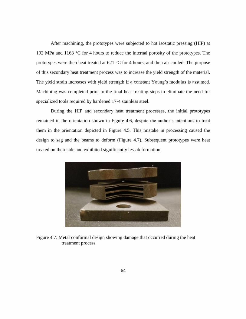
64
After machining, the prototypes were subjected to hot isostatic pressing (HIP) at
102 MPa and 1163 °C for 4 hours to reduce the internal porosity of the prototypes. The
prototypes were then heat treated at 621 °C for 4 hours, and then air cooled. The purpose
of this secondary heat treatment process was to increase the yield strength of the material.
The yield strain increases with yield strength if a constant Young’s modulus is assumed.
Machining was completed prior to the final heat treating steps to eliminate the need for
specialized tools required by hardened 17-4 stainless steel.
During the HIP and secondary heat treatment processes, the initial prototypes
remained in the orientation shown in Figure 4.6, despite the author’s intentions to treat
them in the orientation depicted in Figure 4.5. This mistake in processing caused the
design to sag and the beams to deform (Figure 4.7). Subsequent prototypes were heat
treated on their side and exhibited significantly less deformation.
Figure 4.7: Metal conformal design showing damage that occurred during the heat
treatment process
65
Metal Design
Figure 4.8 shows a diagram of the metal conformal honeycomb and Table 4.3
documents the associated design parameters. A beam thickness of 0.50 mm was used for
the metal conformal design because it was the smallest feature size recommended by the
manufacturer. The beam thickness (t) was minimized in order to maximize the apex
height (h) of the curved beams and therefore maximize the force threshold without
exceeding the yield strain of the material, as guided by the yield strain equation (Equation
2.6). Material property data was supplied by the manufacturer (Table 4.2). A safety factor
(sf) of 1.11 was applied to the yield strength (y) before calculating the yield strain
(Equation 4.1) to reduce the likelihood of plastic deformation in the beams.
𝜀𝑚𝑎𝑥 = log(1 +𝑠𝑓∗𝑦
𝐸+ 0.002) (4.1)
The beam length (L) was maximized but limited so that the beams would not
interfere with mounting holes on the drop-table for impact testing. Greater beam lengths
allow greater beam heights according to the yield strain equation (Equation 2.6). The
center thickness (tc) was specified as double the beam thickness to make the later
constraints more rigid and increase the force threshold. The bumper width (wb) was
minimized to reduce mass and decrease the chance that the bottom row would snap-
through under a severe impulse before the top row. FEA trials limited the minimum
bumper width to avoid significant flexing of the bumper as the curved beams snapped-
through from one first-mode buckled shape, which is important for maximizing the force
threshold. The base thickness (tb) was set at 5.00 mm to add mass to the top of the
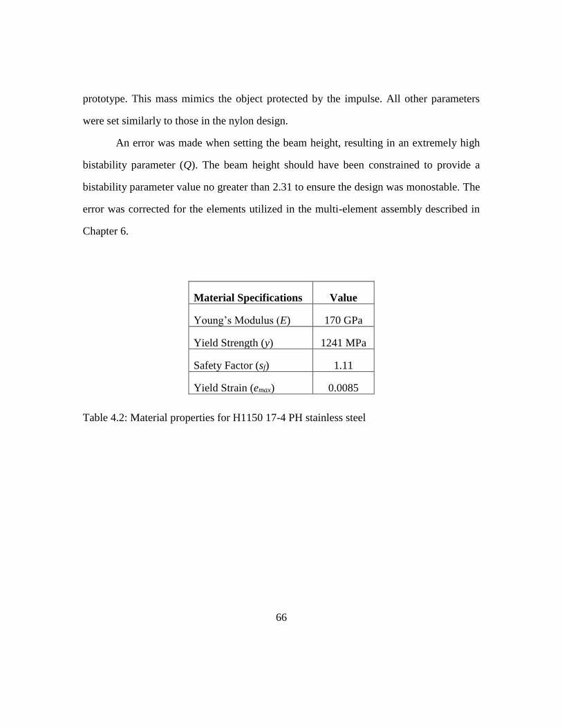
66
prototype. This mass mimics the object protected by the impulse. All other parameters
were set similarly to those in the nylon design.
An error was made when setting the beam height, resulting in an extremely high
bistability parameter (Q). The beam height should have been constrained to provide a
bistability parameter value no greater than 2.31 to ensure the design was monostable. The
error was corrected for the elements utilized in the multi-element assembly described in
Chapter 6.
Material Specifications Value
Young’s Modulus (E) 170 GPa
Yield Strength (y) 1241 MPa
Safety Factor (sf) 1.11
Yield Strain (emax) 0.0085
Table 4.2: Material properties for H1150 17-4 PH stainless steel
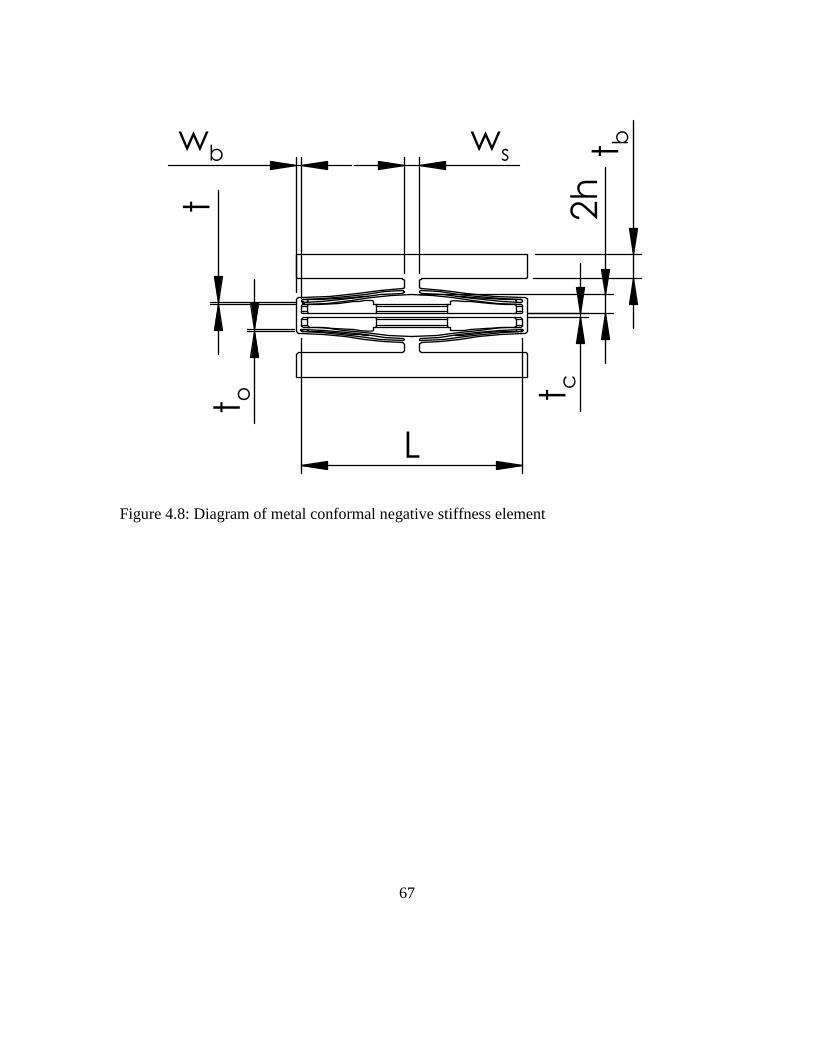
67
Figure 4.8: Diagram of metal conformal negative stiffness element
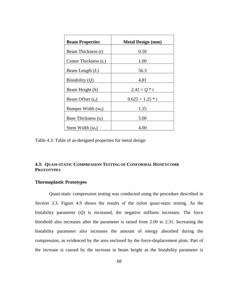
68
Beam Properties Metal Design (mm)
Beam Thickness (t) 0.50
Center Thickness (tc) 1.00
Beam Length (L) 56.3
Bistability (Q) 4.81
Beam Height (h) 2.41 = Q * t
Beam Offset (to) 0.625 = 1.25 * t
Bumper Width (wb) 1.25
Base Thickness (tb) 5.00
Stem Width (ws) 4.00
Table 4.3: Table of as-designed properties for metal design
4.3: QUASI-STATIC COMPRESSION TESTING OF CONFORMAL HONEYCOMB
PROTOTYPES
Thermoplastic Prototypes
Quasi-static compression testing was conducted using the procedure described in
Section 3.3. Figure 4.9 shows the results of the nylon quasi-static testing. As the
bistability parameter (Q) is increased, the negative stiffness increases. The force
threshold also increases after the parameter is raised from 2.00 to 2.31. Increasing the
bistability parameter also increases the amount of energy absorbed during the
compression, as evidenced by the area enclosed by the force-displacement plots. Part of
the increase is caused by the increase in beam height as the bistability parameter is
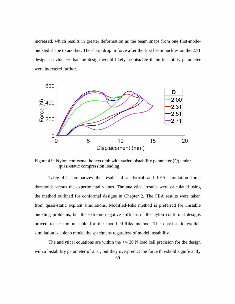
69
increased, which results in greater deformation as the beam snaps from one first-mode-
buckled shape to another. The sharp drop in force after the first beam buckles on the 2.71
design is evidence that the design would likely be bistable if the bistability parameter
were increased further.
Figure 4.9: Nylon conformal honeycomb with varied bistability parameter (Q) under
quasi-static compression loading
Table 4.4 summarizes the results of analytical and FEA simulation force
thresholds versus the experimental values. The analytical results were calculated using
the method outlined for conformal designs in Chapter 2. The FEA results were taken
from quasi-static explicit simulations. Modified-Riks method is preferred for unstable
buckling problems, but the extreme negative stiffness of the nylon conformal designs
proved to be too unstable for the modified-Riks method. The quasi-static explicit
simulation is able to model the specimens regardless of model instability.
The analytical equations are within the +/- 20 N load cell precision for the design
with a bistability parameter of 2.51, but they overpredict the force threshold significantly
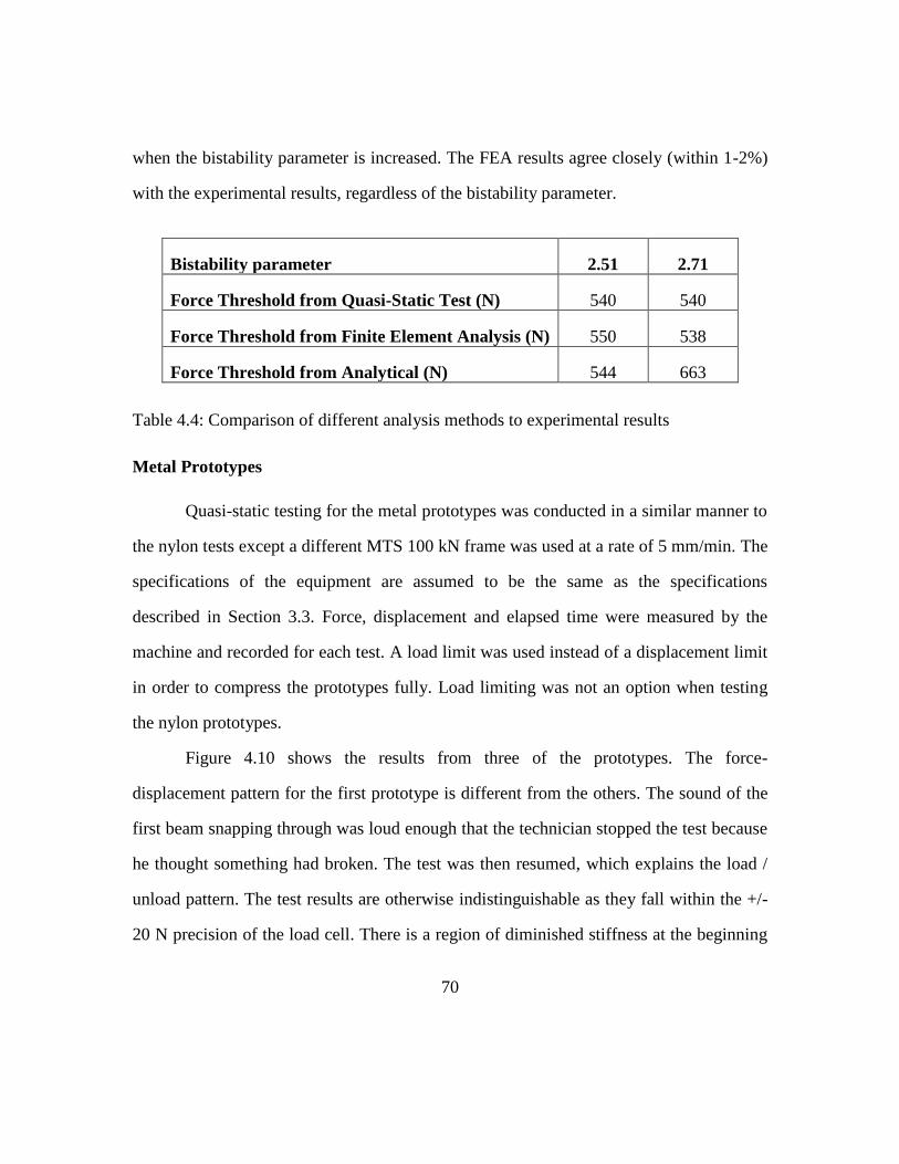
70
when the bistability parameter is increased. The FEA results agree closely (within 1-2%)
with the experimental results, regardless of the bistability parameter.
Bistability parameter 2.51 2.71
Force Threshold from Quasi-Static Test (N) 540 540
Force Threshold from Finite Element Analysis (N) 550 538
Force Threshold from Analytical (N) 544 663
Table 4.4: Comparison of different analysis methods to experimental results
Metal Prototypes
Quasi-static testing for the metal prototypes was conducted in a similar manner to
the nylon tests except a different MTS 100 kN frame was used at a rate of 5 mm/min. The
specifications of the equipment are assumed to be the same as the specifications
described in Section 3.3. Force, displacement and elapsed time were measured by the
machine and recorded for each test. A load limit was used instead of a displacement limit
in order to compress the prototypes fully. Load limiting was not an option when testing
the nylon prototypes.
Figure 4.10 shows the results from three of the prototypes. The force-
displacement pattern for the first prototype is different from the others. The sound of the
first beam snapping through was loud enough that the technician stopped the test because
he thought something had broken. The test was then resumed, which explains the load /
unload pattern. The test results are otherwise indistinguishable as they fall within the +/-
20 N precision of the load cell. There is a region of diminished stiffness at the beginning
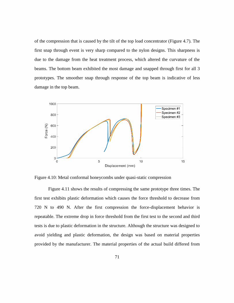
71
of the compression that is caused by the tilt of the top load concentrator (Figure 4.7). The
first snap through event is very sharp compared to the nylon designs. This sharpness is
due to the damage from the heat treatment process, which altered the curvature of the
beams. The bottom beam exhibited the most damage and snapped through first for all 3
prototypes. The smoother snap through response of the top beam is indicative of less
damage in the top beam.
Figure 4.10: Metal conformal honeycombs under quasi-static compression
Figure 4.11 shows the results of compressing the same prototype three times. The
first test exhibits plastic deformation which causes the force threshold to decrease from
720 N to 490 N. After the first compression the force-displacement behavior is
repeatable. The extreme drop in force threshold from the first test to the second and third
tests is due to plastic deformation in the structure. Although the structure was designed to
avoid yielding and plastic deformation, the design was based on material properties
provided by the manufacturer. The material properties of the actual build differed from
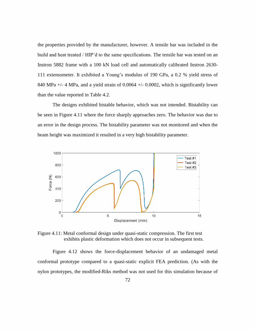
72
the properties provided by the manufacturer, however. A tensile bar was included in the
build and heat treated / HIP’d to the same specifications. The tensile bar was tested on an
Instron 5882 frame with a 100 kN load cell and automatically calibrated Instron 2630-
111 extensometer. It exhibited a Young’s modulus of 190 GPa, a 0.2 % yield stress of
840 MPa +/- 4 MPa, and a yield strain of 0.0064 +/- 0.0002, which is significantly lower
than the value reported in Table 4.2.
The designs exhibited bistable behavior, which was not intended. Bistability can
be seen in Figure 4.11 where the force sharply approaches zero. The behavior was due to
an error in the design process. The bistability parameter was not monitored and when the
beam height was maximized it resulted in a very high bistability parameter.
Figure 4.11: Metal conformal design under quasi-static compression. The first test
exhibits plastic deformation which does not occur in subsequent tests.
Figure 4.12 shows the force-displacement behavior of an undamaged metal
conformal prototype compared to a quasi-static explicit FEA prediction. (As with the
nylon prototypes, the modified-Riks method was not used for this simulation because of
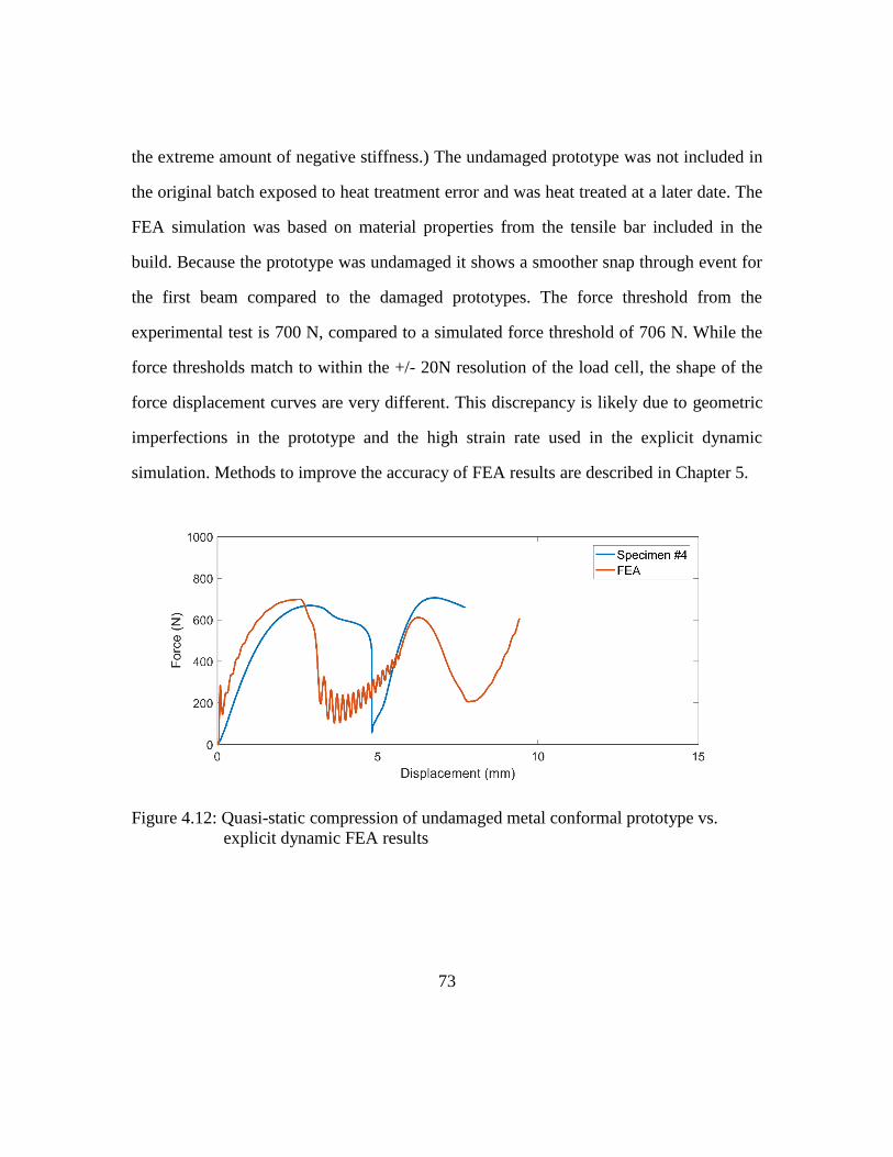
73
the extreme amount of negative stiffness.) The undamaged prototype was not included in
the original batch exposed to heat treatment error and was heat treated at a later date. The
FEA simulation was based on material properties from the tensile bar included in the
build. Because the prototype was undamaged it shows a smoother snap through event for
the first beam compared to the damaged prototypes. The force threshold from the
experimental test is 700 N, compared to a simulated force threshold of 706 N. While the
force thresholds match to within the +/- 20N resolution of the load cell, the shape of the
force displacement curves are very different. This discrepancy is likely due to geometric
imperfections in the prototype and the high strain rate used in the explicit dynamic
simulation. Methods to improve the accuracy of FEA results are described in Chapter 5.
Figure 4.12: Quasi-static compression of undamaged metal conformal prototype vs.
explicit dynamic FEA results
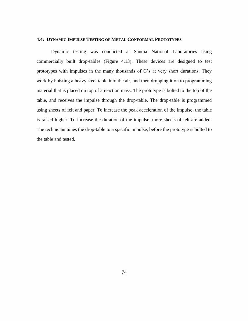
74
4.4: DYNAMIC IMPULSE TESTING OF METAL CONFORMAL PROTOTYPES
Dynamic testing was conducted at Sandia National Laboratories using
commercially built drop-tables (Figure 4.13). These devices are designed to test
prototypes with impulses in the many thousands of G’s at very short durations. They
work by hoisting a heavy steel table into the air, and then dropping it on to programming
material that is placed on top of a reaction mass. The prototype is bolted to the top of the
table, and receives the impulse through the drop-table. The drop-table is programmed
using sheets of felt and paper. To increase the peak acceleration of the impulse, the table
is raised higher. To increase the duration of the impulse, more sheets of felt are added.
The technician tunes the drop-table to a specific impulse, before the prototype is bolted to
the table and tested.
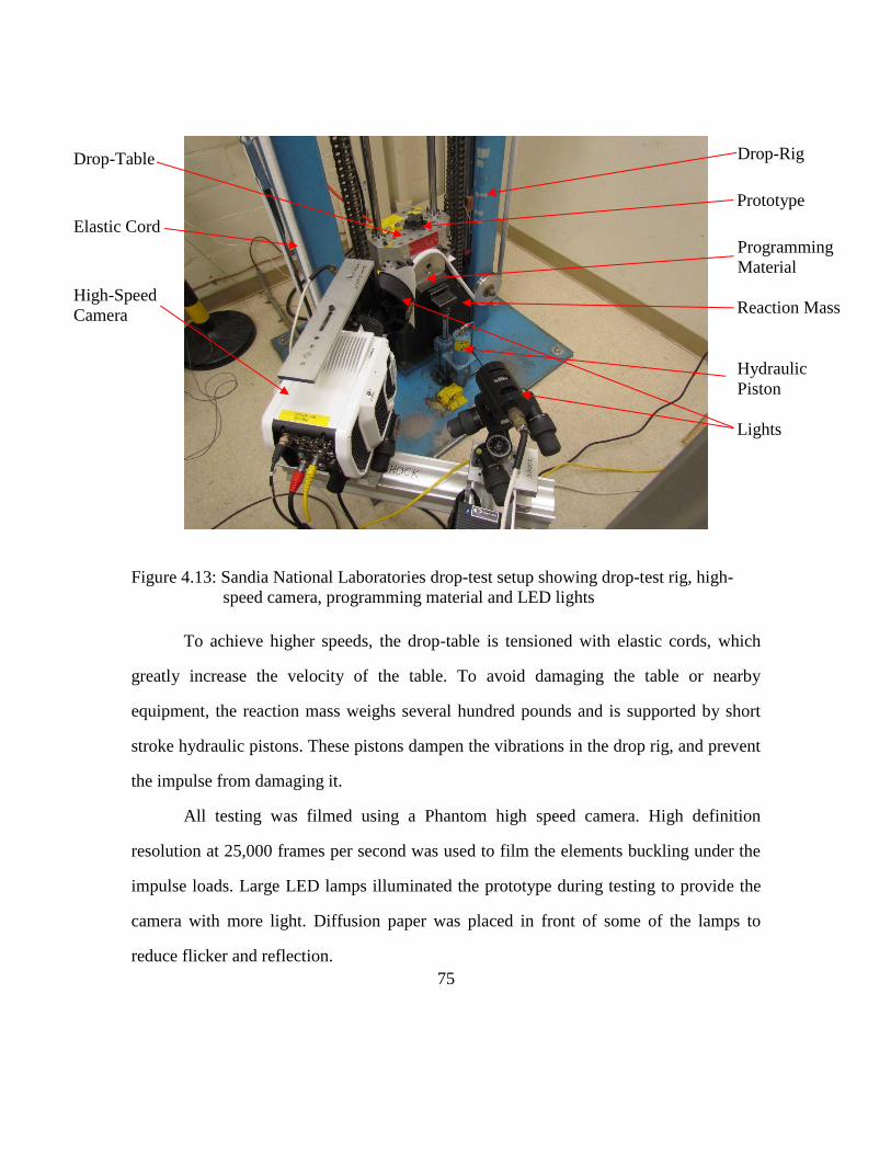
75
Figure 4.13: Sandia National Laboratories drop-test setup showing drop-test rig, high-
speed camera, programming material and LED lights
To achieve higher speeds, the drop-table is tensioned with elastic cords, which
greatly increase the velocity of the table. To avoid damaging the table or nearby
equipment, the reaction mass weighs several hundred pounds and is supported by short
stroke hydraulic pistons. These pistons dampen the vibrations in the drop rig, and prevent
the impulse from damaging it.
All testing was filmed using a Phantom high speed camera. High definition
resolution at 25,000 frames per second was used to film the elements buckling under the
impulse loads. Large LED lamps illuminated the prototype during testing to provide the
camera with more light. Diffusion paper was placed in front of some of the lamps to
reduce flicker and reflection.
High-Speed
Camera
Lights
Drop-Rig
Programming
Material
Prototype
Reaction Mass
Hydraulic
Piston
Drop-Table
Elastic Cord
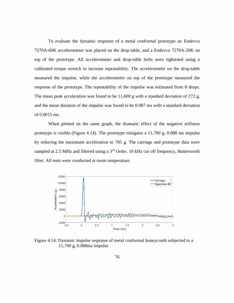
76
To evaluate the dynamic response of a metal conformal prototype an Endevco
7270A-60K accelerometer was placed on the drop-table, and a Endevco 7270A-20K on
top of the prototype. All accelerometer and drop-table bolts were tightened using a
calibrated torque wrench to increase repeatability. The accelerometer on the drop-table
measured the impulse, while the accelerometer on top of the prototype measured the
response of the prototype. The repeatability of the impulse was estimated from 8 drops.
The mean peak acceleration was found to be 11,600 g with a standard deviation of 272 g,
and the mean duration of the impulse was found to be 0.087 ms with a standard deviation
of 0.0015 ms.
When plotted on the same graph, the dramatic effect of the negative stiffness
prototype is visible (Figure 4.14). The prototype mitigates a 11,700 g, 0.088 ms impulse
by reducing the maximum acceleration to 785 g. The carriage and prototype data were
sampled at 2.5 MHz and filtered using a 3rd Order, 10 kHz cut off frequency, Butterworth
filter. All tests were conducted at room temperature.
Figure 4.14: Dynamic impulse response of metal conformal honeycomb subjected to a
11,700 g, 0.088ms impulse
77
Figure 4.15 shows the results of sequential tests with the same impulse. The mean
maximum acceleration from the two tests is 832 g with a standard deviation of 66.8 g.
Since the standard deviation between the two tests is much less than the standard
deviation of the input impulse (272 g), there appears to be no significant difference.
Figure 4.15: Repeated dynamic impulse tests of a single conformal metal honeycomb
showing the repeatability of its mechanical impulse response
The experimental response is compared to dynamic explicit simulation results in
Figure 4.16. Both sets of results were filtered using a 3rd Order, 10 kHz cut off frequency,
Butterworth filter. The results show that the maximum acceleration of the simulation
(758 g), falls within one standard deviation of the experimental result (785 g). There is
therefore no significant difference between the maximum accelerations.
The time domain does not match well, however. Some of the discrepancies may
be attributed to the plastic deformation experienced by the physical prototype prior to
dynamic impulse testing. The procedures for simulating multiple compressions had not
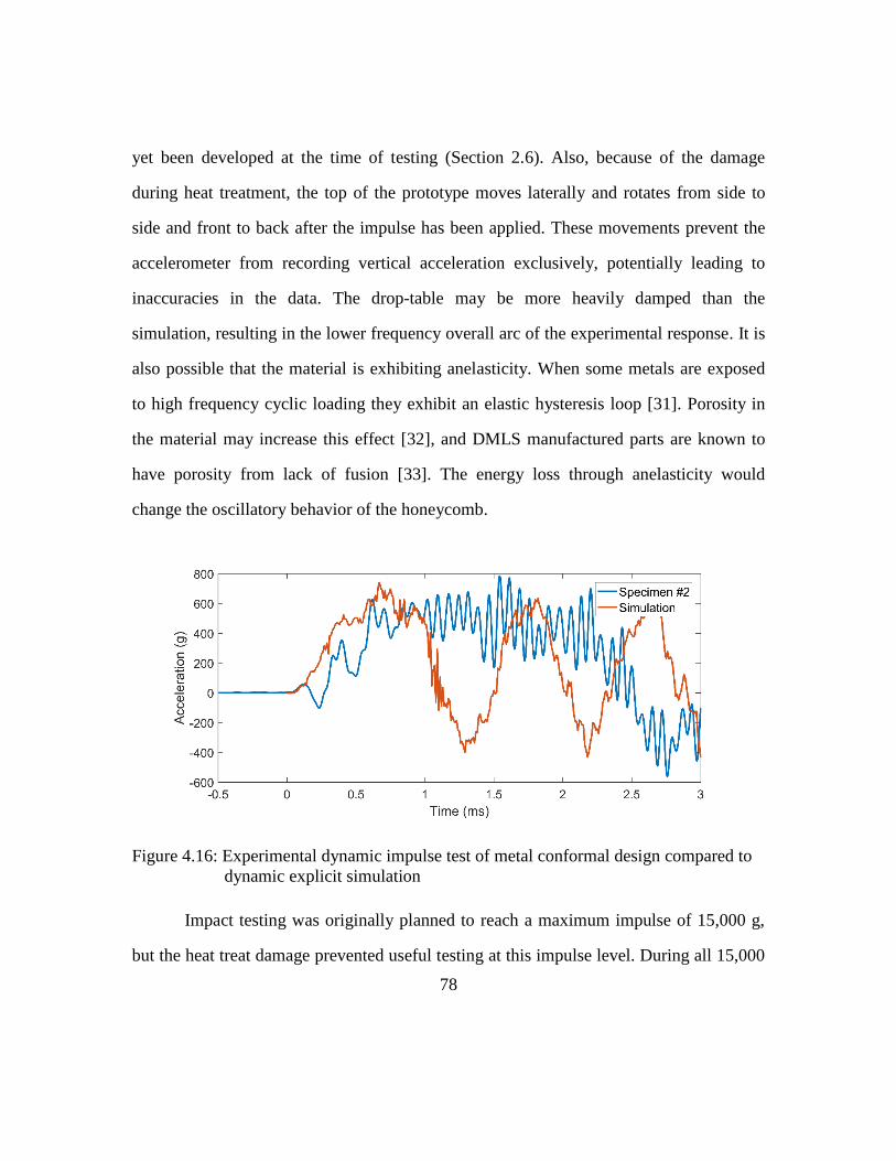
78
yet been developed at the time of testing (Section 2.6). Also, because of the damage
during heat treatment, the top of the prototype moves laterally and rotates from side to
side and front to back after the impulse has been applied. These movements prevent the
accelerometer from recording vertical acceleration exclusively, potentially leading to
inaccuracies in the data. The drop-table may be more heavily damped than the
simulation, resulting in the lower frequency overall arc of the experimental response. It is
also possible that the material is exhibiting anelasticity. When some metals are exposed
to high frequency cyclic loading they exhibit an elastic hysteresis loop [31]. Porosity in
the material may increase this effect [32], and DMLS manufactured parts are known to
have porosity from lack of fusion [33]. The energy loss through anelasticity would
change the oscillatory behavior of the honeycomb.
Figure 4.16: Experimental dynamic impulse test of metal conformal design compared to
dynamic explicit simulation
Impact testing was originally planned to reach a maximum impulse of 15,000 g,
but the heat treat damage prevented useful testing at this impulse level. During all 15,000
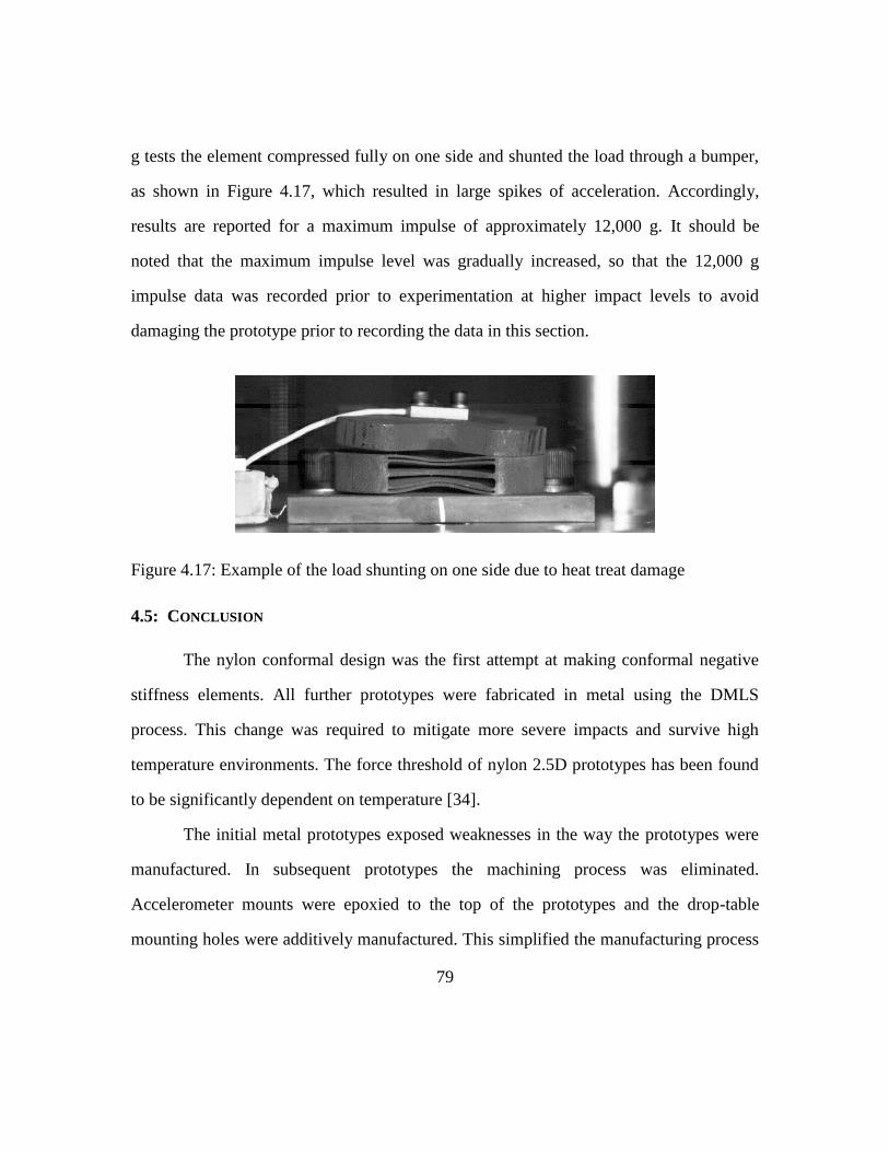
79
g tests the element compressed fully on one side and shunted the load through a bumper,
as shown in Figure 4.17, which resulted in large spikes of acceleration. Accordingly,
results are reported for a maximum impulse of approximately 12,000 g. It should be
noted that the maximum impulse level was gradually increased, so that the 12,000 g
impulse data was recorded prior to experimentation at higher impact levels to avoid
damaging the prototype prior to recording the data in this section.
Figure 4.17: Example of the load shunting on one side due to heat treat damage
4.5: CONCLUSION
The nylon conformal design was the first attempt at making conformal negative
stiffness elements. All further prototypes were fabricated in metal using the DMLS
process. This change was required to mitigate more severe impacts and survive high
temperature environments. The force threshold of nylon 2.5D prototypes has been found
to be significantly dependent on temperature [34].
The initial metal prototypes exposed weaknesses in the way the prototypes were
manufactured. In subsequent prototypes the machining process was eliminated.
Accelerometer mounts were epoxied to the top of the prototypes and the drop-table
mounting holes were additively manufactured. This simplified the manufacturing process
80
and allowed the prototypes to remain on the build plate during heat treatment, which
prevented the possibility of the prototypes being heat treated in the wrong orientation.
Prototypes were also cut off of the build plate using a wire EDM machine in order to
minimize the potential for damage caused by a band saw, which is the standard method
for removing parts from the build plate.
The tests also exposed weaknesses in the design and simulation of the prototypes.
It is hypothesized that differences between as-designed and as-built geometries and
material properties, combined with plastic deformation during the first load-unload cycle
of the metallic conformal honeycombs, resulted in discrepancies between experimental
results and simulation-based predictions of force-displacement behavior. The need for a
way of incorporating sources of variability in geometry and material properties into the
design process became apparent. A method for doing this is discussed in the next chapter.
81
Predictability and Reliability Modeling
Modeling performance variability is an important step in the product design
process. It is exceptionally important in additive manufacturing (AM) applications, which
are often associated with high levels of geometric and material property variability. For
this chapter the performance space of an example design will be explored. The
performance variable will be force threshold, or the force required to transition a negative
stiffness beam from one first mode buckled geometry to another. The chapter will begin
with a discussion on the challenges associated with using AM, and transition to an
explanation of the sources of variability that affect part performance. Beam shape
imperfections in a manufactured sample will be identified using computed tomography
(CT), and a pipeline will be created to map imperfections to finite element models. Then,
an uncertainty analysis will be conducted that takes into account variability in material
properties, beam thickness, beam height, and geometric shape. The predictions will then
be compared to experimental results.
5.1 PREDICTABILITY OF MECHANICAL BEHAVIOR OF DIRECT METAL LASER
SINTERED PARTS
Direct Metal Laser Sintering (DMLS), also called Selective Laser Melting (SLM),
is a common metal additive manufacturing method commercialized by EOS GmbH and
other companies [35]. Compared to metal subtractive manufacturing, DMLS provides
designers with the freedom to build parts with complex topologies. Such parts may be
extremely expensive or even impossible to manufacture conventionally.
The process is similar to the Selective Laser Sintering (SLS) method used for
producing plastic parts in that a powdered material is melted using a laser, and new layers
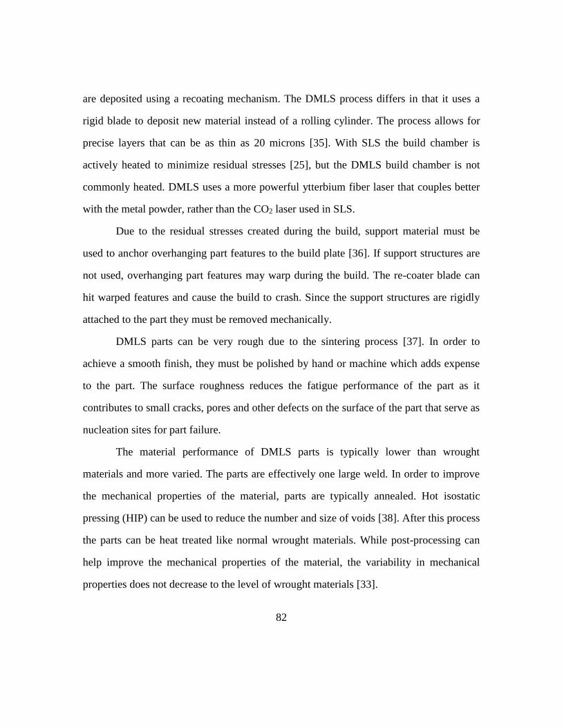
82
are deposited using a recoating mechanism. The DMLS process differs in that it uses a
rigid blade to deposit new material instead of a rolling cylinder. The process allows for
precise layers that can be as thin as 20 microns [35]. With SLS the build chamber is
actively heated to minimize residual stresses [25], but the DMLS build chamber is not
commonly heated. DMLS uses a more powerful ytterbium fiber laser that couples better
with the metal powder, rather than the CO2 laser used in SLS.
Due to the residual stresses created during the build, support material must be
used to anchor overhanging part features to the build plate [36]. If support structures are
not used, overhanging part features may warp during the build. The re-coater blade can
hit warped features and cause the build to crash. Since the support structures are rigidly
attached to the part they must be removed mechanically.
DMLS parts can be very rough due to the sintering process [37]. In order to
achieve a smooth finish, they must be polished by hand or machine which adds expense
to the part. The surface roughness reduces the fatigue performance of the part as it
contributes to small cracks, pores and other defects on the surface of the part that serve as
nucleation sites for part failure.
The material performance of DMLS parts is typically lower than wrought
materials and more varied. The parts are effectively one large weld. In order to improve
the mechanical properties of the material, parts are typically annealed. Hot isostatic
pressing (HIP) can be used to reduce the number and size of voids [38]. After this process
the parts can be heat treated like normal wrought materials. While post-processing can
help improve the mechanical properties of the material, the variability in mechanical
properties does not decrease to the level of wrought materials [33].
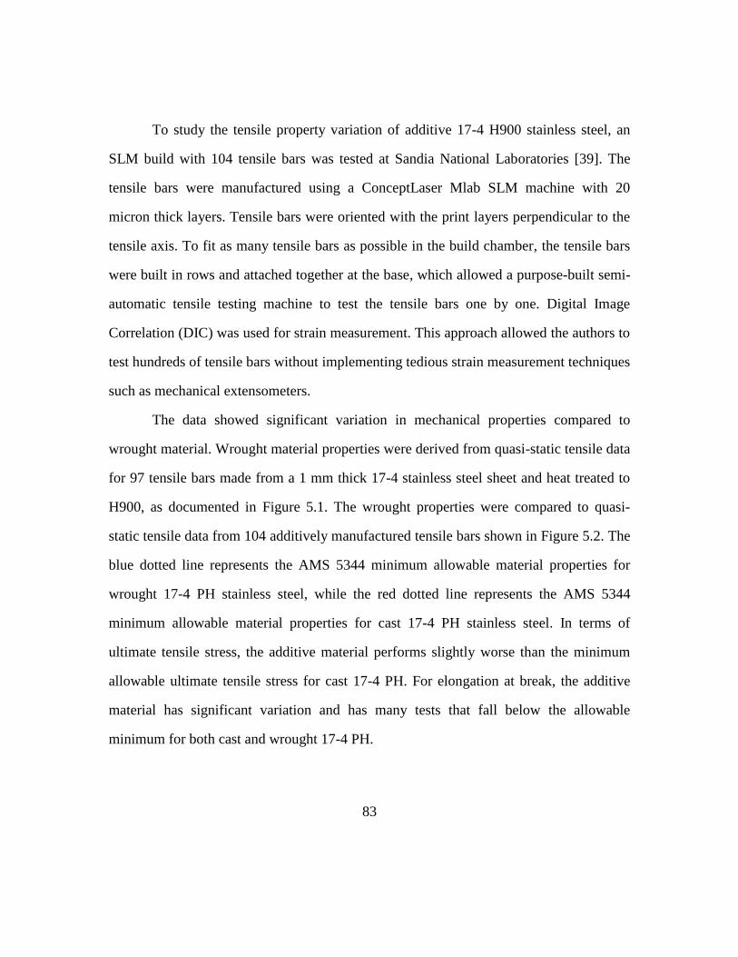
83
To study the tensile property variation of additive 17-4 H900 stainless steel, an
SLM build with 104 tensile bars was tested at Sandia National Laboratories [39]. The
tensile bars were manufactured using a ConceptLaser Mlab SLM machine with 20
micron thick layers. Tensile bars were oriented with the print layers perpendicular to the
tensile axis. To fit as many tensile bars as possible in the build chamber, the tensile bars
were built in rows and attached together at the base, which allowed a purpose-built semi-
automatic tensile testing machine to test the tensile bars one by one. Digital Image
Correlation (DIC) was used for strain measurement. This approach allowed the authors to
test hundreds of tensile bars without implementing tedious strain measurement techniques
such as mechanical extensometers.
The data showed significant variation in mechanical properties compared to
wrought material. Wrought material properties were derived from quasi-static tensile data
for 97 tensile bars made from a 1 mm thick 17-4 stainless steel sheet and heat treated to
H900, as documented in Figure 5.1. The wrought properties were compared to quasi-
static tensile data from 104 additively manufactured tensile bars shown in Figure 5.2. The
blue dotted line represents the AMS 5344 minimum allowable material properties for
wrought 17-4 PH stainless steel, while the red dotted line represents the AMS 5344
minimum allowable material properties for cast 17-4 PH stainless steel. In terms of
ultimate tensile stress, the additive material performs slightly worse than the minimum
allowable ultimate tensile stress for cast 17-4 PH. For elongation at break, the additive
material has significant variation and has many tests that fall below the allowable
minimum for both cast and wrought 17-4 PH.
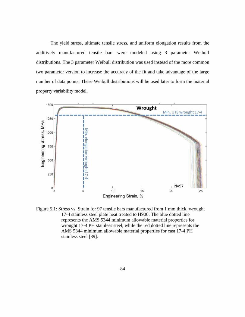
84
The yield stress, ultimate tensile stress, and uniform elongation results from the
additively manufactured tensile bars were modeled using 3 parameter Weibull
distributions. The 3 parameter Weibull distribution was used instead of the more common
two parameter version to increase the accuracy of the fit and take advantage of the large
number of data points. These Weibull distributions will be used later to form the material
property variability model.
Figure 5.1: Stress vs. Strain for 97 tensile bars manufactured from 1 mm thick, wrought
17-4 stainless steel plate heat treated to H900. The blue dotted line
represents the AMS 5344 minimum allowable material properties for
wrought 17-4 PH stainless steel, while the red dotted line represents the
AMS 5344 minimum allowable material properties for cast 17-4 PH
stainless steel [39].
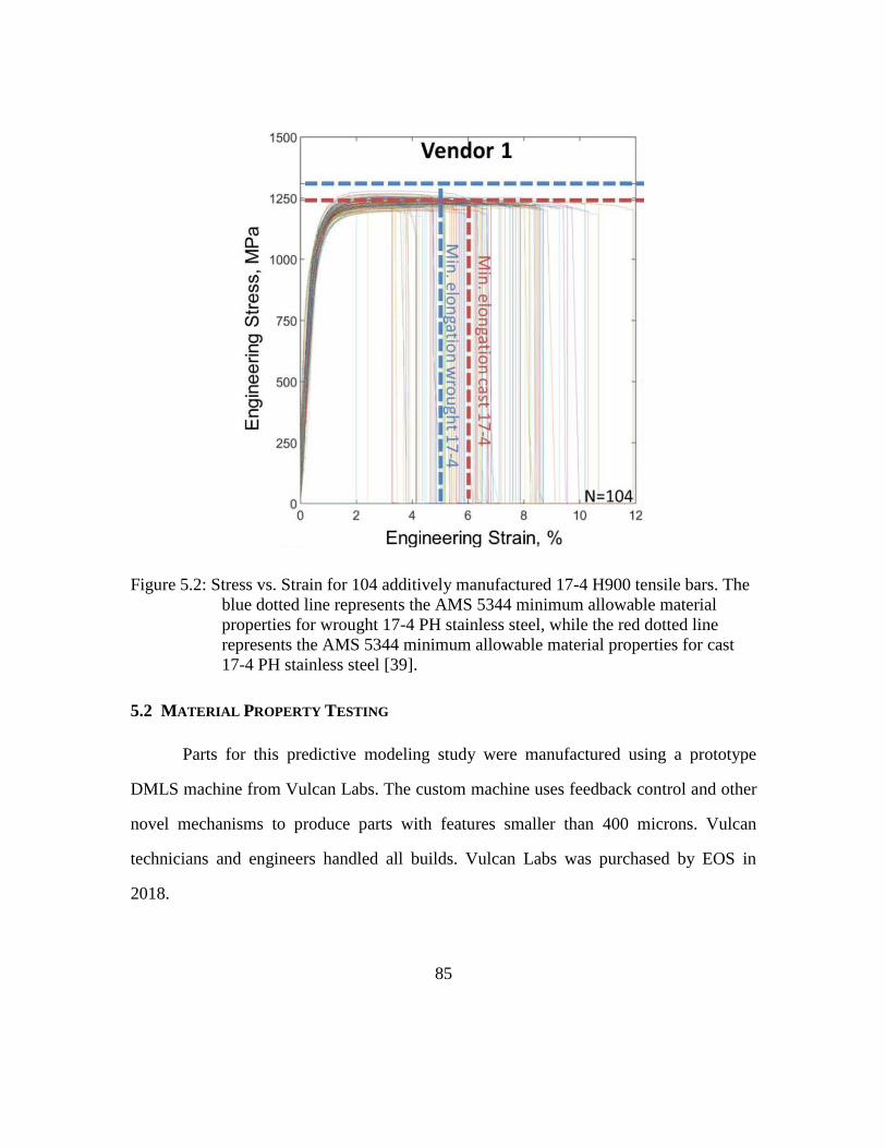
85
Figure 5.2: Stress vs. Strain for 104 additively manufactured 17-4 H900 tensile bars. The
blue dotted line represents the AMS 5344 minimum allowable material
properties for wrought 17-4 PH stainless steel, while the red dotted line
represents the AMS 5344 minimum allowable material properties for cast
17-4 PH stainless steel [39].
5.2 MATERIAL PROPERTY TESTING
Parts for this predictive modeling study were manufactured using a prototype
DMLS machine from Vulcan Labs. The custom machine uses feedback control and other
novel mechanisms to produce parts with features smaller than 400 microns. Vulcan
technicians and engineers handled all builds. Vulcan Labs was purchased by EOS in
2018.

86
Maraging steel (18Ni-300) was used over the common 17-4 stainless steel for this
study to accommodate Vulcan’s testing schedule since Vulcan was fabricating all of the
parts at no cost. Maraging steel has an extremely high yield strain when heat treated, and
a yield strain similar to H1150 17-4 when not heat treated; therefore, it is a suitable
replacement for 17-4 and designs could be quickly adapted to the new material. Heat
treatment was not selected for the parts because of the extreme hardness of heat treated
maraging steel. Tensile specimens could be strong enough to exceed the maximum
strength of tensile testing grips, which could cause the teeth to fail in shear.
Maraging steel tensile bars were produced by machining down two solid blocks of
additively fabricated steel into ASTM E8 sheet metal type tensile bars [40]. The tensile
bars have the ASTM F2971 YZ orientation (Figure 5.3) [28]. Each tensile bar was
extracted from a different build on the same Vulcan machine. Testing was conducted by
Element Materials Technology in Houston, Texas, in accordance with ASTM E8
standards. An extensometer remained on the specimens until shortly before break to
obtain strain data minimally effected by the test equipment.
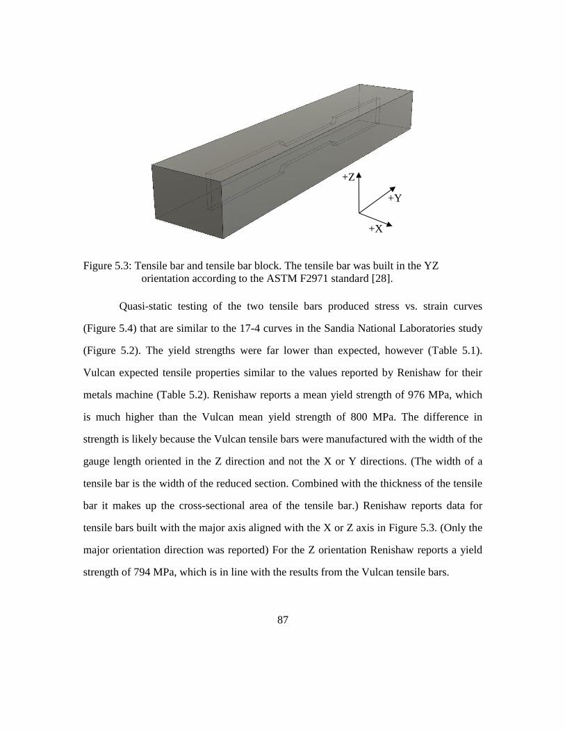
87
Figure 5.3: Tensile bar and tensile bar block. The tensile bar was built in the YZ
orientation according to the ASTM F2971 standard [28].
Quasi-static testing of the two tensile bars produced stress vs. strain curves
(Figure 5.4) that are similar to the 17-4 curves in the Sandia National Laboratories study
(Figure 5.2). The yield strengths were far lower than expected, however (Table 5.1).
Vulcan expected tensile properties similar to the values reported by Renishaw for their
metals machine (Table 5.2). Renishaw reports a mean yield strength of 976 MPa, which
is much higher than the Vulcan mean yield strength of 800 MPa. The difference in
strength is likely because the Vulcan tensile bars were manufactured with the width of the
gauge length oriented in the Z direction and not the X or Y directions. (The width of a
tensile bar is the width of the reduced section. Combined with the thickness of the tensile
bar it makes up the cross-sectional area of the tensile bar.) Renishaw reports data for
tensile bars built with the major axis aligned with the X or Z axis in Figure 5.3. (Only the
major orientation direction was reported) For the Z orientation Renishaw reports a yield
strength of 794 MPa, which is in line with the results from the Vulcan tensile bars.
+Z
+Y
+X
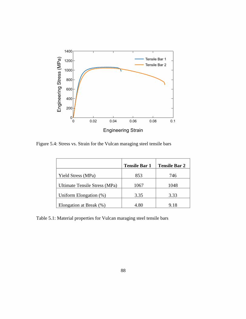
88
Figure 5.4: Stress vs. Strain for the Vulcan maraging steel tensile bars
Tensile Bar 1 Tensile Bar 2
Yield Stress (MPa) 853 746
Ultimate Tensile Stress (MPa) 1067 1048
Uniform Elongation (%) 3.35 3.33
Elongation at Break (%) 4.80 9.18
Table 5.1: Material properties for Vulcan maraging steel tensile bars
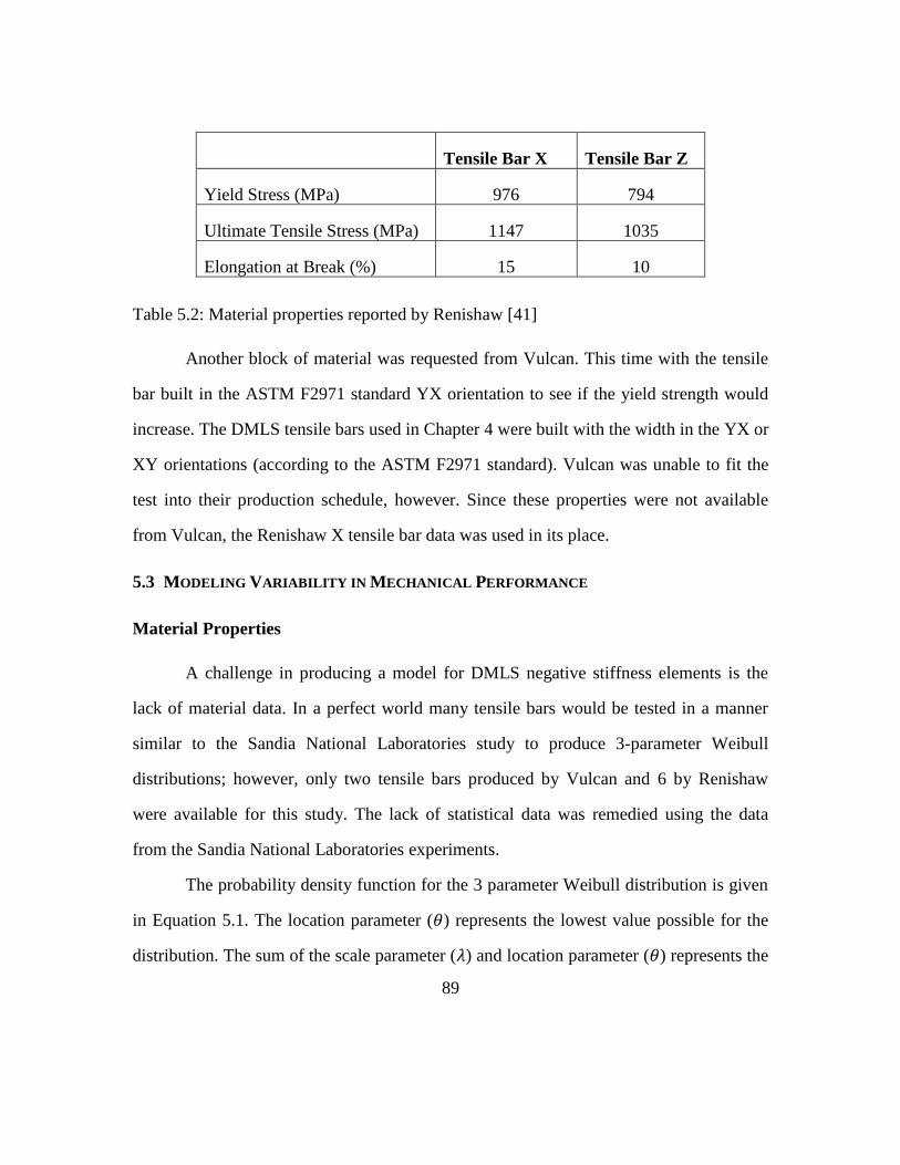
89
Tensile Bar X Tensile Bar Z
Yield Stress (MPa) 976 794
Ultimate Tensile Stress (MPa) 1147 1035
Elongation at Break (%) 15 10
Table 5.2: Material properties reported by Renishaw [41]
Another block of material was requested from Vulcan. This time with the tensile
bar built in the ASTM F2971 standard YX orientation to see if the yield strength would
increase. The DMLS tensile bars used in Chapter 4 were built with the width in the YX or
XY orientations (according to the ASTM F2971 standard). Vulcan was unable to fit the
test into their production schedule, however. Since these properties were not available
from Vulcan, the Renishaw X tensile bar data was used in its place.
5.3 MODELING VARIABILITY IN MECHANICAL PERFORMANCE
Material Properties
A challenge in producing a model for DMLS negative stiffness elements is the
lack of material data. In a perfect world many tensile bars would be tested in a manner
similar to the Sandia National Laboratories study to produce 3-parameter Weibull
distributions; however, only two tensile bars produced by Vulcan and 6 by Renishaw
were available for this study. The lack of statistical data was remedied using the data
from the Sandia National Laboratories experiments.
The probability density function for the 3 parameter Weibull distribution is given
in Equation 5.1. The location parameter (𝜃) represents the lowest value possible for the
distribution. The sum of the scale parameter (𝜆) and location parameter (𝜃) represents the
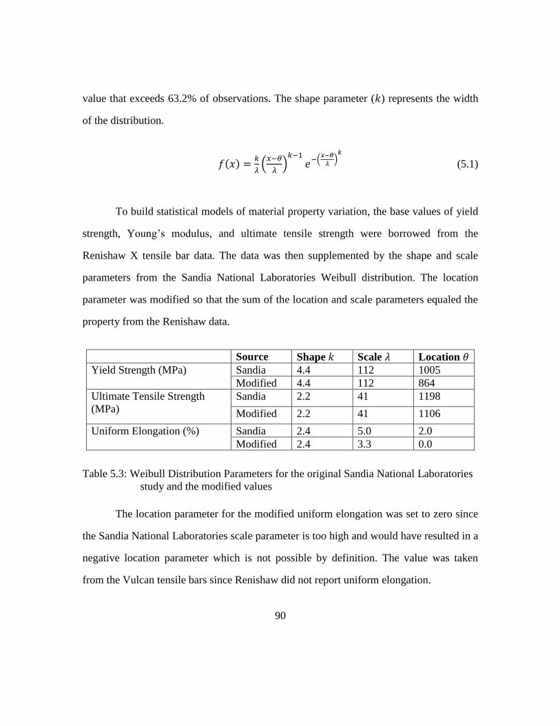
90
value that exceeds 63.2% of observations. The shape parameter (𝑘) represents the width
of the distribution.
𝑓(𝑥) =𝑘
𝜆(
𝑥−𝜃
𝜆)
𝑘−1
𝑒−(𝑥−𝜃
𝜆)
𝑘
(5.1)
To build statistical models of material property variation, the base values of yield
strength, Young’s modulus, and ultimate tensile strength were borrowed from the
Renishaw X tensile bar data. The data was then supplemented by the shape and scale
parameters from the Sandia National Laboratories Weibull distribution. The location
parameter was modified so that the sum of the location and scale parameters equaled the
property from the Renishaw data.
Source Shape 𝑘 Scale 𝜆 Location 𝜃
Yield Strength (MPa) Sandia 4.4 112 1005
Modified 4.4 112 864
Ultimate Tensile Strength
(MPa)
Sandia 2.2 41 1198
Modified 2.2 41 1106
Uniform Elongation (%) Sandia 2.4 5.0 2.0
Modified 2.4 3.3 0.0
Table 5.3: Weibull Distribution Parameters for the original Sandia National Laboratories
study and the modified values
The location parameter for the modified uniform elongation was set to zero since
the Sandia National Laboratories scale parameter is too high and would have resulted in a
negative location parameter which is not possible by definition. The value was taken
from the Vulcan tensile bars since Renishaw did not report uniform elongation.
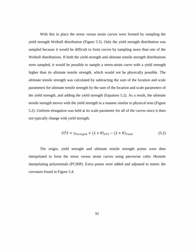
91
With this in place the stress versus strain curves were formed by sampling the
yield strength Weibull distribution (Figure 5.5). Only the yield strength distribution was
sampled because it would be difficult to form curves by sampling more than one of the
Weibull distributions. If both the yield strength and ultimate tensile strength distributions
were sampled, it would be possible to sample a stress-strain curve with a yield strength
higher than its ultimate tensile strength, which would not be physically possible. The
ultimate tensile strength was calculated by subtracting the sum of the location and scale
parameters for ultimate tensile strength by the sum of the location and scale parameters of
the yield strength, and adding the yield strength (Equation 5.2). As a result, the ultimate
tensile strength moves with the yield strength in a manner similar to physical tests (Figure
5.2). Uniform elongation was held at its scale parameter for all of the curves since it does
not typically change with yield strength.
𝑈𝑇𝑆 = 𝑦𝑠𝑡𝑟𝑒𝑛𝑔𝑡ℎ + (𝜆 + 𝜃)𝑈𝑇𝑆 − (𝜆 + 𝜃)𝑌𝑖𝑒𝑙𝑑 (5.2)
The origin, yield strength and ultimate tensile strength points were then
interpolated to form the stress versus strain curves using piecewise cubic Hermite
interpolating polynomials (PCHIP). Extra points were added and adjusted to mimic the
curvature found in Figure 5.4.
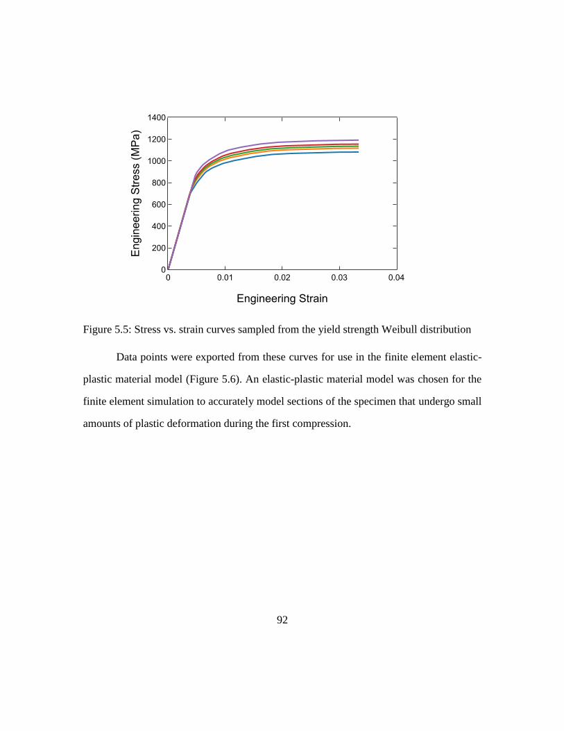
92
Figure 5.5: Stress vs. strain curves sampled from the yield strength Weibull distribution
Data points were exported from these curves for use in the finite element elastic-
plastic material model (Figure 5.6). An elastic-plastic material model was chosen for the
finite element simulation to accurately model sections of the specimen that undergo small
amounts of plastic deformation during the first compression.
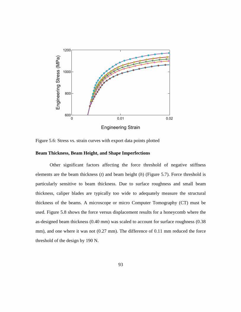
93
Figure 5.6: Stress vs. strain curves with export data points plotted
Beam Thickness, Beam Height, and Shape Imperfections
Other significant factors affecting the force threshold of negative stiffness
elements are the beam thickness (t) and beam height (h) (Figure 5.7). Force threshold is
particularly sensitive to beam thickness. Due to surface roughness and small beam
thickness, caliper blades are typically too wide to adequately measure the structural
thickness of the beams. A microscope or micro Computer Tomography (CT) must be
used. Figure 5.8 shows the force versus displacement results for a honeycomb where the
as-designed beam thickness (0.40 mm) was scaled to account for surface roughness (0.38
mm), and one where it was not (0.27 mm). The difference of 0.11 mm reduced the force
threshold of the design by 190 N.
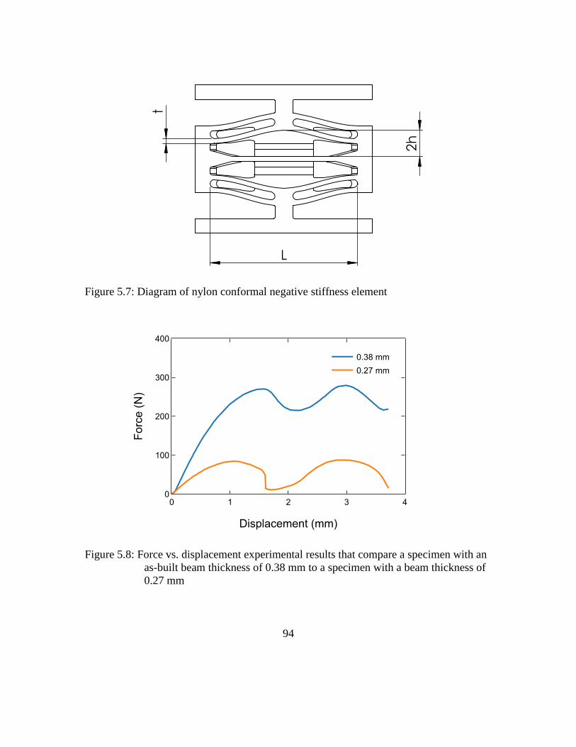
94
Figure 5.7: Diagram of nylon conformal negative stiffness element
Figure 5.8: Force vs. displacement experimental results that compare a specimen with an
as-built beam thickness of 0.38 mm to a specimen with a beam thickness of
0.27 mm
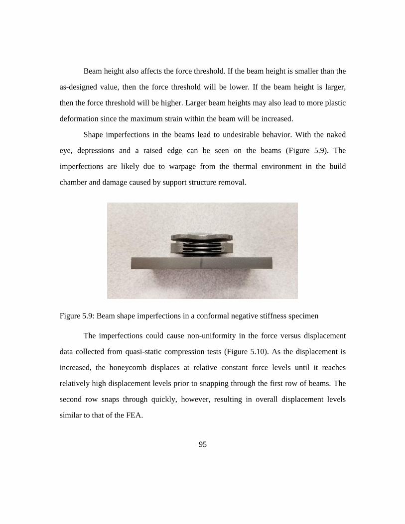
95
Beam height also affects the force threshold. If the beam height is smaller than the
as-designed value, then the force threshold will be lower. If the beam height is larger,
then the force threshold will be higher. Larger beam heights may also lead to more plastic
deformation since the maximum strain within the beam will be increased.
Shape imperfections in the beams lead to undesirable behavior. With the naked
eye, depressions and a raised edge can be seen on the beams (Figure 5.9). The
imperfections are likely due to warpage from the thermal environment in the build
chamber and damage caused by support structure removal.
Figure 5.9: Beam shape imperfections in a conformal negative stiffness specimen
The imperfections could cause non-uniformity in the force versus displacement
data collected from quasi-static compression tests (Figure 5.10). As the displacement is
increased, the honeycomb displaces at relative constant force levels until it reaches
relatively high displacement levels prior to snapping through the first row of beams. The
second row snaps through quickly, however, resulting in overall displacement levels
similar to that of the FEA.
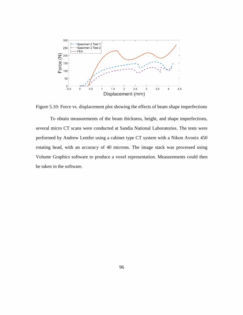
96
Figure 5.10: Force vs. displacement plot showing the effects of beam shape imperfections
To obtain measurements of the beam thickness, height, and shape imperfections,
several micro CT scans were conducted at Sandia National Laboratories. The tests were
performed by Andrew Lentfer using a cabinet type CT system with a Nikon Avonix 450
rotating head, with an accuracy of 40 microns. The image stack was processed using
Volume Graphics software to produce a voxel representation. Measurements could then
be taken in the software.
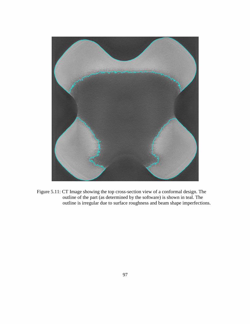
97
Figure 5.11: CT Image showing the top cross-section view of a conformal design. The
outline of the part (as determined by the software) is shown in teal. The
outline is irregular due to surface roughness and beam shape imperfections.
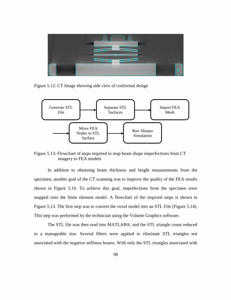
98
Figure 5.12: CT Image showing side view of conformal design
Figure 5.13: Flowchart of steps required to map beam shape imperfections from CT
imagery to FEA models
In addition to obtaining beam thickness and height measurements from the
specimen, another goal of the CT scanning was to improve the quality of the FEA results
shown in Figure 5.10. To achieve this goal, imperfections from the specimen were
mapped onto the finite element model. A flowchart of the required steps is shown in
Figure 5.13. The first step was to convert the voxel model into an STL File (Figure 5.14).
This step was performed by the technician using the Volume Graphics software.
The STL file was then read into MATLAB®, and the STL triangle count reduced
to a manageable size. Several filters were applied to eliminate STL triangles not
associated with the negative stiffness beams. With only the STL triangles associated with
Generate STL
File
Separate STL
Surfaces
Import FEA
Mesh
Move FEA
Nodes to STL
Surface
Run Abaqus
Simulation
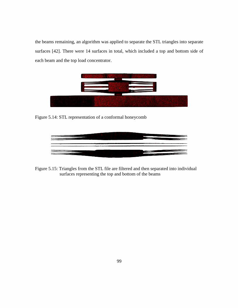
99
the beams remaining, an algorithm was applied to separate the STL triangles into separate
surfaces [42]. There were 14 surfaces in total, which included a top and bottom side of
each beam and the top load concentrator.
Figure 5.14: STL representation of a conformal honeycomb
Figure 5.15: Triangles from the STL file are filtered and then separated into individual
surfaces representing the top and bottom of the beams
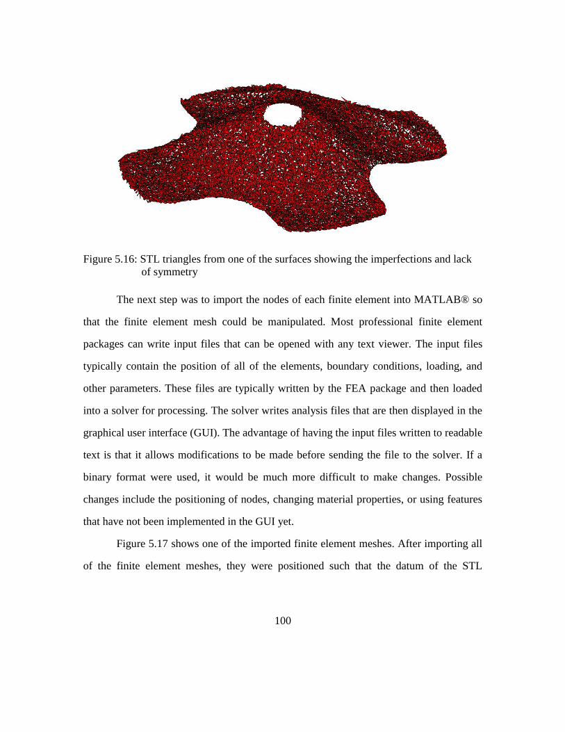
100
Figure 5.16: STL triangles from one of the surfaces showing the imperfections and lack
of symmetry
The next step was to import the nodes of each finite element into MATLAB® so
that the finite element mesh could be manipulated. Most professional finite element
packages can write input files that can be opened with any text viewer. The input files
typically contain the position of all of the elements, boundary conditions, loading, and
other parameters. These files are typically written by the FEA package and then loaded
into a solver for processing. The solver writes analysis files that are then displayed in the
graphical user interface (GUI). The advantage of having the input files written to readable
text is that it allows modifications to be made before sending the file to the solver. If a
binary format were used, it would be much more difficult to make changes. Possible
changes include the positioning of nodes, changing material properties, or using features
that have not been implemented in the GUI yet.
Figure 5.17 shows one of the imported finite element meshes. After importing all
of the finite element meshes, they were positioned such that the datum of the STL
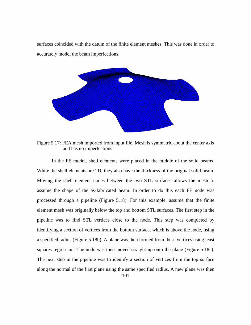
101
surfaces coincided with the datum of the finite element meshes. This was done in order to
accurately model the beam imperfections.
Figure 5.17: FEA mesh imported from input file. Mesh is symmetric about the center axis
and has no imperfections
In the FE model, shell elements were placed in the middle of the solid beams.
While the shell elements are 2D, they also have the thickness of the original solid beam.
Moving the shell element nodes between the two STL surfaces allows the mesh to
assume the shape of the as-fabricated beam. In order to do this each FE node was
processed through a pipeline (Figure 5.18). For this example, assume that the finite
element mesh was originally below the top and bottom STL surfaces. The first step in the
pipeline was to find STL vertices close to the node. This step was completed by
identifying a section of vertices from the bottom surface, which is above the node, using
a specified radius (Figure 5.18b). A plane was then formed from these vertices using least
squares regression. The node was then moved straight up onto the plane (Figure 5.18c).
The next step in the pipeline was to identify a section of vertices from the top surface
along the normal of the first plane using the same specified radius. A new plane was then
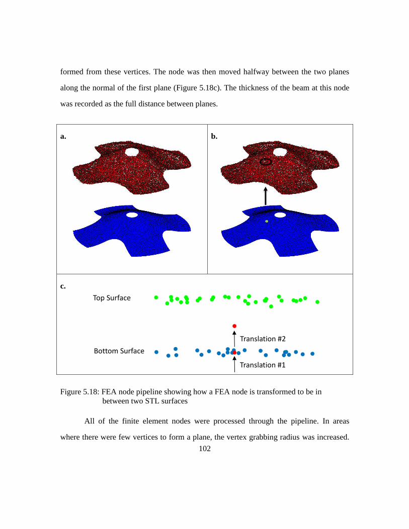
102
formed from these vertices. The node was then moved halfway between the two planes
along the normal of the first plane (Figure 5.18c). The thickness of the beam at this node
was recorded as the full distance between planes.
a.
b.
c.
Figure 5.18: FEA node pipeline showing how a FEA node is transformed to be in
between two STL surfaces
All of the finite element nodes were processed through the pipeline. In areas
where there were few vertices to form a plane, the vertex grabbing radius was increased.
Bottom Surface
Top Surface
Translation #2
Translation #1
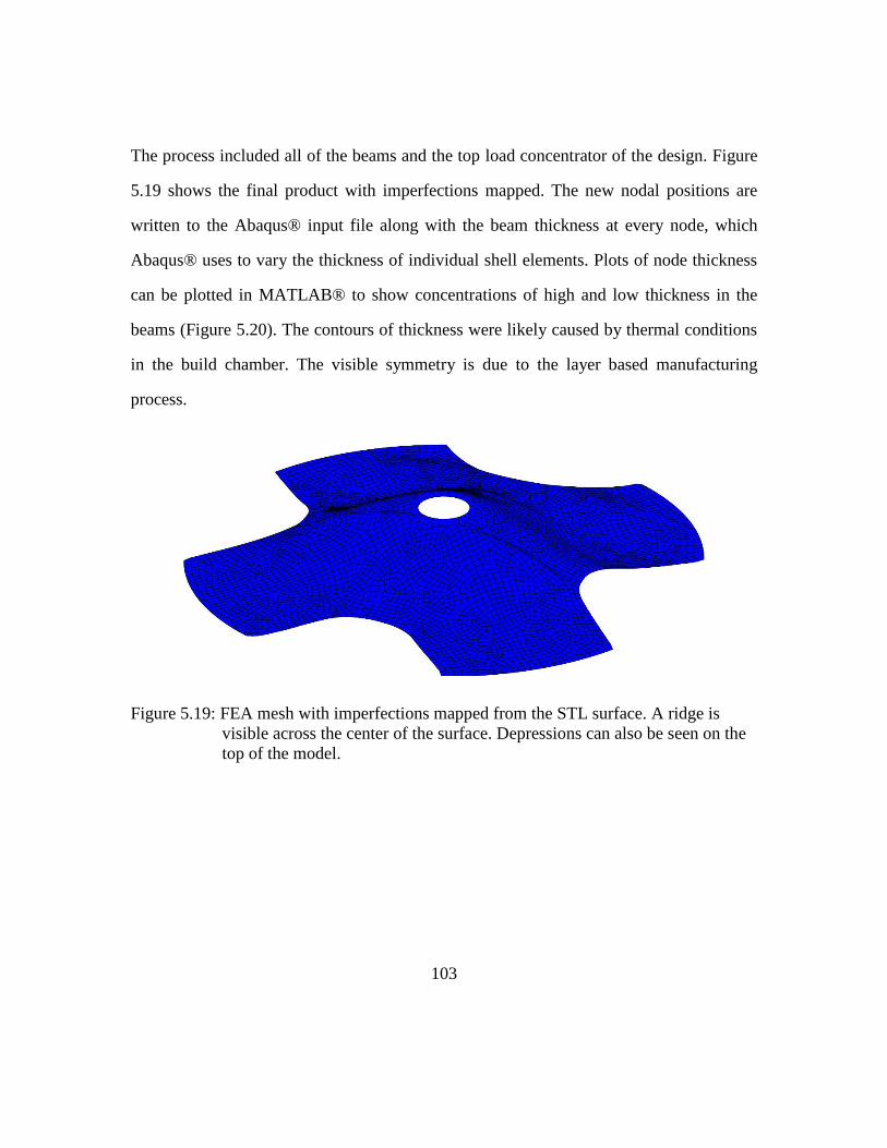
103
The process included all of the beams and the top load concentrator of the design. Figure
5.19 shows the final product with imperfections mapped. The new nodal positions are
written to the Abaqus® input file along with the beam thickness at every node, which
Abaqus® uses to vary the thickness of individual shell elements. Plots of node thickness
can be plotted in MATLAB® to show concentrations of high and low thickness in the
beams (Figure 5.20). The contours of thickness were likely caused by thermal conditions
in the build chamber. The visible symmetry is due to the layer based manufacturing
process.
Figure 5.19: FEA mesh with imperfections mapped from the STL surface. A ridge is
visible across the center of the surface. Depressions can also be seen on the
top of the model.
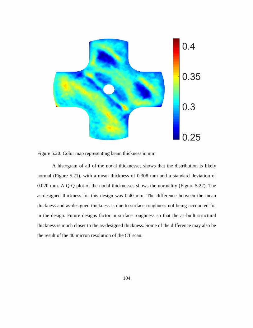
104
Figure 5.20: Color map representing beam thickness in mm
A histogram of all of the nodal thicknesses shows that the distribution is likely
normal (Figure 5.21), with a mean thickness of 0.308 mm and a standard deviation of
0.020 mm. A Q-Q plot of the nodal thicknesses shows the normality (Figure 5.22). The
as-designed thickness for this design was 0.40 mm. The difference between the mean
thickness and as-designed thickness is due to surface roughness not being accounted for
in the design. Future designs factor in surface roughness so that the as-built structural
thickness is much closer to the as-designed thickness. Some of the difference may also be
the result of the 40 micron resolution of the CT scan.
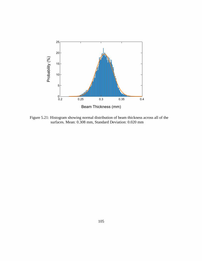
105
Figure 5.21: Histogram showing normal distribution of beam thickness across all of the
surfaces. Mean: 0.308 mm, Standard Deviation: 0.020 mm
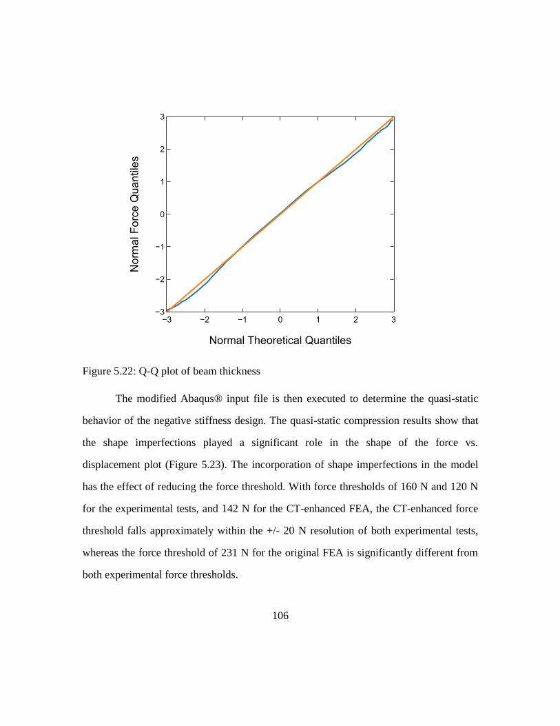
106
Figure 5.22: Q-Q plot of beam thickness
The modified Abaqus® input file is then executed to determine the quasi-static
behavior of the negative stiffness design. The quasi-static compression results show that
the shape imperfections played a significant role in the shape of the force vs.
displacement plot (Figure 5.23). The incorporation of shape imperfections in the model
has the effect of reducing the force threshold. With force thresholds of 160 N and 120 N
for the experimental tests, and 142 N for the CT-enhanced FEA, the CT-enhanced force
threshold falls approximately within the +/- 20 N resolution of both experimental tests,
whereas the force threshold of 231 N for the original FEA is significantly different from
both experimental force thresholds.
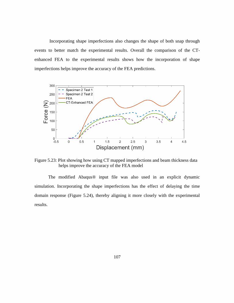
107
Incorporating shape imperfections also changes the shape of both snap through
events to better match the experimental results. Overall the comparison of the CT-
enhanced FEA to the experimental results shows how the incorporation of shape
imperfections helps improve the accuracy of the FEA predictions.
Figure 5.23: Plot showing how using CT mapped imperfections and beam thickness data
helps improve the accuracy of the FEA model
The modified Abaqus® input file was also used in an explicit dynamic
simulation. Incorporating the shape imperfections has the effect of delaying the time
domain response (Figure 5.24), thereby aligning it more closely with the experimental
results.
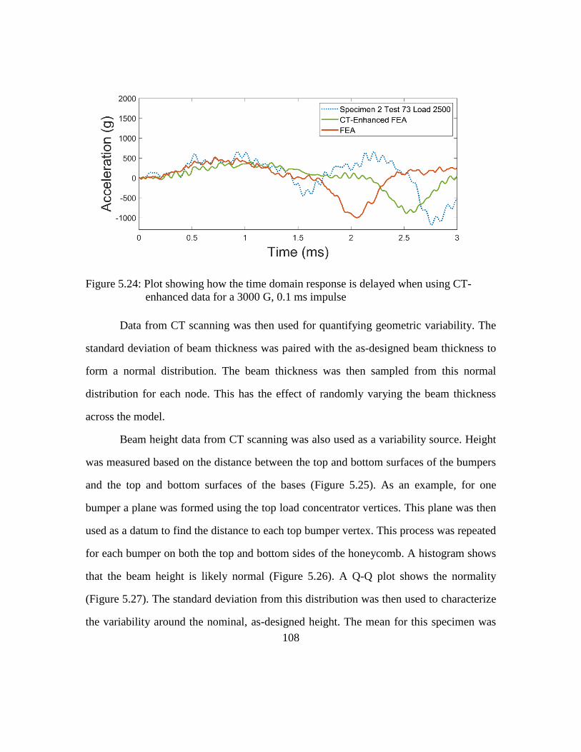
108
Figure 5.24: Plot showing how the time domain response is delayed when using CT-
enhanced data for a 3000 G, 0.1 ms impulse
Data from CT scanning was then used for quantifying geometric variability. The
standard deviation of beam thickness was paired with the as-designed beam thickness to
form a normal distribution. The beam thickness was then sampled from this normal
distribution for each node. This has the effect of randomly varying the beam thickness
across the model.
Beam height data from CT scanning was also used as a variability source. Height
was measured based on the distance between the top and bottom surfaces of the bumpers
and the top and bottom surfaces of the bases (Figure 5.25). As an example, for one
bumper a plane was formed using the top load concentrator vertices. This plane was then
used as a datum to find the distance to each top bumper vertex. This process was repeated
for each bumper on both the top and bottom sides of the honeycomb. A histogram shows
that the beam height is likely normal (Figure 5.26). A Q-Q plot shows the normality
(Figure 5.27). The standard deviation from this distribution was then used to characterize
the variability around the nominal, as-designed height. The mean for this specimen was
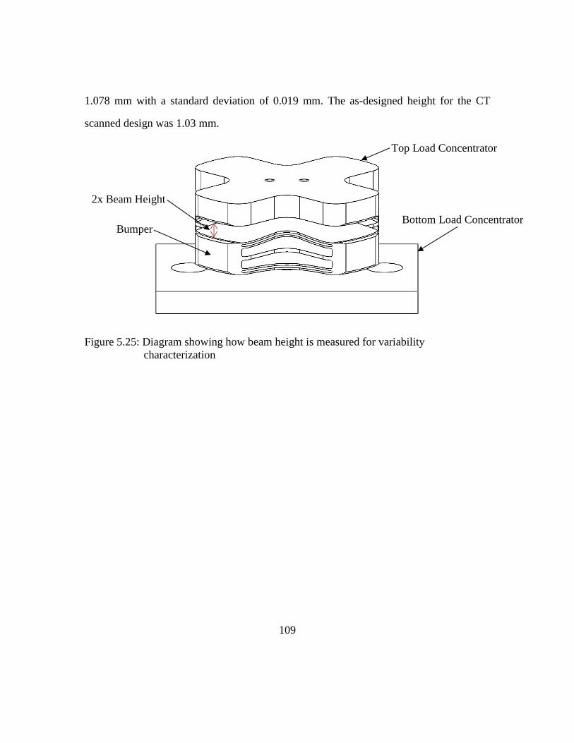
109
1.078 mm with a standard deviation of 0.019 mm. The as-designed height for the CT
scanned design was 1.03 mm.
Figure 5.25: Diagram showing how beam height is measured for variability
characterization
2x Beam Height
Bumper
Top Load Concentrator
Bottom Load Concentrator
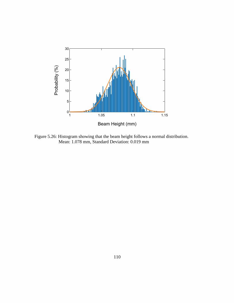
110
Figure 5.26: Histogram showing that the beam height follows a normal distribution.
Mean: 1.078 mm, Standard Deviation: 0.019 mm
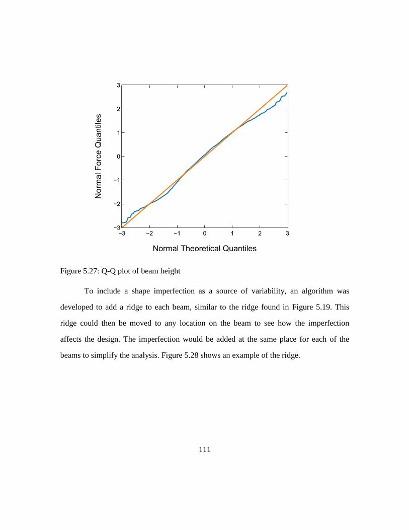
111
Figure 5.27: Q-Q plot of beam height
To include a shape imperfection as a source of variability, an algorithm was
developed to add a ridge to each beam, similar to the ridge found in Figure 5.19. This
ridge could then be moved to any location on the beam to see how the imperfection
affects the design. The imperfection would be added at the same place for each of the
beams to simplify the analysis. Figure 5.28 shows an example of the ridge.
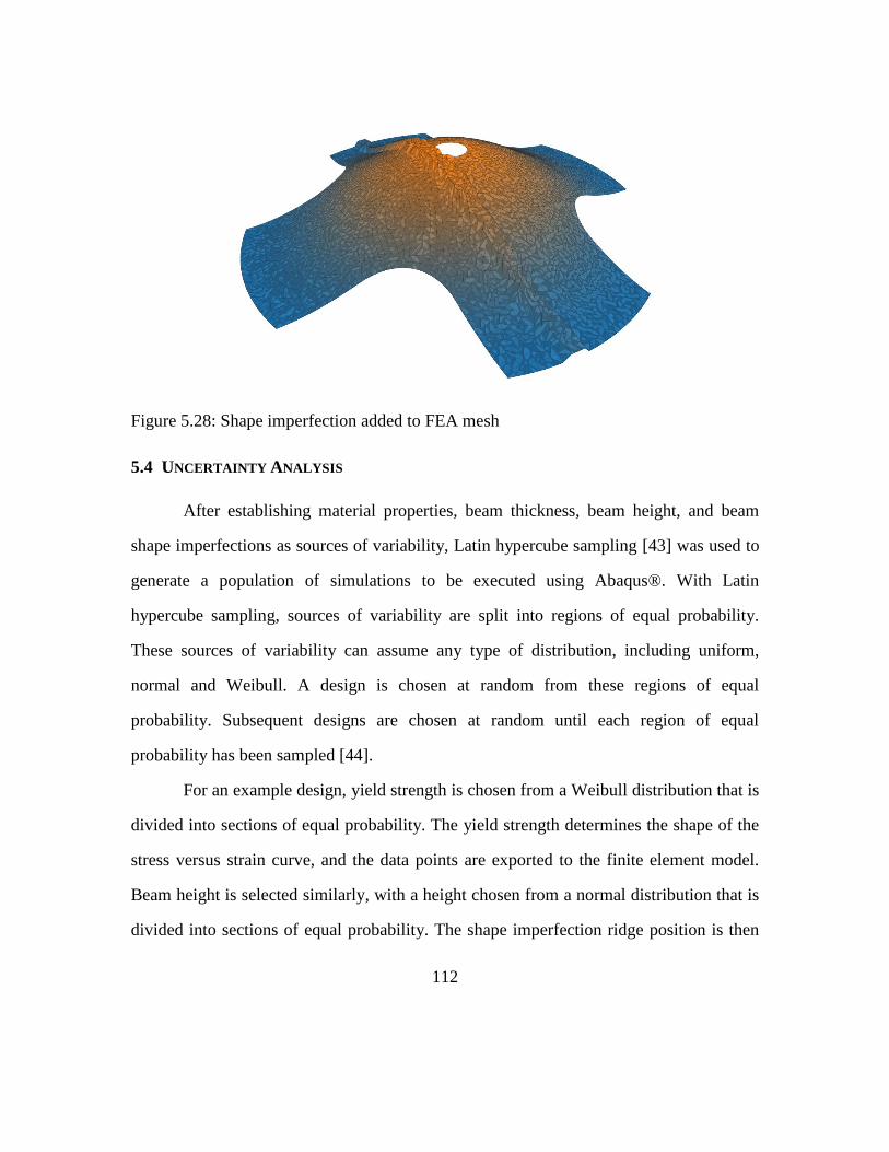
112
Figure 5.28: Shape imperfection added to FEA mesh
5.4 UNCERTAINTY ANALYSIS
After establishing material properties, beam thickness, beam height, and beam
shape imperfections as sources of variability, Latin hypercube sampling [43] was used to
generate a population of simulations to be executed using Abaqus®. With Latin
hypercube sampling, sources of variability are split into regions of equal probability.
These sources of variability can assume any type of distribution, including uniform,
normal and Weibull. A design is chosen at random from these regions of equal
probability. Subsequent designs are chosen at random until each region of equal
probability has been sampled [44].
For an example design, yield strength is chosen from a Weibull distribution that is
divided into sections of equal probability. The yield strength determines the shape of the
stress versus strain curve, and the data points are exported to the finite element model.
Beam height is selected similarly, with a height chosen from a normal distribution that is
divided into sections of equal probability. The shape imperfection ridge position is then
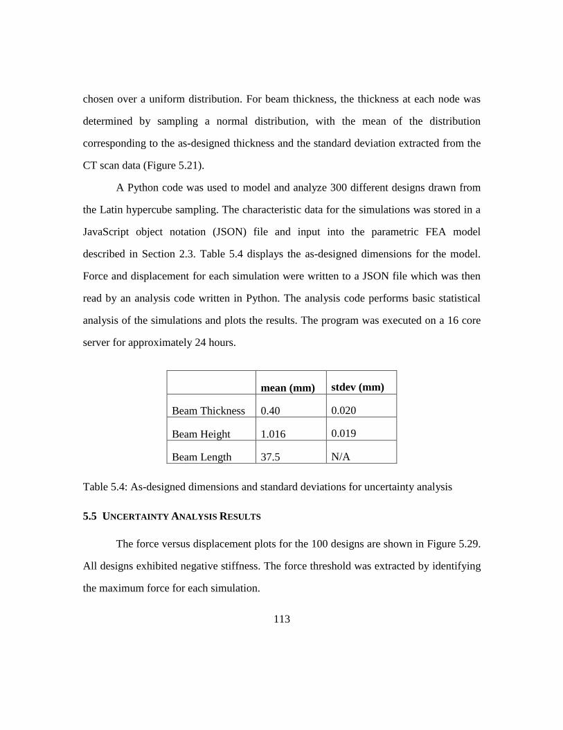
113
chosen over a uniform distribution. For beam thickness, the thickness at each node was
determined by sampling a normal distribution, with the mean of the distribution
corresponding to the as-designed thickness and the standard deviation extracted from the
CT scan data (Figure 5.21).
A Python code was used to model and analyze 300 different designs drawn from
the Latin hypercube sampling. The characteristic data for the simulations was stored in a
JavaScript object notation (JSON) file and input into the parametric FEA model
described in Section 2.3. Table 5.4 displays the as-designed dimensions for the model.
Force and displacement for each simulation were written to a JSON file which was then
read by an analysis code written in Python. The analysis code performs basic statistical
analysis of the simulations and plots the results. The program was executed on a 16 core
server for approximately 24 hours.
mean (mm) stdev (mm)
Beam Thickness 0.40 0.020
Beam Height 1.016 0.019
Beam Length 37.5 N/A
Table 5.4: As-designed dimensions and standard deviations for uncertainty analysis
5.5 UNCERTAINTY ANALYSIS RESULTS
The force versus displacement plots for the 100 designs are shown in Figure 5.29.
All designs exhibited negative stiffness. The force threshold was extracted by identifying
the maximum force for each simulation.
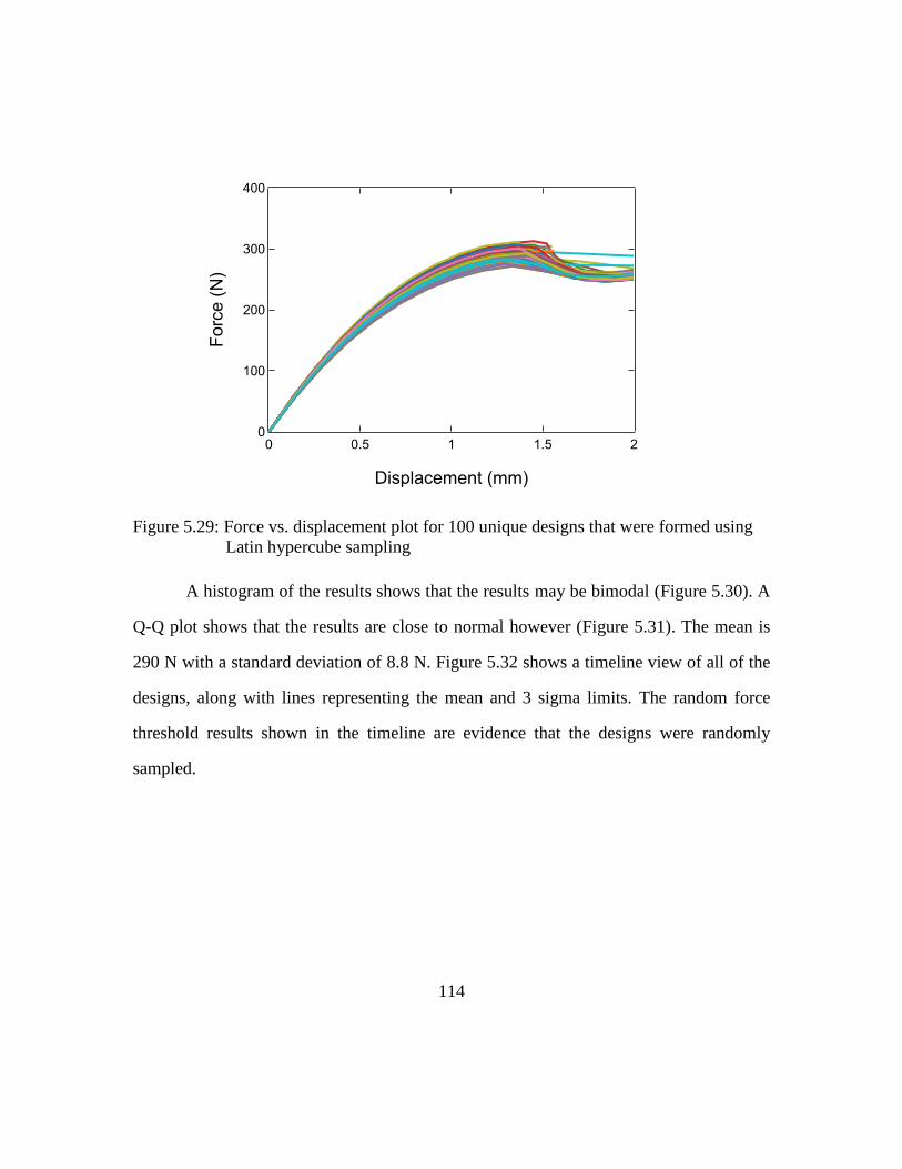
114
Figure 5.29: Force vs. displacement plot for 100 unique designs that were formed using
Latin hypercube sampling
A histogram of the results shows that the results may be bimodal (Figure 5.30). A
Q-Q plot shows that the results are close to normal however (Figure 5.31). The mean is
290 N with a standard deviation of 8.8 N. Figure 5.32 shows a timeline view of all of the
designs, along with lines representing the mean and 3 sigma limits. The random force
threshold results shown in the timeline are evidence that the designs were randomly
sampled.
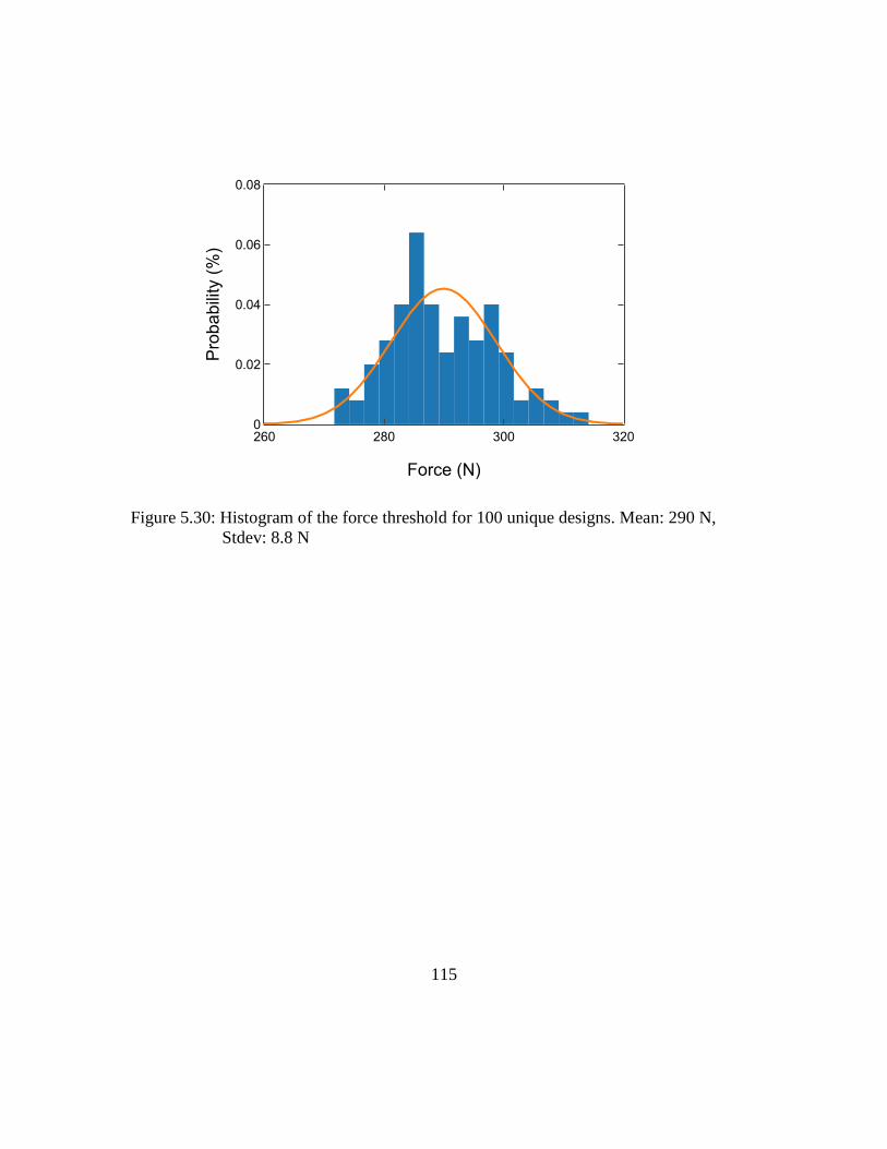
115
Figure 5.30: Histogram of the force threshold for 100 unique designs. Mean: 290 N,
Stdev: 8.8 N
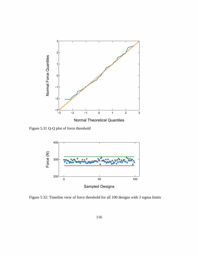
116
Figure 5.31 Q-Q plot of force threshold
Figure 5.32: Timeline view of force threshold for all 100 designs with 3 sigma limits
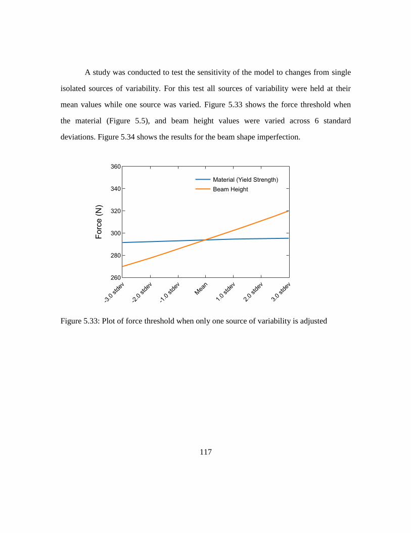
117
A study was conducted to test the sensitivity of the model to changes from single
isolated sources of variability. For this test all sources of variability were held at their
mean values while one source was varied. Figure 5.33 shows the force threshold when
the material (Figure 5.5), and beam height values were varied across 6 standard
deviations. Figure 5.34 shows the results for the beam shape imperfection.
Figure 5.33: Plot of force threshold when only one source of variability is adjusted
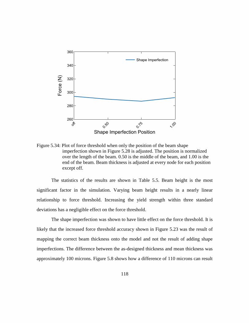
118
Figure 5.34: Plot of force threshold when only the position of the beam shape
imperfection shown in Figure 5.28 is adjusted. The position is normalized
over the length of the beam. 0.50 is the middle of the beam, and 1.00 is the
end of the beam. Beam thickness is adjusted at every node for each position
except off.
The statistics of the results are shown in Table 5.5. Beam height is the most
significant factor in the simulation. Varying beam height results in a nearly linear
relationship to force threshold. Increasing the yield strength within three standard
deviations has a negligible effect on the force threshold.
The shape imperfection was shown to have little effect on the force threshold. It is
likely that the increased force threshold accuracy shown in Figure 5.23 was the result of
mapping the correct beam thickness onto the model and not the result of adding shape
imperfections. The difference between the as-designed thickness and mean thickness was
approximately 100 microns. Figure 5.8 shows how a difference of 110 microns can result
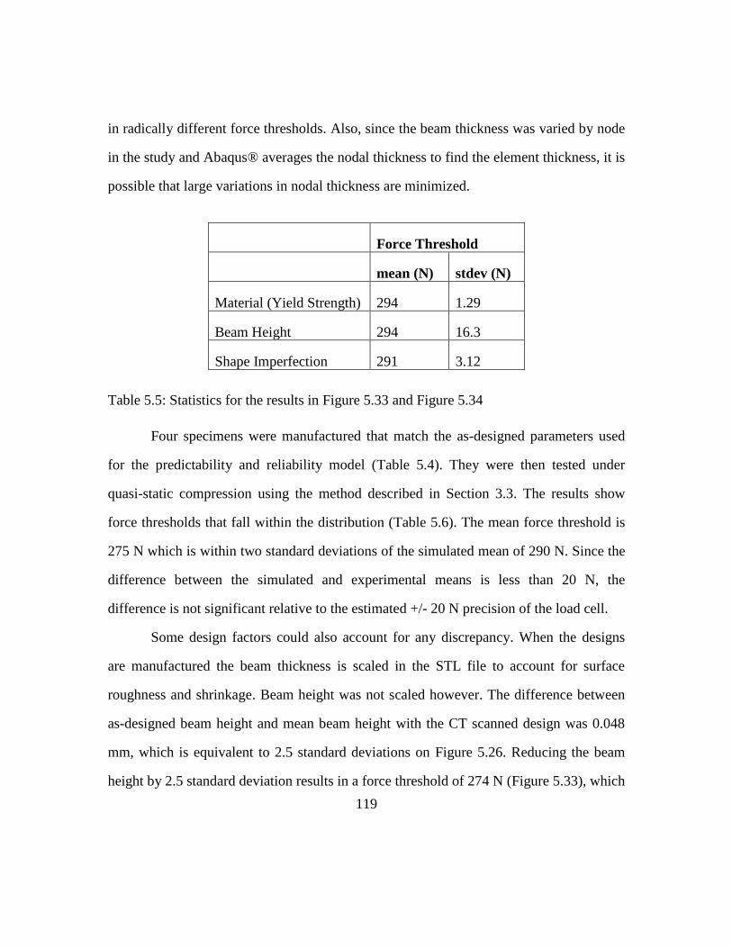
119
in radically different force thresholds. Also, since the beam thickness was varied by node
in the study and Abaqus® averages the nodal thickness to find the element thickness, it is
possible that large variations in nodal thickness are minimized.
Force Threshold
mean (N) stdev (N)
Material (Yield Strength) 294 1.29
Beam Height 294 16.3
Shape Imperfection 291 3.12
Table 5.5: Statistics for the results in Figure 5.33 and Figure 5.34
Four specimens were manufactured that match the as-designed parameters used
for the predictability and reliability model (Table 5.4). They were then tested under
quasi-static compression using the method described in Section 3.3. The results show
force thresholds that fall within the distribution (Table 5.6). The mean force threshold is
275 N which is within two standard deviations of the simulated mean of 290 N. Since the
difference between the simulated and experimental means is less than 20 N, the
difference is not significant relative to the estimated +/- 20 N precision of the load cell.
Some design factors could also account for any discrepancy. When the designs
are manufactured the beam thickness is scaled in the STL file to account for surface
roughness and shrinkage. Beam height was not scaled however. The difference between
as-designed beam height and mean beam height with the CT scanned design was 0.048
mm, which is equivalent to 2.5 standard deviations on Figure 5.26. Reducing the beam
height by 2.5 standard deviation results in a force threshold of 274 N (Figure 5.33), which
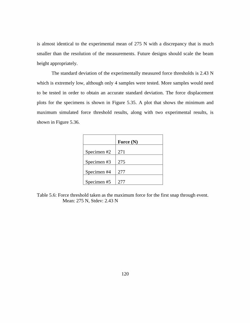
120
is almost identical to the experimental mean of 275 N with a discrepancy that is much
smaller than the resolution of the measurements. Future designs should scale the beam
height appropriately.
The standard deviation of the experimentally measured force thresholds is 2.43 N
which is extremely low, although only 4 samples were tested. More samples would need
to be tested in order to obtain an accurate standard deviation. The force displacement
plots for the specimens is shown in Figure 5.35. A plot that shows the minimum and
maximum simulated force threshold results, along with two experimental results, is
shown in Figure 5.36.
Force (N)
Specimen #2 271
Specimen #3 275
Specimen #4 277
Specimen #5 277
Table 5.6: Force threshold taken as the maximum force for the first snap through event.
Mean: 275 N, Stdev: 2.43 N
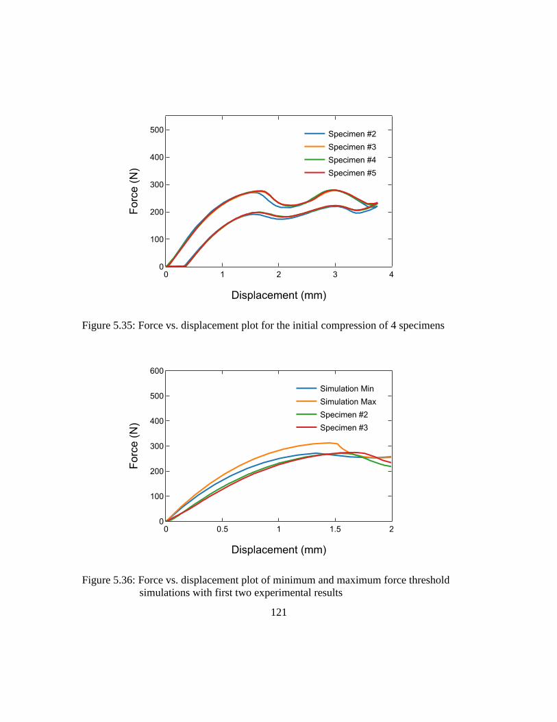
121
Figure 5.35: Force vs. displacement plot for the initial compression of 4 specimens
Figure 5.36: Force vs. displacement plot of minimum and maximum force threshold
simulations with first two experimental results
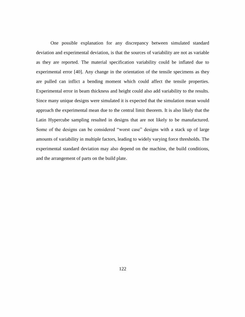
122
One possible explanation for any discrepancy between simulated standard
deviation and experimental deviation, is that the sources of variability are not as variable
as they are reported. The material specification variability could be inflated due to
experimental error [40]. Any change in the orientation of the tensile specimens as they
are pulled can inflict a bending moment which could affect the tensile properties.
Experimental error in beam thickness and height could also add variability to the results.
Since many unique designs were simulated it is expected that the simulation mean would
approach the experimental mean due to the central limit theorem. It is also likely that the
Latin Hypercube sampling resulted in designs that are not likely to be manufactured.
Some of the designs can be considered “worst case” designs with a stack up of large
amounts of variability in multiple factors, leading to widely varying force thresholds. The
experimental standard deviation may also depend on the machine, the build conditions,
and the arrangement of parts on the build plate.
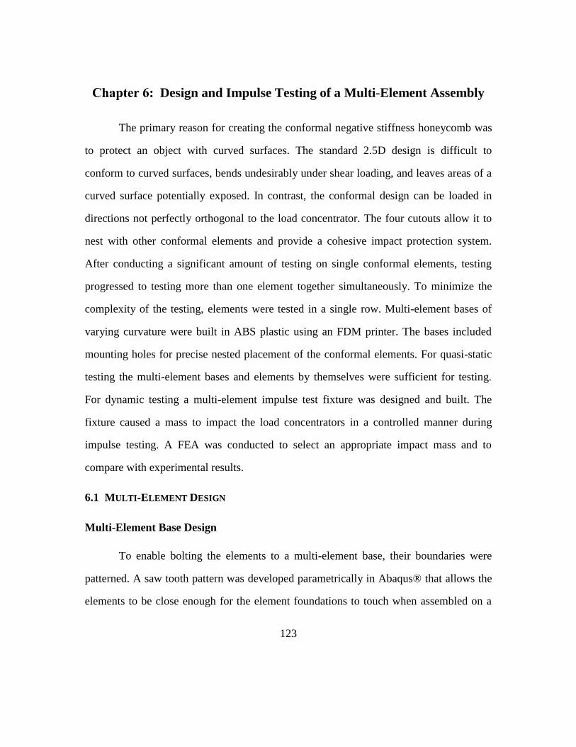
123
Design and Impulse Testing of a Multi-Element Assembly
The primary reason for creating the conformal negative stiffness honeycomb was
to protect an object with curved surfaces. The standard 2.5D design is difficult to
conform to curved surfaces, bends undesirably under shear loading, and leaves areas of a
curved surface potentially exposed. In contrast, the conformal design can be loaded in
directions not perfectly orthogonal to the load concentrator. The four cutouts allow it to
nest with other conformal elements and provide a cohesive impact protection system.
After conducting a significant amount of testing on single conformal elements, testing
progressed to testing more than one element together simultaneously. To minimize the
complexity of the testing, elements were tested in a single row. Multi-element bases of
varying curvature were built in ABS plastic using an FDM printer. The bases included
mounting holes for precise nested placement of the conformal elements. For quasi-static
testing the multi-element bases and elements by themselves were sufficient for testing.
For dynamic testing a multi-element impulse test fixture was designed and built. The
fixture caused a mass to impact the load concentrators in a controlled manner during
impulse testing. A FEA was conducted to select an appropriate impact mass and to
compare with experimental results.
6.1 MULTI-ELEMENT DESIGN
Multi-Element Base Design
To enable bolting the elements to a multi-element base, their boundaries were
patterned. A saw tooth pattern was developed parametrically in Abaqus® that allows the
elements to be close enough for the element foundations to touch when assembled on a
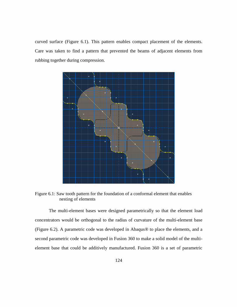
124
curved surface (Figure 6.1). This pattern enables compact placement of the elements.
Care was taken to find a pattern that prevented the beams of adjacent elements from
rubbing together during compression.
Figure 6.1: Saw tooth pattern for the foundation of a conformal element that enables
nesting of elements
The multi-element bases were designed parametrically so that the element load
concentrators would be orthogonal to the radius of curvature of the multi-element base
(Figure 6.2). A parametric code was developed in Abaqus® to place the elements, and a
second parametric code was developed in Fusion 360 to make a solid model of the multi-
element base that could be additively manufactured. Fusion 360 is a set of parametric
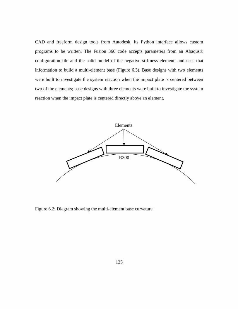
125
CAD and freeform design tools from Autodesk. Its Python interface allows custom
programs to be written. The Fusion 360 code accepts parameters from an Abaqus®
configuration file and the solid model of the negative stiffness element, and uses that
information to build a multi-element base (Figure 6.3). Base designs with two elements
were built to investigate the system reaction when the impact plate is centered between
two of the elements; base designs with three elements were built to investigate the system
reaction when the impact plate is centered directly above an element.
Figure 6.2: Diagram showing the multi-element base curvature
R300
Elements
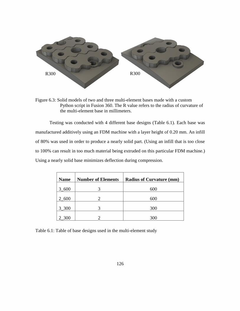
126
Figure 6.3: Solid models of two and three multi-element bases made with a custom
Python script in Fusion 360. The R value refers to the radius of curvature of
the multi-element base in millimeters.
Testing was conducted with 4 different base designs (Table 6.1). Each base was
manufactured additively using an FDM machine with a layer height of 0.20 mm. An infill
of 80% was used in order to produce a nearly solid part. (Using an infill that is too close
to 100% can result in too much material being extruded on this particular FDM machine.)
Using a nearly solid base minimizes deflection during compression.
Name Number of Elements Radius of Curvature (mm)
3_600 3 600
2_600 2 600
3_300 3 300
2_300 2 300
Table 6.1: Table of base designs used in the multi-element study
R300 R300
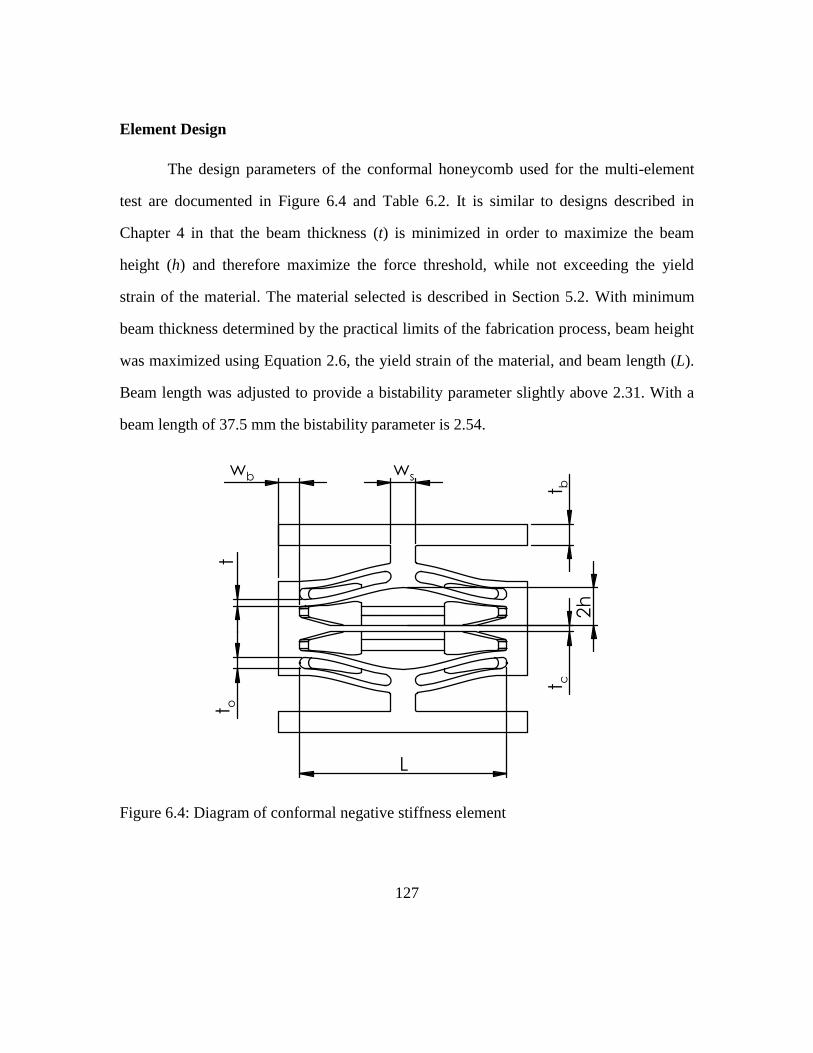
127
Element Design
The design parameters of the conformal honeycomb used for the multi-element
test are documented in Figure 6.4 and Table 6.2. It is similar to designs described in
Chapter 4 in that the beam thickness (t) is minimized in order to maximize the beam
height (h) and therefore maximize the force threshold, while not exceeding the yield
strain of the material. The material selected is described in Section 5.2. With minimum
beam thickness determined by the practical limits of the fabrication process, beam height
was maximized using Equation 2.6, the yield strain of the material, and beam length (L).
Beam length was adjusted to provide a bistability parameter slightly above 2.31. With a
beam length of 37.5 mm the bistability parameter is 2.54.
Figure 6.4: Diagram of conformal negative stiffness element
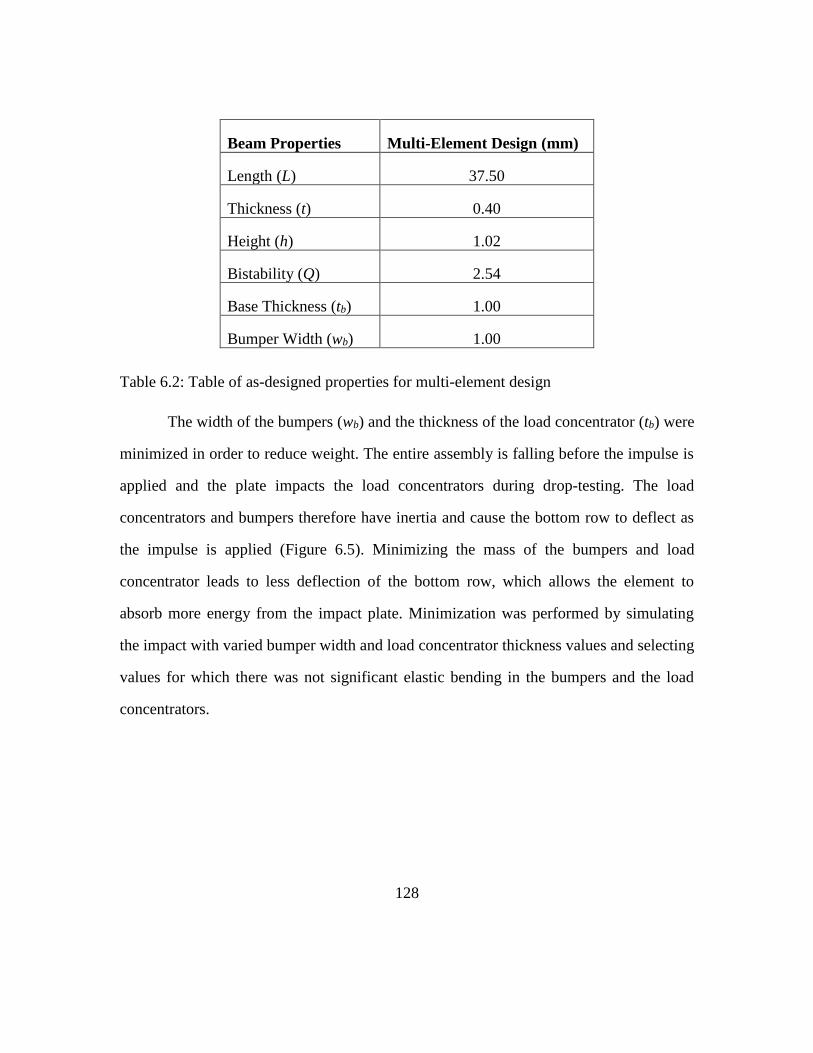
128
Beam Properties Multi-Element Design (mm)
Length (L) 37.50
Thickness (t) 0.40
Height (h) 1.02
Bistability (Q) 2.54
Base Thickness (tb) 1.00
Bumper Width (wb) 1.00
Table 6.2: Table of as-designed properties for multi-element design
The width of the bumpers (wb) and the thickness of the load concentrator (tb) were
minimized in order to reduce weight. The entire assembly is falling before the impulse is
applied and the plate impacts the load concentrators during drop-testing. The load
concentrators and bumpers therefore have inertia and cause the bottom row to deflect as
the impulse is applied (Figure 6.5). Minimizing the mass of the bumpers and load
concentrator leads to less deflection of the bottom row, which allows the element to
absorb more energy from the impact plate. Minimization was performed by simulating
the impact with varied bumper width and load concentrator thickness values and selecting
values for which there was not significant elastic bending in the bumpers and the load
concentrators.
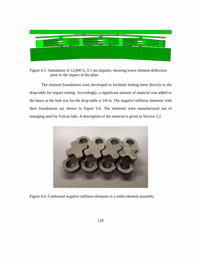
129
Figure 6.5: Simulation of 12,000 G, 0.1 ms impulse, showing lower element deflection
prior to the impact of the plate
The element foundations were developed to facilitate bolting them directly to the
drop-table for impact testing. Accordingly, a significant amount of material was added to
the bases as the bolt size for the drop-table is 3/8 in. The negative stiffness elements with
their foundations are shown in Figure 6.6. The elements were manufactured out of
maraging steel by Vulcan labs. A description of the material is given in Section 5.2.
Figure 6.6: Conformal negative stiffness elements in a multi-element assembly

130
6.2 QUASI-STATIC TESTING OF MULTI-ELEMENT ASSEMBLIES
Test Setup
A 100 kN MTS load frame with bottom spherical self-aligning platen was used
for quasi-static testing (Figure 6.7). The self-aligning platen allowed the load to be
applied nearly orthogonally to the bottom plane of the assembly. The platen was aligned
before testing by carefully compressing the top and bottom platens together so that they
were parallel. After testing it was found that both platens were still parallel. The self-
aligning platen did not move during testing. Except for the self-aligning platen, testing
was conducted in the same manner as in Section 3.3.
Figure 6.7: Image of quasi-static multi-element testing setup with self-aligning platen
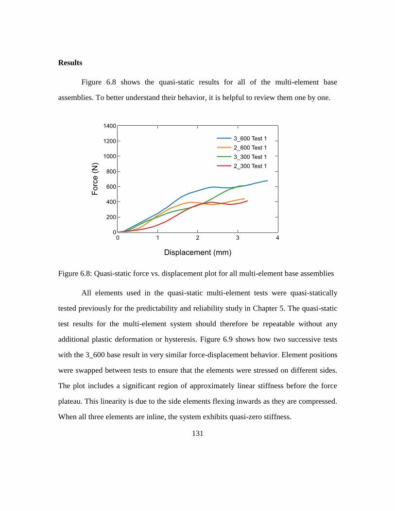
131
Results
Figure 6.8 shows the quasi-static results for all of the multi-element base
assemblies. To better understand their behavior, it is helpful to review them one by one.
Figure 6.8: Quasi-static force vs. displacement plot for all multi-element base assemblies
All elements used in the quasi-static multi-element tests were quasi-statically
tested previously for the predictability and reliability study in Chapter 5. The quasi-static
test results for the multi-element system should therefore be repeatable without any
additional plastic deformation or hysteresis. Figure 6.9 shows how two successive tests
with the 3_600 base result in very similar force-displacement behavior. Element positions
were swapped between tests to ensure that the elements were stressed on different sides.
The plot includes a significant region of approximately linear stiffness before the force
plateau. This linearity is due to the side elements flexing inwards as they are compressed.
When all three elements are inline, the system exhibits quasi-zero stiffness.
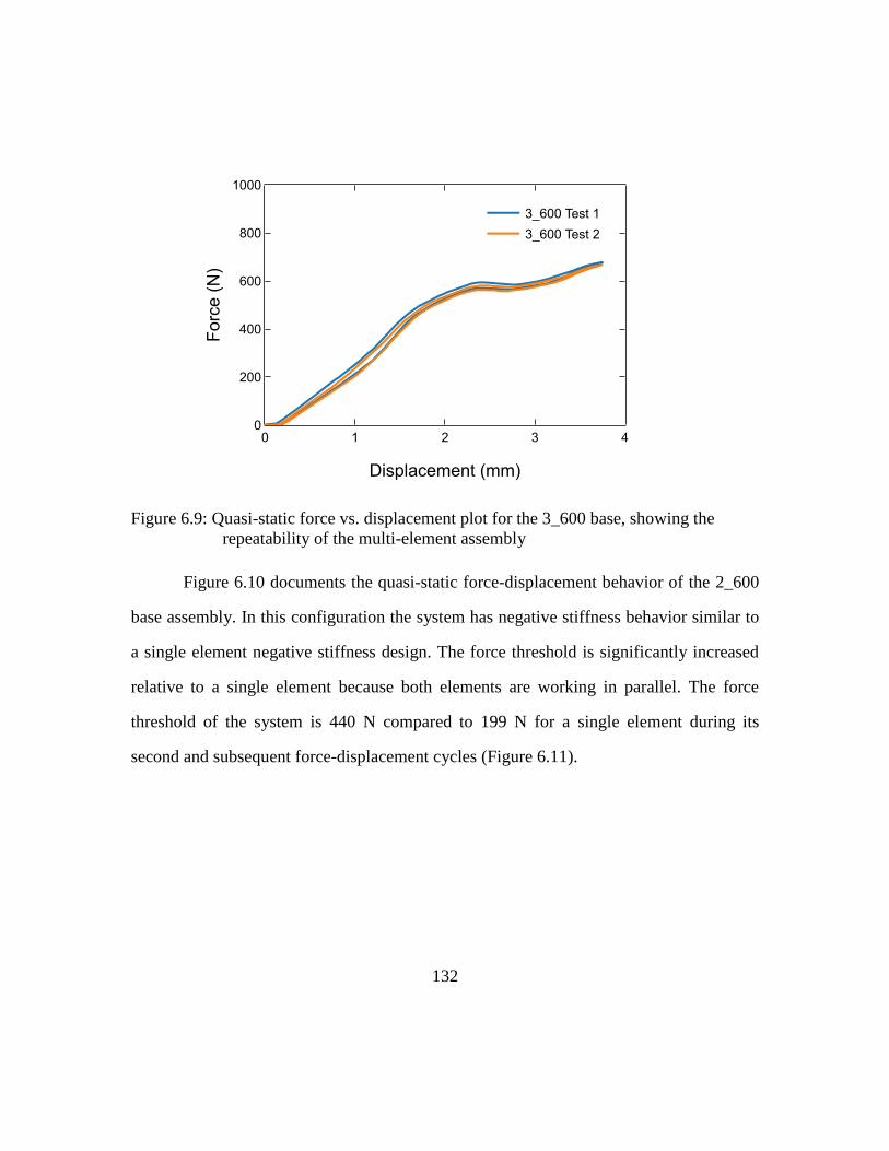
132
Figure 6.9: Quasi-static force vs. displacement plot for the 3_600 base, showing the
repeatability of the multi-element assembly
Figure 6.10 documents the quasi-static force-displacement behavior of the 2_600
base assembly. In this configuration the system has negative stiffness behavior similar to
a single element negative stiffness design. The force threshold is significantly increased
relative to a single element because both elements are working in parallel. The force
threshold of the system is 440 N compared to 199 N for a single element during its
second and subsequent force-displacement cycles (Figure 6.11).
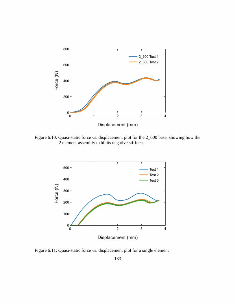
133
Figure 6.10: Quasi-static force vs. displacement plot for the 2_600 base, showing how the
2 element assembly exhibits negative stiffness
Figure 6.11: Quasi-static force vs. displacement plot for a single element
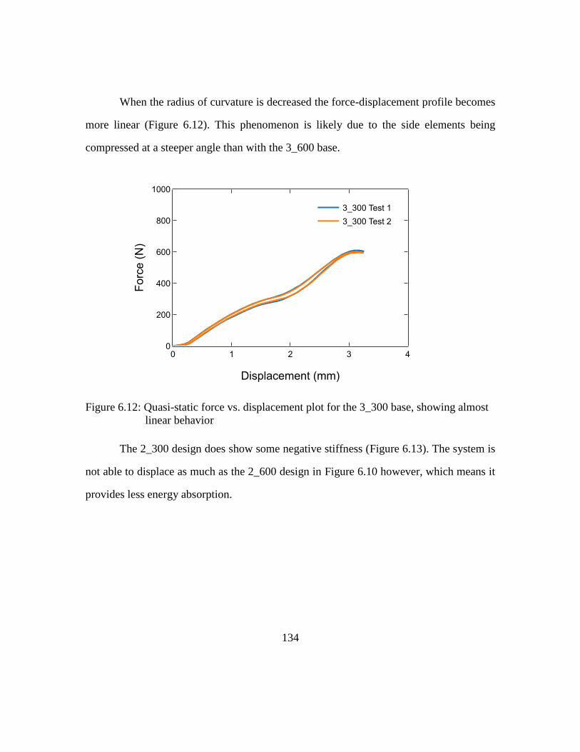
134
When the radius of curvature is decreased the force-displacement profile becomes
more linear (Figure 6.12). This phenomenon is likely due to the side elements being
compressed at a steeper angle than with the 3_600 base.
Figure 6.12: Quasi-static force vs. displacement plot for the 3_300 base, showing almost
linear behavior
The 2_300 design does show some negative stiffness (Figure 6.13). The system is
not able to displace as much as the 2_600 design in Figure 6.10 however, which means it
provides less energy absorption.
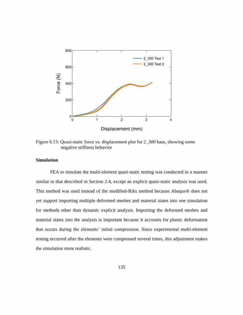
135
Figure 6.13: Quasi-static force vs. displacement plot for 2_300 base, showing some
negative stiffness behavior
Simulation
FEA to simulate the multi-element quasi-static testing was conducted in a manner
similar to that described in Section 2.4, except an explicit quasi-static analysis was used.
This method was used instead of the modified-Riks method because Abaqus® does not
yet support importing multiple deformed meshes and material states into one simulation
for methods other than dynamic explicit analysis. Importing the deformed meshes and
material states into the analysis is important because it accounts for plastic deformation
that occurs during the elements’ initial compression. Since experimental multi-element
testing occurred after the elements were compressed several times, this adjustment makes
the simulation more realistic.
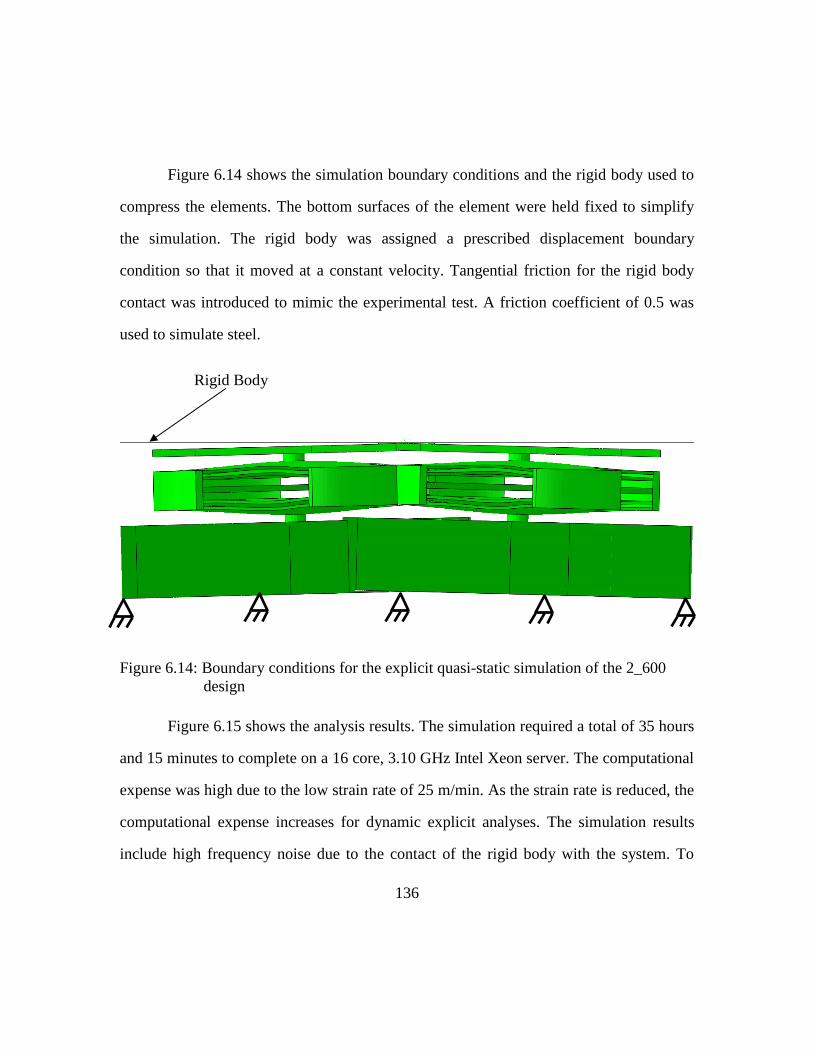
136
Figure 6.14 shows the simulation boundary conditions and the rigid body used to
compress the elements. The bottom surfaces of the element were held fixed to simplify
the simulation. The rigid body was assigned a prescribed displacement boundary
condition so that it moved at a constant velocity. Tangential friction for the rigid body
contact was introduced to mimic the experimental test. A friction coefficient of 0.5 was
used to simulate steel.
Figure 6.14: Boundary conditions for the explicit quasi-static simulation of the 2_600
design
Figure 6.15 shows the analysis results. The simulation required a total of 35 hours
and 15 minutes to complete on a 16 core, 3.10 GHz Intel Xeon server. The computational
expense was high due to the low strain rate of 25 m/min. As the strain rate is reduced, the
computational expense increases for dynamic explicit analyses. The simulation results
include high frequency noise due to the contact of the rigid body with the system. To
Rigid Body
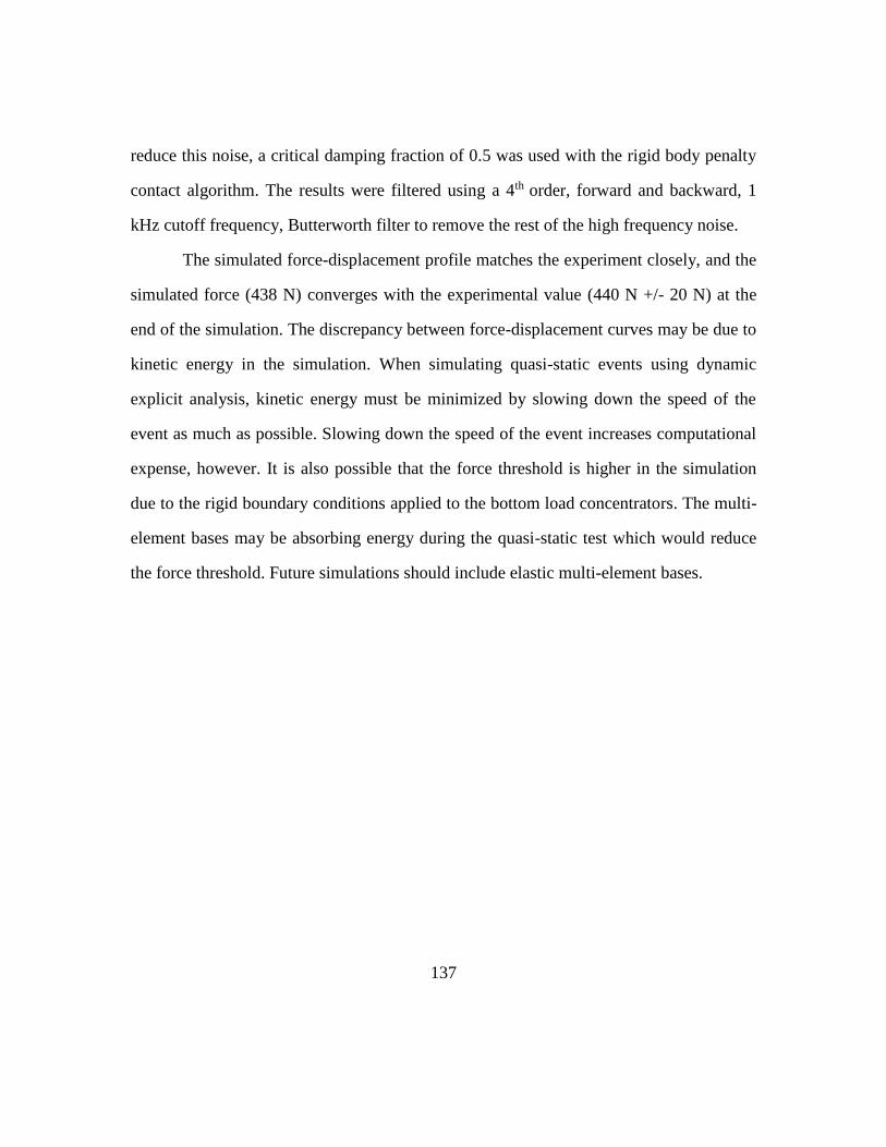
137
reduce this noise, a critical damping fraction of 0.5 was used with the rigid body penalty
contact algorithm. The results were filtered using a 4th order, forward and backward, 1
kHz cutoff frequency, Butterworth filter to remove the rest of the high frequency noise.
The simulated force-displacement profile matches the experiment closely, and the
simulated force (438 N) converges with the experimental value (440 N +/- 20 N) at the
end of the simulation. The discrepancy between force-displacement curves may be due to
kinetic energy in the simulation. When simulating quasi-static events using dynamic
explicit analysis, kinetic energy must be minimized by slowing down the speed of the
event as much as possible. Slowing down the speed of the event increases computational
expense, however. It is also possible that the force threshold is higher in the simulation
due to the rigid boundary conditions applied to the bottom load concentrators. The multi-
element bases may be absorbing energy during the quasi-static test which would reduce
the force threshold. Future simulations should include elastic multi-element bases.
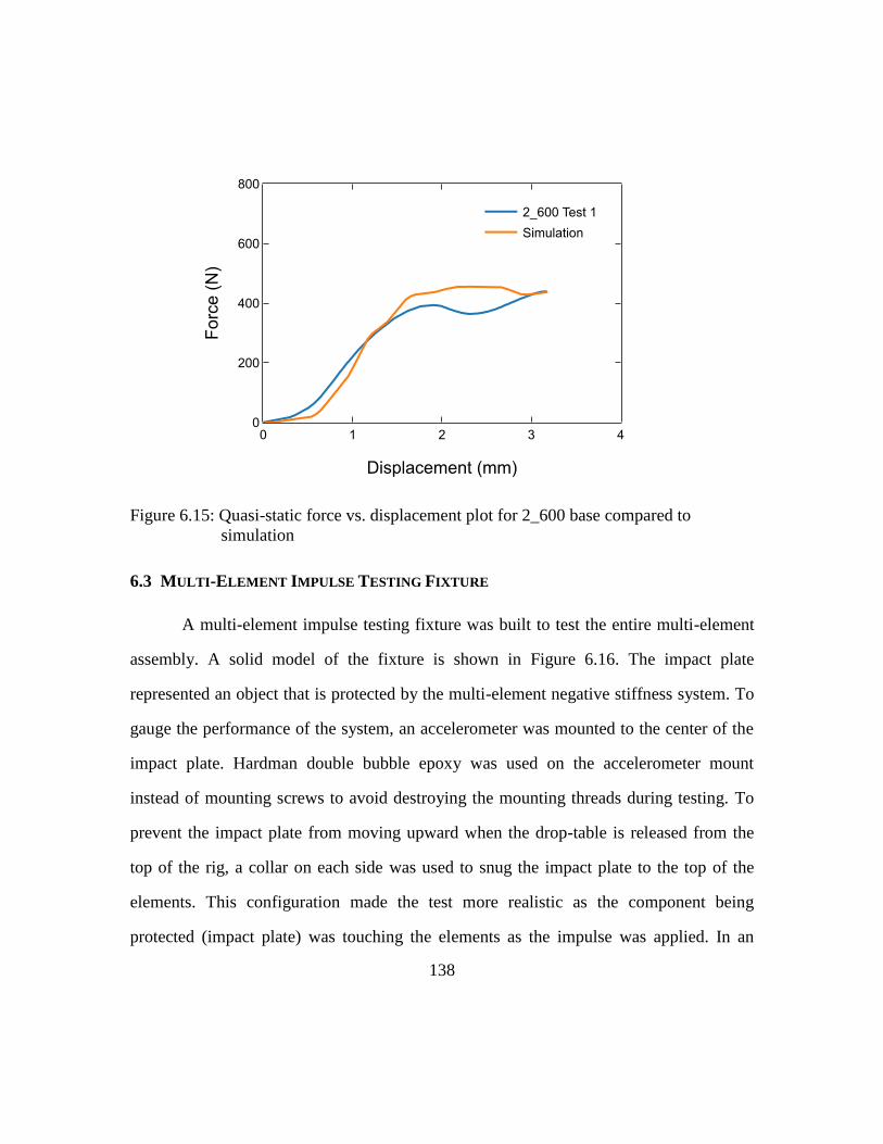
138
Figure 6.15: Quasi-static force vs. displacement plot for 2_600 base compared to
simulation
6.3 MULTI-ELEMENT IMPULSE TESTING FIXTURE
A multi-element impulse testing fixture was built to test the entire multi-element
assembly. A solid model of the fixture is shown in Figure 6.16. The impact plate
represented an object that is protected by the multi-element negative stiffness system. To
gauge the performance of the system, an accelerometer was mounted to the center of the
impact plate. Hardman double bubble epoxy was used on the accelerometer mount
instead of mounting screws to avoid destroying the mounting threads during testing. To
prevent the impact plate from moving upward when the drop-table is released from the
top of the rig, a collar on each side was used to snug the impact plate to the top of the
elements. This configuration made the test more realistic as the component being
protected (impact plate) was touching the elements as the impulse was applied. In an
139
engineering application, the negative stiffness elements would be touching the protected
component.
To simplify the testing, the same multi-element bases used for the quasi-static
testing were used for the impulse testing. The bases bolted to a 12.7 mm (0.5 in) steel
fixture base. The fixture base provided rigidity for the test setup and minimized flexing
on impact. On the sides of the base were two 6.35 mm (0.25 in) threaded steel rods. The
rods allowed the impact plate to move vertically relative to the fixture. The impact plate
moved on high speed linear bearings with ceramic liners. The impact plate was fabricated
from 3.175 mm (0.125 in) hardened 7075 aluminum to reduce weight and add rigidity to
the system. Bearings were attached to the plate using snap rings and aluminum spacers.
The rods were kept in alignment by a top plate made of 6.35 mm (0.25 in) steel. Locknuts
attached to the top threads of the rods to secure them. The fixture was manufactured by
undergraduate researcher Max Garufo.
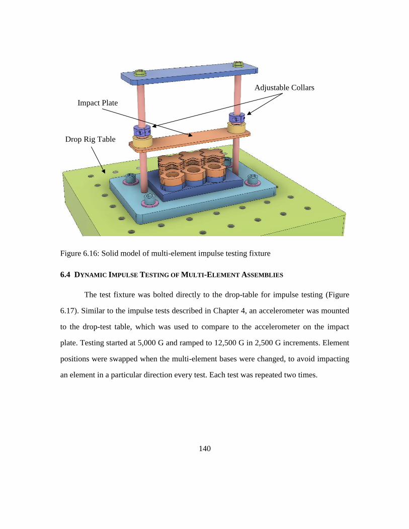
140
Figure 6.16: Solid model of multi-element impulse testing fixture
6.4 DYNAMIC IMPULSE TESTING OF MULTI-ELEMENT ASSEMBLIES
The test fixture was bolted directly to the drop-table for impulse testing (Figure
6.17). Similar to the impulse tests described in Chapter 4, an accelerometer was mounted
to the drop-test table, which was used to compare to the accelerometer on the impact
plate. Testing started at 5,000 G and ramped to 12,500 G in 2,500 G increments. Element
positions were swapped when the multi-element bases were changed, to avoid impacting
an element in a particular direction every test. Each test was repeated two times.
Drop Rig Table
Impact Plate
Adjustable Collars
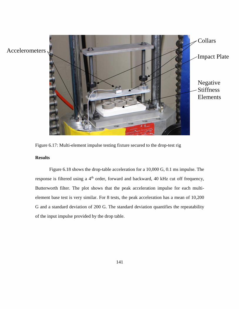
141
Figure 6.17: Multi-element impulse testing fixture secured to the drop-test rig
Results
Figure 6.18 shows the drop-table acceleration for a 10,000 G, 0.1 ms impulse. The
response is filtered using a 4th order, forward and backward, 40 kHz cut off frequency,
Butterworth filter. The plot shows that the peak acceleration impulse for each multi-
element base test is very similar. For 8 tests, the peak acceleration has a mean of 10,200
G and a standard deviation of 200 G. The standard deviation quantifies the repeatability
of the input impulse provided by the drop table.
Accelerometers
Negative
Stiffness
Elements
Impact Plate
Collars
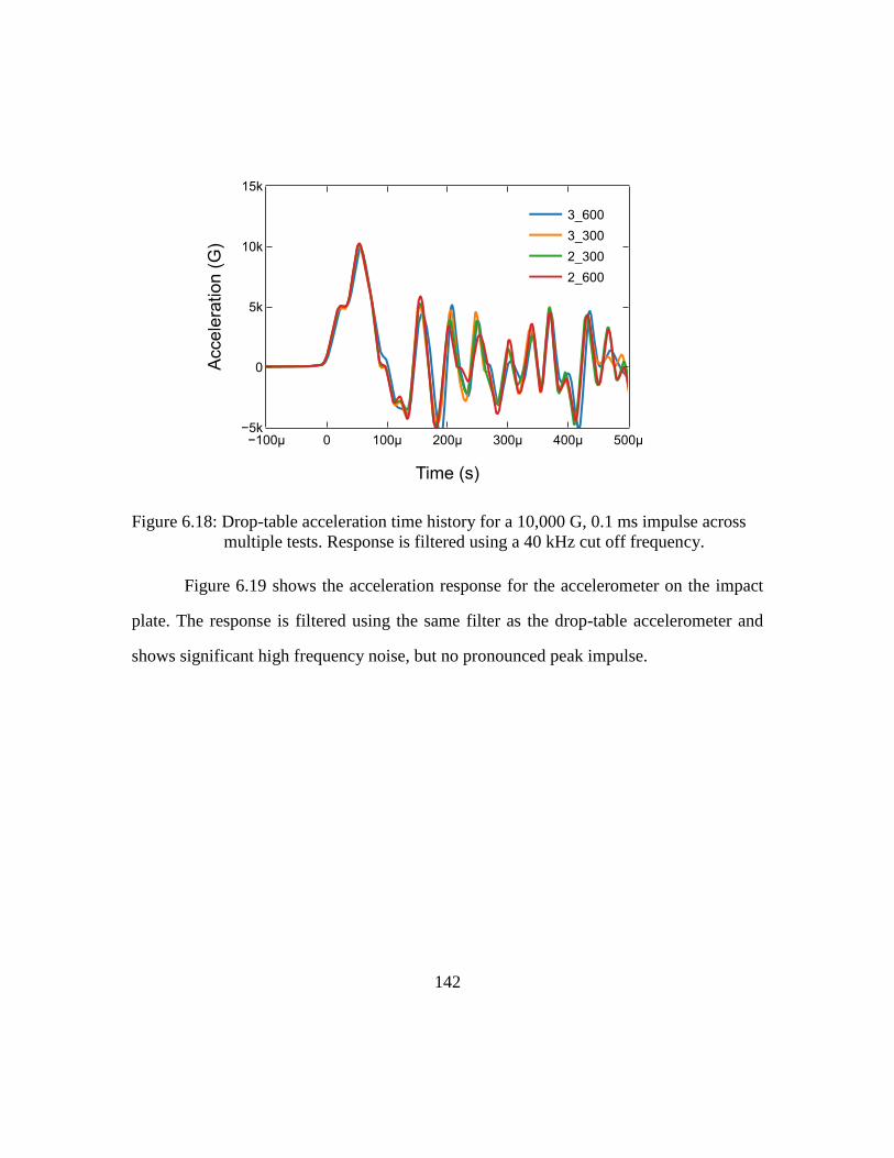
142
Figure 6.18: Drop-table acceleration time history for a 10,000 G, 0.1 ms impulse across
multiple tests. Response is filtered using a 40 kHz cut off frequency.
Figure 6.19 shows the acceleration response for the accelerometer on the impact
plate. The response is filtered using the same filter as the drop-table accelerometer and
shows significant high frequency noise, but no pronounced peak impulse.
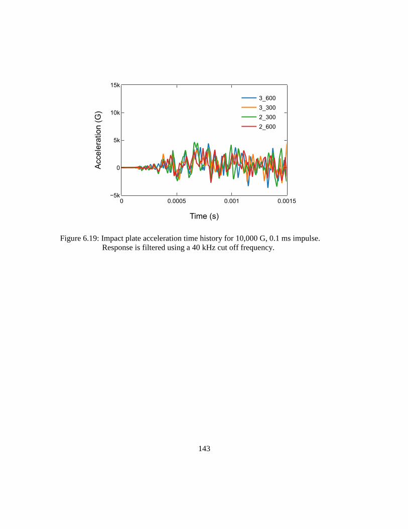
143
Figure 6.19: Impact plate acceleration time history for 10,000 G, 0.1 ms impulse.
Response is filtered using a 40 kHz cut off frequency.
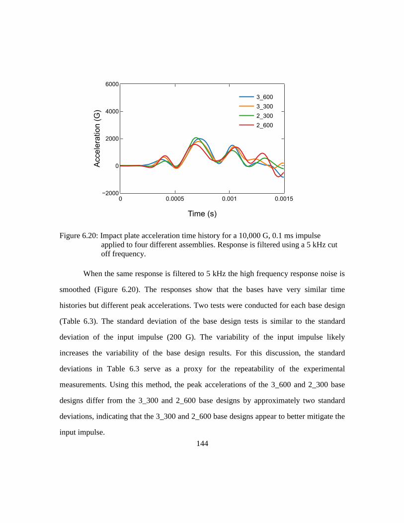
144
Figure 6.20: Impact plate acceleration time history for a 10,000 G, 0.1 ms impulse
applied to four different assemblies. Response is filtered using a 5 kHz cut
off frequency.
When the same response is filtered to 5 kHz the high frequency response noise is
smoothed (Figure 6.20). The responses show that the bases have very similar time
histories but different peak accelerations. Two tests were conducted for each base design
(Table 6.3). The standard deviation of the base design tests is similar to the standard
deviation of the input impulse (200 G). The variability of the input impulse likely
increases the variability of the base design results. For this discussion, the standard
deviations in Table 6.3 serve as a proxy for the repeatability of the experimental
measurements. Using this method, the peak accelerations of the 3_600 and 2_300 base
designs differ from the 3_300 and 2_600 base designs by approximately two standard
deviations, indicating that the 3_300 and 2_600 base designs appear to better mitigate the
input impulse.
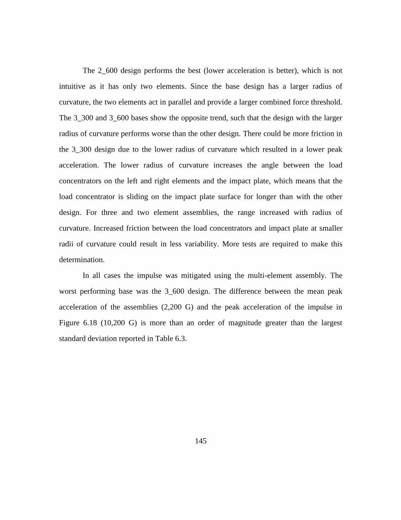
145
The 2_600 design performs the best (lower acceleration is better), which is not
intuitive as it has only two elements. Since the base design has a larger radius of
curvature, the two elements act in parallel and provide a larger combined force threshold.
The 3_300 and 3_600 bases show the opposite trend, such that the design with the larger
radius of curvature performs worse than the other design. There could be more friction in
the 3_300 design due to the lower radius of curvature which resulted in a lower peak
acceleration. The lower radius of curvature increases the angle between the load
concentrators on the left and right elements and the impact plate, which means that the
load concentrator is sliding on the impact plate surface for longer than with the other
design. For three and two element assemblies, the range increased with radius of
curvature. Increased friction between the load concentrators and impact plate at smaller
radii of curvature could result in less variability. More tests are required to make this
determination.
In all cases the impulse was mitigated using the multi-element assembly. The
worst performing base was the 3_600 design. The difference between the mean peak
acceleration of the assemblies (2,200 G) and the peak acceleration of the impulse in
Figure 6.18 (10,200 G) is more than an order of magnitude greater than the largest
standard deviation reported in Table 6.3.
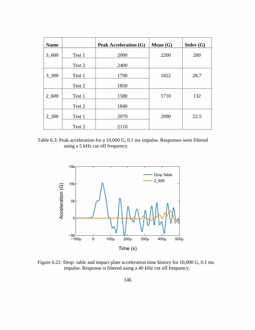
146
Name Peak Acceleration (G) Mean (G) Stdev (G)
3_600 Test 1 2000 2200 200
Test 2 2400
3_300 Test 1 1790 1822 28.7
Test 2 1850
2_600 Test 1 1580 1710 132
Test 2 1840
2_300 Test 1 2070 2090 22.5
Test 2 2110
Table 6.3: Peak acceleration for a 10,000 G, 0.1 ms impulse. Responses were filtered
using a 5 kHz cut off frequency.
Figure 6.21: Drop- table and impact plate acceleration time history for 10,000 G, 0.1 ms
impulse. Response is filtered using a 40 kHz cut off frequency.
147
Simulation
The FEA was conducted using the procedure described in Section 6.2 except the
impact mass was modeled as a 7075 aluminum deformable body with S4R shells, and the
critical dampening fraction was removed. These changes were made to model the flexing
of the impact mass under the impulse loading and to mimic the vibration that results from
this flexing. The impact mass was constrained to move only along the y-axis using the
two holes shown in Figure 6.22. These restrictions mimic the boundary conditions of the
experimental test.
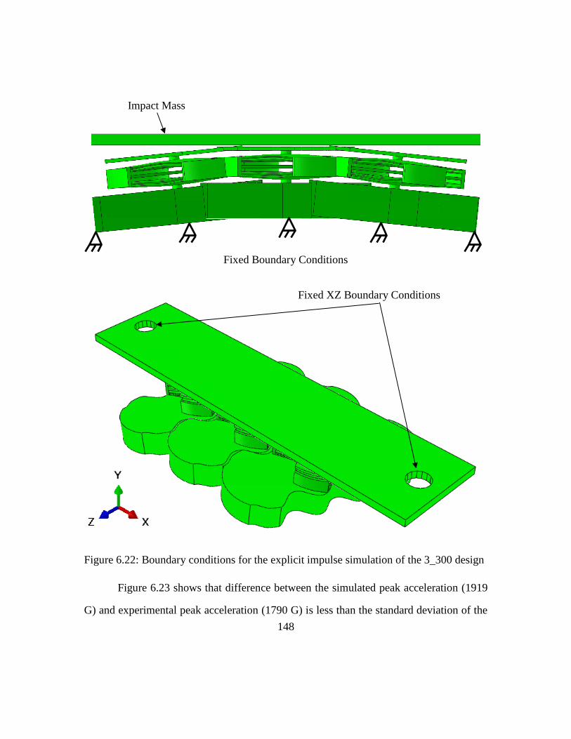
148
Figure 6.22: Boundary conditions for the explicit impulse simulation of the 3_300 design
Figure 6.23 shows that difference between the simulated peak acceleration (1919
G) and experimental peak acceleration (1790 G) is less than the standard deviation of the
Fixed XZ Boundary Conditions
Impact Mass
Fixed Boundary Conditions
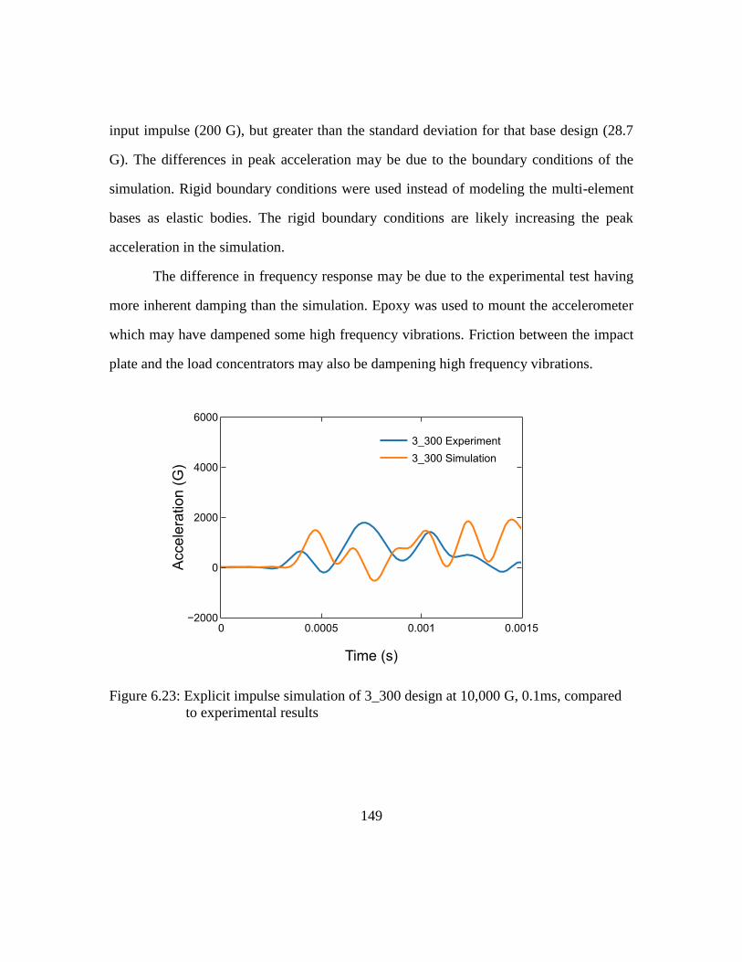
149
input impulse (200 G), but greater than the standard deviation for that base design (28.7
G). The differences in peak acceleration may be due to the boundary conditions of the
simulation. Rigid boundary conditions were used instead of modeling the multi-element
bases as elastic bodies. The rigid boundary conditions are likely increasing the peak
acceleration in the simulation.
The difference in frequency response may be due to the experimental test having
more inherent damping than the simulation. Epoxy was used to mount the accelerometer
which may have dampened some high frequency vibrations. Friction between the impact
plate and the load concentrators may also be dampening high frequency vibrations.
Figure 6.23: Explicit impulse simulation of 3_300 design at 10,000 G, 0.1ms, compared
to experimental results
150
Conclusion
Using negative stiffness elements in a multi-element assembly results in a
reduction of impulse peak acceleration and an increase in impulse duration. This system
could be applied on a large scale to multiple sensitive components. Since these elements
are made of metal, they can survive adverse conditions that other technologies, such as
foam, could not. Since the system is monostable and repeatable it can be used for several
impacts with little to no performance degradation.
151
Conclusion
The main goal of this research is to study the quasi-static and dynamic mechanical
response of negative stiffness elements and to develop the simulation and experimental
framework necessary for them to be implemented in systems requiring mechanical shock
mitigation. Future work is needed to study issues such as fatigue, high frequency noise
and energy dissipation. If these issues are addressed, then negative stiffness elements can
become a more viable alternative to existing technologies.
7.1: RESEARCH CONTRIBUTIONS
A conformal negative stiffness element was designed to protect objects with curved
surfaces.
The first contribution was developing a conformal negative stiffness element that
could be tiled across a curved surface and mitigate impacts that are not perfectly
orthogonal to the load concentrator on the top of the element. While the 2.5D design is
easy to produce using additive or conventional fabrication methods, mechanical loadings
that are not perfect orthogonal to the plane of its load concentrator could damage the
element. The load concentrator and other components in the conformal design flex to
respond to mechanical loads that are not perfectly orthogonal. As shown in Chapter 6, the
force threshold decreases when the force is applied at an angle, but significant levels of
non-orthogonal loading can be accommodated without damage to the element.
152
Quasi-static and dynamic FEA of the two dimensional and conformal elements was
conducted to predict their impact mitigation performance.
A parametric FEA simulation framework was built that allows for rapid design
and optimization of 2.5D and conformal negative stiffness elements. The previous
approach for designing a 2.5D prototype was to build a parametric model of the geometry
in Solidworks and import the CAD file into Abaqus®. Mesh, boundary conditions, and
load were then applied manually in Abaqus®.
All of these steps are automated with the parametric FEA framework. The
designer writes a configuration file with the desired dimensions and executes the
underlying script. The geometry is created and meshed; boundary conditions are applied;
and the resulting model is ready for simulation. The parametric FEA framework is critical
for designing conformal prototypes because it facilitates iterative design and simulation
of an element with greater geometric complexity than the 2.5D design.
Further capabilities of the parametric FEA code include executing multiple
analyses sequentially. For the predictability and reliability study conducted in Chapter 5,
100 analyses were placed in a queue and executed automatically. Automation allows the
designer to work on other tasks while the designs are simulating. The task of generating
stress versus strain curves was also automated. For the predictability and reliability
analysis, the quasi-static stress-strain results from 100 simulations were written to a
JSON file, which could be read easily by a MATLAB® or Python program.
The parametric FEA framework was also organized using industry standard Git
version control. Git not only archives changes to the code, but also allows multiple
engineers to work on the code simultaneously. With hundreds of operations performed by
153
the simulation framework, it is crucial to archive code history and comments with a
version control framework.
Quasi-static and dynamic testing of 2.5D and conformal negative stiffness elements
was conducted to evaluate their impact mitigation performance and compare it with
simulation-based predictions.
Quasi-static testing was conducted on the 2.5D and conformal elements to
evaluate their impact mitigation performance and to evaluate the accuracy of the FEA
framework. Several quasi-static and dynamic experimental trials were conducted with the
2.5D elements to compare elements with the same beam dimensions but different
numbers of columns and rows. Experimental tests showed that increasing the number of
rows has little effect on force threshold, but does increase the amount of energy that can
be absorbed on impact. Experimental tests also showed that increasing the drop height
(and therefore speed) of an impact plate had no effect on the force threshold, but did
cause more energy to be absorbed. Further testing on elements held in a compressed state
versus an uncompressed state showed the impact mitigation potential of the 2.5D design
is primarily due to the architecture of the element rather than the properties of its
constituent material.
Conformal designs were tested quasi-statically to determine if their behavior
would be similar to the 2.5D designs. The nylon conformal designs were shown to exhibit
similar snap-through behavior to the 2.5D designs. One row of the conformal design
snapping through is represented as a blunt serration on the forces versus displacement
plot. The nylon conformal design also exhibited a significant amount of hysteresis due to
the viscoelasticity of the material. The conformal design was also shown analytically to
provide greater force threshold per occupied volume than the 2.5D design.
154
Quasi-static and impact results were compared to FEA simulations to validate the
accuracy of the simulations. The parametric FEA framework was shown to predict force
thresholds and peak accelerations similar to experimental results. For the metal 2.5D
design, the acceleration and time response of an impact was shown to be bounded by
running two different simulations: one simulation with the as-designed dimensions, and
the other with the average as-built dimensions.
Dynamic impulse testing at Sandia National Laboratories was conducted to
investigate the impact mitigation performance of conformal negative stiffness
elements under extremely high acceleration impulses.
High energy, dynamic impulse tests were conducted at Sandia National
Laboratories to investigate the mechanical response of the conformal element.
Experimental tests demonstrated that a metal conformal design could mitigate a 12,000
G, 0.1 ms impulse, and reduce the peak acceleration by an order of magnitude.
Experimental tests also showed that the conformal design lengthens the duration of the
impact mitigation response, compared to an impulse response without the benefit of the
element.
Experimental results were compared to FEA simulations to validate the accuracy
of the simulation results. It was found that the FEA simulations can predict the peak
acceleration of the impulse response to within 3.5% of the experimental result. The time
response does not match well, however, and further work is needed to investigate the
underlying cause. It is possible that the accelerometer moves laterally during the
experimental test which causes the response to differ from the simulation.
155
A predictability and reliability study was conducted to evaluate the effect of various
sources of uncertainty or variability on the impact mitigation performance of
conformal elements.
The DMLS additive manufacturing process introduced variability in geometry
and material properties. Therefore, it was necessary to study its effect on the performance
of the conformal design. The study showed that by incorporating material, beam
thickness, height, and shape imperfection variability into a parametric FEA model, mean
values and standard deviations for force threshold could be obtained. 100 designs
sampled over these sources of variability yielded an estimate of mean force threshold that
differed from the experimental mean by 15 N, which is within the +/- 20 N precision of
the load cell. The predictive accuracy of the model means that it can be used in the future
to predict the force threshold and impact mitigation performance of new designs.
Also, micro CT was used to accurately measure beam thickness across the beam
surface and to map beam shape imperfections onto FEA surfaces. For an experimental
design this information improved the accuracy of FEA results by changing the shape of
the force versus displacement curve such that it was almost entirely bounded by two
experimental results. Using this approach, the beam thickness can be mapped across the
beam surface, which allows the designer to visualize problematic regions where beam
thickness is too low. In the future it may be possible to map an approximation of beam
thicknesses automatically to FEA models so that predictions of quasi-static force versus
displacement behavior are more accurate prior to experimental testing.
156
Multi-element testing was conducted to evaluate the impact mitigation performance
of conformal elements under more realistic conditions.
A multi-element test fixture was designed and built with the help of
undergraduate student Max Garufo. This fixture enabled impact testing of multiple
elements simultaneously in a conformal configuration using the Sandia National
Laboratories drop-test rig. Additively manufactured bases facilitated testing with
different angles between the elements and the mechanical loading and with sets of two or
three elements.
Quasi-static tests showed that the force threshold of the design decreased as the
radius of curvature of the base fixture decreased. The elements on the side were loaded at
a greater angle, which decreased their efficiency in terms of mechanical energy
absorption during the loading portion of the compression cycle. The two element design
generally performed better than the three element design. In the two element
configuration both elements worked in parallel after the compressive loading caused the
load concentrators to rotate into an orientation parallel with the compression platen. The
three element configuration operated similarly, but much greater compressive loads were
required to engage all elements because of the increased angle of the load concentrators
with respect to the compression platen, which decreased the efficiency of the three
element configuration relative to the two element configuration.
Impulse testing showed that more than one element could be engaged
simultaneously to protect a falling object from a severe impulse. A 10,000 G impulse was
reduced to less than 2,500 G for all base designs. The impulse testing rig also withstood
the drop-tests with no damage. This testing showed that there is a potential for using
multiple elements together to protect sensitive components.
157
7.2: FUTURE WORK
This research motivates several opportunities for future work.
Fatigue Testing
Several elements could be compressed cyclically using a load frame in order to
investigate changes in force threshold with the total number of loading cycles. Elements
could also be tested to failure to determine the total number of cycles to failure. Both
quasi-static and dynamic fatigue testing is needed. A failure analysis could be conducted
to identify how the element failed and identify possible design changes.
Investigate Build Orientation
Anisotropic material properties inherent with the DMLS process may be affecting
the dynamic response of the negative stiffness honeycombs. A study should be conducted
that characterizes the dynamic response of honeycombs built with different build
orientations. Impulse testing could be conducted with the peak acceleration and
frequency of oscillation recorded.
Adding Damping Material
The impulse tests on the conformal design indicated significant high frequency
noise during the impact tests, as measured by the accelerometer. Experiments are needed
to investigate the sources of this noise, and design changes may be needed to reduce it.
Possible avenues include adding damping material to the accelerometer mount, if the
noise is caused by inadequate adhesion of the accelerometer to the elements, or adding
damping material to the element mounting surface or the element itself.
158
Metal Conformal Design Energy Dissipation
When the metal designs are exposed to a severe impulse, they excel at mitigating
the impulse, but many compression cycles are required for complete dissipation of the
energy absorbed. The nylon honeycombs absorb more energy because of the
viscoelasticity of the material, so possible ways to dampen the metal honeycombs include
coating the beams with a viscoelastic material. Friction could also be incorporated into
the downward movement of the design. The DMLS process produces a rough surface
finish that is hardened by heat treatments. Surfaces could be rubbed together to dissipate
energy. Alternatively, traditional damping techniques such as air dampers could be
incorporated into the design additively. These designs would push air through an orifice
as the beams snap through which would dissipate energy.
Negative Stiffness Designs for Helmets
Research has been conducted on negative stiffness elements for personal
protective equipment such as baseball or football helmets. So far this research has
included only elements fabricated from nylon [34] [45] [46], but future work could
include using metal designs to increase the force threshold per given volume, resist
fatigue cracking, and enable better protection. While a fatigue study has not been
conducted on the metal elements, no elements have failed (except for the initial batch of
elements which were fabricated improperly). Metal elements have withstood tens of
compressions without failure. Metal elements could be combined with foam padding or
other forms of damping to increase comfort. Metal elements also have the advantage of
withstanding elevated temperatures, whereas the yield strength of nylon decreases
significantly as it warms [34].
159
References
[1] D. V. Balandin, N. N. Bolotnik and W. D. Pilkey, Optimal protection from impact,
shock and vibration, CRC Press, 2001.
[2] L. J. Gibson and M. F. Ashby, Cellular solids: structure and properties, Cambridge
University Press, 1999.
[3] S. D. Papka and S. Kyriakides, "In-plane compressive response and crushing of
honeycomb," Journal of the Mechanics and Physics of Solids, vol. 42, pp. 1499-
1532, 1994.
[4] A. M. Hayes, A. Wang, B. M. Dempsey and D. L. McDowell, "Mechanics of linear
cellular alloys," Mechanics of Materials, vol. 36, pp. 691-713, 2004.
[5] D. M. Correa, T. Klatt, S. Cortes, M. Haberman, D. Kovar and C. Seepersad,
"Negative stiffness honeycombs for recoverable shock isolation," Rapid Prototyping
Journal, vol. 21, pp. 193-200, 2015.
[6] D. M. Correa, C. C. Seepersad and M. R. Haberman, "Mechanical design of negative
stiffness honeycomb materials," Integrating Materials and Manufacturing
Innovation, vol. 4, p. 10, 2015.
[7] D. A. Debeau, C. C. Seepersad and M. R. Haberman, "Impact behavior of negative
stiffness honeycomb materials," Journal of Materials Research, vol. 33, pp. 290-
299, 2018.
[8] C. S. Ha, R. S. Lakes and M. E. Plesha, "Design, fabrication, and analysis of lattice
exhibiting energy absorption via snap-through behavior," Materials & Design, vol.
141, pp. 426-437, 2018.
160
[9] S. Shan, S. H. Kang, J. R. Raney, P. Wang, L. Fang, F. Candido, J. A. Lewis and K.
Bertoldi, "Multistable architected materials for trapping elastic strain energy,"
Advanced Materials, vol. 27, pp. 4296-4301, 2015.
[10] M. E. Pontecorvo, S. Barbarino, G. J. Murray and F. S. Gandhi, "Bistable arches for
morphing applications," Journal of Intelligent Material Systems and Structures, vol.
24, pp. 274-286, 2013.
[11] B. Haghpanah, L. Salari-Sharif, P. Pourrajab, J. Hopkins and L. Valdevit,
"Multistable shape-reconfigurable architected materials," Advanced Materials, vol.
28, pp. 7915-7920, 2016.
[12] T. A. M. Hewage, K. L. Alderson, A. Alderson and F. Scarpa, "Double-negative
mechanical metamaterials displaying simultaneous negative stiffness and negative
poisson's ratio properties," Advanced Materials, vol. 28, pp. 10323-10332, 2016.
[13] T. A. Schaedler, A. J. Jacobsen, A. Torrents, A. E. Sorensen, J. Lian, J. R. Greer, L.
Valdevit and W. B. Carter, "Ultralight metallic microlattices," Science, vol. 334, pp.
962-965, 2011.
[14] X. Zheng, H. Lee, T. H. Weisgraber, M. Shusteff, J. DeOtte, E. B. Duoss, J. D.
Kuntz, M. M. Biener, Q. Ge, J. A. Jackson and others, "Ultralight, ultrastiff
mechanical metamaterials," Science, vol. 344, pp. 1373-1377, 2014.
[15] E. B. Duoss, T. H. Weisgraber, K. Hearon, C. Zhu, W. Small, T. R. Metz, J. J.
Vericella, H. D. Barth, J. D. Kuntz, R. S. Maxwell and others, "Three-dimensional
printing of elastomeric, cellular architectures with negative stiffness," Advanced
Functional Materials, vol. 24, pp. 4905-4913, 2014.
161
[16] A. Rafsanjani, A. Akbarzadeh and D. Pasini, "Snapping mechanical metamaterials
under tension," Advanced Materials, vol. 27, pp. 5931-5935, 2015.
[17] J. Qiu, J. H. Lang and A. H. Slocum, "A curved-beam bistable mechanism," Journal
of Microelectromechanical Systems, vol. 13, pp. 137-146, 2004.
[18] K. Che, C. Yuan, J. Wu, H. J. Qi and J. Meaud, "Three-dimensional-printed
multistable mechanical metamaterials with a deterministic deformation sequence,"
Journal of Applied Mechanics, vol. 84, p. 011004, 2017.
[19] T. Frenzel, C. Findeisen, M. Kadic, P. Gumbsch and M. Wegener, "Tailored
buckling microlattices as reusable light-weight shock absorbers," Advanced
Materials, vol. 28, pp. 5865-5870, 2016.
[20] D. Restrepo, N. D. Mankame and P. D. Zavattieri, "Phase transforming cellular
materials," Extreme Mechanics Letters, vol. 4, pp. 52-60, 2015.
[21] C. Findeisen, J. Hohe, M. Kadic and P. Gumbsch, "Characteristics of mechanical
metamaterials based on buckling elements," Journal of the Mechanics and Physics
of Solids, vol. 102, pp. 151-164, 2017.
[22] Q. Chen, X. Zhang and B. Zhu, "Design of buckling-induced mechanical
metamaterials for energy absorption using topology optimization," Structural and
Multidisciplinary Optimization, vol. 58, pp. 1395-1410, 2018.
[23] A. G. Izard, R. F. Alfonso, G. McKnight and L. Valdevit, "Optimal design of a
cellular material encompassing negative stiffness elements for unique combinations
of stiffness and elastic hysteresis," Materials & Design, vol. 135, pp. 37-50, 2017.
[24] D. A. Debeau and C. C. Seepersad, "Additively manufactured conformal negative
162
stiffness honeycombs," in Proceedings of the Solid Freeform Fabrication
Symposium. The University of Texas at Austin, Austin, TX, 2017.
[25] D. Leigh, "A comparison of polyamide 11 mechanical properties between laser
sintering and traditional molding," in Proceedings of the Solid Freeform Fabrication
Symposium. The University of Texas at Austin, Austin, TX, 2012.
[26] D. L. Bourell, T. J. Watt, D. K. Leigh and B. Fulcher, "Performance limitations in
polymer laser sintering," Physics Procedia, vol. 56, pp. 147-156, 2014.
[27] M. Crisfield, "A fast incremental/iterative solution procedure that handles “snap-
through”," in Computational Methods in Nonlinear Structural and Solid Mechanics,
Elsevier, 1981, pp. 55-62.
[28] ASTM International, "ASTM F2971-13, Standard practice for reporting data for test
specimens prepared by additive manufacturing," 2013. [Online]. Available:
http://www.astm.org/cgi-bin/resolver.cgi?F2971-13.
[29] J. Allison, C. Sharpe and C. C. Seepersad, "A test part for evaluating the accuracy
and resolution of a polymer powder bed fusion process," Journal of Mechanical
Design, vol. 139, no. 10, p. 100902, 2017.
[30] MTS Systems Corporation, "661.11 Force transducer," Eden Prairie, 1996.
[31] G. E. Dieter, "Mechanical Metallurgy," New York, McGraw-Hill, 1986, pp. 434-
438.
[32] J. Zhang, M. Gungor and E. Lavernia, "The effect of porosity on the microstructural
damping response of 6061 aluminium alloy," Journal of Materials Science, vol. 28,
no. 6, pp. 1515-1524, 1993.
163
[33] B. L. Boyce, B. C. Salzbrenner, J. M. Rodelas, L. P. Swiler, J. D. Madison, B. H.
Jared and Y.-L. Shen, "Extreme-value statistics reveal rare failure-critical defects in
additive manufacturing," Advanced Engineering Materials, vol. 19, p. 1700102,
2017.
[34] D. M. Correa, "Design and evaluation of negative stiffness honeycombs for
recoverable shock isolation," M.S. thesis, ME Dept., UT Austin, TX, 2015.
[35] M. Shellabear and O. Nyrhilä, "DMLS-development history and state of the art,"
Laser Assisted Netshape Engineering 4, Proceedings of the 4th LANE, pp. 21-24,
2004.
[36] A. Hussein, L. Hao, C. Yan, R. Everson and P. Young, "Advanced lattice support
structures for metal additive manufacturing," Journal of Materials Processing
Technology, vol. 213, pp. 1019-1026, 2013.
[37] B. Vandenbroucke and J.-P. Kruth, "Selective laser melting of biocompatible metals
for rapid manufacturing of medical parts," Rapid Prototyping Journal, vol. 13, pp.
196-203, 2007.
[38] S. Das, J. J. Beama, M. Wohlert and D. L. Bourell, "Direct laser freeform fabrication
of high performance metal components," Rapid Prototyping Journal, vol. 4, pp. 112-
117, 1998.
[39] B. C. Salzbrenner, J. M. Rodelas, J. D. Madison, B. H. Jared, L. P. Swiler, Y.-L.
Shen and B. L. Boyce, "High-throughput stochastic tensile performance of
additively manufactured stainless steel," Journal of Materials Processing
Technology, vol. 241, pp. 1-12, 2017.
164
[40] ASTM International, "ASTM E8 / E8M-16a, Standard test methods for tension
testing of metallic materials," 2016. [Online]. Available: http://www.astm.org/cgi-
bin/resolver.cgi?E8E8M-16a.
[41] Renishaw, "Maraging steel M300 powder for additive manufacturing," July 2017.
[Online]. Available: https://www.renishaw.com/additive.
[42] S. Holcombe, "splitFV - split a mesh," 24 June 2014. [Online]. Available:
https://www.mathworks.com/matlabcentral/fileexchange/27667-splitfv-split-a-mesh.
[43] M. D. McKay, R. J. Beckman and W. J. Conover, "Comparison of three methods for
selecting values of input variables in the analysis of output from a computer code,"
Technometrics, vol. 21, pp. 239-245, 1979.
[44] J. C. Helton and F. J. Davis, "Latin hypercube sampling and the propagation of
uncertainty in analyses of complex systems," Reliability Engineering & System
Safety, vol. 81, pp. 23-69, 2003.
[45] P. Alok, "Application of additively manufactured conformal negative stiffness
honeycombs for impact isolation in protective headgear," M.S. thesis, ME Dept., UT
Austin, TX, 2018.
[46] Z. Ahmed, "Negative stiffness elements for helmet padding application," ME 377K
Report, ME Dept., UT Austin, TX, 2018.