Embed Size (px)
Citation preview

latrobe.edu.au
CRICOS Provider 00115M
CRICOS Provider 00115M
What does radical price change and choice
reveal?
A project by Yarra Valley Water and the Centre for Water
Policy Management
November 2016

2La Trobe University
Objectives
� The aim is to estimate the price elasticity of demand for
residential water in Melbourne (serviced by Yarra Valley Water).
No previous estimates in Melbourne
Previous research indicates elasticity estimates vary by location
� Timing of the study.
In 2013 – July 1 prices increased by 21.7% + CPI (see YVW Annual
report 2013-14).
This comes after a two year period of no price increases, so provides a
unique opportunity to estimate consumer's response.
Also attitudinal survey provided an opportunity to estimate the
elasticity controlling for a number of household characteristics.
3La Trobe University
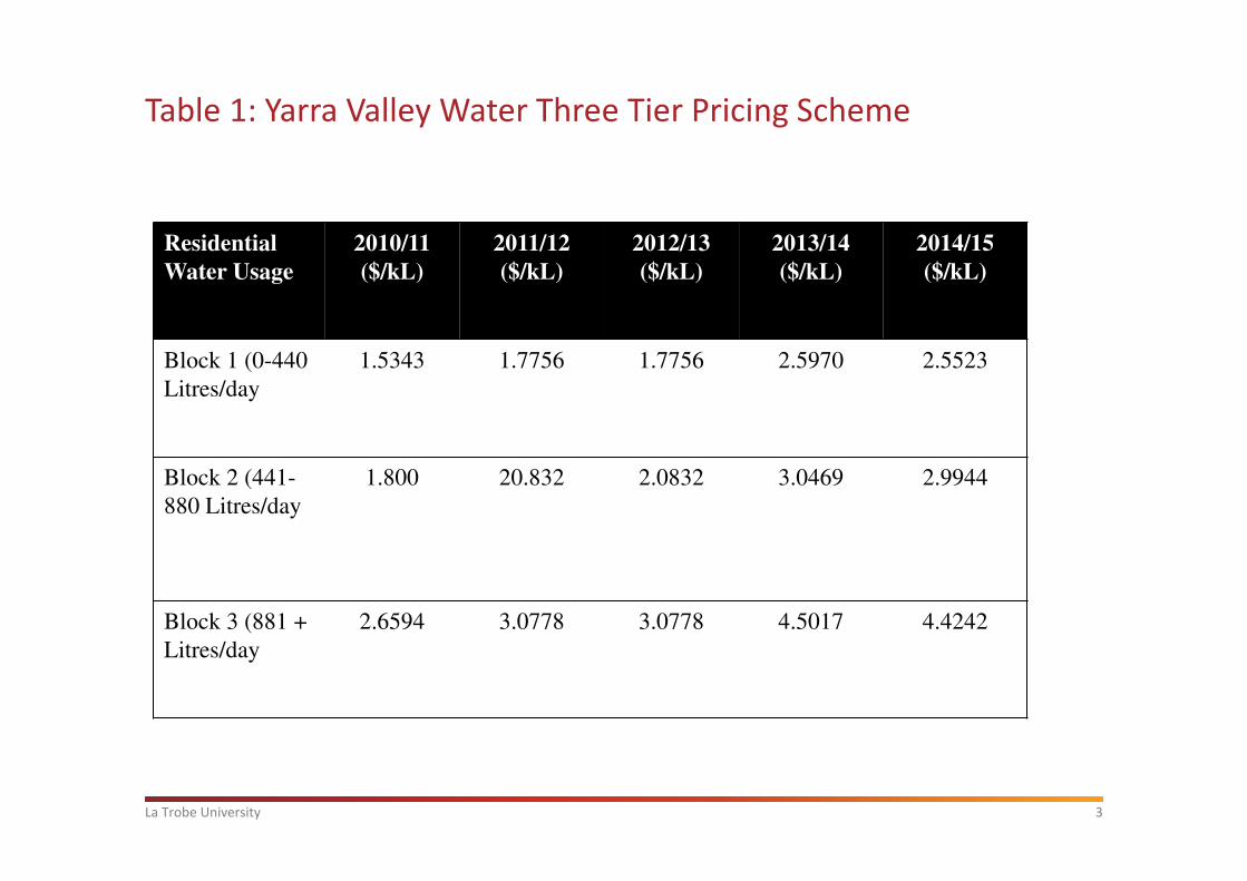
Table 1: Yarra Valley Water Three Tier Pricing Scheme
Residential
Water Usage
2010/11
($/kL)
2011/12
($/kL)
2012/13
($/kL)
2013/14
($/kL)
2014/15
($/kL)
Block 1 (0-440
Litres/day
1.5343 1.7756 1.7756 2.5970 2.5523
Block 2 (441-
880 Litres/day
1.800 20.832 2.0832 3.0469 2.9944
Block 3 (881 +
Litres/day
2.6594 3.0778 3.0778 4.5017 4.4242

4La Trobe University
Previous literature
� Previous estimates of the price elasticity of demand indicate an
inelastic demand for water.
� Meta analysis:
Dalhuisen et al. (2003) report a mean price elasticity mean of -0.41 and
median of -0.35 - SD of 0.81(124 studies)
Sebri (2014) report a mean of -more recent study finds -0.365 and a
median of -0.291 (100 studies)
� Key factors affecting demand and included in studies are the
pricing structure, income, rainfall, temperature, household size
and property size.

5La Trobe University
Table 2: Estimated price elasticities in Australia
Author(s) Data Location Price Elasticity Method Function
Hoffman,
Worthington and
Higgs (2006)
Panel Brisbane SR -0.588
LR -1.16
OLS Linear
and log-
log
Grafton and
Kompas (2007)
Panel Sydney -0.352 OLS Linear
Grafton and Ward
(2008)
Aggregate Sydney -0.17 OLS Linear
Abrams, Sarafidis,
Kumaradevan and
Spaninks (2012)
Panel Sydney SR -0.082
LR -0.139
GMM Log-
linear
ICRC (2016) Panel ACT -0.14 2SLS Log-log
YVW and CWPM Panel Melbourne -0.09 to -0.3 OLS,
GMM, FE
and FD
Linear
and log-
linear
6La Trobe University
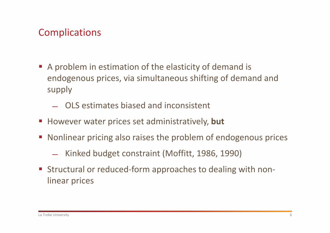
Complications
� A problem in estimation of the elasticity of demand is
endogenous prices, via simultaneous shifting of demand and
supply
OLS estimates biased and inconsistent
� However water prices set administratively, but
� Nonlinear pricing also raises the problem of endogenous prices
Kinked budget constraint (Moffitt, 1986, 1990)
� Structural or reduced-form approaches to dealing with non-
linear prices

7La Trobe University
Figure 1 Budget constraint with nonlinear pricing
I3
I2
I1
QX
QWQK

8La Trobe University
Complications
� A second estimation issue with nonlinear pricing is what price
to use; marginal, average prices, both and also a difference
variable (Nordin 1976)
� This has been debated in the literature and relates to water
pricing, electricity and income tax rates (see Shin 1985,
Nieswiadowy and Monila 1991)
� A recent study (Ito 2014) on nonlinear electricity prices argues
that consumers respond to average rather than marginal prices
The implication is that nonlinear pricing does no have the
desired impact on energy conservation

9La Trobe University
Econometric method
� Based on the data and potential problems in estimation we
used several econometric techniques
� Pooled OLS:
Likely to be biased and inconsistent
But estimates the effects of household characteristics
� Fixed effects and a first difference model
These models remove the household heterogeneity.
More likely to be unbiased and consistent estimates.
� GMM model (Arellano Bond) uses lagged consumption as an
instrumental variable to correct for endogeneity

10La Trobe University
Methods
� Functional form of model:
A linear function
A log-linear function – typically the preferred form in water demand
studies
� Using the survey data to form a panel (unbalanced):
Average price (with 3 lags), household income, household size split
into adults and children, rainfall per quarter (in ml) and average
temperature (quarter), lagged consumption and a summer dummy.
Additional household characteristics – swimming pool, rainwater tank,
drip watering system, garden size, vegetable garden and evaporative
cooling.

11La Trobe University
Data
� The data:
Benchmark survey 949 respondents, after dropping outliers and
missing data finished with a panel of 715 households over 16 quarters
from Q3 2011 to Q2 2015.
Average price = estimated Billed amount / Billed usage (We re-
constructed the billed amount or total cost from usage data)
Also modelling the change in marginal price
� Other variables included
Same variables were not significant e.g. outdoor spa and information
on tap type, washing machine, Net Annual Value.

12La Trobe University
Figure 2 Quarterly mean usage (Kl)
0
10
20
30
40
50
60
01-J
ul-
11
01-S
ep-1
1
01-N
ov-1
1
01-J
an-1
2
01-M
ar-1
2
01-M
ay-1
2
01-J
ul-
12
01-S
ep-1
2
01-N
ov-1
2
01-J
an-1
3
01-M
ar-1
3
01-M
ay-1
3
01-J
ul-
13
01-S
ep-1
3
01-N
ov-1
3
01-J
an-1
4
01-M
ar-1
4
01-M
ay-1
4
01-J
ul-
14
01-S
ep-1
4
01-N
ov-1
4
01-J
an-1
5
01-M
ar-1
5
Mea
n U
sag
e K
l
Aggregate mean usage by Quarter (Kl)

13La Trobe University
Figure 3 Average temperature and rainfall by quarter
0
50
100
150
200
250
300
350
400
0
5
10
15
20
25
30
35
01
-Ju
l-1
1
01
-Se
p-1
1
01
-No
v-1
1
01
-Ja
n-1
2
01
-Ma
r-1
2
01
-Ma
y-1
2
01
-Ju
l-1
2
01
-Se
p-1
2
01
-No
v-1
2
01
-Ja
n-1
3
01
-Ma
r-1
3
01
-Ma
y-1
3
01
-Ju
l-1
3
01
-Se
p-1
3
01
-No
v-1
3
01
-Ja
n-1
4
01
-Ma
r-1
4
01
-Ma
y-1
4
01
-Ju
l-1
4
01
-Se
p-1
4
01
-No
v-1
4
01
-Ja
n-1
5
01
-Ma
r-1
5
ml p
er
qu
art
er
C°
Average Temperature Rainfall

14La Trobe University
Figure 4 Quarterly demand for residential water
05
01
00
15
0
Ave
rag
e P
rice
$/K
l
0 100 200 300 400Billed Usage Kl/Quarter

15La Trobe University
05
01
00
15
0A
ve
rag
e P
rice
$/K
l
0 2 4 6Log of Billed Usage
Figure 5 Quarterly demand for residential water (log of usage)

16La Trobe University
Results
� Pooled OLS estimator (similar model to Hoffman et a. 2006)
This was modelled with a lagged dependent variable
Variables not significant and dropped included outdoor spa and
information on tap type, washing machine type, dual flush toilet.
Essentially not enough variation in the data.
White test provides evidence of heteroskadiscitiy
� Linear vs log-linear
Log-linear has higher R2 compared to linear model.
Coefficients generally have the correct sign.
The price variables are significant often to two lags.
Some of the lagged price variables are positive, which is more the
nature of lags – e.g. change in seasons.

17La Trobe University
Results – Model comparisons (linear v log-linear)
Model (1) Model (2) Model (3) Model (4)
Linear levels
Average price
Linear levels
∆Marginal price
Log-linear
Average price
Log-linear
∆Marginal price
Lag of Usage 0.619*** 0.575*** 0.710*** 0.669***
Price -0.586*** -4.671*** -0.0349*** -0.157***
Price 1 lag 0.238*** 0.909* 0.0223*** 0.0564***
Price 2 lags 0.0333 -1.371*** -0.000253 -0.0144*
Price 3 lags -0.0851 -2.688*** -0.000443 -0.0529***
Income 0.258 0 .176 0.00487* 0.00429
Rainwater Tank -1.060 -1.132* -0.00942 -0.0189
Swimming Pool 4.840*** 4.164*** 0.0599*** 0.0477**
Garden size 1.816*** 1.945*** 0.0195** 0.0224***
Vegetable Garden 1.006 0.800 0.0216* 0.0208*
Drip Watering System 3.216*** 3.492*** 0.0450*** 0.0534***
Evaporative cooler 0.782 -0.107 0.0228** 0.00147
Number of Adults 3.823*** 2.703*** 0.0717*** 0.0558***
Number of Children 1.598*** 0.714** 0.0371*** 0.0244***
Average Max Temperature 1.038*** 0.496*** 0.0222*** 0.00924***
Rainfall 0.0384*** 0.0165* 0.000767*** 0.000415**
Summer D 6.742*** 11.41*** 0.0924*** 0.252***
Constant -33.21*** -5.130 0.139* 0.777***
N 6310 6310 6310 6310
Adj-R-Squared 0.586 0.597 0.790 0.746

18La Trobe University
Results
� Elasticities
The price elasticities range from -0.3 to -0.13 suggesting inelastic
demand in line with other studies. This suggests that a 10 per cent
increase in price leads to a 3 per cent reduction in usage.
Household size is an important determinant of water usage more so
than income, which was only significant at the 10% level in one of the
model runs.

19La Trobe University
Results – Elasticities (Model comparisons)
Model (1) Model (2) Model (3) Model (4)
Linear levels
Average price
Linear levels
∆Marginal
price
Log-linear
Average price
Log-linear
∆Marginal
price
Price -0.1308 -0.1661 -0.3129 -0.2236
Price1lag 0.0532 0.3233 0.2002 0.0804
Price2lag 0.0074 -0.0487 -0.0022 -0.0205
Price3lag -0.0190 -0.0956 -0.0039 -0.0755
Income 0.0230 0.0158 0.0050 0.0044
Number of Adults 0.1928 0.1363 0.0416 0.0324
Number of
Children
0.0369 0.0164 0.0098 0.0064

20La Trobe University
Results: Estimators comparison
Model (1)
Pooled OLS
Model (2)
Fixed Effects
Model (3)
First Differences
Model (4)
GMM
Lagged usage 0.710*** 0.193***
AvPrice -0.0349*** -0.0368*** -0.0346*** -0.0316***
AvPrice1lag 0.0223*** -0.00528*** -0.00128 0.00714***
AvPrice2lag -0.000253 -0.000596 0.00109 0.00171
AvPrice3lag -0.000443 0.000239 0.00236** 0.000520
Income 0.00487* 0.750***
Rainwater Tank -0.00942
Swimming Pool 0.0599***
Garden size 0.0195**
Vegetable Garden 0.0216*
Drip Watering System 0.0450***
Evaporative cooler 0.0228**
Number of Adults 0.0717***
Number of Children 0.0371***
Rainfall 0.000767*** 0.000290* 0.00148*** 0.000709***
Av Max Temperature 0.0222*** 0.00370* 0.0123*** 0.00998***
Summer D 0.0924*** 0.179*** 0.147*** 0.162***
Constant 0.139* 3.746***
N 6310 6310 5816 5816
Adj-R-squared 0.790 0.370
Rho 0.7624

21La Trobe University
Results – estimators comparisons
� Different estimators
The fixed effects model – washes out the household heterogeneity and
estimates time varying parameters.
The parameter rho – indicates 76 per cent of variation is due to
household specific heterogeneity.
The first differences model is a first differenced equation, which again
washes out household heterogeneity.
The GMM model (similar to the model used in Abrams et al. 2012)
indicates that income is significant a dynamic panel model..
Each estimator – gives a similar average price coefficient and
significance.
Summer also significant
22La Trobe University
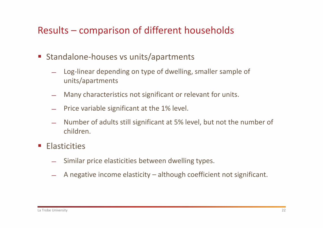
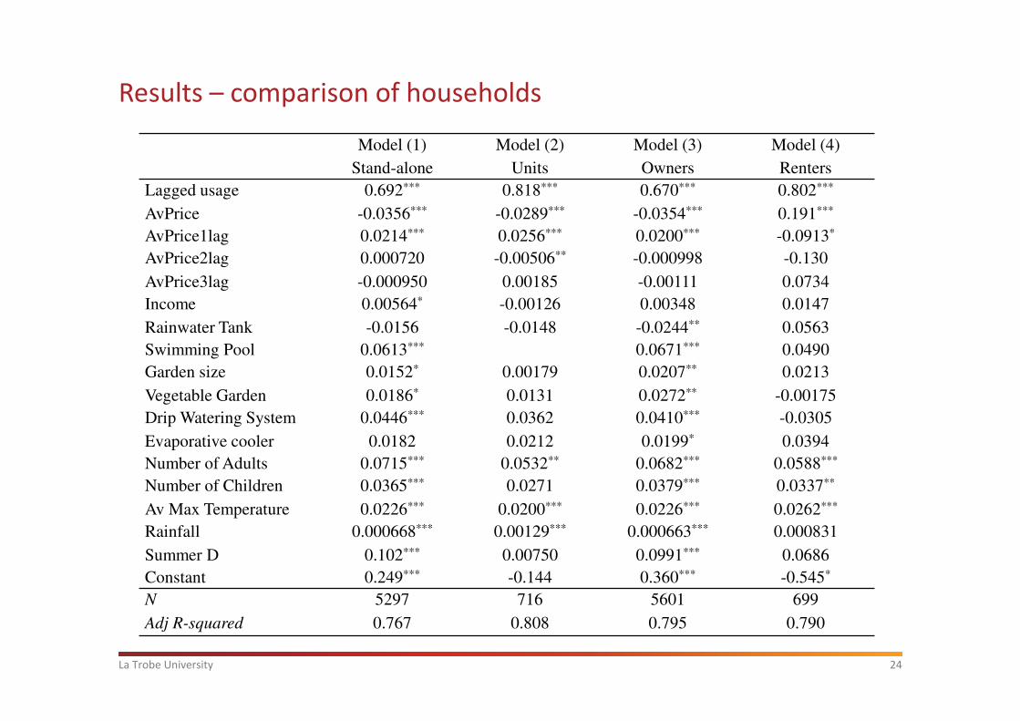
Results – comparison of different households
� Standalone-houses vs units/apartments
Log-linear depending on type of dwelling, smaller sample of
units/apartments
Many characteristics not significant or relevant for units.
Price variable significant at the 1% level.
Number of adults still significant at 5% level, but not the number of
children.
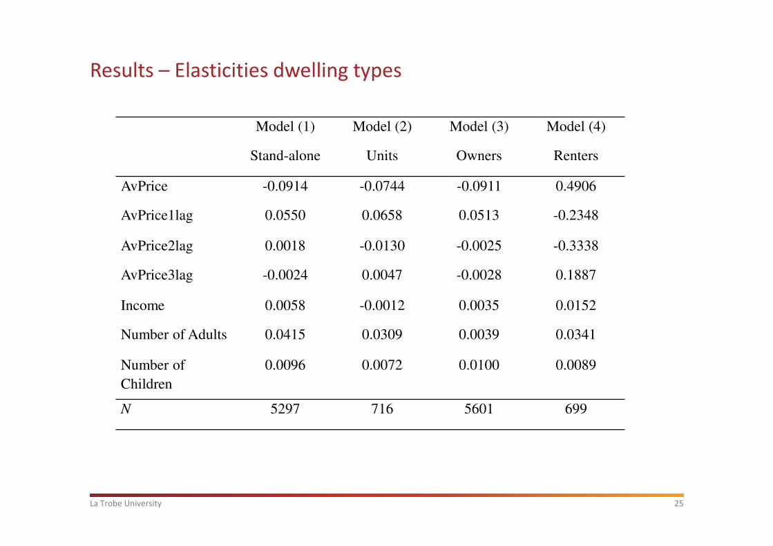
� Elasticities
Similar price elasticities between dwelling types.
A negative income elasticity – although coefficient not significant.

23La Trobe University
Results – comparison of different households
� Owners vs renters
Many of the dwelling characteristics not significant or relevant for
renters.
Price variable significant at the 1% level.
Summer dummy and rainfall not significant for renters.
� Elasticities
Price elasticity positive for renters – this reflects that the average price
does not include fixed costs. In this case the more usage the greater
the prices because of the increase block tariff.
Price elasticity for owners same as for stand-alone houses suggesting
the a 10% increase in price there is a 0.9% decrease in water usage.
24La Trobe University
Results – comparison of households
Model (1) Model (2) Model (3) Model (4)
Stand-alone Units Owners Renters
Lagged usage 0.692*** 0.818*** 0.670*** 0.802***
AvPrice -0.0356*** -0.0289*** -0.0354*** 0.191***
AvPrice1lag 0.0214*** 0.0256*** 0.0200*** -0.0913*
AvPrice2lag 0.000720 -0.00506** -0.000998 -0.130
AvPrice3lag -0.000950 0.00185 -0.00111 0.0734
Income 0.00564* -0.00126 0.00348 0.0147
Rainwater Tank -0.0156 -0.0148 -0.0244** 0.0563
Swimming Pool 0.0613*** 0.0671*** 0.0490
Garden size 0.0152* 0.00179 0.0207** 0.0213
Vegetable Garden 0.0186* 0.0131 0.0272** -0.00175
Drip Watering System 0.0446*** 0.0362 0.0410*** -0.0305
Evaporative cooler 0.0182 0.0212 0.0199* 0.0394
Number of Adults 0.0715*** 0.0532** 0.0682*** 0.0588***
Number of Children 0.0365*** 0.0271 0.0379*** 0.0337**
Av Max Temperature 0.0226*** 0.0200*** 0.0226*** 0.0262***
Rainfall 0.000668*** 0.00129*** 0.000663*** 0.000831
Summer D 0.102*** 0.00750 0.0991*** 0.0686
Constant 0.249*** -0.144 0.360*** -0.545*
N 5297 716 5601 699
Adj R-squared 0.767 0.808 0.795 0.790
25La Trobe University
Results – Elasticities dwelling types
Model (1) Model (2) Model (3) Model (4)
Stand-alone Units Owners Renters
AvPrice -0.0914 -0.0744 -0.0911 0.4906
AvPrice1lag 0.0550 0.0658 0.0513 -0.2348
AvPrice2lag 0.0018 -0.0130 -0.0025 -0.3338
AvPrice3lag -0.0024 0.0047 -0.0028 0.1887
Income 0.0058 -0.0012 0.0035 0.0152
Number of Adults 0.0415 0.0309 0.0039 0.0341
Number of
Children
0.0096 0.0072 0.0100 0.0089
N 5297 716 5601 699

26La Trobe University
Summary
� Demand is found to be inelastic
This is found using different estimators.
Across Dwelling types but not when accounting for renters (use
Marginal price)
� Other key determinants of water consumption:
Household characteristics such as garden size and swimming pool.
The size of the household.
Household income in the pooled OLS model is not significant.
Seasonal variation – as picked up by the summer variable.

27La Trobe University
Table 3 Summary statistics of variables
Variable Count Mean sd min max
Log Billed usage 11253 3.484603 .6999926 0 5.932245
Billed usage (Kl) 11440 40.13977 29.76123 0 377
Billed amount ($/quarter) 11440 250.6856 156.3248 -2033.06 1741.35
Total cost ($/quarter) 11440 281.3342 145.3623 0 2107.392
Marginal Price ($/Kl) 11253 1.428 .8818219 .3037 2.597
Average Price ($/Kl) 11253 8.962852 8.00437 2.859612 157.5075
Income 8560 3.596262 1.7428 1 7
Rainwater Tank 10704 1.31988 .4664518 1 2
Swimming Pool 10704 1.091181 .2878796 1 2
Garden size 10704 1.898356 .7203228 1 3
Vegetable Garden 10704 1.41704 .4930927 1 2
Drip Water System 10704 1.252616 .4345328 1 2
Evaporative cooler 11344 1.335684 .4722499 1 2
Number of Adults 11440 2.025175 .796484 0 8
Number of Children 11440 .9272727 1.175689 0 6
Average Max Temp (°C) 11440 21.055 4.651484 15.43 28.73
Rainfall (ml) 11440 160.175 61.34025 54.8 344.2

Thank you
latrobe.edu.au CRICOS Provider 00115M