Embed Size (px)
Citation preview

Chapter 12
A P P R O X I M A T I O N , P E R T U R B A T I O N , A N D P R O J E C T I O N
M E T H O D S IN E C O N O M I C A N A L Y S I S
KENNETH L. JUDD*
Hoover Institution, Stanford University and National Bureau of Economic Research
Contents
1. Introduction 2. The uses of approximation ideas: An overview 3. The mathematical foundations of regular perturbation methods
3.1. The meaning of "approximation"
3.2. Taylor series approximation
3.3. Rational approximation
3.4. hnplicit function theorem
3.5. Generalizations to function spaces
4. Applications of regular perturbation methods to economics 4.1. Comparative statics: A simple rule of thumb in tax theory
4.2. Comparative dynanaics: A canonical problem
4.3. Perturbing dynamic equilibria
4.4. The stable manifold theorem and applications to economic theory
4.5. Pel~turbing functional equations from recursive equilibrium analyses
5. Bifurcation methods 5.1. Applications of the Hopf bifurcation to dynamic economic theory
5.2. Gauge functions
5.3. Bifurcation applications to stochastic modelling
6. Asymptotic expansions of integrals 6.1. Econometric applications of asymptotic methods
6.2. Theoretical applications of Laplace's method
511 513 515 515 516 516 517 517 519 520 520 521 524 527 54O 541 542 542 545 547 547
* This research was supported by NSF Grant SBR-9309613. The author gratefully acknowledges commeuts from Bo Li, Ariel Pakes, John Rust, and Ben Wang.
Handbook of Computational Economics, Volume I, Edited by H.M. Amman, D.A. Kendrick and J. Rust ~) 1996 Elsevier Science B.!~ All rights reserved.
510 K.L. dudd
7. The mathematics of L p approximations 7.1. Orthogonal polynomials 7.2. Least-squares orthogonal polynomial approximation 7.3. Interpolation 7.4. Approximation through interpolation 7.5. Approximation through regression 7.6. Piecewise polynomial interpolation 7.7. Shape-preserving interpolation 7.8. Multidimensional approximation
8. Applicat ions of approximation to dynamic programming 8.1. Discretization methods 8.2. Multilinear approximation 8.3. Polynomial approximations
9. Projection methods 9.1. General projection algorithm
10. Applicat ions of projection methods to rational expectations models 10.1. Discrete-time deterministic optimal growth 10.2. Stochastic optimal growth 10.3. Problems with inequality constraints 10.4. Dynamic games 10.5. Continuous time problems 10.6. Models with asymmetric information 10.7. Convergence properties and accuracy of projection methods
11. Hybr id perturbat ion-project ion method 12. Conclusions References
548 548 549 551 552 554 554 556 557 560 562 563 563 563 565 569 569 572 574 574 575 575 577 578 58O 581

Ch. 12: Approximation, Perturbation, and Projection Methods in Economic Analysis 511
This article examines local and global approximation methods which have been used or have potential future value in economic and econometric analysis. While these methods are familiar, they are seldom developed within a general, formal analytical framework, a fact which has hindered understanding of these techniques and limited their application. We attempt to review and unify this literature, showing connections which have been ignored, and pointing out potential new directions. We first re- view the foundations of basic asymptotic, or, perturbation, methods, and discuss their applications to economic modelling and econometrics. We next discuss global ap- proximation methods, including orthogonal polynomials, interpolation theory, shape- preserving splines, and neural networks. We present the related projection method for solving operator equations, and illustrate its application to dynamic economic analysis, dynamic games, and asset market equilibrium with asymmetric information. Finally, we discuss how the hybrid perturbation-projection method combines the complemen- tary strengths of local approximation procedures and the projection method to produce a promising new method.
1. Introduction
The key technical problem in much of economic analysis is the determination of some unknown function. Important examples include the optimal policy functions of economic agents (such as the consumption function in macroeconomics), equilibrium price functions dynamic models, equilibrium strategies in games, and inference rules and price functions in asymmetric information problems. The usual approach is to make functional form assumptions on the structural elements of a model which lead to closed-form solutions for these functions; prominent examples of this approach are the linear-quadratic competitive structures discussed in Hansen and Sargent [60], the linear-quadratic dynamic game structure exposited in Kydland [82, 83], the linear risk tolerance and Gaussian returns assumptions in Merton [96], and the exponential- Gaussian structure in Grossman [54]. Unfortunately, the desire for a closed-form solution often restricts the analysis. While these special cases may suffice for some purposes, they are often inadequate for a robust analysis. Such robustness is important for both theoretical analysis, where important elements may be ignored in cases with closed-form solutions, and in empirical work where misspecification of tastes and technology can ruin an otherwise valid approach.
The alternative is to assume more general and flexible functional forms and use approximation ideas to compute functions which are "close" to the true solution. In the first section we remind the reader of a variety of theoretical and empirical prob- lems for which these methods are useful. In the rest of the paper, we will review the two basic approaches to the approximation of functions and the approximate so-. lution of operator equations, representing two different kinds of data and objectives, and introduce a third which combines the strengths of the first two methods. Loca l

512 K.L. Judd
approximations take as data the value of the unknown function f and its derivatives at a point x0 and constructs a function which matches those properties at x0. These constructions rely on Taylor's theorem, the implicit function theorem, and bifurcation theory, and lead to the construction of Taylor or Pad6 series, or other approximations of a simple form. These methods are called perturbation, or asymptotic, methods. The basic idea of asymptotic methods is to formulate a general problem, find a particular case which has a known solution, and then use that particular case and its solution as a starting point for computing approximate solutions to "nearby" problems. These methods are widely used in mathematical physics, particularly in quantum mechanics and general relativity theory, with much success. While economists have often used special versions of perturbation and asymptotic techniques, such as linearizing around a steady state, they often provide little formal justifications for their procedures, and sometimes proceed in ad hoc and potentially invalid fashions. This has lead to some coniusion as to the differences among various procedures. This is plausibly one rea- son why economists have generally not exploited the full range and power of these approximation techniques.
We will give simple examples of the perturbation methods and indicate the more substantive uses which have appeared in the economics literature. These applications include theoretical analyses of sunspot equilibria as well as quantitative analyses of economic policies and business cycles. We will interpret the phrase "computational economics" broadly in this chapter. The perturbation analyses which theorists have done has been viewed as pure theory, and the authors made no apparent use of a com- puter. However, much of this work is really the outcome of algebraic manipulations which could be automated by symbolic mathematics software, such as Mathematica, Maple, or Macsyma. We take the view that in the future such theoretical analyses will be done by computer software, and is an interesting new avenue for computational economics. This literature is included here also because the linear approximations which these authors compute do have value as numerical approximations, and it is instructive to compare these methods with other "linear approximation" methods used in economics. Furthermore, these linear approximations are just the first step in higher-order Taylor series expansions which themselves may have substantial numer- ical value, even though this fact is generally not utilized in either the theoretical or applied literatures.
The other approaches to approximation are more global in nature. L p approximation
takes a given function f and finds a "nice" function 9 which is "close to" f in the sense of some L p norm. To compute an L p approximation of f , one ideally needs the entire function, whereas we generally have information about f at only a finite number of values. Interpolation is any procedure which finds a "nice" function which exactly fits a finite set of prescribed conditions. Regression is similar to L p
approximation in that a some L p norm is minimized, an L 2 norm in the case of least squares and L ~ in the case of minimum absolute deviation. Regression also lies between L p approximation and interpolation in that it uses n points of data to
Ch. 12: Approximation, Perturbation, and Projection Methods in Economic Analysis 513
produce an approximation with m < n free parameters which "nearly" satisfies the data. These approximation methods form the basis for projection methods, also known as weighted residual methods, for solving functional equations. Projection methods have been increasingly used in the physical sciences over the past twenty years. They have been used to solve various economic problems, ranging from dynamic growth models, dynamic games, and asset market equilibria with incomplete information.
Both perturbation and L p approximation methods are important because of the in- creasing role of computation in economic analysis. Many computational economists eschew sophisticated approximation techniques, believing that simple methods of ap- proximation combined with supercomputer technology will solve any problem they might have. This is not the attitude taken in other computationally intensive fields. In fact, an examination of the numerical analysis literature shows that over the past fifty years advances in numerical analysis have improved algorithm speed as much as hardware advances. Rice [108] presents a formal and substantive discussion of this issue for the problem of solving two- and three-dimensional elliptic partial differen- tial equations, a class of numerical problems which arise naturally in continuous-time stochastic economic modelling. He argues that we were able to solve these problems 4 million to 50 billion times faster in 1978 than in 1945, of which a factor of 2,000 to 25 million can be attributed to software improvements, and a factor of 2,000 to hardware improvements. One reason for this improvement has been the application of the basic approximation ideas we present below. It is clear from examination of the mathematical and economic literature that even a modest application of modern approximation techniques can substantially improve the efficiency of most computa- tional methods in economics. The objective of this review is to be retrospective and review actual applications, but also to be prospective and indicate where a more in- tensive use of well-known mathematical techniques can expand the range and quality of these applications in economics.
After discussing perturbation and projection methods, we move to a third approach to approximation which combines perturbation and projection methods. The perturba- tion and projection methods of solution differ substantially in their focus and proce- dures. However, we shall see that their strengths and weaknesses are complementary. This complementarity implies that a combined analysis using both methods will al- low economists to analyze many economic problems in a robust and reliable fashion. This combined method is called the hybrid perturbation-Galerkin procedure. We will illustrate its advantages and potential in a simple example.
2. The uses of approximation ideas: An overview
Economic modelling problems have used a variety of approximation methods. In dy- namic programming problems, one wants to solve out for the value function and the corresponding policy rule, which in turn are needed for an empirical analysis of the

514 K.L. Judd
data. The closed-form approach l to this problem is exemplified in Sargent's [116] analysis of dynamic labor demand. However, the linear-quadratic approach has limi- tations. Rust [111] exemplifies the alternative approach where one assumes arbitrary tastes and technology and approximately solves the dynamic programming problem of the agents and for likelihood models for the data. However, Rust uses the very conservative discrete-state approximation method which is reliable but slow. The ap- proximation ideas we discuss below have been successful in solving many dynamic programming problems which are more general than the linear-quadratic case but with substantially greater efficiency than the discrete-space approximation method. These solutions could also be used in maximum likelihood econometric procedures where such an increase in speed would be important.
The approximation ideas we discuss below have also been used in rational expec- tations equilibrium analysis. Closed-form solutions are rare; agricultural economists realized the futility of this back in 1958 with Gustafson's [56] work on grain stock- piling. A critical aspect of that problem is the nonnegativity constraint on grain stock- piles. This constraint leads to kinks in the storage rules and price functions. Gustafson used piecewise linear functions to approximate the relation between current price and the current total grain stock. Williams and Wright [123-125] extended the Gustafson analysis to include elastic supply. An important innovation in their solution was their observation that the conditional expectation of the future grain price is a smooth func- tion of the current state of the market, and that this conditional expectation function characterizes equilibrium. This observation suggests that equilibrium can be approxi- mated by low-order polynomial approximation of the conditional expectation function which characterizes equilibrium. This leads to a considerable improvement in effi- ciency over the alternative of using discrete-state or piecewise linear approximations of the current price law. Helmburger and Miranda [98] also use this approximation idea to solve equilibrium. More recently, Christiano and Fisher [32] use the same idea to model general equilibrium where a nonnegativity constraint on gross investment will occasionally bind.
These approximation methods are also important in empirical work on structural models of commodity markets. Deaton and Laroque [43] used approximations of the rational expectations equilibrium to compute methods of moments estimates in a fully structural model of several commodity markets,
Dynamic games also have a similar dichotomy. Kydland exemplifies the closed- form approach to linear-quadratic games, whereas Kotlikoff, Shoven, and Spivak [80]
l Some may argue that the linear-quadratic model typically does not have a closed-form solution because it is generally necessary to solve a Riccati equation, or, as in the case of dynamic games, a coupled system of Riccati equations. While there are nontrivial problems associated with solving Riccati equations, we currently have methods which are so reliable and accurate that the solutions are treated as if they were closed-form solutions with no computational error. Since the approximation problems are much worse when we leave the linear-quadratic paradigm, linear-quadratic modelling is, for the purposes of this review, more like closed-form modelling than the approximate solutions we will discuss.

Ch. 12: Approximation, Perturbation, and Projection Methods in Economic Analysis 515
take a smooth approximation approach to solving a more general dynamic game. Judd [71] and Miranda and Rui [99] use modern approximation theory to solve non- linear dynamic games.
The most common use of perturbation methods is the method of "linearizing around a steady state". Such linearizations tell us how a dynamical system evolves near a steady state, and we can also use them to compute how a system reacts to shocks which move the steady state, such as tax policy or monetary policy changes. A particularly important case of this was Magill [93], who suggested that the linear approximations of stochastic growth models be used in macroeconometric analysis. Kydland and Prescott [85], and many later macroeconomists have successfully used a linear approximation computational approach to examine the empirical strength of the Real Business Cycle hypothesis. Similarly, many authors used linearization methods to analyze the impact of macroeconomic policy on dynamic equilibrium.
The key fact is that perturbation methods are just ways to take derivatives in com- plex problems. This implies that they have a variety of uses. For example, in maximum likelihood estimation, one must repeatedly compute derivatives of the likelihood func- tion. Zadrozny [127] discusses how to compute such derivatives analytically in the case of linear quadratic models. For more general models, computing such derivatives is generally done numerically. However, perturbation methods could be used to solve for these derivatives analytically with considerable gains in accuracy and speed.
These are just a few examples of how approximation ideas are important in com- putational aspects of both theory and econometrics. We shall now discuss the formal mathematics behind these approximation ideas and illustrate their applications in sim- ple examples.
3. The mathematical foundations of regular perturbation methods
The most basic local approximation techniques are called regular perturbation meth- ods. They are based on a few basic theorems including the well-known Taylor's theorem and the implicit function theorem for/~n as well as extensions to operators on infinite-dimensional spaces. We will first state the basic theorems which provide the foundation for regular perturbation methods in this section, and give examples of their use in the next section.
3.1. The meaning of "approximation"
We often use the phrase " f (x ) approximates 9(z) for z near z0", but the meaning of this phrase is seldom made clear. One trivial sense of the term is that f(zo) =- 9(zo). While this is certainly a necessary condition, it is generally too weak to be a useful concept. Approximation usually means at least that f~(zo) = 91(zo) as well. In this
516 K.L. Judd
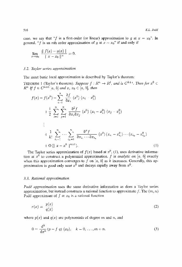
case, we say that " f is a first-order (or linear) approximation to 9 at x = x0". In general, " f is an nth order approximation of 9 at x = xo" if and only if
lim I] f ( x ) - g ( x ) = O. ~ " I l x - x o [ I n
3.2. Taylor series approximation
The most basic local approximation is described by Taylor's theorem:
THEOREM 1 (Taylor's theorem). Suppose f • R n --+ R 1, and is C k+l. Then for x ° c R n I f f E C n+l [a, b] and x, xo E [a, b], then
f ( x ) = f ( x °) + ~x~ (x°) (x~ - x °) i=l
1 ov
M7 ~,, " ' " ~ X i l , , . ~ X i k (X0)(X~I--xOi)' ' '(Xik--,~7Ok) i1=I ik=l
+ O (ll x - x ° Ilk+l). (1)
The Taylor series approximation of f ( x ) based at x °, (1), uses derivative informa- tion at x ° to construct a polynomial approximation, f is analytic on [a, b] exactly when this approximation converges to f on [a, b] as k increases. Generally, this ap- proximation is good only near x ° and decays rapidly away from x °.
3.3. Rational approximation
Padd approximation uses the same derivative information as does a Taylor series approximation, but instead constructs a rational function to approximate f . The (m, n) Pad6 approximant of f at x0 is a rational function
r ( x ) - p(x) (2) q(x)
where p(x) and q(x) are polynomials of degree m and n, and
d k 0 = - d - x ~ ( p - f q ) (x0), k = 0 , . . . , m + n . (3)
Ch. 12: Approximation, Perturbation, and Projection Methods in Economic Analysis 517
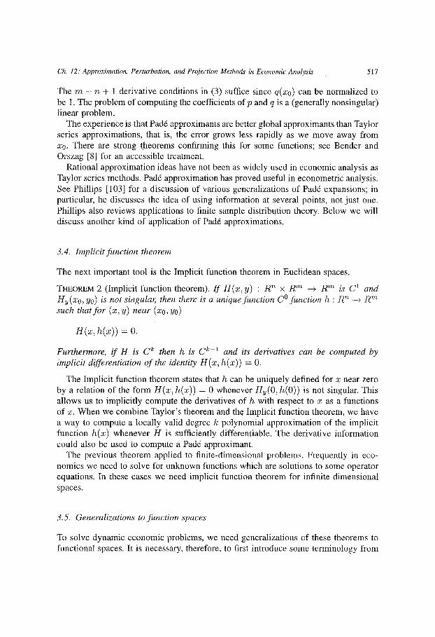
The m + n + 1 derivative conditions in (3) suffice since q(xo) can be normalized to be I. The problem of computing the coefficients of p and q is a (generally nonsingular) linear problem,
The experience is that Pad6 approximants are better global approximants than Taylor series approximations, that is, the error grows less rapidly as we move away from x0. There are strong theorems confirming this for some functions; see Bender and Orszag [8] for an accessible treatment.
Rational approximation ideas have not been as widely used in economic analysis as Taylor series methods. Pad6 approximation has proved useful in econometric analysis. See Phillips [103] for a discussion of various generalizations of Pad6 expansions; in particular, he discusses the idea of using information at several points, not just one. Phillips also reviews applications to finite sample distribution theory. Below we will discuss another kind of application of Pad6 approximations.
3.4. Implicit function theorem
The next important tool is the Implicit function theorem in Euclidean spaces.
THEOREM 2 (Implicit function theorem). I f H ( x , y) : R ';~ x R "~ --+ R "~ is C j and Hv(xo, fro) is not singular, then there is a unique function C° function h : R n -+ R m such that for (x, y) near (xo, Yo)
H(x, h(x)) = o.
Furthermore, i f H is C k then h is C k - j and its derivatives can be computed by implicit differentiation o f the identity H ( x , h(x) ) -~ O.
The Implicit function theorcm states that h can be uniquely defined for x near zero by a relation of the form H ( x , h(x)) = 0 whenever Hy(0, h(0)) is not singular. This allows us to implicitly compute the derivatives of h with respect to x as a functions of x. When we combine Taylor's theorem and the Implicit function theorem, we have a way to compute a locally valid degree k polynomial approximation of the implicit function h(x) whenever H is sufficiently differentiable. The derivative information could also be used to compute a Pad6 approximant.
The previous theorem applied to finite-dimensional problems. Frequently in eco- nomics we need to solve for unknown functions which are solutions to some operator equations. In these cases we need implicit function theorem for infinite dimensional spaces.
3.5. Generalizations to function spaces
To solve dynamic economic problems, we need generalizations of these theorems to functional spaces. It is necessary, therefore, to first introduce some terminology from

5 l 8 K.L. Judd
functional analysis, and state a generalization of the implicit function theorem which has a straightforward computational implementation.
Suppose that X and Y are Banach spaces, i.e., normed complete vector spaces. A map M : X k -+ Y is k-linear if it is linear in each of its k arguments. It is a power map if it is symmetric and k-linear, in which case it is denoted by M:C k = M ( x , x , . . . , x). The norm of M is constructed from the norms on X and Y, and is defined by
IIMII : sup IIM(xl , :C2, . . . , xk)ll. I I : ~ d l = l , i = 1 , 2 . . . . . k
For any fixed :Co in X , consider the infinite sum in Y
O<3
Tx : Z -
k = l
(4)
where each of the Mk is a k-linear power map from X to Y. When the infinite series in (4) converges, T is a map from X to Y. The majorant series for T is
IIMk[I - x01l k. k = 0
The important fact is that T will converge whenever its majorant series does.
DEFINITION 3. r is analytic at xo if and only if, for some neighborhood of x0, it is defined and its majorant series converges.
With these definitions, we can now state an analytic operator version of the Implicit Function Theorem, taken from Zeidler [128].
THEOREM 4 (Implicit function theorem for analytic operators). Suppose that
O4)
= "M,j
n,k=O
(5)
defines an analytic operator, F : U C R × X -+ Y, where U is a neighborhood o f (0, O) in R × X . Furthermore, assume that F(0, 0) = 0 and that the operator Mol : X --+ Y, representing the Frechet cross-partial derivative at (0, 0), is invertible. Consider the equation
F(e , x(e)) = 0 (6)
implicitly defining a function x(e) : R --~ X . The following are true:
1. There is a neighborhood of 0 E R, V, and a positive number, r > O, such that (6) has a unique solution x(e) with [Ix(c)ll < r for each e E V.

Ch. 12: Approximation, Perturbation, and Projection Methods in Economic Analysis 519
2. The solution, x(e), of(6) is analytic at e = O, and, ]or some sequence of x~ in X , can be expressed as
oo : n (7)
where the coefficients xn can be determined by substituting (7) into (6) and equating coefficients of like powers of e.
3. The radius of convergence of the power series representation in (7) is no less than that o f the analytic map, z(e) : R --+ R, defined implicitly for some neighborhood of O by
o o
o : Z IIMnkll <8) n , k = O
Furthermore, fbr some sequence Zn of real numbers,
o o
n=O
represents the solution to (8) and IZnl > [IX,~ll.
See Zeidler [128] for a proof and discussion of this implicit function theorem. The mathematics of applying this method turns out to be elementary since the task is reduced to recursive computation of xn terms, in term-by-term approach described above. The only requirement is to set up the problem so that it is expressed as an analytic operator with a nondegenerate radius of convergence. This theorem shows that the logic and intuition from the finite-dimensional implicit function theorem generalizes naturally and straightforwardly for analytic operators.
4. Applications of regular perturbation methods to economics
There have been many uses of local approximations in economics, implicit and ex- plicit. The topic of comparative statics is nothing more than applications of the implicit function theorem. Comparative dynamics are technically more difficult problems, but fit into the same general framework. Recognizing these similarities will help us solve difficult problems. We will review some basic applications which have appeared and give examples of some possible future uses.
520 ICL Judd
4.1. Comparative statics: A simple rule of thumb in tax theory
Comparative statics are just basic applications of the implicit function theorem. One simple example of applying perturbation ideas is the impact of a tax on equilibrium. Suppose that D(p) is demand at consumer price p, that S(p) is supply at producer price p, and that a per unit tax of r is applied. Then the equilibrium consumer price at tax rate ~- can be expressed as the function p( r ) which is implicitly defined by D(p(r) ) = S(p(r) - r). We can expand this relation around r = 0, the tax-free equilibrium case, to study the impact of the tax on equilibrium. This analysis leads, for example, to the useful rule of thumb that the efficiency cost of a tax equals l(r/D + r /s)r 2 where rlD and Us are the demand and supply elasticities at the r = 0 case. This quadratic approximation has been used extensively to intuitively discuss tax policies and as the formal basis for some quantitative tax analysis, as in the Barro [5] analysis of optimal tax policy.
This tax example is just one simple case where simple perturbation formulas, more commonly described as comparative statics, are useful approximations. We next ex- amine dynamic applications of these perturbation ideas.
4.2. Comparative dynamics: A canonical problem
Since it will be frequently used below, we will now describe a simple continuous- time 2 model of economic growth. Let k be the capital stock, e the rate of consumption, and f ( k ) the rate of output. Assume that the intertemporal utility function of the representative agent is f ~ e-ptu(c(t)) dr, and that the capital stock evolves according
to k, = f ( k ) - e. The corresponding optimal growth problem is
V(ko) ~ max foo e -pt u(c) dt, ~(t) Jo
= f ( k ) - c (9)
k(0)- k0
where V(k) is the value function. Our examples will study the solution to this op- timal growth problem. We will also examine the representative agent version of this problem. The competitive equilibrium will correspond to the social planning prob- lem in the perfectly competitive, distortion free case, but not otherwise. We will also examine the equilibrium problem when taxes are present. While this model and its stochastic generalization appears to be special, it is in the same general family of dynamic optimization problems investigated by the papers of Sargent and Rust.
2It will be obvious that all of these methods can be applied in the same way to discrete-time models. Since there is no substantive distinction between the discrete-time and continuous-time literatures, I will discuss continuous-time and discrete-time papers together.
Ch, 12: Approximation, Perturbation, and Projection Methods in Economic Analysis 521
4.3. Perturbing dynamic equilibria
To illustrate the essential features of perturbation methods applied to dynamic equi- libria, we apply them to study the effects of policy changes in a dynamic model of equilibrium with taxation. Brock and Turnovsky [21] shows that if we take the simple growth model behind (9) and add a tax on capital income, the resulting equilibrium solves the system of differential equations
~=3'(c) c (p - f ' ( k ) (1 - r ) ) ,
k = f ( k ) - e - g (10)
where 3@) ~ u'(c)/(cu"(c)) is the rate of intertemporal substitution in consumption, r(t) is the tax on capital income at time t, 9(t) is government expenditure (on goods which do not affect utility) at t. The tax rates are exogenous, and c and k are the unknowns to be determined. Note that this includes the special case of r = g = 0, which characterizes (9). The boundary conditions for (10) are the initial condition on the capital stock
k(O) = too (11)
and a stability condition on consumption
0 < lim c(t) < o c . t--+oo
(12)
The conceptual experiment is as follows. We assume that the "old" tax policy was constant, r ( t ) = f , and that it has been in place so long that, at t = 0, the economy is at the steady state corresponding to ¢. Note that this also assumes that for t < 0, agents assumed that r ( t ) = ? for all t, even t > 0. Hence, at t = 0, k(0) = k *s. Suppose, however, that at t = 0, agents are told that future tax policy will be different. Say that they find out that the new tax rates are ? + r ( t ) , t /> 0, that is r ( t ) will be the change in the tax rate at time t. Similarly, they are told that the new expenditure policy is ~0 + 9(@ We also allow the possibility that the capital stock at t = 0 is changed by n. The new system is
d=7(c)c(p - ft(h)(¢ + -r(t))),
]c=f(k) - c - (~ + 9(t)) (13)
together with k(0) = k s* + ~, and (12). We will use perturbation methods to approx- imate the effects of the new policies r and g on the dynamic paths for k and c.

522 K.L. Judd
We need to parameterize the new policy so that it fits the perturbation approach; that is, we need to imbed the shocked system (13) in a parameterized collection set of problems of the form F(c , k, t, e) = 0. We do this by defining
~(t, ~) = e + ~ ( t ) , g( t , ~) = o + ~9(t), k(o, ~) = k ss + ~
and the corresponding continuum of BVP's
ct(t, e) = 7(c(t , e)) c(t, e) (p - f ' ( k ( t , e))(1 - T(t, e))),
kt( t , e) = f ( k ( t , e)) - c(t, e) - g(t, e), (14)
k (0, e) = k ss + e~
plus (12). The system (14) implicitly defines consumption and capital paths for any value of
e. In that way, it fits into our general implicit function framework in that we have an expression F(c , k, t, c) = 0 which implicitly defines the paths c(t) and k(t) . As long as the functions involved in (14) are locally analytic, we can apply Theorem 4 above. With this apparatus in hand, we can now solve for the first-order perturbation of (14).
To solve for first-order approximations of the impact of e on c and k, we differentiate (14) with respect to e, evaluate the resulting differential equation at e = 0, and arrive at the following linear differential equation system for the unknown functions c~ (t, 0) and k~ (t, 0):
c~t(t,O) = 7 ( c s~) c s~ ( - f" (kSS)(1 - f ) k e ( t , O ) + ( p - f t (k~S)( -~-~( t ,O)) ) ) ,
k~,(t, o) = f ' (k~ ' )k~( t , O) - c~( t , O) - g ( t ) , (15 )
k~ (0, O) =
plus the condition that c~ and k~ are both bounded. This is a linear boundary value problem with constant coefficients, which can be solved analytically. This is typical of perturbation methods: differentiate a nonlinear problem and one will arrive at a linear problem of the same type.
We then solve for c~(t, 0) and k~(t, 0) from (15). The result will allow us to compute a linear approximation for c(t, 1) and k(t , 1), the consumption and capital paths under the tax and spending changes; they are
c(t, 1) ~ f ( k ~ ) - ~ + c~(t, 0),
k( t , 1) ~ k ss + k~(t, 0).
One can also compute the derivative of any dynamic quantity, such as lifetime utility and tax revenue, with respect to e, thereby computing the marginal change in the consumption and capital path per dollar of extra revenue, per util of extra utility, or relative to any other quantity.

Ch. 12: Approximation, Perturbation, and Projection Methods" in Economic Analysis 523
The resulting solutions can be very informative. For example, the initial shock to net investment (denoted by the derivative of I - f (k) - e with respect to e at t = 0) is
I~(O)- 7cP T(p)+(f'(k s~)-p)ec÷pG(~)-g(O) (16)
where
# -- I 2(1 - ?) 1 + 1 + crOK
is the positive eigenvalue of the linearized system (15), OK is capital's share of income, Or is labor's share, and 0c is the steady state share of output which goes to consumption. G(s ) and T ( s ) are the Laplace transforms 3 of the policy perturbations 9( t ) and ~-(t).
Perturbation methods yield algebraic formulas for quantities of interest. For exam- ple, the formula (16) tells us many things. First, future tax increases reduce investment. However, their effect is proportional to T(#) , which is essentially the average tax in- crease discounted at the positive eigenvalue, #. From (17) it is clear that # exceeds i f ( k ) , the marginal product of capital and p, the after-tax return. Hence, future tax increases are heavily discounted when determining their impact on current investment. Second, government spending has an ambiguous impact on investment - current gov- ernment spending depresses investment and future spending increases investment, but again the future impact is discounted at rate #. Third, since investment and output are related, we also know the initial impact of this policy shock on output. For ex- ample, if a future tax increase causes current investment to fall, then output in the future will also fall. Note that these shocks could be nonconstant, allowing us to consider partially anticipated shocks. These simple calculations address basic issues in macroeconomics.
Fourth, the presence of t~ in (14) allows us to use the same approach to compute the effect of changes in the initial capital stock on consumption. The effect is intuitive: an increase in the capital stock of ~ will increase output by ~ f ' ( h ss) = ~p / (1 - "~) but will increase consumption by #t~, but # > f ' ( k ss) implies that the increase in con- sumption is greater. Therefore, this procedure also tells us that the slope of the equi- librium policy function for consumption is #.
We can also use this method to approximate solutions to the optimal growth model. We chose the tax example to make clear that the presence of a social planning equiv- alent plays no role in this procedure. However, if taxes and government spending are
3If f( t) : R 1 -~ R n, then the Laplace transform of f( t) is L ( f } : R l -+ R n, where L(f}(s) O o
f , e-~t f ( t ) dt.
524 K.L. Judd
zero, then the problem reduces to the social planner 's optimal growth problem. For example, the presence of the parameter ~ in (14) means that the linear approximation to the consumption policy function near the steady state is F~-
4.4. The stable manifold theorem and applications to economic theory
The analysis above is just a simple example of what perturbation analysis can do. Extending this type of analysis to several states is important in economics. These additional states will arise when we include heterogeneous capital or heterogeneous agents to our model. In this section we review the stable manifold theorem, 4 which is the general statement of the linear approximation theory in dynamical systems, and its applications to economics. However, we will also note that we can compute approximations which go beyond those derived from the stable manifold theorem.
4.4.1. Multidimensional dynamics
The methods used above can be extended to the case of several state variables by applying basic linear algebra and differential equation theory. The most used math- ematical theorem in this regard is the stable manifold theorem. Suppose we have a dynamic system
2 = g(z) (18)
with a stationary point at Z*; that is, 9(Z*) = 0. Then the local behavior of (18) for Z near Z* is linearly approximated by the linear system
= A z (19)
where A = 9z(Z*) and z -= Z - Z*. The solution to (19) is z(t) = e At zo .5 The stable manifold theorem essentially says that the local behavior of (18) near Z* is approximated with first-order accuracy by the local behavior of (19). In particular, if the linear system (19) has a k-dimensional stable space near Z*, then (18) has a k-dimensional stable manifold 6 near Z*.
This is a common situation in dynamic growth models, with and without distortions. Let Z = (X, Y) where X is a list of predetermined variables and Y is a list of free variables; we use here the terminology of linear rational expectations models, as in
4We shall just discuss the procedure which is .justified by the stable mmlifold theorem. An interested reader can find a formal statement of the stable manifold theorem in Coddington and Levinson [35].
SFor discrete time systems, Zt+l = 9(Zt), Z* = 9(Z*), zt+l = Azt, and zt = Atzo. 6A stable manifold is a manifold, M, such that if z(to) is in M than Z(t) is in M for t >tl l and
converges to Z*.
Ch. 12: Approximation, Perturbation, and Projection Methods in Economic Analysis 525
Blanchard and Kahn [12], for example. The predetermined variables are the state variables, such the distribution of the capital stock across sectors, or the distribution of wealth. The free variables are the decision variables, such as consumption and labor supply, and prices, all of which are endogenous at each moment. Suppose that there is a stationary point at Z* = (X*, Y*). Then the local behavior of the system is linearly approximated by (19)and the solution is z(t) = e At (xo, Yo), where x - X - X*, y - Y - Y*, and y0 is chosen to keep z(t) bounded asymptotically. Let 3;(x0) be the set of all possible values for the free variables which together with the predetermined variables being equal to x0 will imply a bounded path for z(t). 3;(xo) may be a single value or a set of values.
In many economic models, Y(x0) is a single-valued function which generates much valuable information, such as the dependence of prices, output, labor supply, and consumption on the state variables. As in the one-dimensional case, in general, they will allow one to compute linear approximations to the multidimensional equilibrium decision rules, even when the equilibrium cannot be reduced to a social planning problem. This procedure (which is equally valid for continuous-time and discrete- time systems) for computing a linear approximation is well-known; it is presented, for example, in detail in Chapter 6 of Stokey and Lucas [119]. Anderson [2] presents computer programs in Mathematica for solving such problems in discrete-time.
4.4.2. Comparative dynamics
The general theory of such perturbations for optimal control problems has been worked out in a variety of papers. Oniki [101] and Araujo and Scheinkman [3] proved that optimal paths were differentiable with respect to parameters. Treadway [121] and Mortenson [100] used a heuristic approach to derive explicit formulas for local ap- proximations near steady states. Lucas [92] and Otani [102] provided approximation formulas and formal justifications for them, the latter for the general optimal control problem. Caputo [25, 24] derived Slutsky - like expressions for comparative dynam- ics problems, and Lafrance and Barney [86] extended the analysis to the case of nondifferentiable constraints.
While the tax example in (15) above was quite simple, the robustness of the method to dynamic equilibrium analysis is obvious. This approach has been used to analyze many questions in dynamic economic policy. One can add labor supply, and other tax instruments. Judd [66, 68, 67] used this method to calculate the marginal effi~ ciency cost of various tax innovations, and related impulse responses to tax changes for several macroeconomic variables. Laitner [87-89, 91] has written a series of pa- pers on comparative dynamics, and applying them to difficult problems in dynamic tax incidence. His work includes Overlapping generations applications of perturba- tion methods and large-dimension applications of the linearization procedure. Bovem berg [t6, 18, 17] has used these methods to analyze international economic questions.
526 K.L. Judd
He has computed the impact of taxation on capital flows, trade patterns, and terms of trade in dynamic models of international trade. All of these authors 7 use lineariza- tions around the steady state to compute quantitative estimates of the impact of policy shocks. It is clear that these procedures can be used to analyze models with imperfect competition and externalities as well.
The linearization procedures appear to be much faster than alternative numerical methods, such as shooting. The disadvantage is that linearization procedures can produce only the first-order effects, and may miss higher-order effects. We next turn to that issue.
4.4.3. Higher-order approximations
The stable manifold theorem calculation yields just linear approximations. However, proceeding as we did above, one could also compute second order approximations. This is typically not done, but there is no theoretical difficulty. In fact, when we compute the second differential of (14) one finds that the differential equations for c~(t) and k~(t) are the same as the differential equations for c~(t) and k~(t) in (15) except for different forcing terms. More specifically, if we write (15) in the form gc = Ax + ~(t), where x = (c~, k~), then the corresponding equation for e~(t) and k,~(t) has the same form except for the ~p(t) term. Since the difficult part of solving any linear differential equation lies in dealing with the linear operator A, we see that solving for c,,(t) and k,,(t) is essentially the same as solving for c,(t) and k~(t). More generally, the methods used in Bensoussan [ 10] presents the mathematical foundations for these methods in the finite-horizon case. In many models, these higher-order terms will be as easy to compute as the first-order effects. By adding a few higher-order terms to the linear term, one will end up with an accurate procedure far faster than standard differential equation solution methods. Below we will return to the problem of higher-order approximations in recursive equilibrium contexts.
4.4.4. Determinacy of perfect foresight equilibria
The discussion above presumed that Y(xo) is a single-valued function. There are many interesting cases where Y(xo) is a correspondence, indicating that there are many choices for Y0 which satisfy the boundedness conditions. In fact, when there are too few unstable eigenvalues of the Jacobian 9z(Z*), that is, the number of stable eigenvalues exceeds the number of predetermined variables, then Y(xo) is a linear space. This implies that we have indeterminacy, that is, there is a linear continuum of prices and/or allocations which are consistent with equilibrium. They have proven useful for qualitatively analyzing many issues in dynamic general equilibrium. Ke- hoe and Levine [79] used this approach to study indeterminacy in infinite-horizon
7This is by no means a complete list of such analyses.

Ch. 12: Approximation, Perturbation, and Projection Methods in Economic Analysis 527
economic models. This, and many other papers, show that indeterminacy is possible in robust examples, and that the dimension of the indeterminacy can be large. Local determinacy of equilibrium is an important example where a key qualitative property of a model can be determined by straightforward computation.
4.5. Perturbing functional equations from recursive equilibrium analyses
A large variety of economic problems can be reduced to various kinds of functional equations, some more complex than the simple ordinary differential equations in time as in the example above. Stochastic models, in particular, do not generally reduce to such equations. In this section we shall take a functional approach to a simple growth model to illustrate the general applicability of perturbation methods to those functional equations arising from dynamic programming and recursive equilibrium.
4.5.1. Stationary, deterministic growth
We will first look at a single-sector, single good, continuous-time optimal growth problem, (9). The Bellman equation defining V(k) is
pV(k) = max u(c) + V ' ( k ) ( f ( k ) - c). (20) C
By the concavity of u and f , at each k there is a unique optimal choice of c, which satisfies the first order condition u'(c) = V'(k) . We will let C(k), the policy function, denote that choice. (20) implies a differential equation for C(k):
u"(C(k) ) C ' (k ) (y - C(k)) + u ' (C(k ) ) ( f ' ( k ) - p) = O. (21)
At the steady state, k ~ , f ( k ~ ) = C(k~) , which, when substituted into (21) implies the condition p = f~(k ~) which determines k ~.
Our goal is to compute the Taylor series expansion of the policy function around the steady state. Specifically, we want to compute the coefficients of
C(k) - C(k ~ ) + C ' ( k ~ ) ( k - k ~) + C " ( k ~ ) ( k - k~)2 /2 + . . . . (22)
We have so far computed k ~s, C(kSS), and f '(ks~). We next move to C'(k~s). At this point we must assume that C(k) is C ~ . This assumption is clearly excessive, but not unrealistic if we also assume that u(c) and f ( k ) are also C ~ . In fact, Santos and Vila [115] shows that if u and f are C k then the policy function is C k--z near any stable steady state.
528 K.L. Judd
Differentiating (21) with respect to k yields s
0 = u" 'C 'C ' ( f - C) + u " C " ( f - C) + u"Ct ( f ' - C')
+ u' t ( f ' - p) + u ' f t'
which holds at each k and at the steady state, k ~, reduces to
(23)
0 = - u " ( C ' ) 2 + u ' lCt f ' + u ' f " . (24)
Hence C ~(h ss) must solve the quadratic equation (24), implying
C' = u " f ' ± V / ( u " f ' ) 2 + 4u"u t f "
2u" (25)
where all derivatives are evaluated at the steady-state levels for the capital stock and consumption. Since u and f are increasing and concave, (25) has two real solutions of opposite signs. Since C r > 0 is known, we choose the positive root.
To demonstrate the ease with which higher-order terms can be calculated, we next compute C"(kSS). Differentiating (23) with respect to k and imposing the steady state conditions yields an equation linear in C"(k~Q. Therefore, solving for CH(k ~) is easier than solving for C'(k~) . In fact, the solution for C"(k ~) is
C,,(k~s) = 2(p - C')u'"C'C' + 3 u " C ' f " + u ' f ' " u"(3C' - 2p)
where all functions are evaluated at h ss. Note that the solution for C"(k ~ ) involves C ( k ~ ) . The critical simplifying feature is that once we have solved the quadratic equation for C'(k~) , we have a linear equation for C"(k~S). Similarly, continued differentiation of (21) shows that every other derivative of C at k ~ can be defined linearly in terms of the steady-state derivatives of u, f , and lower order derivatives.
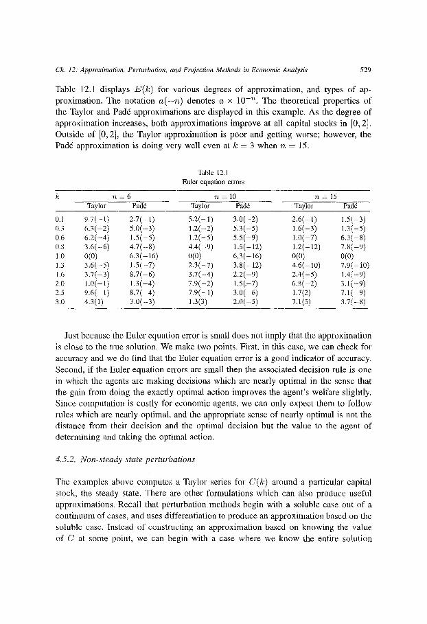
Judd and Guu [75] present Mathematica programs which compute arbitrary order Taylor and Pad6 expansions based on the derivatives of C at the steady state. Judd [74] shows that the 100 degree polynomial approximation to C is easily computed via a recursive formula. Table 1 displays the results for a variety of approximations. The assumptions are that u(c) = c('+'Y)/(1 + 7) and f ( k ) = pUVc~ with p = 0.04, 7 = - 2 , and c~ = 0.25. To evaluate the quality of the approximations, we compute a normalized, unit-free version of (21), which is the Euler equation error
E(k) = u ' r ( c (k ) ) C' ( k ) ( f - C(k)) + u ' (C(k) ) ( f ' ( k ) - p) (26)
8We drop arguments when they can be understood from context.
Ch. 12: Approximation, Perturbation, and Projection Me#uMs in Economic Analysis 529
Table 12.1 displays E(k ) for various degrees of approximation, and types of ap- proximation. The notation a ( - n ) denotes a x 10 -n . The theoretical properties of the Taylor and Pad6 approximations are displayed in this example. As the degree of approximation increases, both approximations improve at all capital stocks in [0, 2]. Outside of [0, 2], the Taylor approximation is poor and getting worse; however, the Pad6 approximation is doing very well even at k = 3 when n = 15.
Table 12.1 Eulerequation errors
k n = 6 n = 1 0 n = 1 5 Taylor Pad6 Taylor Pad6 Taylor Pad6
0.1 9.7(--1) 2 .7(-1) 5.2(-1) 3,0(-2) 2.6(-1) 1.5(-3) 0.3 6.3(-2) 5.0(-3) 1.2(--2) 5,3(-5) 1.6(-3) 1.3(-5) 0.6 6.2(--4) 1.5(-5) 1.2(--5) 5,5(-9) 1.0(-7) 6.3(-8) 0.8 3.6(-6) 4.7(-8) 4.4(-9) 1,5(-12) 1.2(-12) 7.8(-9) 1.0 0(0) 6.3(-16) 0(0) 6,3(16) 0(0) 0(0) 1.3 3.6(-5) 1.5(-7) 2.3(--7) 3.8(-12) 4.6(-10) 7.9(-10) 1.6 3.7(-3) 8.7(-6) 3.7(-4) 2.2(-9) 2.4(-5) 1.4(-9) 2.0 1.0(-1) 1.3(-4) 7.9(-2) 1.5(.-7) 6.8(-2) 3.1(-9) 2.5 9.6(-1) 8.7(-4) 7.9(-1) 3.0(-6) 1.7(2) 7.1(-9) 3.0 4.3(1) 3.0(-3) 1.3(3) 2.0(-5) 7.1(5) 3.7(-8)
Just becausethe Euler equation error is small does not imply that the approximation is close to the true solution. We make two points. First, in this case, we can check for accuracy and we do find that the Euler equation error is a good indicator of accuracy. Second, if the Euler equation errors are small then the associated decision rule is one in which the agents are making decisions which are nearly optimal in the sense that the gain from doing the exactly optimal action improves the agent 's welfare slightly. Since computation is costly for economic agents, we can only expect them to follow rules which are nearly optimal, and the appropriate sense of nearly optimal is not the distance from their decision and the optimal decision but the value to the agent of determining and taking the optimal action.
4.5.2. Non-steady state perturbations
The examples above computes a Taylor series for C(h) around a particular capital stock, the steady state. There are other formulations which can also produce useful approximations. Recall that perturbation methods begin with a soluble case out of a continuum of cases, and uses differentiation to produce an approximation based on the soluble case. Instead of constructing an approximation based on knowing the value of C at some point, we can begin with a case where we know the entire solution
530 K.L. Judd
and use that case to construct approximations. An example of this alternative is the continuum of problems
0 = C' (k , e) ( f ( k , e) - C(k , e)) + 7C(k , e) (p - f ' ( k , e)) (27)
where 3' is the constant relative risk aversion parameter, and
f ( k , e) = (1 - c)pk + ~k°~p/oe.
At e = 0, we hav~ a linear production function with a marginal product of capital equal to p, the pure rate of time preference; in this degenerate case, the solution is C(k , e) = pk, that is, consumption equals output. At all positive values for c, the production function is concave and the unique steady state is k = 1. Suppose that we are really interested in the e = 1 case where f is the standard Cobb-Douglas production function.
The first perturbation of (27) implies that for all k and e,
0 = Cke( f - C) + Ck(f~ - C~) + "TCe (p - A ) + "TC ( - f a t ) .
which at e = 0 and C = pk reduces to
o = C k ( A - + z C
and implies the solution
c (k, 0) = - ' - 7) + ( z p - p )k .
Continued differentiation will yield more terms which can be use in a Taylor series approximation for the Cobb-Douglas production function (c -- 1) case of the form
C ( k , l ) - C ( k , O ) + C ~ ( k , O ) + C ~ ( k , O ) / 2 + C ~ ( k , O ) / 6 + . . . . (28)
Note that this approximation is an approximation at all k, and theory tells us that it is good only for small c. To determine how good this approximation is for C(k, 1) we could substitute it into the Euler equation and check to see if the Euler equation errors are small. They often turn out to be acceptable, but we will see below that even if (28) does not solve (27) well, the C~(k, 0), C~(k ,O) , etc., functions can still turn out to be very useful.
Ch. 12: Approximation, Perturbation, and Projection Methods in Economic Analysis 531
4.5.3. Single-sector, stochastic growth
We next take the deterministic model above, add uncertainty, and show how to use the approximation to the deterministic policy function around k ss in the deterministic case to compute an approximate policy function in the model with a small amount of uncertainty. While the assumption of small shocks may seem limiting, it is sensible in many applications, such as macroeconomic and related financial analysis.
The stochastic problem is
{/o } V(k) = s u p E e -or u(c) dt ,
dk = ( f ( k ) - c)dt + ~ d z .
(29)
The Bellman equation becomes
0 = max [ -pV(k ) + u(c) + Vk(k) ( f (h) - c) + ec~ (k) Vkk (k)]. C
It is straightforward to show that C(k) solves
o - ~(k)~'"(C(k)) + ¢(k) ~"(C(k)) + ,y(k) ~'(C(k)) (30)
where
~(k) = ~ ( k ) [c'(k)] 2,
¢(k) = [f(h) - h(k) + ea'(k)] C'(k) + ecr(k) C"(k) ,
-y(k) = f ' (k) - p.
Formally, we are again looking for the terms of the Taylor expansions of C,
C(k, e) -- C(kSs, O) + Ck(kSS,0)(k - k ~ ) + C~(k~S,0)~
+ Ckk(k% 0)(k - k ~ ) 2 / 2 + C~k(k ~s , 0)~(k - k ~ )
+ C~(k ~,0)e2/2 + . . . . (31)
Before proceeding as before, we should note that the validity of these simple methods in this case is surprising. Note that (30) is a second order differential equation when e ~ 0, but that it degenerates to a first-order differential equation when e = 0. Changing e from zero to a nonzero value is said to induce a singular perturbation in the problem because of this change of order. Normally much more subtle and sophisticated techniques must be used to use the e = 0 case as a basis of approximation for nonzero c. The remarkable feature of stochastic control problems, proved by
532 K.L. Judd
Fleming [48], is that this is not the case here, that perturbations of e, the instantaneous variance, can be analyzed as a regular perturbation in e. 9
With Fleming's analysis in hand, we will now proceed. We assume that we know all the k derivatives of C at k = k 8s and e = 0. This is what the previous section on deterministic problems produced. We now move to computing C, by differentiating (30) with respect to e. When we impose the deterministic steady state conditions f ( k ss) = C(kS~), f ' ( k ~ ) = p, and c = 0, we arrive at a linear equation which implies that
I t l .r"¢ 2 C e - u t~ k +Ckk
u"Ck or(k) + a'(k) (32)
where all the derivatives of C are evaluated at k = k s8 and e = 0. Note that the solution for C, is a function not only of the deterministic steady state value of u, u t, and u", it also depends on u m, and Ckk, which in turn depends on fro. If u were quadratic, f linear, and ~r~(k) = 0, then (32) shows that C, = 0, as we expect from the certainty equivalence results for linear-quadratic control. Again, continued differentiation of (30) with respect to e and k leads to solutions for C~, C~k, Ck~,, etc. Judd and Guu [75] present Mathematica programs for computing these coefficients. They also show that the approximations are valid over a substantial range of values for e and k.
4.5.4. Dynamic programming
The optimal growth examples above are just special cases of dynamic programming problems. Albrecht et al. [1] showed that one could differentiate the Bellman equa- tion with respect to an exogenous parameter. Even the higher-order aspects of the computations above can be justified. Blume, Easley and O'Hara [14] discuss when dynamic programming solutions are smooth in the state variables. Bensoussan [10] also provides a general treatment.
4.5.5. Adjustment cost models
The problems above were based essentially on first-order conditions. We can apply perturbation methods to other problems which are not as simple. Dixit [44] studied the dynamics of models where a controller wants to keep the state of a system close to some optimal value and incurs a fixed adjustment costs whenever he adjusts the state. This leads to (S, t, s) rules; that is, when the state moves up to S or down to s the controller incurs the adjustment cost and pushes the state to a target t.
9A more modem analysis of this problem relying on viscosity methods instead of probabilistic methods is in Fleming and Souganides [49]. Their approach is also more general, possibly including distorted economies.

Ch. 12: Approximation, Perturbation, and Projection Methods in Economic Analysis 533
There are many models which fit this description, but they seldom have analytical solutions to the problem of determining S, s, and t in terms of structural parameters. Dixit used perturbation methods to derive algebraic formulas for S and s in terms of structural parameters. He also demonstrates that first-order approximations yield very good approximations when the adjustment cost is empirically reasonable. On the qualitative side, he makes rigorous the fact that the region of inaction, S - s, is quite large for small variance; more precisely, he proves a fourth-power law which states that S - s e( c 1/4 when the adjustment cost is c. This result is quite important since it says that the region of inaction is quite large relative to the cost for small costs. Dixit [44] discusses a number of applications of this result. This is an excellent example of how one can use the perturbation method to get an analytically simple rule of thumb which provides important intuition about a problem.
4.5 .6 . S t o c h a s t i c e q u i l i b r i u m ana lys i s w i t h o u t P a r e t o e f f ic iency
Many equilibrium problems do not reduce to optimal control problems, such as dy- namic equilibria with taxation or money. While the discussion above concerned an optimal control problem, the same methods can be used to study the behavior of an economy distorted by taxation. The basic fact is that near the deterministic steady state, the linear approximation to the law of motion in the stochastic model is
d x = A ( x - ( x ~ - A ) ) d t + 52 d z (33)
where A is the linearization of the deterministic model and S is the covariance matrix of the shocks to the state. In the deterministic model, x ss is the target state and A "pushes" the state towards the target. This expressions shows that the linear approximation to the stochastic model involves the same linear law of motion locally but with a new target, where the adjustment A arises due to certainty nonequivalence.
With this observation, Balcer and Judd [4] studied the effects of taxation in a simple capital accumulation model where (33) reduces to
dk = A(k - (k ss - A))dt + Z d z (34)
where ~ is the negative eigenvalue of the linearization of the dynamic system de- scribing the taxed equilibrium (similar to (10)). Therefore, the effects of taxation on business cycle fluctuations reduce to its effect on ~. They show how the level and the composition of the effective tax rate affect important business cycle statistics.
One can also compute equilibrium utility under distortions. If we have a tax of ~- on all income but have all revenues rebated in a lump-sum fashion, the equilibrium value function is
. v (k ) = ~(c(k)) + Vk(k) (f(k) - C ( k ) ) + c~ (k)Vkk(k). (35)
534 K.L. Judd
An optimal policy chooses consumption to maximize the fight-hand side, but the equilibrium policy under taxation does not. To see the difference, recall that the de- terministic steady state is the k ~- which satisfies i f ( U ) = p/(1 --r) in the deterministic case. Then, differentiating (35) with respect to k yields
pVk(k) = u'Ck + Vk(k) (f f - Ck) + Vkk(f -- C) (36)
which reduces at k ~- to
u ' - V k = V k ( f ' - p ) Vk r Ok = P C'k 1 - ~-
which shows that the social marginal value of capital deviates from marginal utility of consumption when the tax rate is not zero.
This fact is important when we come to evaluate the impact of uncertainty on the equilibrium value function. Differentiating (35) at e = 0 and k = k ~- we find
pYo = ( u ' - v k ) c , +~Vkk (k ) (37)
which implies that the true first-order approximation to V around the deterministic steady state is
V(k , ~) - (k - k ' )Vk + ~((~' - Vk)C~ + ~ Vkk(k))/p. (38)
This shows that the impact of uncertainty on the equilibrium value function depends on the degree of certainty nonequivalence, C,, when the tax rate is nonzero, and that dependence increases with increasing taxation. This is an example of a question where certainty-equivalent methods of approximating a stochastic economy will not produce reliable, first-order accurate answers.
4.5. 7. Multidimensional, high-order approximations
The examples explored above have only one dimension. These methods can be ex- tended to multidimensional problems, yielding high-order approximations to multidi- mensional problems. Bensoussan [10] discusses these problems for the finite-horizon case, and Judd [74] presents these procedures for the infinite-horizon case. A nontrivial difficulty in dealing with the higher-order approximations is the messy notation asso- ciated with multivariate versions of Taylor's theorem. Judd [74] extends the Einstein tensor notation, which was introduced to drastically simplify expressions in general relativity theory, to make these higher-order approximation techniques in optimal con- trol contexts more tractable. Judd [74], following Fleming [48], further extends the multidimensional case to include uncertainty. The basic fact is that all the higher- order terms of the Taylor series expansion, even in the stochastic multidimensional
Ch. 12: Approximation, Perturbation, and Projection Methods in Economic Analysis 535
case, are solutions to linear problems once one computes the first-order term in the state variables. This indicates that the higher-order terms are easy to compute. Initial experiments indicate that they are also good approximations well beyond the steady state values. These procedures have not been exploited much, but can be obviously applied to problems in the real business cycle, finance, public finance, and dynamic general equilibrium literatures.
The other development is the work of Fleming and Souganides [49]. They derive asymptotic results for problems written in viscosity form. One advantage of these problems is that they can handle infinite-horizon problems, whereas the results de- scribed in Bensoussan are proven mostly for finite-horizon cases. While discussing viscosity, a relatively recent advance in nonlinear partial differential equations, is be- yond the scope of this paper, we should note that these methods surely cover the equations which arise in dynamic programming, and might generalize to cover equi- librium problems.
4.5.8. Dynamic games
Perturbation techniques can also be used to analyze dynamic games. Because of the notational burden of a formal treatment, I will here just give the basic idea behind the perturbation approach. Suffice it to say here that we are discussing dynamic game equilibrium concepts which can be written as solutions to ordinary or partial differential equations, or some similar system of functional equations.
As with any perturbation method, we begin with a "point" (possibly in a function space) where we know the solution. In game theory, such cases do arise. For example, suppose that we have two players who each influence their own state variables, but that the payoff functions and the laws of motion are such that neither player is affected by the actions of the other. This would, for example, be the case of two differentiated duopolists where the cross-elasticity of demand is zero, and the state variable of the game is the vector of the firm's capital stocks. Then the equilibrium of such a "game" is trivial, reducing to an optimal control problem for each player. Using the techniques above, we can compute local approximations for each player's strategy around steady states of the degenerate game.
Now suppose that the payoffs and/or laws of motion are slightly perturbed so that each player now cares about the other's actions. By differentiating the functional equations which characterize equilibrium with respect to the perturbation parameter and imposing the implicit function theorem and Taylor's theorem, we will be able to compute how equilibrium is affected by the alteration.
Another kind of starting point is to specify a game with general interactions, but make some parametric assumption such that the players have no interest in the dy- namics. This is the case when the interest rate is infinite. In such cases, the dynamic game reduces to a static game and, in equilibrium, neither player expends any effort to affect the future. With this degenerate case in hand we can then compute expansions
536 K,L. Judd
in the inverse of the interest rate to determine what happens as the firms begin to care about the future. There are two examples of papers using these methods.
Judd [69] applied Theorem 4 to a patent race model. He assumed a duopoly model where the players had two kinds of research strategies and it is necessary to complete a sequence of steps. Analytic solution of such a general problem is clearly impossible. He began by assuming that the patent race had a zero prize for the winner, which, of course, implies a Nash equilibrium of no effort. This is also equivalent to the infinite interest rate case. He then proved local existence of equilibrium as well as constructed local linear and quadratic approximations.
Budd et al. [23] contains the most complex perturbation analysis of a dynamic game. They analyzed a stochastic market share duopoly game. Specifically, current profits for each firm is a function of firm one's market share, s, which is the state of the game. Each player expends effort to increase his share, which moves stochastically. The result is a stochastic dynamic game. The two degenerate cases they use are the infinite interest rate case and the case of infinite instantaneous variance of random movements in s. In these cases the firms either don't care about future market share or essentially have no control over future market share, implying a Nash equilibrium of zero effort. They compute asymptotic expansions in the inverses of the interest rate and the disturbance variance. With these expansions they are able to examine the dynamics of competition, determining when, for example, the laggard firm will work hard to catch up, when the leading firm will work hard to keep its advantage, etc.
There have been few applications of perturbation methods to game analyses thus far, but they do indicate the potential of the method. Srikant and Basar [118] develops regular perturbation methods for a large class of dynamic games different from those examined in Judd and Buddet al. Given the general applicability of these methods, the increased interest in dynamic econometric analyses, and the difficulties of game theory computation, one suspects that these procedures will become increasingly popular.
4.5.9. The macroeconomic "Linear-quadratic approximation"
The perturbation methods described have been used to approximate a wide variety of optimal control and economic equilibrium problems, and can be used much more extensively. While many macroeconomists have also studied stochastic growth models, many have eschewed the procedures above and instead use ad hoc procedures which replace nonlinear growth models with hopefully similar linear-quadratic models. Since the latter strategy bears some similarity to perturbation methods and often uses similar terminology, we will next describe it and discuss the many differences between it and perturbation methods.
As discussed in Magill [93] and Kydland and Prescott [84, 85], one basic idea is to replace a stochastic nonlinear control problem with a "similar" linear-quadratic control problem which "approximates" the nonlinear model, and then apply linear-
Ch. 12: Approximation, Perturbation, and Projection Methods" in Economic Analysis 537
quadratic methods to solve the model) ° This procedure is described precisely in McGrattan [95]. 11 She takes the nonlinear stochastic optimal control problem
V(z0) -- m a x E tTr(u,x) , U t
z~+l = g(z~, ut , ct)
(39)
where x is a vector of state variables, u is a vector of controls, and 7c is concave. She
solves for the steady state of the deterministic version of (39), and replaces (39) with
the linear regulator problem
! V(xo) =-- max E /3 t (xtQxt + u~Rut + 2x~Wut) ,
Ut
Xt+l = Axt + But + Cet
(40)
where x~Qx + u~Ru + 2x~Wu is the second-order Taylor expansion of 7r, and
A x + Bu is the first-order Taylor expansion of 9, both taken at the deterministic
steady state. 12
The linear-quadratic procedure outlined in McGrattan [95] differs from the pertur-
bation method in its approach, objective, and results. Despite using the term "lineal"
approximation," the objective is not to compute a locally valid Taylor series for the
equilibrium behavior rules. In fact, this procedure may produce an "approximation"
which differs substantially from the Taylor series produced by perturbation methods. This is immediately seen by applying it to (29): f " ( k ss) appears in the solution to
C~(k ~) in (25) but appears nowhere in (40) after we apply McGrattan's procedure
to (29); therefore, the linear decision rule computed by McGrattan's method applied
to (29) would not be the linear approximation of the true decision rule at the steady
state, (22), even in the deterministic model. In fact, those who use this procedure
raThe procedure described here is applicable only to optimal control problems, and those equilibrium problems which reduce to optimal control problems.
l IWhile many have used the "linear-quadratic" method, McGrattan's is the only precise statement of the procedure for the general discrete-time multidimensional control problem which I have seen in the published literature. The Magill procedure is the correct procedure, differs from McGrattan, but has been largely ignored.
12Kydland and Prescott use a slightly different procedure. They choose linear rules which satisfy the Euler equation at a collection of points near the steady state, where the collection is determined by the variance of the shocks. In this respect, their procedure is similar to the projection method we discuss below. They comment that in the case they examine, the differences are slight, but there is no reason to believe that this is always true. I include their procedure here since their stated goal is to simplify "the determination of the equilibrium process by reducing it to solving a linear-quadratic maximization problem".

538 K.L. Judd
generally make no claim that they are computing the linear approximation of the true decision rule.
If one were to use investment instead of consumption as the decision rule in (29) then the result from McGrattan's procedure does yield the true linear approximation in many cases (further work is needed to see how general this fact is). This does not say that McGrattan's procedure is correct. Instead it points out an undesirable sensitivity to economically inessential details in the formulation of the problem. In contrast, perturbation methods are not sensitive to such changes.
No matter how one proceeds, the approach in McGrattan, Magitl, and Kydland and Prescott, makes no adjustment for variance. The approximation is a certainty equivalent approximation even though the true problem is generally not certainty equivalent. At best, this procedure computes the first two terms of (31) above but drops the third and later terms. The result is only half of the true linear approximation at the deterministic steady state since the approximation includes the linear Taylor expansion term for the state variables but excludes all Taylor expansion terms for the variance terms. Multidimensional generalizations of the rules computed in Judd and Guu [75] have no such problems.
This intuitive way of approaching the problem can lead to some conceptual prob- lems in thinking about approximations. The linear-quadratic intuition behind (40) says to replace a nonlinear problem with a similar linear-quadratic problem because the latter is solvable. Suppose that you wanted a higher-order approximation of the optimal decision rule. This approach suggests that the way to compute a quadratic approximate decision rule would be to take a third-order polynomial approximation of the objective around the deterministic steady state and solving exactly the resulting cubic optimal control problem. Of course, there is no exact solution in general for third-order problems, making it appear difficult to compute a quadratic approximation to the decision rule. In contrast, the perturbation methods described above show that the higher-order terms are in fact easy to compute.
Christiano [30] adopts a different approach to the "linear-quadratic" approach. He writes down the Euler equations for the nonlinear model in the form (18), and then linearizes these equations around the steady state to create a linear system of the form (19). Two comments are in order. First, this essentially reduces the problem to a calcu- lus of variations problem. Since this cannot be done for all optimal control problems, this approach is limited. However, it is justified by the stable manifold theorem. Sec- ond, he also imposes certainty equivalence on his approximation to stochastic models. Therefore, he also ends up with only a "half-linear" approximation.
Dotsey et al. [45], Christiano [30] and McGrattan [95] have documented the qual- ity of some implementations of the macroeconomic linear-quadratic approach. The results follow what one would expect from the perturbation analysis. The Christiano and McGrattan implementations of the linear-quadratic method do fairly well when it comes to modeling movements of quantities, but not as well with asset prices. This
Ch. 12: Approximation, Perturbation, and Projection Methods in Economic Analysis 539
is expected since perturbation methods show that the linear approximation of quan- tity movements depend on only linear-quadratic terms whereas asset pricing move- ments are more likely to involve higher-order terms. In particular, the extra terms produced in Judd and Guu [75] show that the deviations from certainty equivalence depend on higher-order derivatives of the utility function. The linear-quadratic ap- proximation also does less well as the variance of the productivity shocks increases since the linear-quadratic approach ignores the effects of the variance on the decision rules.
The linear-quadratic scheme in (40) is used to solve for equilibria which solve a social planning problem. Macroeconomists have devised complex iterative schemes to compute equilibria of distorted economies. They also revolve around linear-quadratic approximations of the individual agents' problems (see, for example, Cooley and Hansen [37]). These procedures are offered without any rigorous justification, and offer no reason why they should be used instead of the earlier linearization methods derived from standard mathematical methods. As pointed out above, the standard perturbation methods used by Laitner, Judd, Bovenburg, and described in Stokey and Lucas will compute first-order valid linear approximations in nonlinear equilibrium models, and do so in a nonrecursive, hence much faster, fashion.
Furthermore, the problems with this macroeconomic approach are even greater when dealing with distorted models. These approximations also ignore the impact of variance. The point of many of these exercises is to compute the welfare effects of various policies. This requires the computation of an equilibrium value function. We saw above that the first-order approximation to such functions, (38) includes the deviation from certainty equivalence when taxes are present. Therefore, their compu- tations of utility are not reliable. Another example of the inadequacy of an informal approach is in Chari et al. [27]. They show that the resulting "linear approximation" does poorly relative to a global nonlinear procedure. Since they do not take an explicit perturbation approach (that is, formulate it as an application of the implicit function theorem or one of its generalizations, and compute an appropriate number of terms), this is not evidence against the use of perturbation methods, only against the informal approach they use.
4.5.10. Linear model computation
The linear approximation approach could also be used, but has been overlooked, when it comes to the analysis of linear-quadratic models. The idea is simple: if one has a model with a deterministic steady state and globally linear equilibrium behavioral rules, then the linear rules which are locally valid near the steady state are the globally valid rules. All of the perturbation methods outlined above are direct, noniterative, methods in contrast to the complex, iterative procedures often used by economists to solve linear dynamic economic models.
540 K.L. Judd
5. Bifurcation methods
Sometimes we will want to compute an approximation to an implicitly defined function at a point where the conditions of the Implicit function theorem do not hold, in particular when Hy(xo, yo) is singular. In some cases, there is additional structure which can be exploited by bifurcation methods, to which we now turn.
Suppose that H ( x , e) is C 2. One way to view the equation H ( x , e) = 0 is that for each e it defines a collection of x which solves the equation. We say that e0 is a bifurcation point if the number of solutions to H ( x , e) = 0 changes as c passes through co. Two situations are summarized in the following theorem.
THEOREM 5 (Bifurcation theorem). Suppose H ( x , O) = O for all x, where H : R 2 -+ R. Furthermore, suppose that
H (xo,O)=O =H,(xo, O),
f o r some (xo, 0). Then, /f Hcc(xo, 0) ~ 0, there is an open neighborhood A/" of (x0, 0) and a function h(e), h(e) 7 ~ O for e ~ O, such that
H ( h ( e ) , e ) = 0 on A f
and H ( x , e) is" locally diffeomorphic to e ( e - x ) or e (e+x) . Otherwise, i f H, , (xo , O) = 0 ¢ H ~ , (x0, 0), then there is an open neighborhood .Af of (x0,0) and a function h(e), h(e) 7/= O fo r e ~ O, such that
H ( h ( , ) , , ) = 0 on N
and H ( x , e) is locally diffeomorphic to e 3 - xe or e 3 + xe. In both cases, c = 0 is a bifurcation point.
It may seem that Theorem 5 has limited applicability given its low-dimension character. Fortunately, there is a procedure, the Lyapunov-Schmidt method, which is used to transform high dimension (even infinite dimension) problems into appropriate low-dimension problems at which point one applies the procedures above. This greatly increases the applicability of this approach.
Theorem 5 also seems limited in that H has domain R 2. Theorem 5 generalizes to H : R n+1 --4 R ~. Furthermore, the Bunch theorem (see Zeidler) generalizes the bifurcation methods in Theorem 5 to allowing both x and e to be in Banach spaces. Space limitations prevent our discussing these generalizations here, but below we will see that economic applications are obvious.
There are many kinds of bifurcations; the simple ones in Theorem 5 are referred to as the transcritical and pitchfork bifurcations. Another, more complex, bifurcation

Ch. 12: Approximation, Perturbation, and Projection Methods in Economic Analysis 541
which arises naturally in economics is the Hopf bifurcation. We present the statement in Benhabib and Nishimura [9].
THEOREM 6 (Hopfbifurcation). Suppose that {c = [i'(z,#), z E G C R n, # E [-c, c]C R, F E C k. Suppose that there exists stationary solutions, that is, for I~1 < c, there is ~(#) such that F(2(#), #) = O. Suppose that the Jacobian Fx(2(#), #) has a parametric pair of eigenvalues which can be expressed as a(#) 4-/3(#)i where a(O) = O, /3(0) ¢ O, and a'(O) ¢ O. Then there exists a family of parametric so- lutions z(t , e) and #(e) of ~c (t, e) -- F(z( t , e), t~(e)) such that z(t,O) = "z(O) but z( t ,e) 7 ~ Y(#(e))for e ¢ 0. Furthermore, #(c) is C k- ' and the period of the cycle is 27r/ t/3(0)t.
The result stated above is just a first-order result; higher order approximations are available. There are also conditions which guarantee that the periodic solutions are stable orbits. There are further generalizations of the Bifurcation Theorem which cov- ers cases where there are many nondegenerate branches passing through a bifurcation point. Such cases may correspond naturally to multiple equilibria in economic models. For a more complete discussion of these issues see Zeidler [128], Chow and Hale [34] and Golubitsky and Schaeffer [53].
5.1. Applications of the Hopf bifurcation to dynamic economic theory
The Hopf bifurcation has been extensively used to study the possibility of deterministic cycles in economic models. Benhabib and Nishimura [9] explored the possibility of cycles in multisector growth models. They showed how to use the Hopf bifurcation to check for the presence of Hopf bifurcations and offered plausible numerical examples of Hopf bifurcations in optimal growth models. Zhang [131] presented a simplified version of this analysis and also showed how to compute expressions for the period of such cycles and how to check their stability.
The Hopf bifurcation has also been used in Industrial Organization theory. Feich- finger [46] used the Hopf bifurcation in a dynamic model of advertising to argue that cycles in advertising expenditure were quite plausible. The Hopf bifurcation has also been used to analyze general equilibrium with financial imperfections. The theme of these papers is that while the equilibrium dynamics of an economy may be stable with perfect capital markets, capital market imperfections may lead to more complex dynamics. Again, the Hopf bifurcation is used to demonstrate the existence of stable cycles. These papers include Franke [50], who investigated a Keynes-Wicksell model with adaptive expectations for inflation and found that periodic orbits were possible.
There are possibly many other applications of the Hopf bifurcation. Most dynamic analyses examine only the steady state, not its local dynamic structure. At the least, one can check the local linear structure to see if the number of stable and unstable eigenvalues is consistent with local asymptotic stability. Since stable cycles are often

542 K.L. Judd
associated with unstable steady states, the presence of too many unstable eigenvalues should lead an analyst to check for the possibility of a nearby Hopf bifurcation. Since this checking is purely an algebraic exercise, easily done by symbolic computation methods, such checks should become standard.
5.2. Gauge functions
The methods described above, commonly referred to as regular perturbations, compute Y~'~i=l aieL are where we expansions of the form ~ " There many cases will want to
compute different expansions. In general, a system of gauge functions is a sequence of functions, {Sn(e)}~°°__ 1, such that
lim ~n+l(e) _ 0. ~-~o O~n (~)
An asymptotic expansion of f (x) near x = 0 is denoted
f (x) ~ f(O) + ~ a i S i ( x ) i=1
where, for each n,
lim f (x) - ( f (0) + Y~-a ai 5~(x)) = 0. • -~o 6~(x)
In regular perturbations, the sequence of gauge functions is 5k(e) = e k. Another example of a gauge system is 5k(c) = c k/2. In many problems, the main task is determining the correct gauge system. The next sections present examples of this more general problem.
5.3. Bifurcation applications to stochastic modelling
Whereas the Hopf bifurcation is useful in analyzing deterministic systems, the simpler pitchfork and transcritical bifurcations examined above in Theorem 5 can be used to study stochastic problems. In this section, we will illustrate this with two examples. First we will discuss the details of a simple portfolio problem. Second, we will discuss a much more sophisticated application.
5.3.1. Por(olio choices with small risks
Suppose that an investor has W in wealth to invest in two assets. The safe asset yields R per dollar invested and the risky asset yields Z per dollar invested. If a proportion

Ch. 12." Approximation, Perturbation, and Projection Methods in Economic Analysis 543
co of his wealth is invested in the risky asset, final wealth is Y = W((1 - c o ) R + c o Z ) .
We assume that he chooses co to maximize E { u ( Y ) } for some concave utility function ~(.).
One way in which economists have gained insight into this problem is to ap- proximate u with a quadratic function and solve the resulting quadratic optimization problem. It is argued that this is valid for small risks. The bifurcation approach allows us to examine this rigorously. We first create a continuum of portfolio problems by assuming
= R + e5 + e2¢c.
At e = 0, Z is degenerate and equal to R. If 7r > 0, we model the intuitive case of risky assets paying a premium. Note that we multiply £ by e and 7r by e 2. Since the variance of ez is e 2 a2, this models the observation that risk premia are the same order as the variance.
Judd and Guu [77] applied the Bifurcation theorem to this problem, producing a procedure which involves solving only linear equations and which can be used for noncompact distributions. We will briefly outline their analysis. The first-order condition for co is (assuming W = 1)
o - E{~ ' (R + co(~z + ~2.)) (z + ~ ) } - G(co, ~). (41)
We want to analyze this problem for small e. We cannot apply the implicit function the- orem since 0 = G(co, 0) for all co implying that co is indeterminate at e_ = 0. Since we want to solve for co as a function of e near 0, we first need to compute which of these co values is the "correct" solution to the e = 0 case; specifically, we want to compute
lira t" \ coo ~- co<e).
Implicit differentiation of (41) implies
0 = G~ co' + G~. (42)
Differentiating G we find
Ge = E { u " ( Y ) (coz + 2coeTr) (z + eTr) + u '(Y)zr},
G~ : E{~" (9 ) (z + ~)2~}.
At e = 0, G~ = 0. co'(0) can be well-defined in (42) only if G~(co, 0) = 0 also. Therefore, we look for a bifurcation point, coo, defined by 0 = Ge(coo, 0). At e = 0, this reduces to 0 = u"(R)coo~z 2 + u'(R)Tr, which implies
c o o - ~ ' ( R ) ~z 2"

544 K.L. Jb!dd
This is the simple portfolio rule indicating that co is the product of risk tolerance and the risk premium per unit variance. If coo is well-defined, then this must be its value. Since the conditions of tile Bifurcation theorem are satisfied at (coo, 0), there is a function co(e) which satisfies (41) and goes through (w0, 0).
Note that this is not an approximation to the portfolio choice at any particular variance. Instead, coo is the limiting portfolio share as the variance vanishes. Some authors treat this as an approximation to the true solution, co(e), for small c. That, however, is not the case. If we want the linear approximation of co(e) at (coo, 0), we must go one more step since the linear approximation is co(e) - co(0) + e w'(0). To calculate co'(O) we need to do one more round of implicit differentiation. Differentiat- ing (42) with respect to c yields 0 = G ~ colw ~ + 2G,o~ co! + G~oco" + G~. At (coo, 0), G~ = u'"(R)co~ E{z3}, G ~ = O, G ~ = u"(R) E{z2}. Therelbre,
1 ,.'"(R) E{z 3} co'(o)-- 2 E{z2} cog
This formula tells us how the share of wealth invested in the risky asset changes as the riskiness increases, highlighting the importance of the third and second derivatives of utility and the ratio of skewness to variance. If the distribution of the risky asset is symmetric, then E { z 3 } = O, and the constant coo is the linear approximation of co(e). This is also true if urn(R) -=- O, such as in the quadratic utility case. However, if the utility function not quadratic and the risky return is not symmetrically distributed, then co~(0) ~ 0, and the linear approximation is a nontrivial function. Note that this says that a linear approximation to co(e) requires a cubic approximation to the utility function and third moments of ~. This fact, also demonstrated in Samuelson [114], shows how the simple approach of using only a quadratic approximation to the objective function does not produce a valid linear approximation for co(e). The advantage of the bifurcation approach demonstrated here is that the structure of the problem indicates exactly what information is needed.
Samuelson [114] earlier analyzed this problem in a less formal fashion. Also, his formal analysis was limited to Z with compact distributions, that is, random variables whose support goes to a point as e goes to zero, a detail which substantially limits practical interest. The perturbation arguments used above make no such restriction. While the Samuelson method worked in this example, using Theorem 5 allows us to proceed in a more general fashion, and provides the necessary formal justification for these calculations.
One example of where the true problem has a bifurcation structure and standard linear approximation procedure is unacceptable is Huffman [63]. Huffman examined an overlapping generations model of capital accumulation, and tried to examine the impact of a business cycle shock on asset trading. He computed the deterministic steady state and computed the impulse function for individual wealth and asset trading arising from unanticipated shocks to endowments and output. Since this was all done
Ch. 12: Approximation, Perturbation, and Projection Methods in Economic Analysis 545
in an otherwise deterministic, perfect foresight model, the tacit assumption, appropriate for such models, was that equity was the only traded asset. However, Huffman then interpreted the impulse functions from the deterministic model as impulse response functions for a stochastic model, where all agents know that these shocks occur frequently. In the stochastic case, there would also be demand for trade in bonds as well as equity, and business cycle shocks would generate disturbances to bond holdings and equity holdings. This was ignored by Huffman, who implicitly assumed that even in the stochastic model the only asset was equity. Such a capital market imperfection will have important impacts on the predicted asset trading, and is not an appropriate approximation assumption; just because one of the deterministic equilibria has no bond trading does not mean that the absence of bonds is an appropriate approximation for the stochastic model, even one with shocks with small variance. The importance of including bond trading into the analysis depends on the question being investigated. It is likely that the welfare loss is small when the variance is small. However, including bond trading could have substantial impact on the volume of trade in assets. A bifurcation approach can include bonds and equity and analyze such trade.
5.3.2. Bifurcation and sunspots
A particularly sophisticated application of bifurcation techniques appeared in Chi- appori et al. [29]. They analyzed the existence of stationary sunspot equilibria near steady states of overlapping generations model of arbitrary dimension. They show that when a steady state has indeterminate local deterministic dynamics, i.e., there exists a continuum of perfect foresight paths converging to the steady state, then there exists a continuum of sunspot equilibria which have support in neighborhoods of the steady state. They also are able to determine the possible qualitative character of the sunspot equilibria. This paper displays a very sophisticated and rich application of the ideas behind Theorem 5. These methods will also allow researchers to assess quantitative aspects of sunspot equilibria.
6. Asymptotic expansions of integrals
In economic and econometric problems, integrals frequently take the form
1()~) ==- JD e-Xg(x) f (x ) dx (43)
where A is a large parameter. Simply differentiating (43) with respect to A at A = ec will not work here. Laplace's method provides a useful way to approximate (43). The basic idea is that the major contribution of the integrand is at the minimum of 9(x).
546 K.L. Judd
Suppose g(x) is minimized at x = a. For large A, if x ¢ a then e-)'.q(x) << e-)W(a). As long as f ( x ) does not offset this for Ix - a I >> 0, I(),) is determined largely by the behavior of the integrand, e-'Xg(x)f(x), for x near a.
The one-dimensional case is easy to state. Assume that g and f satisfy the asymp- totic series
OO g(x) ~ g(a) + E ai(x - a) i+t',
i=o
OO f ( x ) "-' E b i ( x - a) i + a - I .
i=0
Under modest assumptions (see Wong [126], or Bleistein and Handelsman [13]) if
the integral I(A) = f : f ( x ) e -)'9(~) dx converges absolutely for sufficiently large A, and if g is minimized on [a, b] at a, then
I(A) ~ e -)'g(a) F A(i+cO/t ~ i=o
(44)
where .U(A) _= f0 ~ e - ~ x ;~-1 dx is the gamma function, and the ci depend on the ai and bi. In particular
bo ( bl c O -- c~/l ~ ~ Cl =
#a o #
(o~ +#2aol)al bo) ao(O~+l)/..
To compute these coefficients and others one essentially expands the integrand in terms of A and matches like powers. 13 One of the byproducts of this theorem is the construction of an integrand which is close to e -xg(~) f ( x ) but also integrable. This approximation to the integrand is then integrated to produce Laplace's approximation. Note that the gauge functions of A in (44) depend on the asymptotic expansions of f and g.
One elementary application of Laplace's method is Stirling's formula for n!. Recall that n! = F ( n + 1). We would like to approximate F(n) for large n. To use Laplace's method, let x = yA; then
~0 °° F(A) = A ~ e-)'(Y-lnY)y -1 dy.
The minimum of y - In y is at y = 1. Break the integral into two integrals over [0, 1] and [1,o c), and add the two one-sided approximations to get the two-term approximation
(1) ff()~) ~ ~ /@-l/2e-A 1 q- 1 ~ "
13Bender and Orszag gives an intuitive presentation of this procedure.
Ch. 12: Approximation, Perturbation, and Projection Methods in Economic Analysis 547
Stirling's formula is just the one-term expansion, n! ~ v/-2-~(n + l)n~-U2e-(n+l). While the operating assumption in Laplace's approximation is that A is a "large"
parameter, practical use of such methods rely on what "large" means quantitatively. Fortunately, these expansions may do very well even when A is actually small. For example, Stirling's approximation for 1! is 0.9595 and the two-term expansion yields 0.9995.
There is a multidimensional extension of Laplace's method. Suppose D C R ~, f , 9 E C2[D]. Suppose the minimum of 9(x) for x c D is achieved at x0 in the interior of D. Then the leading term of the expansion is
e_~g(~o) ( ~ ) n/2 Z(,~) - - [ N i l / 2 f ( x o )
where H -~ (gx~xj) is the Hessian of 9 at x0. Higher order terms can also be computed. While computing higher-order terms would be very tedious, symbolic languages such as Mathematica, Maple, and Macsyma, are ideally suited to do this.
6.1. Econometric applications of asymptotic methods
Asymptotic methods in econometrics are essentially perturbation methods where the properties of an estimator are computed in terms of the size of the data set and the expansion is around the case of an infinite sample size. In some cases, the asymp- totic problem can be handled by relatively simple procedures, such as Edgeworth expansions.
In other cases, the full power of Laplace's method is needed to compute asymptotic properties of statistics. In this case, the integral is the likelihood function, and it is written in the form (43) where the parameter ~ is the sample size. Phillips [104] used Laplace's method to approximate small sample marginal densities of instrumental variables estimators. Ghysels and Lieberman [52] use Laplace's method to compute small sample biases which arise from using filtered data in dynamic regressions. Laplace's method has been more popular among statisticians; see the citations in [52]. Holly and Phillips [62] use the related saddlepoint procedure. These methods work well, but are not often used, possibly because their implementation requires much algebra. One suspects that a more intensive use of symbolic computational tools would make them more accessible.
6.2. Theoretical applications of Laplace's method
While the theoretical applications of asymptotic methods for evaluating integrals are few currently, they are likely to increase. Brock [ 19] discusses where Laplace's method
548 K.L. Judd
is useful in evaluating statistical mechanical systems adapted to economic issues. As this modelling approach matures, it is likely that Laplace's method and related asymptotic procedures will be quite useful.
7. The mathematics of L p approximations
We will often want to approximate functions over a broad range of values with relatively uniform accuracy. In this case, we turn to L v approximations. L p approxi- mations finds a "nice" function 9 which is "close to" a given function f in the sense of a L p norm. To compute an L v approximation of f , one ideally needs the entire function, an informational requirement which is generally infeasible. Interpolation is any procedure which finds a "nice" function which goes through a collection of prescribed points. When using interpolation, the objective is to assure that if the data comes from a function 9 then the interpolant is close to 9. Regression lies between L 2 approximation and interpolation in that the amount of data used exceeds the number of free parameters, producing an approximation which "best" fits the data. In all cases, we need to formalize the notions of "nice" and "close to".
7.1. Orthogonal polynomials
We will next use basic vector space ideas to construct representations of functions which will lead to good approximations. Since the space of continuous functions is spanned by the polynomials, x n, it is natural to think of the ordinary polynomials as a basis for the space of continuous functions. However, recall that good bases for vector spaces possess useful orthogonality properties. We will develop those orthogonality ideas to construct orthogonal polynomials.
DEFINITION 7. A weighting function, w(x), on [a, b] is any function which is positive and has a finite integral on [a, b]. Given a weighting function w(x), we define an inner product on integrable functions over [a, b]:
jfa b (f, 9) = f (x) 9(x) w(x) dx.
The family of polynomials {~n(x)} are mutually orthogonal with respect to the weighting function w(x) if and only if
{~,,~, ~ ) - - 0 , n ¢ m .
There are several examples of orthogonal families of polynomials, each defined by a different weighting function and interval. Some common ones useful in economics
Ch. 12." Approximation, Perturbation, and Projection Method9 in Economic Analysis 549
are Legendre, Chebyshev, Laguerre, and Hermite polynomials. Legendre polynomials assume w(x) = 1 on the interval [ -1 , 1]; the nth Legendre polynomial is
( - 1 ) n d ~ Pn(X) =--- 2nni dx n [(1 - x 2 ) n ] .
The Chebyshev polynomials arise from w(x) = (1 - X2) -1/2 on [--1, 1]; the nth Chebyshev polynomial is
Tn(X ) ~ C O S ( n C O S -1 X).
The Chebyshev and Legendre polynomials are useful in solving problems which live on compact sets since a linear change of variables will transform in compact interval into [ -1 , 1]. The Laguerre polynomials correspond to w(x) = e - x on [0, cxz); the nth member is
e x d n Ln(x) =- n! dx n (xn e-x)"
Laguerre polynomials are useful when one needs to approximate time paths of vari- ables in a deterministic analysis. Hermite polynomials arise from w(x) = e -~2 on ( - o c , ec); the nth member is
Hn(x) - ( - l ) n e ~2 dn d z ~ (e-X2) •
Hermite polynomials are used to approximate functions of normal random variables.
7.2. Least-squares orthogonal polynomial approximation
Given f(x) defined on [a, b], one approximation concept is least-squares with respect to the weighting function w(x). That is, given f(x), the least-squares polynomial approximation of f with respect to weighting function w(x) is the degree n polynomial which solves
b
min fa (f(x) -p(x)) 2w(x) dx. deg(p) ~<n
In this problem, the weighting function w(x) indicates how we care about approxi- mation errors as a function of x. For example, if one has no preference over where the approximation is good (in a squared-error sense) then we take w(x) = 1. If one
550 K.L. Judd
cared more about the error around x = 0 we should choose a w(x) which is larger near 0.
The connections between orthogonal polynomials and least-squares approximation are immediately apparent in solving for the coefficients of p(x) in the least-squares approximation problem. If {~}~=1 is an orthogonal sequence with respect to w(x) ,
and we define ( f , g) - f:o f ( x ) g(x) w(x ) dx the induced metric is 11 f II2= - (f, f ) , the least-squares solution minimizes [1 f - p H, and can be expressed
; ( x ) =
i=0
Note the similarity between least-squares approximation and linear regression. The formula for p(x) is essentially the same as regressing the function f on n + t orthog- onal regressors; the coefficient of the ith "regressor", qoi(x), equals the "covariance" between f and the ith "regressor" divided by the variance of the ith regressor. This is no accident since regression is a least-squares approximation.
7.2.1. Chebyshev approximation
We will next describe some of the features of Chebyshev approximation since they play an important role in many applications.
THEOREM 8 (Chebyshev approximation theorem). Assume f C C k [-1, 1]. Let
- c0 + c j T j ( x )
j=l
where
2 /_1 f ( x ) T ~ ( x ) d x cj = -
7r i v;l- x 2
Then there is a b such that, ]'or all n >~ 2
b l n n I ] f - C n ]]oo <~ n r
Hence Cn -4 f uniformly as n -4 oo. Furthermore, there is a constant c such that
c [cjl< T, j> l.

Ch. 12: Approximation, Perturbation, and Projection Methods in Economic Analysis 551
This theorem has many useful aspects. First, if we compute a n-term Chebyshev approximation, we need to assess the likelihood of it being "nearly" as good as the full approximation. If the last few terms of the n-term approximation do not appear to be dropping at the j - k rate indicated in the theorem, we would take this as evidence for adding more terms; if the coefficients are dropping at the indicated rate we feel more comfortable in accepting the n-term approximation. Note that, even though the construction is a least-squares approach, the convergence is uniform, a far stronger form of convergence. Since uniform approximation is a more difficult problem, we instead use Chebyshev approximation which, according to Theorem 8, will work nearly as well in the uniform norm.
7.3. Interpolation
Interpolation is any method which takes a finite set of pointwise restrictions and finds a function f : R n --+ R m satisfying those restrictions.
7.3.1. Lagrange interpolation
Lagrange interpolation takes a collection of n points in R 2, (X i , Y i ) , i ~-- l , . . . , n ,
where the xi are distinct, and finds a degree n - 1 polynomial, p(x ) , such that yi = p (x i ) , i = 1, . . . , n. The Lagrange formula demonstrates that there is such interpolating polynomial. Define
x -- Xj
I I - x5
Note that gi(x) is unity at x = xi and zero at x = x j for i ¢ j . This property implies that the polynomial
i=1
interpolates the data, that is, Yi = p (x i ) , i = 1, . . . , n. Furthermore, this is the unique solution.
7.3.2. Hermite interpolation
We may want to find a polynomial p which fits slope as well as level requirements. Suppose we have data
p ( x i ) = y i , p ' ( x i ) = y ~ , i = t , . . . , n
552 K.L. Judd
where the xi are distinct. Since we have 2n conditions, we are looking for at least a degree 2n - t polynomial which satisfies the conditions above.
We will construct the unique solution, p(x). First define the functions
f i(x) = (z - x i ) e i ( z ) 2,
hi(z) = (1 - 2f~ (x) (x - xi)) gi(Z) 2.
The critical facts are that hi is a function which is zero at all xj nodes except at xi,
where it is unity, and its derivative is zero at all xj, and the reverse is true for f~i(x). The unique solution to the Hermite interpolation problem is
i = 1 i = 1
7.4. Approximation through interpolation
Interpolation is extremely powerful since it uses a minimal amount of information to construct an approximation. It is also dangerous since the number of free parameters equal the amount of data. Furthermore, we want the approximation to be valid gen-
erally, not just at the interpolation nodes. This is not generally true for interpolation schemes. Consider the function f(x) = 1/(1 ÷ z 2) over the interval [ -5 , 5]. Let p~(x) be the nth degree polynomial which agrees with f at the n + 1 uniformly spaced (including the endpoints) nodes. Not only does Pn not converge to f , but for Izl > 3.64, limsup,~_~o ~ If(x) -pT~(x)l =- e~. Therefore, for a seemingly well- behaved C ~ function, interpolation at the uniformly spaced nodes does not improve as we use more points.
7.4.1. Interpolation error
The last example may discourage one from approximating a function through inter- polation. While the example does indicate that caution is necessary, with care we can reduce the likelihood of perverse behavior by interpolants. To see what we can do, we examine the general interpolation error. Recall that the Lagrange polynomial interpolating f at points xi is pn(x) = ~in=l f(xi)gi(x). Define
7t
, z n ) -- I I ( z - k=l

Ch. 12: Approximation, Perturbation, and Projection Methods in Economic Analysis 553
The following theorem provides a bound on the interpolation error of the Lagrange interpolant.
THEOREM 9. A s s u m e a = xo < x l < . ." < x n = b. Then
sup If(x) -p~(x)14 IIf('~+l)ll~((n+ 1)!) -1 sup tP(x;xo,...,xT~). (45) ~ [ , , b] xc[a, b]
This bound decomposes the interpolation error into three pieces. The first two are independent of any analysts choice. However, the third term depends on the choice of interpolation points. By making good choices for the x i we can substantially affect the interpolation error.
Here we see a significant difference between the problem facing a numerical analyst and the problems of an econometrician. An econometrician must take the values of f evaluated at whatever points some data generating process provides. In contrast, in approximation problems we get to choose where to evaluate f . In general, interpolation would be a bad procedure for econometricians since there is in general no assurance that our data comes from a good choice of x's. When we can choose the points, there is some hope that we can choose them to keep down the interpolation error. Furthermore, econometricians have to deal with significant error in the observations of f , whereas in numerical contexts we evaluate f with high accuracy.
Z4.2 . C h e b y s h e v in te rpo la t ion
We will next determine a good collection of interpolation nodes. Note that our choice of -¢x .~'~ affects only the maximum value of ~P(x), which in turn does not depend l 7,Ji=l on f . So if we want to choose interpolation points so as to minimize their contribution to (45), the problem is
n
min m a x l - I ( x - xk). : E I ~ . . . ~ X n x
k = l
The solution to this problem on [ -1 , 1] is
2k - 1 ) x k = c o s \ 2n 7r , k = 1 , . . . , n ,
which are the zeros of T ~ ( z ) . Therefore, the interpolation nodes which minimize the error bound (45) are the zeros of a Chebyshev polynomial adapted to the interval; we call this C h e b y s h e v in terpolat ion. This shows that the Chebyshev interpolant is the best in terms of minimizing the worst-case error. Furttlermore, it also keeps the maximum error acceptably small, as the next theorem shows.
554 K.L. Judd
THEOREM 10 (Chebyshev interpolation theorem). Suppose f E Ck[a, b]. l f I~ is the degree n Chebyshev interpolant, then there is some dk such that for all n
II f - I f IIoo--- < log(n+l )+2 ~ II Iloo.
This theorem says that the Chebyshev interpolant converges to f rapidly as we use more Chebyshev zeros. Furthermore, if f has k derivatives, then the convergence rate is O(n-~ . log(n ÷ 1)). If f E C °°, then we have O ( n - k l o g ( n + 1)) conver- gence for all k; of course, the proportionality constants, dk, are also increasing in k. Convergence may seem to be an unremarkable property, but recall that interpolation at uniformly spaced points does not necessarily converge. Given these properties, Chebyshev methods are valuable whenever the approximated function is smooth.
7.5. Approximation through regression
Another way to approximate a function is to use regression. In regression, one eval- uates the function f ( x ) at m points, and use the resulting evaluations to choose a parametric approximation with n parameters, n << m, which minimizes some loss function. The methods closest in spirit to the material above are the seminonpara- metric methods. A key asymptotic result in the seminonparametric literature is that if m and n grow at appropriate rates, then the approximation converges to f ( x ) as n -+ oc. While regression methods can be used, they are based on "random" choices of the xi, whereas other approximation methods make efficient choices of the xi and will generally dominate regression by using fewer points.
7.6. Piecewise polynomial interpolation
Lagrange interpolation computes a C °o function to interpolate the given data. An alternative is to construct a function which is only piecewise smooth. Two common schemes are Hermite polynomials and splines.
7.6.1. Step Jhnction approximation
One common approximation strategy in economics is to use step functions. Step lunction approximations on [a, b] are generated by a basis of step functions, {~i: i = 1 , . . . , n } where h = a - b/n and -
0, a ~ x < a + ( i ~l)h , ~ ( x ) = 1, a + ( i - ~ ) h ~ < x < a + i h ,
O, a + i h ~ x ~ b .
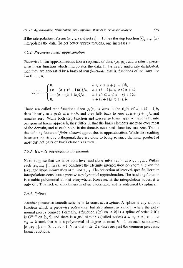
Ch. 12: Approximation, Perturbation, and Projection Methods in Economic Analysis 555
l f the interpolation data are (xi, yi) and ~i(xi) = 1, then the step function ~ i y i ~ i ( x ) interpolates the data. To get better approximations, one increases n.
7.6.2. P iecewise l inear approximation
Piecewise linear approximations take a sequence of data, (x i , Yi), and creates a piece- wise linear function which interpolates ,the data. If the z~ are uniformly distributed, then they are generated by a basis of tent funct ions, that is, functions of the form, for i = O , . . . , n ,
0,
~ i ( x ) = (x - (a + (i - 1 ) h ) ) / h , 1 - (x - (a + i h ) ) / h , O,
a ~< z ~< a + ( i - 1)h, a + (i - 1)h <~ x ~ a + ih, a + ih <~ x <~ a + (i + 1)h, a + ( i + l ) h ~ x ~ b .
These are called tent functions since ~ ( x ) is zero to the right of a + (i - 1)h, rises linearly to a peak at a + ih, and then falls back to zero at a + (i + 1)h, and remains zero. While both step function and piecewise linear approximations fit into our general linear approach, they differ in that the basis elements are zero over most of the domain, and at each point in the domain most basis functions are zero. This is the defining feature of f in i te e lement approaches to approximation. While the resulting bases are not strictly orthogonal, they are close to being so since the inner product of most distinct pairs of basis elements is zero.
7.6.3. Hermi te interpolation polynomials
Next, suppose that we have both level and slope information at xt, • • •, xn. Within each [xi, xi+l] interval, we construct the Hermite interpolation polynomial given the level and slope information at xi and xi+l. The collection of interval-specific Hennite interpolations constitute a piecewise polynomial approximation. The resulting function is a cubic polynomial almost everywhere. However, at the interpolation nodes, it is only C l . This lack of smoothness is often undesirable and is addressed by splines.
7.6.4. Splines
Another piecewise smooth scheme is to construct a spline. A spline is any smooth function which is piecewise polynomial but also almost as smooth where the poly- nomial pieces connect. Formally, a function s ( x ) on [a, b] is a spline of order k if s is C k-2 on [a, b], and there is a grid of points (called nodes) a = xo < x~ < • • - < xn = b such that s is a polynomial of degree at most k - 1 on each subinterval [xi, xi+l], i = 0 , . . . , n - 1. Note that order 2 splines are just the common piecewise linear functions.
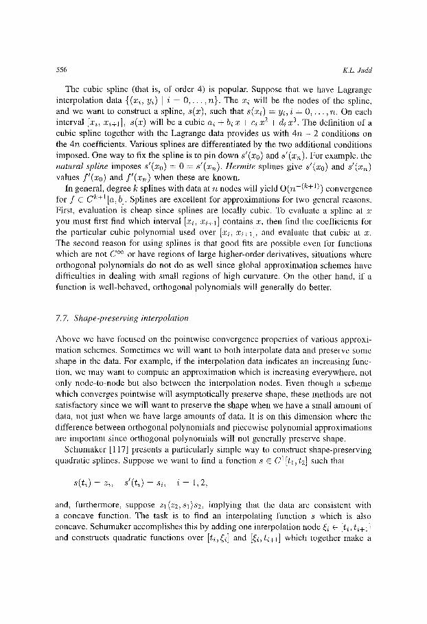
556 K.L. Judd
The cubic spline (that is, of order 4) is popular. Suppose that we have Lagrange interpolation data {(x~, y~) I i = 0 , . . . , n}. The xi will be the nodes of the spline, and we want to construct a spline, s(x), such that s(xi) = Yi, i = 0 , . . . , n. On each interval [xi, xi+l], s(x) will be a cubic a~ + b~ x + e~ x 2 + d~ x 3. The definition of a cubic spline together with the Lagrange data provides us with 4n - 2 conditions on the 4n coefficients. Various splines are differentiated by the two additional conditions imposed. One way to fix the spline is to pin down s'(xo) and s ' (xn) . For example, the natural spline imposes s'(xo) = 0 = s ' (xn) . Hermite splines give s'(xo) and s ' (x~) values f ' ( xo ) and f ' ( x ~ ) when these are known.
In general, degree k splines with data at n nodes will yield O(n - (k+ l ) ) convergence for f c C k+1 [a, b]. Splines are excellent for approximations for two general reasons. First, evaluation is cheap since splines are locally cubic. To evaluate a spline at x you must first find which interval [xi, Xi+l] contains x, then find the coefficients for the particular cubic polynomial used over [xi, xi+1], and evaluate that cubic at x. The second reason for using splines is that good fits are possible even for functions which are not C °~ or have regions of large higher-order derivatives, situations where orthogonal polynomials do not do as well since global approximation schemes have difficulties in dealing with small regions of high curvature. On the other hand, if a function is well-behaved, orthogonal polynomials will generally do better.
7. 7. Shape-preserving interpolation
Above we have focused on the pointwise convergence properties of various approxi- mation schemes. Sometimes we will want to both interpolate data and preserve some shape in the data. For example, if the interpolation data indicates an increasing func- tion, we may want to compute an approximation which is increasing everywhere, not only node-to-node but also between the interpolation nodes. Even though a scheme which converges pointwise will asymptotically preserve shape, these methods are not satisfactory since we will want to preserve the shape when we have a small amount of data, not just when we have large amounts of data. It is on this dimension where the difference between orthogonal polynomials and piecewise polynomial approximations are important since orthogonal polynomials will not generally preserve shape.
Schumaker [117] presents a particularly simple way to construct shape-preserving quadratic splines. Suppose we want to find a function s E C 1 [tl, t2] such that
s(t ) - - s , , i = 1 , 2 ,
and, furthermore, suppose zl(z2, sl)s2, implying that the data are consistent with a concave function. The task is to find an interpolating function s which is also concave. Schumaker accomplishes this by adding one interpolation node ~i E [~i, ~i+1] and constructs quadratic functions over [/.i, ~i] and [~i, ~+l] which together make a
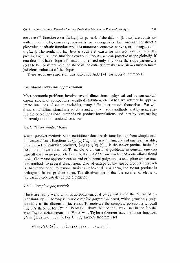
Ch. 12: Approximation, Perturbation, and Projection Methods in Economic Analysis 557
concave C 1 function s on [t~, t~+l]. In general, if the data on [t~, t~+l] are consistent with monotonicity, concavity, convexity, or nonnegativity, then one can construct a piecewise quadratic function which is monotone, concave, convex, or nonnegative on [ti,t~+l]. The nontrivial fact here is such a {i exists for any interpolation data. By piecing together these functions over subintervals, we can preserve shape globally. If one does not have stope information, one need only to choose the slope parameters so as to be consistent with the shape of the data. Schumaker also shows how to make judicious estimates of the slopes.
There are many papers on this topic; see Judd [74] for several references.
7.8. Multidimensional approximation
Most economic problems involve several dimensions - physical and human capital, capital stocks of competitors, wealth distribution, etc. When we attempt to approx- imate functions of several variables, many difficulties present themselves. We will discuss multidimensional interpolation and approximation methods, first by generaliz- ing the one-dimensional methods via product formulations, and then by constructing inherently multidimensional schemes.
7.8.1. Tensor product bases
Tensor product methods build multidimensional basis functions up from simple one- dimensional basis functions. If {qoi(x)}~__ 1 is a basis for functions of one real variable, then the set of pairwise products, {~i(x)~j(y)}~,°°j= 1 is the tensor product basis for functions of two variables. To handle n dimensional problems in general, one can take all the n-wise products to create the n-fold tensor product of a one-dimensional basis. The tensor approach can extend orthogonal polynomials and spline approxima- tion methods to several dimensions. One advantage of the tensor product approach is that if the one-dimensional basis is orthogonal in a norm, the tensor product is orthogonal in the product norm. The disadvantage is that the number of elements increases exponentially in the dimension.
7.8.2. Complete polynomials
There are many ways to form multidimensional bases and avoid the "curse of di- mensionality". One way is to use complete polynomial bases, which grow only poly- nomially as the dimension increases. To motivate the complete polynomials, recall Taylor's theorem for R n in Theorem 1 above. Notice the terms used in the kth de- gree Taylor series expansion. For k = 1, Taylor's theorem uses the linear functions ~f)l ~ {1 ,X t ,X2 , . . . ,Xn}. For h = 2, Taylor's theorem uses
7")2 ~ J~l (J {x21~ . . 2 ~ X n _ l X n } . • ~ X n ~ X l X 2 ~ X l X 3 ~ . . .

558 K.L. Judd
792 contains some cross-product terms, but not all; for example, XlX2X 3 is not in 5o2. In general, the kth degree expansion uses functions in
{ I } g=l
The set 79k is the complete set of polynomials of total degree k. Complete sets of polynomials are often superior to tensor products for multivariate
approximation. The n-fold tensor product of { 1, x , . . . , x k } contains (k+ 1)n elements, far more than 79k. For example, 7)2 contains 1 + n + n(n + 1)/2 elements compa- red to 3 n for the tensor product. Taylor's theorem tells us that many of the tensor product elements add little to the approximation, saying that the elements of 79k will yield a kth order approximation near x °, and but that the n-fold tensor product of {1, x , . . . , x k} can do no better than kth order convergence since it does not contain all degree k + 1 terms. This suggests that a complete family of polynomials will give us nearly as good an approximation as the tensor product of the same order, but with far fewer elements.
7.8.3. Finite element approaches
Finite element methods use bases whose elements have small support. One simple example is bilinear interpolation. Suppose we have the values of f (x , y) at (x, y) = (+ 1, + 1). Then, the following 4 functions form an interpolation basis:
= ¼(1
=
~ 2 ( x , y ) = ¼ ( l ÷ x ) ( 1 - y ) ,
~ 4 ( x , y ) = ¼ ( 1 - x ) ( l ÷ y ) . (46)
The bilinear approximation to f on the square [ -1 , 1] × [ -1 , 1], which is an example of an element, is
f ( - 1 , - 1 ) ¢ l ( x , y ) + f ( 1 , - 1 ) ¢ z ( x , y ) + f ( 1 , 1 ) ¢ 3 ( x , y ) ÷ f ( - 1 , 1 ) ¢ 4 ( x , y ) .
The approximation is linear at each edge, but generally has a saddlepoint curvature on the interior. To interpolate data on a two-dimensional lattice, we create the bilinear approximation on each square.
Finite element methods consist of partitioning a domain into several elements, and patching together the local approximations on the elements, but this is not easy. Since we generally want the result to be a continuous function, care must be taken that resulting approximation is continuous across element boundaries. With bilinear inter- polation, this will hold since any two approximations overlap only at the edges of rectangles, and on those edges the approximation is the linear interpolant between

Ch. 12: Approximation, Perturbation, and Prajection Methods in Economic Analysis 5 5 9
the common vertices. If we know that we are approximating a smooth function, then the kinks at the edges of the elements may make bilinear approximation unappealing. Assuring smoothness at element boundaries is an increasingly difficult problem as we increase the desired degree of differentiability and the dimension. The bilinear finite element scheme is just the simplest of a large number of finite element ap- proximation schemes. There is a large literature on finite element approximations of multidimensional functions (see Burnett [22]).
7.8.4. Neural networks
The previous approximation procedures are based on linear combinations of polyno- mial and trigonometric functions. Neural networks provide us with an alternative and inherently nonlinear functional form for approximation. A single-layer neural network is a function of the form
F(x;/3) -2 h ~9 xi (47)
where x E R n is the vector of inputs and h and g are scalar functions. A common form chooses 9(x) = x, reducing (47) to the form h(t3Tx). A single hidden-layer feedforward network is the form
F(x; /3 ,7) ~ 7jl~, g xi • \ i = 1 ~ /
(48)
Note the simplicity of the functional forms; this simplicity makes neural network approximations easy to evaluate.
The data for a neural network consists of (yj, xJ) pairs such that yj C R is supposed to be the output of a neural network if xJ E R n is the input. This requirement imposes conditions on the parameters/3 in (47) and/3 and 3/in (48). One fits single-layer neural networks by finding fl to solve
rain E ( y j - F(xJ;f l)) 2 J
and the objective of a single hidden-layer feedforward network is to solve
min E ( y j - F(xJ;p , 3')) 2, /3,q,
J
which are just instances of nonlinear least squares fitting.

560 K.L. Judd
The approximating power of neural network approximation is indicated by theorems of Horni, Stinchcombe and White (see White [122] for a wide-ranging discussion of neural networks and their properties). Let G be a continuous function, G : R -+ R, such that f~-~oo G(x ) dx is finite and nonzero and G is L p for 1 ~< p < ec. Let
+ b j) , b j,/3j C R, L j = l
w j C R n, w j ¢ 0 , m = 1 , 2 , . . . }
be the set of all possible single-hidden layer feedforward neural networks using G as the hidden layer activation function.
THEOREM 11. Let f : R ~ -+ R be continuous. Then f o r all e > O probability measure #, and compact sets K C R ~, there is a 9 E z ,n (G) such that
sup I f (z) - g ( z ) l < xEK
and
L If(x) - g(x)[ d/z < e.
This also holds when G is a squashing functions, i.e., G : R --+ [0, 1], G is nonde- creasing, lim:~-+oo G(x) = 1, and l imx~-oo G(x ) = 0.14
These are universal approximation results which justify the use of neural network approximation, and help explain its success. There is some evidence that neural net- work approximation methods may be particularly efficient at, multidimensional ap- proximation in the sense of needing relatively few free parameters; see Barton [6] for a recent result. The theoretical development of neural networks is proceeding, but is inherently difficult because of the nonlinearity of this approach.
8. Applications of approximation to dynamic programming
Approximation methods are a key part of most numerical procedures. They are par- ticularly important in discrete-time dynamic programming problems. These problems
14Note that a squashing function is a cumulative distribution function and vice-versa. A coimnon choice for G is the sigmoid function, G(x) = 1/(1 + e-X).

Ch. 12: Approximation, Perturbation, and Projection Methods in Economic Analysis 561
are among the most useful and basic of dynamic economic problems, with well- understood theoretical properties. We will briefly discuss them and the approximation aspects of numerical dynamic programming.
Let 7r(u, x)be profit flow if the state is x and the control is u. Suppose the law of motion is
z~+l =g(xt, ~t).
Then the value function, V(x), solves
V(x) = maxTr(u, x) + flV(g(x, u) ) - (TV)(x). (49)
The standard theoretical procedure is to iterate on the basic functional equation, (49). If we could handle arbitrary functions, we would start with a guess, V0, and then compute the sequence {Vn} generated by
v~ - TEn-1 . (50)
This procedure converges when viewed as a mapping in the space of value functions. On the computer, however, one cannot store arbitrary functions. There are several
details which need to be decided to compute approximations to (50). Since we cannot deal directly with the space of continuous functions, we focus on a finite-dimensional subspace. We will approximate V(x) as a finite linear sum of basis functions.
N
i = l
(51)
Numerical procedures construct a V(x) which approximately satisfies the Bellman equation, (49). More specifically, the objective is to find a vector, ~ E R N, such that V solves (49) as closely as possible.
The basic task is to replace T, an operator mapping continuous functions to con- tinuous functions, with a finite-dimensional approximation, 2r, which maps functions of the form in (51) to functions of the same form. We construct 2~ in two steps. First, we choose a finite collection, X, of points x, and evaluate (T~')(z) at x C X. We will refer to this as the maximization step since it is the maximization problem in (49) at x. The resulting values are points on the function TV. Since we are approximating a continuous value function, we use that information to choose a value function of form (51) which "best" summarizes the information generatedconcerning TV. This is the critical approxima~on step, and we denote the result TV. In essence, T takes a function of form (51), V, and maps it to another function of the same form, and is therefore a mapping in the space of the ~ coefficients, and the objective is to find a

562 K.L. Judd
fixed point for T in the space of coefficients. We can also view T as a mapping from continuous functions to the finite-dimensional subspace representable as V ( x , ~), in
which case the problem is to find a fixed point of T in the space of functions of form
(51). The details of the approximation aspects of this procedure - choosing a basis for
the expression of V, choosing points X to evaluate T V , and fitting the data - are important. We next discuss some basic approaches.
8.1. Discretization methods
The simplest approximation procedure is to discretize the state space, that is, they re- place the problem on a continuous state space with one with a finite number of points. This has the advantage of reducing the problem to one of finite matrices. The other advantage is that the resulting analysis exactly solves some similar economic problem. See Rust [112] for a discussion of numerical dynamic programming procedures. Even in the case of discrete-state dynamic programming, projection solution ideas come into use. The key computation in the discrete-state approach is the solution of a large linear system. This can be accomplished approximately by using the GMRES method (see Saad and Schulz [113]) which essentially computes a few directions and finds an approximate solution which is spanned by these directions and minimizes a loss function.
While the discretization method does not obviously fit the description above, it is generally equivalent to approximating the value function with a step function. 15
However, step functions are highly inefficient ways to approximate a smooth value function. Because of this, the discretized state space method is unlikely to be of much value in economic analysis outside of naturally discrete problems, one-dimensional problems, or problems where the solutions are so nonsmooth that discretization is competitive with smooth approximation schemes. The impracticality of discretization is indicated by the fact that supercomputers are often used. Multidimensional problems are practically impossible, even for supercomputers, since the "curse of dimensionali- ty" is particularly vexing for this method; if N points are used for a one-dimensional problem, then N a points will be used for a d -dimensional problem. There are several ingenious methods for making discrete state problems more efficient; see Rust [112] for a description of these algorithms. We will focus on the alternatives presented by the application of approximation ideas.
15After computing the solution to (50), many users then use linear interpolation to estimate the value function at points not part of the discretized state space. Since this linear interpolation is done only after the value iteration is completed, it does not affect these comments and it's contribution to improving the algorithm's accuracy is limited.
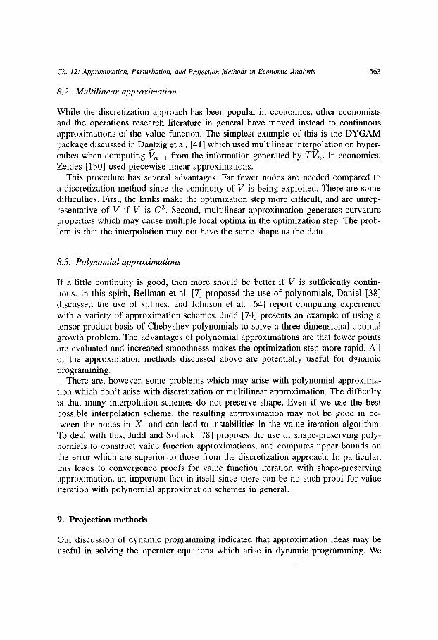
Ch. 12: Approximation, Perturbation, and Projection Methods in Economic Analysis 563
8.2. Multil inear approximation
While the discretization approach has been popular in economics, other economists and the operations research literature in general have moved instead to continuous approximations of the value function. The simplest example of this is the DYGAM package discussed in Dantzig et al. [41 ] which used multilinear interpolation on hyper- cubes when computing Vn+l from the information generated by TV~. In economics, Zeldes [130] used piecewise linear approximations.
This procedure has several advantages. Far fewer nodes are needed compared to a discretization method since the continuity of V is being exploited. There are some difficulties. First, the kinks make the optimization step more difficult, and are unrep- resentative of V if V is C 2. Second, multilinear approximation generates curvature properties which may cause multiple local optima in the optimization step. The prob- lem is that the interpolation may not have the same shape as the data.
8.3. Polynomial approximations
If a little continuity is good, then more should be better if V is sufficiently contin- uous. In this spirit, Bellman et al. [7] proposed the use of polynomials, Daniel [38] discussed the use of splines, and Johnson et al. [64] report computing experience with a variety of approximation schemes. Judd [74] presents an example of using a tensor-product basis of Chebyshev polynomials to solve a three-dimensional optimal growth problem. The advantages of polynomial approximations are that fewer points are evaluated and increased smoothness makes the optimization step more rapid. All of the approximation methods discussed above are potentially useful for dynamic programming.
There are, however, some problems which may arise with polynomial approxima- tion which don't arise with discretizafion or multilinear approximation. The difficulty is that many interpolation schemes do not preserve shape. Even if we use the best possible interpolation scheme, the resulting approximation may not be good in be- tween the nodes in X, and can lead to instabilities in the value iteration algorithm. To deal with this, Judd and Solnick [78] proposes the use of shape-preserving poly- nomials to construct value function approximations, and computes upper bounds on the error which are superior, to those from the discretization approach. In particular, this leads to convergence proofs for value function iteration with shape-preserving approximation, an important fact in itself since there can be no such proof for value iteration with polynomial approximation schemes in general.
9. Projection methods
Our discussion of dynamic programming indicated that approximation ideas may be useful in solving the operator equations which arise in dynamic programming. We
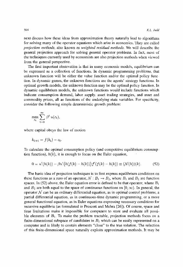
564 K.L. dudd
next discuss how these ideas from approximation theory naturally lead to algorithms for solving many of the operator equations which arise in economics. They are called p r o j e c t i o n me thods , also known as w e i g h t e d res idua l me thods . We will describe the general projection approach for solving general operator problems. In fact, most of the techniques currently used by economists are also projection methods when viewed from the general perspective.
The first important observation is that in many economic models, equilibrium can be expressed as a collection of functions. In dynamic programming problems, that unknown function will be either the value function and/or the optimal policy func- tion. In dynamic games, the unknown functions are the agents' strategy functions. In optimal growth models, the unknown function may be the optimal policy function. In dynamic equilibrium models, the unknown functions would include functions which indicate consumption demand, labor supply, asset trading strategies, and asset and commodity prices, all as functions of the underlying state variables. For specificity, consider the following simple deterministic growth problem:
O¢3
max Ct
t=O
where capital obeys the law of motion
kt+l = f ( k t ) - ct .
To calculate the optimal consumption policy (and competitive equilibrium consump- tion function), h ( k ) , it is enough to focus on the Euler equation,
0 = u ' ( h ( k ) ) - f l u ' ( h ( f ( k ) - h ( k ) ) ) f ' ( f ( k ) - h ( h ) ) =_ (Af(h))(k). (52)
The basic idea of projection techniques is to first express equilibrium conditions on these functions as a zero of an operator, .M : B1 --+ B2, where B 1 and/32 are function spaces. In (52) above, the Euler equation error is defined to be that operator, where B1 and B2 are both equal to the space of continuous functions on [0, oc). In general, the operator N" can be an ordinary differential equation, as in optimal control problems, a partial differential equation, as in continuous-time dynamic programming, or a more general functional equation, as in Euler equations expressing necessary conditions for recursive equilibria (as formulated in Prescott and Mehra [26]). Of course, space and time limitations make it impossible for computers to store and evaluate all possi- ble elements of B1. To make the problem tractable, projection methods focus on a finite-dimensional subspace of candidates in B1 which can be easily represented on a computer and is likely to contain elements "close" to the true solution. The selection of this finite-dimensional space naturally exploits approximation methods. It may be

Ch. 12: Approximation, Perturbation, and Projection Methods in Economic Analysis 565
difficult for the computer to evaluate N , in which case we find a computable oper- ator, J~, which is "similar" to N'. Within the finite-dimensional space of candidate solutions, we find an element which is "almost" a zero of ~ ' .
While the basic idea is natural, there are many details. The key details are specifying the approximation method we will use, the finite-dimensional subspace within which we look for an approximate solution, and the computer representation of N', defining what "close" and "almost" mean, and finding the approximate solution. By studying these details, we will see how to implement these ideas efficiently to solve numerically interesting dynamic nonlinear economic problems.
9.1. General projection algorithm
We next describe the projection method in a general context. One begins with an operator equation representation of the problem, that is, one reduces the economic problem to finding an operator iV" and a function f such that equilibrium is represented by the solution to
A/" ( f ) = 0
where f : D C R N --+ R M, N" : B1 -+ B2, and the Bi are function spaces. Typically 34* is a composition of algebraic operations, differential and integral operators, and functional compositions, and is frequently nonlinear. We shall show how to implement the canonical projection technique in a step-by-step fashion. We first give an overview of the approach, then highlight the critical issues for each step, and discuss how the steps interact.
The first step is to decide how to represent approximate solutions. One general way is to assume that our approximation, f , is built up as a linear combination of simple functions. We will also need a concept of when two functions are close. Therefore, the first step is to choose a basis and an appropriate concept of distance:
Step 1. Choose bases, ~bj = {(~:~i}~?°l , and inner products, (., .)j, over Bj , j = 1,2.
The basis over B1 should be flexible, capable of yielding a good approximation for the solution, and the inner products should induce useful norms on the spaces.
Next, we decide how many basis elements to use and how to implement iV:
Step 2. Choose a degree of approximation r~ for f , a computable approximation N" of iV", and a collection of n functions from B2, p~ : D --+ /~M, i = l , . . . , ~r~,.
The approximate solution will be f -- 2in.=1 aicpi(:c). The convention is that the ~i increase in "complexity" and "nonlinearity" as i increases, and that the first n elements are used. The best choice of n cannot be determined a priori. Generally,
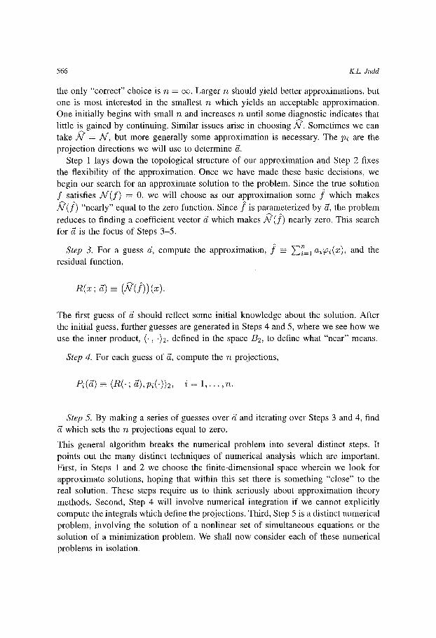
566 K.L Judd
the only "correct" choice is n = ec. Larger n should yield better approximations, but one is most interested in the smallest n which yields an acceptable approximation. One initially begins with small n and increases n until some diagnostic indicates that little is gained by continuing. Similar issues arise in choosing .~. Sometimes we can take .~ = N', but more generally some approximation is necessary. The Pi are the projection directions we will use to determine &
Step 1 lays down the topological structure of our approximation and Step 2 fixes the flexibility of the approximation. Once we have made these basic decisions, we begin our search for an approximate solution to the problem. Since the true solution f satisfies N ' ( f ) = 0, we will choose as our approximation some f which makes
2~(f) "nearly" equal to the zero function. Since f is parameterized by 6, the problem
reduces to finding a coefficient vector d which makes .~ ( f ) nearly zero. This search for 6 is the focus of Steps 3-5.
Step 3. For a guess & compute the approximation, f _= ~i"- , ai~.i(x), and the residual function,
R ( x ; -
The first guess of d should reflect some initial knowledge about the solution. After the initial guess, further guesses are generated in Steps 4 and 5, where we see how we use the inner product, (., ")2, defined in the space 132, to define what "near" means.
Step 4. For each guess of & compute the n projections,
- ( R ( . ; i = l , . . . , , J .
Step 5. By making a series of guesses over ff and iterating over Steps 3 and 4, find which sets the n projections equal to zero.
This general algorithm breaks the numerical problem into several distinct steps. It points out the many distinct techniques of numerical analysis which are important. First, in Steps 1 and 2 we choose the finite-dimensional space wherein we look for approximate solutions, hoping that within this set there is something "close" to the real solution. These steps require us to think seriously about approximation theory methods. Second, Step 4 will involve numerical integration if we cannot explicitly compute the integrals which define the projections. Third, Step 5 is a distinct numerical problem, involving the solution of a nonlinear set of simultaneous equations or the solution of a minimization problem. We shall now consider each of these numerical problems in isolation.
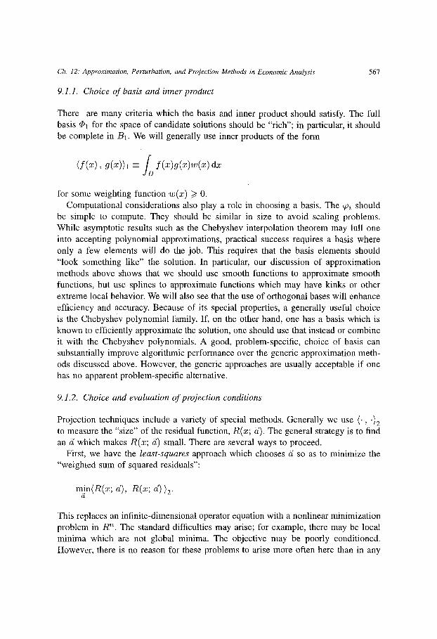
Ch. 12: Approximation, Perturbation, and Projection Methods in Economic Analysis
9.1.1. Choice of basis and inner product
567
There are many criteria which the basis and inner product should satisfy. The full basis ~1 for the space of candidate solutions should be "rich"; in particular, it should be complete in/3i. We will generally use inner products of the form
( f ( x ) , g(x))~ =_/D f(x)g(x)w(x)dx
for some weighting function w(x) >> O. Computational considerations also play a role in choosing a basis. The ~ should
be simple to compute. They should be similar in size to avoid scaling problems. While asymptotic results such as the Chebyshev interpolation theorem may lull one into accepting polynomial approximations, practical success requires a basis where only a few elements will do the job. This requires that the basis elements should "look something like" the solution. In particular, our discussion of approximation methods above shows that we should use smooth functions to approximate smooth functions, but use splines to approximate functions which may have kinks or other extreme local behavior. We will also see that the use of orthogonal bases will enhance efficiency and accuracy. Because of its special properties, a generally useful choice is the Chebyshev polynomial family. If, on the other hand, one has a basis which is known to efficiently approximate the solution, one should use that instead or combine it with the Chebyshev polynomials. A good, problem-specific, choice of basis can substantially improve algorithmic performance over the generic approximation meth- ods discussed above. However, the generic approaches are usually acceptable if one has no apparent problem-specific alternative.
9.1.2. Choice and evaluation of projection conditions
Projection techniques include a variety of special methods. Generally we use (-, ')2 to measure the "size" of the residual function, R(x; g). The general strategy is to find an ~ which makes R(x; if) small. There are several ways to proceed.
First, we have the least-squares approach which chooses d so as to minimize the "weighted sum of squared residuals":
rn~n</~(x; d), R(x; d)>2"
This replaces an infinite-dimensional operator equation with a nonlinear minimization problem in R "~. The standard difficulties may arise; for example, there may be local minima which are not global minima. The objective may be poorly conditioned. However, there is no reason for these problems to arise more often here than in any

568 K.L. Judd
other context, such as maximum likelihood estimation, where optimization problems are solved numerically.
While the least-squares method is a direct approach to making R(x; d) small, most projection techniques find approximations by fixing n projections and choosing d to make the projection of the residual function in each of those n directions zero. Formally, these methods find ~7 such that (R(x; d), pi(x))2 = 0 for some specified collection of functions, Pi. Different choices of the Pi defines different implementa- tions of the projection method.
One such technique is the Galerkin method. In the Galerkin method we use the first n elements of the basis for the projection directions. Therefore, g is chosen to solve the equations:
_= (R(z; = o , i =
Notice that here we have reduced the problem of solving a functional equation to solving a finite set of finite-dimensional nonlinear equations. In some cases in physics, the Galerkin projection equations are the first-order conditions to some least-squares minimization problem, in which case the Galerkin method is also called the Rayleigh- Ritz method. This is not as likely to happen in economics problems because of the inherent nonlinearities.
There are obviously many ways to implement the projection idea. A collocation X" method takes n points from the domain D, { ~}i=1, and chooses g to solve
R(x i ; 6) =0, i = 1 , . . . , n .
This is a special case of the projection approach since R(xi; 6) equals the projection of R(x; d) against the Dirac delta function at x~, (R(x; if), 5(x - xi))2. Orthogonal collocation chooses the collocation points in a special way. The chosen xi are the zeros of the n ' th basis element, where the basis elements are orthogonal with respect to the inner product. The Chebyshev interpolation theorem suggests its power. Suppose D = [ - 1 , 1] and we have found an d such that R(z~ ; 6) = O, i = 1, . . . , n, where the z~ ~ are the n zeros of Tn. As long as R(x; 6) is smooth in x, the Chebyshev interpolation theorem says that these zero conditions force R(x; 6) to be close to zero for all x, and that these are the best possible points to use if we are to force R(x; 6) to be close to zero. It is not certain that even orthogonal collocation is a reliable method; fortunately, its performance turns out to be surprisingly good.
Choosing the projection conditions is a critical decision since the major computa- tional task is the computation of those projections. The collocation method is fastest in this regard since it only uses the value of _R at n points. More generally, the pro- jections will involve integration. In some cases one may be able to explicitly perform the integration. This is generally possible for linear problems, and possible for special nonlinear problems. However, our experience is that this will generally be impossible
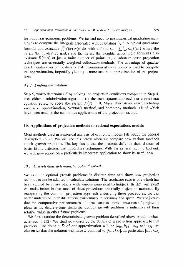
Ch. 12: Approximation, Perturbation, and Projection Methods in Economic Analysis 569
for nonlinear economic problems. We instead need to use numerical quadrature tech- niques to compute the integrals associated with evaluating (., .). A typical quadrature
formula approximates f : f ( x ) w ( x ) d x with a finite sum 2 i n 1 w i f ( z i ) where the xi are the quadrature nodes and the wi are the weights. Since these formulas also evaluate R(x; d) at just a finite number of points, xi, quadrature-based projection techniques are essentially weighted collocation methods. The advantage of quadra- ture formulas over collocation is that information at more points is used to compute the approximation, hopefully yielding a more accurate approximation of the projec- tions.
9.1.3. Finding the solution
Step 5, which determines 6 by solving the projection conditions computed in Step 4, uses either a minimization algorithm (in the least-squares approach) or a nonlinear equation solver to solve the system P(6) = 0. Many alternatives exist, including successive approximation, Newton's method, and homotopy methods, all of which have been used in the economics applications of the projection method.
10. Applications of projection methods to rational expectations models
Most methods used in numerical analysis of economic models fall within the general description above. We will see this below when we compare how various methods attack growth problems. The key fact is that the methods differ in their choices of basis, fitting criterion, and quadrature techniques. With the general method laid out, we will now report on a particularly important application to show its usefulness.
]O.l. Discrete-time deterministic optimal growth
We examine optimal growth problems in discrete time and show how projection techniques can be adapted to calculate solutions. The stochastic case is one which has been studied by many others with various numerical techniques. In fact, one point we make below is that most of these procedures are really projection methods. By recognizing the common projection approach underlying these procedures, we can better understand their differences, particularly in accuracy and speed. We conjecture that the comparative performances of these various implementations of projection ideas in the discrete-time stochastic optimal growth problem is indicative of their relative value in other future problems.
We first examine the deterministic growth problem described above which is char- acterized in (52). We shall now describe the details of a projection approach to that problem. The domain D of our approximation will be [km, kM]. km and kM are chosen so that the solution will have k confined to [k~, kM]. In particular, [k~, kM]

570 K.L. Judd
must contain the steady state, a point which we can determine before calculations begin. Our approximation to h is parametrically given by
n
i = 1
where n is the number of terms used. Common choices include the Chebyshev poly- nomials ¢~(k) ~ T~-i (2(k - km) / (kM - kin) - 1), the tent functions, or the ordinary polynomials.
In this problem, N" is a s impleoperator using only arithmetic operations and com- position. Therefore, we can take N" = N'. Since h is continuous, we define .Af to have domain and range in C°[k,~, kM]. Hence, B1 = B2 = C°[km, kM], the continuity of N" in the L ~ norm following from the u, f , and/z being C 1 in all their arguments. Given the Euler equation (52), the residual function becomes
R ( k ;6) = u ' (h(k ; 6)) - flu' (h ( f ( k ) - h(k ; 6); 6 ) ) f ' ( f ( k ) - h(k ; 6))
=N(h). To compute & we can do one of several things. First, we consider orthogonal
collocation. We choose n values of k, denoted by ki, i = 1 , . . . , n. We then choose 6 so that R(ki; 6) = 0 for each i. Orthogonal collocation chooses the ki to be the n zeros of ~b. The Chebyshev interpolation theorem strongly argues for using Chebyshev polynomials in this case. I f R(ki; 6) = 0 for each ki, then we would like to conclude that R(ki; 6) is the zero function on the domain D. The Chebyshev interpolation theorem says that this is most justified if the ki were the Chebyshev zeros, and that if we use Chebyshev zeros, R(k; ~) will likely be nearly zero.
We could also implement the Galerkin method. If we use Chebyshev polynomials as a basis, then we use projections with the inner product
~k kM ( f ( k ) , g(k)) =- f ( k )g (k )w(k ) dk
where
__± 1/2) 2
With this choice of inner product, the basis is orthogonal. The Galerkin method computes the n projections
f k kM P i ( a ) = R ( k ; 6 ) ¢ i ( k ) w ( k ) d k , i = l , . . . , n , m
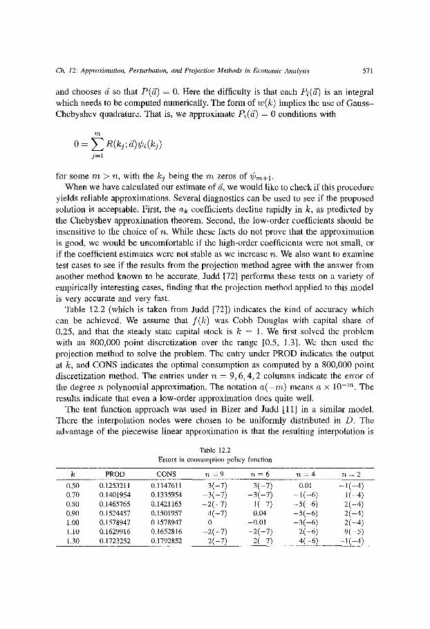
Ch. 12: Approximation, Perturbation, and Projection Methods in Economic Analysis 571
and chooses d so that P(d) = O. Here the difficulty is that each P~(d) is an integral which needs to be computed numerically. The form of w ( k ) implies the use of Gauss- Chebyshev quadrature. That is, we approximate Pi (~) = 0 conditions with
o = R ( k j ; j = l
for some ra > n, with the kj being the m zeros of ~b~+l. When we have calculated our estimate of ~, we would like to check if this procedure
yields reliable approximations. Several diagnostics can be used to see if the proposed solution is acceptable. First, the ak coefficients decline rapidly in k, as predicted by the Chebyshev approximation theorem. Second, the low-order coefficients should be insensitive to the choice of n. While these facts do not prove that the approximation is good, we would be uncomfortable if the high-order coefficients were not small, or if the coefficient estimates were not stable as we increase n. We also want to examine test cases to see if the results from the projection method agree with the answer from another method known to be accurate. Judd [72] performs these tests on a variety of empirically interesting cases, finding that the projection method applied to this model is very accurate and very fast.
Table 12.2 (which is taken from Judd [72]) indicates the kind of accuracy which can be achieved. We assume that f ( k ) was Cobb-Douglas with capital share of 0.25, and that the steady state capital stock is k = 1. We first solved the problem with an 800,000 point discretization over the range [0.5, 1.3]. We then used the projection method to solve the problem. The entry under PROD indicates the output at k, and CONS indicates the optimal consumption as computed by a 800,000 point discretization method. The entries under n = 9, 6, 4, 2 columns indicate the error of the degree n polynomial approximation. The notation a ( - m ) means a x 10 - ~ . The results indicate that even a low-order approximation does quite well.
The tent function approach was used in Bizer and Judd [11] in a similar model. There the interpolation nodes were chosen to be uniformly distributed in D. The advantage of the piecewise linear approximation is that the resulting interpolation is
Table 12.2 Errors in consumption policy function
k PROD CONS n = 9 n = 6 n = 4 n = 2
0.50 0.1253211 0.1147611 3(-7) 3(--7) 0.01 -1( -4) 0 .70 0.1401954 0.1335954 -3( -7) -3 ( -7 ) -1 ( -6) 1(--4) 0 .80 0.1465765 0.1421165 -2( -7) -1(--7) --5(-6) 2(-4) 0 .90 0.1524457 0.1501957 4(-7) 0.04 -5( -6) 2(-4) 1.00 0.1578947 0.1578947 0 -0.01 -3( -6) 2(-4) 1.10 0.1629916 0.1652816 --2(-7) -2 ( -7) 2(-6) 9(-5) 1.30 0.1723252 0.1792852 2(-7) 2(-7) 4(-6) --1(--4)
572 K.L. Judd
shape-preserving. This may be useful since we know that h is monotone increas- ing. However, the shape-preservation considerations turn out not to be important relative to the differentiability considerations which argue for Chebyshev polynomi- als. The policy functions computed in Judd [72] using Chebyshev polynomials were monotone increasing, and using tent functions substantially reduced the algorithm's efficiency.
10.2. Stochastic optimal growth
We next turn to a stochastic optimal growth model. This example will show us how to handle multidimensional problems and the conditional expectations which arise in stochastic dynamic problems. We will also be able to describe the parameterized expectations method of solving rational expectations models.
More specifically, we examine the problem
k t + l = Ot f ( ] c t ) -- e t ,
ln0t+l = plnOt + :t+~ (53)
where Ot is a stationary AR(1) multiplicative productivity parameter. We will assume that the productivity shocks et "- N(0, o -2) are independent. In this problem, both the beginning-of-period capital stock and the current value of 0 are needed for a sufficient description of the state. Hence, consumption is a function of both k and 0, h(h, 0), and the Euler equation is
u/(h(k,O)) = /3E{u/(h(Of(h)-h(k,O),O) )Of'(Of(k)-h(k,O)) I O }. (54)
At this point, we will rewrite the Euler equation to make it more linear. We know that projection algorithms work well for linear problems. Perhaps our algorithm will do better if we make it more like a linear problem. To that end, rewrite (54) as
0 = h(k, 0)
Note that (55) has two terms, one linear in h(k, 0), and the other is similar to a CRTS function of next period's potential consumption values. Similar stochastic growth problems were investigated in Judd [72] and in the Taylor-Uhlig [120] symposium. We shall now describe and compare the various methods.
Ch. 12: Approximation, Perturbation, and Projection Methods in Economic Analysis 573
The procedure for finding h is similar to the deterministic case. First of all, we need to approximate the policy function. Judd [72] and Coleman [36] use approximations of the form
n k 7~,0
h(k, O; a) = ~ ~ aij¢ij(k O) i = l j = l
where the ~/Jij functions are Chebyshev functions of k and 0 in Judd, and tent func- tions of Ink and log 0 in Coleman [36]. Judd also considered complete polynomials. Comparisons followed the considerations outlined above. Since the policy function is smooth, the smooth approximation procedures did better with the complete poly- nomial approach doing best, that is, the greatest accuracy per unit of computer time. Coleman's choice of a finite element approach reduced efficiency since it used far more basis elements; furthermore, it cannot switch to a complete polynomial ap- proach. These differences between the spectral approach advocated in Judd and the finite element approach used in Coleman become even larger as we move to higher dimensions.
In their approach to the stochastic growth model, Den Haan and Marcet [57] pa- rameterized the policy function to be
h(k, O) = (k62053e 61)l/'y = (exp{Sl + 52 in k + 53 In 0}) I/'Y (56)
that is, they assume that log consumption is a linear function of In k and log 0. However, this basis is not orthogonal. When they tried to improve the approximation to a quadratic form in In k and log0, the lack of orthogonality lead to difficulties which prevented them from improving on the linear approximation. They argue that the collinearity of their basis elements is "a fortunate situation" and justifies their focus on low-order polynomial approximations. In contrast, the use of orthogonal bases in Judd and the use of a finite element approach in Coleman leads to no difficulties in finding substantially better approximations beyond low-order polynomials.
The comparisons of the Coleman, Den Haan and Marcet, and Judd approaches to solving (54) illustrates the importance of approximation ideas. Den Haan and Marcet, and Judd use polynomials to approximate what is presumed to be a smooth function. Coleman's contrasting use of finite elements introduces kinks in the approximation which forces him to use many elements. The finite element approach and the or- thogonal polynomial approach avoids the multicollinearity problems which limited Den Haan and Marcet to low-order approximations. As these papers discuss, these differences lead to considerable differences in computational speed and accuracy in the final result.
574 K.L. Judd
10.3. Problems with inequality constraints
The optimal growth problem described above was simple in that the equilibrium was described in terms of an Euler equation which always had an interior solution. In some problems, constraints mean that the first-order conditions must be complemented with complementary slackness conditions. This was the nature of the problems which were the first to lead to numerical solutions of nonlinear rational expectations equilibria. Gustafson [56] investigated the problem of equilibrium storage of a storable commod- ity. He assumed that output in period t is an exogenous random variable, Yt, which is divided between a change in storage, St+l - S t (cot is the beginning-of-period-t stock), and consumption, ct. In equilibrium, price is a function of total stock, p(St + zt), and obeys the conditions
p(s~ + x~) - E{p(S~+l + x~+~)}/> 0,
(p(St + xt) -- E{p(St+I -t- xt+l) })St+l = 0 (57)
where St+l = St + xt - D(p(St + xt)) and D(p) is the demand function. In some states of the world, the equilibrium storage level will be zero and the price
function will not be a smooth. Gustafson [56] used a piecewise linear approximation of the equilibrium price function in his solution method. Piecewise linear approxi- mations are relatively inefficient because many pieces are necessary to get a good approximation. In their analysis of the problem (which also generalized Gustafson to handle endogenous output) Williams and Wright solved for E{pt+l [ St+l } as a func- tion of St+l, expressing this year's expectation of next year's price conditional on the amount stored for next year. This function determines the current price, future supply, and current stockpiling through an Euler equation similar to (57), but is smooth be- cause it is a conditional expectation. Hence, they found that a low-order polynomial approximation was sufficient to solve the problem. Miranda and Helmburger [98] also used this insight in their analysis of stockpiling. Christiano and Fisher [32] applied the Wright-Williams technique for handling the inequality constraint to a constrained version of (53) and found similar advantages to using a smooth approximation.
This discussion points out two facts when dealing with inequality constraints. First, we can still use the same approximation ideas but we may have to adapt to handle the kinks which may arise. Second, skillful construction of the problem may result in finding a smooth function which characterizes equilibrium and allows us to use the more efficient smooth approximation schemes. Again, approximation ideas can be exploited to produce superior methods.
10.4. Dynamic games
Methods which are useful for dynamic programming are also naturally natural for computing closed-loop (also known as Markov) equilibria of dynamic games. This
Ch. 12: Approximation, Perturbation, and Projection Methods in Economic Analysis 575
holds since each player solves a dynamic programming problem, and equilibrium can be expressed as a coupled collection of Bellman equations for each player's dynamic programming problem. Kotlikoff, Shoven and Spivak [80] used ordinary polynomials in their study of strategic saving and bequests. Miranda and Rui [99] computed closed-loop equilibria for dynamic stockpiling games among commodity producing countries. They used Chebyshev polynomial approximations to players' value functions and projection methods to determine equilibrium value functions. In both cases, equilibrium was computed with relative ease.
10.5. Continuous time problems
The examples above have been of discrete-time systems. Projection methods have also been used to solve continuous-time models. One simple example is the canonical continuous-time optimal growth problem described above in (21), which reduced to solving the differential equation:
o : C ' ( k ) ( f ( k ) - C ( k ) ) u " ( C ( k ) ) (p - f ' ( k ) ) - E(k; C) .
Judd [71] used a basis of Chebyshev polynomials to approximate C(k) with C(k, a) = En- on i=0 ai a large interval of capital stocks. Again, the performance of the algorithm was very good, independent of the details of the implementation. In fact, it easily outperformed the more commonly used shooting approach to the problem. Judd also extended this model to allow for taxation and uncertainty in continuous time. In all cases, accurate results were obtained quickly. Since projection methods were initially developed to deal with continuous-time systems represented by ordinary and partial differential equations, this is not surprising. One suspects that continuous-time systems in general will be readily computed with projection methods.
10.6. Models with asymmetric information
Many of the examples discussed above reduced to applying the projection method to standard mathematical problems - ordinary and partial differential equations and integral equations. To demonstrate the flexibility of the projection method, we next examine a very different kind of problem - equilibrium where individual agents have different information. These problems do not reduce to any of the standard operator problems discussed in applied mathematical literature. However, one can attack them successfully with the projection method. We will first describe an application to asset markets with asymmetric information. We will then discuss other economic problems where these methods have potential.
576 K.L. Judd
10.6.1. Information and asset markets'
Asset market equilibrium with imperfect information have been rigorously studied in recent years. Grossman [54] and Grossman and Stiglitz [55] began a long literature on the partial equilibrium analysis of security markets with asymmetric information. However, much of this literature makes very special and simple assumptions about the distribution of returns, the information asymmetries, investor tastes, and asset structure. The restrictions substantially limit the generality of the results and the range of questions which can be addressed.
Recently, Judd and Bernardo [76] applied projection methods to analyze these models without special functional form assumptions. A simple one-period investment problem illustrates the method. Suppose each investor invests in two assets. The safe asset pays out R dollars per dollar invested, and the basic risky asset (we will call it stock) pays out Z dollars per share. If an investor begins the first period with W dollars in cash and coo shares of stock, and ends the first period with co shares of stock which trade at a price of p dollars per share, his second, and final, period consumption will be
= ( w - (co - coo)p) R + c o 2 . (58)
The first-order condition for the choice of co will be
0 : E { u ' ( ~ ) ( 2 - pR) 1 I} (59)
where I is the investor's information set.
10.6.2. Computing conditional expectations
The conditional expectation in (59) implies that our equilibrium concept involves a conditional expectation. Numerical implementation of the conditional expectation conditions is the most challenging aspect of this problem. To solve this problem, Judd and Bernardo used the following definition of conditional expectation:
Z(X) = E{YIX }
if and only if
E{(Z(X) - Y)f(X)} : 0
for all bounded measurable functions, f ( X ) , of X. Intuitively, this says that the predic- tion error of the conditional expectation, E { Y [ X}, is uncorrelated with any measur- able function of the conditioning information, X. This definition replaces the condi- tional expectation with an infinite number of unconditional expectation conditions.

Ch. 12: Approximation, Perturbation, and Projection Methods in Economic Analysis 577
10.6.3. Computing an asymmetric inJbrmation rational expectations equilibrium
We now show how to compute an equilibrium. Assume three types of investors, with type i investors observing Yi. The state of the market includes all private signals, g = (Yl, Yz, Y3), but each investor sees only the market-clearing price and his own information. Therefore, a rational expectations equilibrium includes a price function p(y) and type-specific demand policy functions, Oi(p, Yi) for i = 1,2, 3, such that
given p(y), O~ solves (59) for i = 1,2,3, and ~=10 . i (y i , p (y ) ) : 1 for all states y, where total supply is 1.
In their solution, Judd and Bernardo [76] approximate the price law, P(yl, Y2, Y3), and the demand rules, Oi(p(y), Yi), with multivariate polynomials. To determine the unknown coefficients in those polynomials, they impose projection conditions on the investors' first-order conditions. The first-order-condition for a type i investor
Ey , z{u ' (S i ) (Z -pR) lyi,p } = 0 , i = 1,2,3. (60)
Using the definition of conditional expectation given above they impose projection conditions of the form
Ey,z - p(y)R)p(v/ } : o, (61)
for various choices of j , k >~ 0. The condition in (61) states that the prOduct of the excess return and the marginal utility of consumption for a type i agent is uncorrelated with polynomials in p(y) and yi.
After imposing a sufficient number of such conditions, the result is a system of projection conditions constituting a finite nonlinear system of algebraic equations. This reduces an infinite dimensional functional problem to a finite-dimensional algebraic problem. The projection conditions given in Eq. (61) are only part of the conditional expectation condition given in Eq. (60). The hope is that a small number of projections can yield a useful approximation. Judd and Bernardo document the accuracy for this approximation method for a variety of distributions. Overall, their experience is that this method is reliable and reasonably fast.
10.7. Convergence properties and accuracy of projection methods
When using numerical procedures, it is desirable to know something concerning its errors. An important focus of theoretical numerical analysis is the derivation of bounds on errors. Two kinds of error results are desirable. First, it is desirable to derive an upper bound on the error for a given level of approximation. Second, if such upper bounds are not possible, it may still be valuable to know that the error goes to zero asymptotically, that is, as one lets the degree of approximation become arbitrarily

578 K.L. Judd
large. The first kind of error information is rarely available. More typical in numer- ical algorithms for differential equations are asymptotic results. There has been little work on proving that the algorithms used by economists are asymptotically valid. Fortunately, there are general theorems concerning the consistency of the Galerkin method. Zeidler [128] and Krasnosel'skii and Zabreiko [81] demonstrate consistency under a variety of conditions. Even though it remains to be seen whether these the- orems cover our problems, they do indicate that projection methods are potentially valid for our economic problems.
Even if one had a convergence theorem for a method, it is clear that one cannot just blindly accept any answer one gets from a computation. Asymptotic theorems have a nasty feature of telling you only that the error goes to zero as your computational effort approaches infinity, but generally not telling you at what finite level of effort you may stop. Therefore, a more pragmatic approach is to ignore convergence theorems and instead use diagnostics to ask whether a solution is acceptable. We actually did that above in our construction of (26). There the issue was how well a perturbation expansion solved a continuous-time Euler equation. We constructed the approximation, substituted it in the Euler equation, and used the result, (26) to measure the amount of irrationality an economic agent is guilty of in equilibrium if each agent followed our approximate rule. If that number is small, say a dollar per million spent, then we argue that the approximate rule is as reasonable a prediction for behavior as the "true" equilibrium since people generally do not optimize beyond one part in a million.
In economic problems we can generally compute such diagnostics and measure the level of implied "irrationality". This diagnostic approach to evaluating a candidate solution can be applied independent of the computational method which produced the candidate solution. It does not rely on convergence; in fact, even if one uses a convergent method, one should still use such diagnostics to make sure that one did not stop the method too early. Furthermore, if one uses a method for which there is no convergence theorem, but it produces a solution which passes such diagnostics, the lack of a convergence theorem is irrelevant.
11. Hybrid perturbation-projection method
We have discussed both perturbation and projection methods for solving economic models. While they are different approaches to approximation problems, we will next describe a method, the hybrid perturbation-projection method which synergistically exploits their differences and similarities.
Suppose that there are a continuum of problems to be solved indexed by a parameter e with the form
A/ ' ( f (z , e); e) = O.

Ch. 12: Approximation, Perturbation, and Projection Methods in Economic Analysis 579
Suppose that we can solve the c = 0 instance. The result of applying perturbation methods near the e = 0 solution is the calculation of a series of the form
f ( x , ~
i = 0
(62)
where the ~Pi (x) functions are computed by the perturbation calculations and the 6i (e) are the generally prespecified gauge functions. Similarly, the result of a projection approach is an approximation of the form
n
f(x,e)~-~ai(e)Wi(x) i=O
(63)
where the ~i(x) functions are the prespecified basis elements of the approximation system and the ai(e) coefficients are computed by the projection method. The strength of perturbation methods is that the approximations are quite good (in fact, asymp- totically optimal) for small e, but the weakness is that the quality may not hold up as e increases. The projection approach tries to be good for any e, but the difficulty is finding good bases which will allow the series in (63) to be short. Therefore, the strengths and weaknesses of these methods are complementary.
This observation turns out to be substantive. The idea of the hybrid perturbation- projection method is to use the ~i(x) functions from perturbation calculations as the basis functions to be used in a projection method. We know that these functions constitute an optimal basis for small e, and that the optimal weight on ~i(x) is 3~(e) for small e. The conjecture is that the ~i functions still form a good basis for approximating f(x, e) but that the weight on ~p~ should not be the prespecified 5i(e) but rather should be computed by (63).
Our continuous-time growth model gives a simple example of this approach. Recall the continuum of problems represented (27) and the related expansion (28). The objective there was to use a perturbation method to solving (21). We will use the results of the perturbation approach to develop a projection approach to solving (21). The first perturbation was the function
c (k) - k"p( - ' - 7) + (Tp - p)k. (64)
Note that this function has a singularity at k = 0, a feature which is possibly also true of the solution to C(k, 1). This feature is absent in the orthogonal bases we discussed above. We see here already that this procedure has produced a basis element which has some advantages. To see if this is a good basis element, one can compare the basis {1, k, C~ (k)} with the basis {1, k, k2}. Computations show that the custom-made basis lead to solutions which had much smaller errors.

580 K.L. Judd
Note what (64) really suggests. Since the function k is already in the basis, C~ (k) essentially adds the production function, k s, to the basis. This reflects the general idea that the basis should be augmented by functions which are natural to the problem. Above we used differentiability properties to motivate basis elements. The hybrid approach attacks more precisely the problem of developing problem-appropriate bases.
Continuing the perturbation approach will generate a series of functions which can be used as a basis for a projection approach. For example, C~(k) is a compli- cated function which essentially adds k 2c~-1 to the basis {1, k, C~(k)}. This addi- tional element is not as intuitive as C, (k), showing that the perturbation method will bring in elements other than obvious ones. Again, computations show that the basis {1, k, Ce(k), C,~(k)} does much better than the basis {1, k, k 2, k 3 } in solving
These additional basis elements will possibly be collinear with previous elements. However, for any specified inner product, we can use a standard Gram-Schmidt procedure to construct a basis which spans the same space and is orthogonal. In this way, we can combine the conditioning advantages of orthogonal bases with the desirable shape properties of the perturbation functions.
Judd [73] discusses further the usefulness of this approach to producing bases. The example above just hints at the method's potential. In this example, reducing the number of basis elements is not important since the basis size is not a limiting factor in one-dimensional problems with smooth well-behaved solutions. However, basis size is a very important consideration in multidimensional problems. In those problems, a few well-chosen basis elements may allow for drastic reduction in basis size. One suspects that the hybrid perturbation-projection method has substantial potential in multidimensional problems where economizing on the basis size is important.
The hybrid perturbation-projection method also points out the value of combining methods. Since economics problems do not fit into standard mathematical classifica- tions, it is likely that skillful combinations of various techniques will prove to be a powerful technique.
12. Conclusions
In this chapter we have reviewed a collection of approximation ideas which have proved themselves useful in computational analyses of economic models. We have also shown that a general class of techniques from the numerical partial differential equations literature can be usefully applied and adapted to solve nonlinear economic problems. Despite the specificity of the applications discussed here, the general de- scription makes clear the general usefulness of perturbation and projection methods lbr economic problems, both theoretical modelling and empirical analysis. The appli- cation of perturbation and projection methods and the underlying approximation ideas have already substantially improved the efficiency of economic computations. Further exploitation of these ideas will surely lead to further progress.

Ch. 12: Approximation, Perturbation, and Projection Methods in Economic Analysis 581
References [1] Albrecht, J.W., Hohnlund, B. and Lang, H. 'Comparative statics in dynamic programming models
with an application to job search', Journal of Economic Dynamics and Control, 15(4):755-769, 1991.
[2] Anderson, G.S. 'Symbolic algebra programming for analyzing the long-run dynamics of economic models', in: H. Variaaa, ed, Economic and financial modeling with mathematica. New York: Springer, 1993.
[3] Aranjo, A. and Scheinkman, J.A. 'Smoothness, comparative dynamics, and the turnpike property', Econometrica, 45:601-620, 1977.
[4] Balcer, Y. and Judd, K.L. 'Dynamic effects of tax policy', mimeo, 1985. [5] Bah'o, R. 'On the determination of public debt', Journal of Political Economy, 87:940-971, 1989. [6] Barron, A.R. 'Universal approximation bounds for superpositions of a sigmoidal function', IEEE
Transactions on Information Theory, 39(3):930-945, 1993. [7] Belhnan, R.~ Kalaba, R. and Kotkin, B. 'Polynomial approximation: A new computational technique
in dynamic programming: Allocation processes', Mathematics c~t" Computation, 17:155-161, 1963. [8] Bender, C.M. and Orszag, S.A. Advanced mathematical methods fi~r scientists and engineers. New
York: McGraw-Hill, 1978. [9] Benhabib, J. and Nishimura, K. 'The Hopf bifurcation and the existence and stability of closed orbits
in multisector models of optimal economic growth', Journal (~f Economic Theory, 21(3):421-444, 1979.
[10] Bensoussan, A. Perturbation methods in optimal control. Wiley, 1988. [11] Bizer, D.S. and Judd, K.L. 'Uncertainty and taxation', American Economic Review, 79:331-336,
1989. [12] Blanchard, O.J. and Kahn, C.M. 'The solution of linear difference models under rational expecta-
tions', Econometrica, 48(5):1305-1311, 1980. [13] Bleistein, N. and Handelsman, R.A. Asymptotic expansions ~f' integrals'. New York: Holt, Rinehart
& Winston, 1976. [14] Blume, L., Easley, D. and O'Hara, M. 'Characterization of optimal plans for stochastic dynamic
programs', Journal of Economic Theory, 28:221-234, 198Z [15] de Boor, C. A practical guide m splines. New York: Springer, 1978. [16] Bovenberg, A.L. 'The effects of capital income taxation on international competitiveness and trade
flows', American Economic Review, 79:1045-1064, 1989. [17] Bovenberg, A.L. 'Capital income taxation in growing open economies', Journal qfPublic Economics,
31:347-377, 1986. [18] Bovenberg, A.L 'The corporate income tax in an intertemporal equilibrium model with imperfectly
mobile capital', International Economic Review, 29:321-340, 1988. [19] Brock, W.A. 'Pathways to randomness in the economy: Emergent nonlinearity and chaos in eco-
nomics and finance', Estudios Economicos, 8(1):3-55. [20] Brock, W.A. and Mirman, L.J. 'Optimal economic growth and uncertainty: The discounted case',
Journal ql" Economic Theory, 4:479-513, 1972. [21] Brock, W.A. and Turnovsky, S.J. 'The analysis of macroeconomic policies in perfect foresight equi-
librium', International Economic Review, 22:179-209, 1981. [22] Burnett, D.S. Finite element analysis. Reading, MA: Addison-Wesley, 1987. [23] Budd, C , Harris, C. and Vickers, J. 'A model of the evolution of duopoly: Does the asymmetry
between firms tend to increase or decrease?', Review of Economic Studies, 60(3):543-573. [241 Caputo, M.R. 'How to do comparative dynamics on the back of an envelope in optimal control
theory', Journal ~f Economic Dynamics and Control, 14:655-683, 1990. [25] Caputo, M.R. 'Comparative dynamics via envelope methods in variational calculus', Review ~[
Economic Studies, 57(4):689-697, 1990. [26] Chao, J.C. and Phillips, EC.B. 'Bayesian posterior distributions in limited information analysis of
the simultaneous equations model', Yale University, mimeo, 1994.

582 K.L. Judd
[27] Chaff, V.V., Christiano, L.J. and Kehoe, EJ. 'Policy analysis in business cycle models', mimeo, 1993. [28] Cheney, E.W. Introduction to approximation theory. New York: McGraw-Hill, 1966. [29] Chiappori, P.A., Geoffard, P.Y. and Guesnerie, R. 'Sunspot fluctuations around a steady state: The
case of multidimensional, one-step forward looking economic models', Econometrica, 60(5):1097- 1126, 1992.
[30] Cl~ristiano, L.J. 'Solving the stochastic growth model by linear-quadratic approximation and by value-function iteration', Journal of Business and Economic Statistics, 8:23-26, 1990.
[31] Christiano, L.J. 'Linear-quadratic approximation and value-function iteration: A comparison', Journal ¢)f Business and Economic Statistics, 8:99-113, 1990.
[32] Christiano, L.J. and Fisher, J.D.M. 'Algorithms for solving dynamic models with occasionally binding constraints', University of Western Ontario, mimeo, 1994.
[33] Christiano, L.J. and Valdivia, V. 'Notes on solving models using a linearization method', Northwest- ern University, mimeo, 1993.
[34] Chow, S.-N. and Hale, J.K. Methods t~fbifitrcation theory. New York: Springer, 1982. [35] Coddington, E.A. and Levinson, N. Theory qfordinary differential equations. New York: McGraw-
Hill, 1965. [36] Coleman, W.J. II 'Solving the stochastic growth model by policy function iteration', Journal of
Business and Economic Statistics, 8:27-29, 1990. [37] Cooley, T. and Hansen, G. 'The inflation tax in a real business cycle model', American Economic
Review, 79:733-748, 1989. [38] Daniel, J.W. 'Splines and efficiency in dynamic programming', Journal of Mathematical Analysis
and Applications, 54:402-407, 1976. [39] Danthine, J.-P. and Donaldson, J.B. 'Stochastic properties of fast vs. slow-growing economies',
Eeonometrica, 49:1007-1033, 1981. [40] Danthine, J.-P., Donaldson, J.B. and Mehra, R. 'On some computational aspects of equilibrium
business cycle theory', Journal of Economic Dynamics and Control, 13:449-470, 1989. [41] Dantzig, G.B., Harvey, R.P., Landowne, Z.E and McKnight, R.D. DYGAM - a computer system.fi)r
the solution t)fdynamic programs. Palo Alto, CA: Control Analysis Corporation, 1974. [42] Dasgupta, S. and McKenzie, L.W. 'The comparative statics and dynamics of stationary states', in:
J. Chipman, D. McFadden, M. Richter, eds, Pre.ferences, uncertainty, and optimality: Essays in honor of Leonid Hurwicz. Boulder/Oxford: Westview Press, pp. 280-303, 1990.
[43] Deaton, A. and Laroque, G. 'On the behavior of commodity prices', Review of Economic Studies, 59:1-23, 1992.
[44] Dixit, A. 'Analytical approximations in models of hysteresis', Review of Economic Studies, 58(1):141-151, 1991.
[45] Dotsey, M. and Mao, C.S. 'How well do linear approximation methods work?', Journal of Monetary Economics, 29:25-58, 1992.
[46] Feichtinger, G. 'Hopf bifurcation in an advertising diffusion model', Journal of Economic Behavior and Organization, 17(3):401-411, 1992.
[47] Fletcher, C.A.J. Computational Galerkin techniques. New York: Springer, 1984. [48] Fleming, W. 'Stochastic control for small noise intensities', SlAM Journal of Control, 9(3):473-517,
1971. [49] Fleming, W. and Souganides, P.E. 'Asymptotic series and the method of vanishing viscosity', Indiana
University Mathematics Journal, 35(2):425-447, 1986. [50] Franke, R. 'Stable, unstable, and persistent cyclical behaviour in a Keynes-Wicksell monetary growth
model', Oxford Economic Papers, 44(2):242-256, 1992. [51] Friedman, A. 'Stochastic differential games', Journal ~fDifferential Equations, 11:79-108, 1972. [52] Ghysels, E. and Lieberman, O. 'Dynamic regression and filtered data series: A Laplace approximation
to the effects of filtering in small samples', University of Montreal, mimeo, 1993. [53] Golubitsky, M. and Schaeffer, D.G. Singularities and groups in bifurcation theory, Vol. I. New York:
Springer, 1985.
Ch. 12: Approximation, Perturbation, and Projection Methods in Economic Analysis 583
[54] Grossman, S. 'On the efficiency of competitive stock markets where agents have diverse information', Journal of Finance, 18:81-101, 1976.
[55] Grossman, S.J. and Stiglitz, J.E. 'On the impossibility of informationally efficient markets', American Economic Review, 70:393-408, 1980.
[56] Gustafson, R.L. 'Carryover levels for grains: A method for determining amounts that are optimal under specified conditions', USDA Technical Bulletin 1178, 1958.
[57] den Haan, W. and Marcet, A. 'Solving the stochastic growth model by parameterizing expectations', Journal of Business and Economic Statistics, 8:31-34, 1990.
[58] Hansen, G.D. and Prescott, E.C. 'Recursive methods for computing equilibria of business cycle models', IEM Discussion Paper 36, Federal Reserve Bank of Minneapolis, 1991.
[59] Hansen, L.E and Sargent, T.J. 'Formulating and estimating dynamic linear rational expectations models', Journal of Economic Dynamics and Control, 2:7-46, 1980.
[60] Hansen, L.E and Sargent, T.J. 'Recursive linear models of dynamic economies', Hoover Institution, manuscript, 1990.
[61] Hansen, L.E and Singleton, K. 'Generalized instrumental variables estimators of nonlinear rational expectations models', Econometrica, 50:1269-1286, 1982.
[62] Holly, A. and Phillips, EC.B. 'A saddlepoint approximation to the distribution of the k-class estimator in a coefficient in a simultaneous system', Econometrica, 47:1527-1548, 1979.
[63] Huffman, G.W. 'A dynamic equilibrium model of assset prices and transaction volume', Journal of Political Economy, 95(1):138-159, 1987.
[64] Johnson, S., Stedinger, J.R., Shoemaker, C.A., Li, Y. and Tehada-Guibert, J.A. 'Numerical solution of continuous-state dynamic programs using linear and spline interpolation', Operations Research, 41(3):484-500, 1993.
[65] Judd, K.L. 'An alternative to steady-state comparisons in perfect foresight models', Economics Letters, 10:55-59, 1982.
[66] Judd, K.L. 'Short-run analysis of fiscal policy in a simple perfect foresight model', Journal qf Political Economy, 93:298-319, 1985.
[67] Judd, K.L. 'Debt and distortionary taxation in a simple perfect foresight model', Journal of Monetary Economics, 20:51-72, 1987.
[68] Judd, K.L. 'Welfare cost of factor taxation in a perfect foresight model', Journal of Political Econ- omy, 95, 1987.
[69] Judd, K.L. 'Closed-loop equilibrium in a multi-stage innovation race', mimeo, 1985. [70] Judd, K.L. 'Asymptotic methods in dynamic economic models', Hoover Institution, mimeo, October,
1990. [71] Judd, K.L. 'Minimum weighted residual methods for solving dynamic economic models', Hoover
Institution, mimeo, 1990. [72] Judd, K.L. 'Projection methods for solving aggregate growth models', Journal of Economic Theory,
58(2):410-452, 1992. [73] Judd, K.L. 'Hybrid perturbation-projection methods applied to economic problems', Hoover Insti-
tution, mimeo, 1996. [74] Judd, K.L. Numerical methods in economics. Cambridge, MA: MIT Press, forthcoming. [75] Judd, K.L. and Guu, S.-M. 'Perturbation solution methods for economic growth models', in: H. Var-
ian, ed., Economic and financial modeling with mathematica. New York: Springer, 1993. [76] Judd, K.L. and Bernardo, A. 'Asset market equilibrium with general securities, tastes, returns, and
information asymmetries', Hoover Institution, mimeo, 1994. [77] Judd, K.L. and Guu, S.-M. 'Bifurcation approximation methods applied to asset market equilibrium',
Hoover Institution, mimeo, 1996. [78] Judd, K.L. and Solnick, A. 'Numerical dynamic programming with shape-preserving splines', mimeo,
1996. [79] Kehoe, T. and Levine, D. 'Comparative statics and perfect foresight in infinite horizon economies',
Econometrica, 53:433-454, 1985.
584 K.L. Judd
[80] Kotlikoff, L., Shoven, J. and Spivak, A. 'The effect of annuity insurance on savings and inequality', Journal of ~bor Economics, 4(3):S183-$207, 1986.
[81] Krasnoselskii, M.A. and Zabreiko, P. Geometrical methods of nonlinear analysis. Berlin: Springer, 1984.
[82] Kydland, E 'Equilibrium solutions in dynamic dominant-player models', Journal ~/" Economic The- ory, 15:307-324, 1977.
[83] Kydland, E 'Noncooperative and dominant player solutions in discrete dynamic games', International Economic Review, 16(2):321-335, 1975.
[84] Kydland, EE. and Prescott, E.C. 'A competitive theory of fluctuations and the feasibility and de- sirability of stabilization policy', in: S. Fischer, ed., Rational expectations and economic policy. Chicago, IL: Univ. of Chicago Press, 1980, pp. 169-198.
[85] Kydland, EE. and Prescott, E.C. 'Time to build and aggregate fluctuations', Econometrica, 50:1345- 1370, 1982.
[86] Lafrmlce, J.T. and Barney, L.D. 'The envelope theorem in dynamic optimization', Journal ~[ Eco- nomic Dynamics and Control, 15(2):355-385, 1991.
[87] Laitner, J. 'The stability of steady states in perfect foresight models', Econornetrica, 49:319-333, 1981.
[88] Laitner, J. 'Transition time paths for overlapping-generations models', Journal qfEconomic Dynamics and Control, 7:111-129, 1984.
[89] Laitner, J. 'The dynamic analysis of continuous-time life-cycle savings growth models', Journal of Economic Dynamics and Control, 11:331-357, 1987.
[90] Laitner, J. 'Dynamic determinacy and the existence of sunspot equilibria', Journal qf Economic Theory, 47(1):39-50, 1989.
[91] Laitner, J. 'Tax changes and phase diagrmns tor an overlapping generations model', Journal of Political Economy, 96:193-220, 1990.
[92] Lucas, R.E. 'Optimal investment policy and the flexible accelerator', International Economic Review, 8:78-85, 1967.
[93] Magill, J.RM. 'A local analysis of N-sector capital accumulation under uncertainty', Journal of Economic Theory, 15(1):211-219, 1977.
[94] Marcet, A. 'Simulation analysis of dynamic stochastic models: Applications to theory and estimation', in: C. Sims, ed., Advances in econometrics sixth world congress, Vol. II. Cambridge Univ. Press, pp. 91-118.
[95] McGrattan, E.R. 'Solving the stochastic growth model by linear-quadratic approximation', Journal of Business and Economic Statistics, 8(1):41~3, 1990.
[96] Merton, R.C. 'Optimal consumption and portfolio rules in a continuous-time model', Journal (~f Economic Theory, 3(4):373-413, 1971.
[97] Milnor, T. Topology from the d!fferentiable viewpoint. Charlottesville, VA: Univ. Press of Virginia, 1965.
[98] Miranda, M.J. and Hehnberger, RG. 'The effects of commodity price stabilization programs', Amer- ican Economic Review, 78:46-58, 1988.
[99] Miranda, M. and Rui, X. 'Solving dynamic games via polynomial projection methods: An application to international commodity markets', Ohio State University, mimeo, 1994
[100] Mortensen, D.T. 'Generalized costs of adjustment and dynamic factor demand theory', Econometrica, 41:657-665, 1973.
[101] Oniki, H. 'Comparative dynamics (sensitivity analysis) in optimal control theory', Journal of Eco- nomic Theory, 6:265-283, 1973.
[ 102] Otani, K. 'Explicit formulae of comparative dynamics', International Economic Review, 23:411.4 19, 1982.
[103] Phillips, RC.B. 'Best uniform and modified pad6 approximants to probability densities in econoinet- tics', in: W. Hildebrand, ed., Advances in econometrics. Cambridge, MA: Cambridge Univ. Press, 1982.
Ch. 12: Approximation, Perturbation, and Projection Methods in Economic Analysis 585
[104] Phillips, EC.B. 'Marginal densities of instrument variable estimators in the general single equation case', Adwmces in Econometrics, 2:1-24.
[105] Phillips, P.C.B. 'To criticize the critics: An objective Bayesian analysis of stochastic trends', Journal of Applied Econometrics, 6:333-364, 1991.
[106] Prescott, E.C. and Mehra, R. 'Recursive competitive equilibrium: the case of homogeneous agents', Econometrica, 48:1365-1379, 1980.
[107] Rivlin, T.J. An introduction to the approximation of functions. Waltham, MA: Blaisdell, 1969. [108] Rice, J.R. Numerical methods, software, and analysis. Boston: Academic Press, 1993. [109] Rivlin, T.J. Chebyshev polynomials: From approximation theory to algebra and number theory. New
York: Wiley/Interscience, 1990. [110] Rust, J. 'Optimal replacement of GMC bus engines: An empirical model of Harold Zurcher', Eeono-
metrica, 55(5):999-1033, 1987. [111] Rust, J. 'Maximum likelihood estimation of discrete control processes', SlAM Journal on Control
and Optimization, 26:1006-1023, 1988. [112] Rust, J. 'Numerical dynamic programming in economics', in: this Handbook. [113] Saad, Y. and Schulz, M.H. 'GMRES: A generalized minimum residual algorithm for solving non-
symmetric linear systems', SlAM Journal on Scientific and Statistical Computing, 7(3):856-869, 1986.
[114] Samuelson, P.A. 'The fundamental approximation theorem of portfolio analysis in terms of means, variances and higher moments', Review of Economic Studies, 37:537-542, 1970.
[115] Santos, M.S. and Vila, J.-L. 'Smoothness of the policy function in continuous time economic models: The one-dimensional case', mimeo, 1988.
[116] Sargent, T.J. 'Estimation of dynamic labor demand schedules under rational expectations', Journal of Political Economy, 86:1009-1044, 1978.
[117] Schumaker, L.L. 'On shape-preserving quadratic sptine interpolation', SlAM Journal ~fNumerical Analysis, 20(4):854-864, 1983.
[118] Srikant, R. and Basar, T. 'lterative computation of noncooperative equilibria in nonzero-sum differ- ential games with weakly coupled players', Journal c)f" Optimization Theory and Applications, 71 (1): 137-168, 1991.
[119] Stokey, N.L. and Lucas, R.E., Jr. Recursive methods in economic dynamics', Cambridge: Harvard Univ. Press, 1989.
[120] Taylor, J.B. and Uhlig, H. 'Solving nonlinear stochastic growth models: A comparison of alternative solution methods', Journal t)f Business and Economic Stutistics, 8:1-18, 1990.
[121] Treadway, A.B. 'Adjustment costs and variable inputs in the theory of the competitive firm', Journal t~f Economic Theory, 2:329-347, 1970.
[122] White, H. Artificial neural networks. Cambridge: Blackwell, 1992. [123] Wright, B.D. and Williams, J.C. 'The economic role of commodity storage', Economic Journal,
92:596-614, 1982. [124] Wright, B.D. and Williams, J.C. 'The welfare effects of the introduction of storage', Quarterly
Journal t~f Economics, 99:169-182, 1984. [125] Williams, J. and Wright, B. Storage and commodity markets. Cambridge Univ. Press, 1991. [126] Wong, R. Asymptotic approximation of integrals. San Diego: Academic Press, 1989. [127] Zadrozny, E 'Analytic derivatives for estimation of discrete-time, linear quadratic, dynamic, opti-
mization models', Econometrica, 56:467-472, 1988. [128] Zeidler, E. Nonlinear functional analysis and its applications, Vol. 1. New York: Springer, 1986. [129] Zeidler, E. Nonlinear functional analysis, Vol. II. New York: Springer, 1989. [130] Zeldes, S.E 'Optimal consumption with stochastic income deviations from certainty equivalence',
Quarterly Journal of Economics, 104:275-298, 1989. [131] Zhang, W.-B. 'Hopf bifurcations in multisector models of optimal economic growth', Econmnic
Letters, 26(4):329-334, 1988.