DBHCP STUDY 11 – PHASE 2: EVALUATION OF STEELHEAD TROUT AND CHINOOK SALMON SUMMER REARING HABITAT, SPAWNING HABITAT,

AND FISH PASSAGE IN THE UPPER DESCHUTES BASIN

Data Report Prepared for:

Deschutes Basin Board of Control

And

City of Prineville, Oregon

September 26, 2014

Prepared by:

Ian Courter1

Kevin Ceder2

Martin Vaughn3

Ron Campbell4

Forrest Carpenter5

Greg Engelgau6

1Preferred Partner, Cramer Fish Sciences, P.O. Box 744, Boring, Oregon 97009

2Cramer Fish Sciences, 677 Woodland Sq. Lp SE, Suite D6. Lacey, Washington 98503

3Biota Pacific Environmental Sciences, Inc., P.O. Box 158, Bothell, Washington 98041

4R2 Resource Consultants, Inc., P.O. Box 203, Redmond, Washington 98073

5Cramer Fish Sciences, 600 NW Fariss Road Gresham, Oregon 97216

Statewide Land Surveying, 500 N 20th Street, Gresham, Oregon 97030

Contents

Executive Summary ........................................................................................................................ 1

Introduction ..................................................................................................................................... 2

Methods........................................................................................................................................... 4

Spatial Structure .......................................................................................................................... 5

Analytical Approach ................................................................................................................... 9

Unit Characteristic Method Description ............................................................................... 10

Temperature Effects on Carrying Capacity .......................................................................... 13

Mesohabitat Data Synthesis .................................................................................................. 15

Flow-Based Stream Width and Depth Changes........................................................................ 15

Hydraulic Measurements ...................................................................................................... 15

Stream Flow Measurements .................................................................................................. 20

Hydraulic Calculations.......................................................................................................... 21

Estimate of Bankfull Flow / Transect Relative Benchmark ................................................. 22

Spawning Habitat Analysis ....................................................................................................... 26

Fish Passage Assessment .......................................................................................................... 27

Results ........................................................................................................................................... 28

Flow-Based Stream Width and Depth Changes........................................................................ 28

Juvenile Chinook and Steelhead Rearing Capacity .................................................................. 40

Spawning Habitat Analysis ....................................................................................................... 54

Fish Passage Assessment .......................................................................................................... 55

References ..................................................................................................................................... 56

Appendix A: UCM Model Parameter Inputs ................................................................................ 59

Appendix B: UCM-Flow DBHCP Scenario Output ..................................................................... 63

1

Executive Summary

The preparation of the Federal Endangered Species Act (ESA) Section 10 Deschutes Basin Habitat Conservation Plan (DBHCP) includes evaluation of the effects of surface water storage, release, diversion and return by seven irrigation districts and the City of Prineville on the habitat of four fish species, including bull trout, sockeye salmon, steelhead trout and Chinook salmon. The study outlined herein pertains to steelhead trout and Chinook salmon, using the Unit Characteristic Method (UCM) coupled with hydraulic modeling to simulate changes in juvenile fish carrying capacity over a range of stream flows relevant to the DBHCP. This study relied on existing stream habitat and transect data previously collected by government and non-government organizations within the last 10 years. Much of these data were collected in preparation for salmon and steelhead reintroduction efforts above the Pelton Round Butte Hydroelectric Project, and other investigations designed to evaluate the effects of flow management on fish. In addition to available data, described in this research report, stream habitat and transect data were collected in areas where the available data were insufficient to support our analysis. This report includes a description of the two models used to estimate the effects of stream flow on fish habitat and changes in juvenile fish carrying capacity, a description of the spatial structure of our analysis, documentation of data compiled within each study segment, and description of the field methods used to fill gaps in available hydraulic model input data. The report is intended to serve a supplement to the information presented in the DBHCP.

2

Introduction

The DBHCP will cover the effects of surface water storage, release, diversion and return by seven irrigation districts and the City of Prineville on bull trout (Salvelinus confluentus), sockeye salmon (Oncorhynchus nerka), steelhead trout (O. mykiss) and Chinook salmon (O. tshawytscha) in the Deschutes River and a number of tributaries. This document presents the results of the evaluation of effects of the covered activities on habitat for steelhead trout and Chinook salmon. Bull trout and sockeye salmon are being addressed through other studies.

Section 10(a)(2)(A)(i) of the ESA requires that an HCP specify the impacts that will likely result from the activities covered by the associated incidental take permit(s). In the case of the DBHCP, the covered activities involve irrigation water management, and the potential impacts are the resulting changes in the habitat for covered aquatic species. The nature of the impact is important because it influences the minimization and mitigation measures that form the basis for the DBHCP. A detailed description of the covered activities and a full list of covered species are provided in DBHCP Chapter 3, which has previously been distributed in draft form. The analytical component of the DBHCP, which includes an evaluation of the effects of the covered activities on covered species, has been organized into a series of technical studies numbered 1-16. Each study is partitioned into multiple phases of execution, beginning with desktop analyses and progressing to field data collection if necessary for formal assessment of effects. This report describes the results of Phase 2 of Study 11 to quantify the effects of the covered activities on habitat for covered fishes. Phase 1 of Study 11 identified evaluation methods and existing data that could be used for modeling the effects of flow volume on stream habitat attributes (R2 Resource Consultants and Biota Pacific 2013). Phase 2 is the modeling of those effects using the Unit Characteristic Method (UCM).

There are numerous possible analytical methods that could be applied to an evaluation of flow effects on fish habitat. Though the options are numerous, the most commonly used fish-flow analyses typically fall within two general categories: microhabitat-based and mesohabitat-based. Microhabitat-based techniques, such as Physical Habitat Simulation Modeling (PHABSIM) and River2D, utilize hydraulic modeling of stream depth and water velocity paired with fish microhabitat preference data to quantify the availability of habitat for specific fish life-stages over a range of flow conditions. Microhabitat conditions are used as a surrogate for fish use because actual fish abundance and response to flow changes are typically unknown. Therefore, predicting changes in fish abundance by this approach is infeasible. Mesohabitat-based techniques, such as the Habitat Limiting Factors Model (HLFM) and Ecosystem Diagnosis and Treatment (EDT), rely on mesohabitat survey data as the basis for their predictions of fish use. Mesohabitat-based methods relate fish presence to the attributes of stream channel units (pool, riffle, glide, cascade, etc.), such as channel unit depth, width, substrate, cover, and water temperature. The density of fish assumed to occupy each channel unit is typically determined via empirical observation of fish densities in channel units with similar attributes, either within the watershed being studied or other watersheds with available fish density data.

3

Neither type of approach is universally preferable, but microhabitat-based approaches, which are principally derived from hydraulic geometry calculations, tend to be more precise in their predictions of microhabitat changes for a given stream site, while the mesohabitat-based approaches tend to be more accurate in their predictions of fish occupancy (Parasiewicz and Walker 2007), particularly in cases where hydraulic habitat conditions are less influential relative to other habitat attributes (Conder and Annear 1987). An ideal fish-flow assessment would combine the precision of an hydraulic model with the predictive accuracy of a mesohabitat-based model. That is the objective of this study.

Originally developed for the Deschutes River Basin, the UCM is a mesohabitat-based data collection and modeling approach designed to predict stream carrying capacity for juvenile salmonids in summer-habitat limited systems (Cramer and Ackerman 2009). The method is similar to other mesohabitat-based approaches, such as Oregon Department of Fish and Wildlife’s HLFM, which was designed for winter-habitat limited coastal coho populations (Nickelson 1993). Mesohabitat-based approaches like UCM and HLFM are considered acceptable for ESA analyses (see Nickelson and Lawson 1997) and, therefore, are suitable for the DBHCP.

The UCM has been broadly applied within the upper Deschutes Basin and is currently maintained by Portland General Electric (PGE; Spateholts 2013). There are several advantages to using the UCM for Study 11 Phase 2: (1) the model has been parameterized for the Deschutes Basin and updated annually with available data; (2) the baseline data necessary for model calculations are largely available for each stream segment addressed in the DBHCP; and (3) the model output can be easily interpreted for scenario comparisons under the DBHCP. One initial shortcoming of the UCM was that the model was originally designed to calculate carrying capacity at a single flow level (low summer flow) and could not predict changes in capacity for flow conditions outside the levels that occurred at the time the stream survey data were collected. In more recent years, however, this issue has been resolved through development of a technique called UCM-Flow, whereby hydraulic modeling is used to modify the UCM habitat data inputs in accordance with flow changes, and carrying capacity is recalculated with a new set of habitat conditions. Specifically, stream depth and surface area are modified within the habitat dataset to reflect conditions when flows are increased or decreased. The advantage of this technique is that it combines the benefits of a mesohabitat-based fish production potential model with the utility of an hydraulic model that can simulate habitat changes across a range of flows.

Application of UCM-Flow has occurred in Beaver Creek, Oregon to support fish enhancement projects by the US Army Corps of Engineers (Cramer and Vaughan 2013), the East Fork Owyhee River, Nevada to support salmon and steelhead reintroduction efforts by the Shoshone-Paiute Tribe (Courter et al. 2014), and Battle Creek, California to assess salmon habitat prior to hydropower development (Cramer and Ceder 2013). However, until now, the UCM-Flow technique had not been developed for the Deschutes Basin. Development of the approach in the upper Deschutes Basin required additional data synthesis and field data collection. However, the availability of necessary field data in some stream segments and an up-to-date UCM carrying

4

capacity model, which had been maintained annually by Portland General Electric, reduced model development time.

Methods

The effects of the covered activities on steelhead trout and Chinook salmon upstream of Lake Billy Chinook were quantified as changes in fish production potential estimated by UCM (Cramer and Ackerman 2009). The UCM approach estimates fish production potential for a given stream reach by relating habitat conditions within the study reach to habitat conditions in areas with known production potential. Each habitat unit (pool, riffle, glide, etc.) within the reach is measured and evaluated for physical conditions important to fish (e.g., surface area, pool depth, substrate, cover, and temperature). Empirical observations of fish density in other Oregon streams, across a variety of habitat conditions, were then used to predict production potential in each stream reach of interest. In the Deschutes Basin, all estimates of production potential were based on summer rearing habitat, which for this study was assumed to be the bottleneck to freshwater production of spring Chinook and steelhead. Unlike coho salmon that seek velocity refuge off-channel in winter and are, therefore, winter habitat limited (Nickelson 1998), yearling Chinook and steelhead have a tendency to remain in the stream channel through the winter and summer (Hartman 1965; Bustard and Narver 1975; Hillman et al. 1987; Bjornn and Reiser 1991). For this reason, low flow conditions, which typically occur in the late summer and fall, limit juvenile fish production for these species. The assumption that summer rearing habitat limits fish production potential implies that changes in flow and temperature related to the covered irrigation activities do not impede upstream adult movements and downstream smolt movements to the extent that those life stages become the limiting factors. To validate this assumption, we evaluated changes in riffle depth as part of this analysis to explore the influence of different water operations scenarios on passability of riffles, the shallowest habitat types. We also simulated potential changes in spawning habitat capacity to test our assumption that rearing was the limiting life-stage for both steelhead and Chinook.

Of particular relevance to the DBHCP, UCM-Flow accounts for flow and water temperature in the calculation of fish production potential, and is responsive to changes in both parameters. Changes in flow are modeled as changes in the area and depth of habitat units. Changes in temperature result in changes in the quality of the habitat, as determined by a logistic function representing the relationship between water temperature and fish density (Ackerman et al. 2007). The logistic function is based on maximum weekly average temperature (MWAT). The MWAT is used to account for fish tolerance of short-term increases in temperature. The net result of UCM is an estimate of the numbers of parr or smolts that can be produced by the habitat under full utilization (i.e., assuming adequate numbers of adult spawners).

ODFW has recently collected aquatic habitat data throughout the upper Deschutes Basin as part of the Aquatic Inventory Project (AIP). Using these data, Spateholts (2013) applied UCM to estimate current fish production potential for steelhead trout and Chinook salmon in all accessible

5

reaches upstream of Lake Billy Chinook. These estimates represent fish production potential for the reaches with all ongoing uses of water, including the DBHCP covered activities as well as activities by other parties. These are referred to as Current Conditions. Comparable estimates of fish production potential were made for “Unregulated” flows (flows in the absence of irrigation and flood control) and “DBHCP Minimum” flows (the minimum instream flows proposed for the DBHCP) by adjusting habitat areas affected by flow, and incorporating predicted changes in MWAT into the ratings (scalars) for each habitat unit. The effects of the covered activities are reflected in differences in smolt carrying capacity between scenarios with and without the influence of irrigation and flood control on flow. The benefits of minimization and mitigation scenarios involving changes in flow were evaluated in a similar way.

The flow scenarios evaluated with UCM represented a range of current, historical and potential future summer low flows. To accomplish this, the hydrologic portion of the model needed to be sensitive to the full range of summer low flows represented by the scenarios. We assumed that a hydrologic model that can support UCM calculations for all flows between zero and bankfull width would be sufficient for this purpose, and we designed our study accordingly.

Spatial Structure

Ongoing efforts to restore anadromy above the Pelton Round Butte Project are expected to result in the presence of steelhead trout and Chinook salmon in the Deschutes River up to Big Falls, in Whychus Creek to River Mile 37.1, in the Crooked River to Bowman Dam, and in Ochoco Creek to Ochoco Dam. McKay Creek has no history of Chinook salmon use, but steelhead were historically present. Juvenile steelhead have been planted and are rearing in McKay Creek and adults are expected to return. For purposes of this study it was assumed that all accessible waters within the DBHCP study area have the potential to support spawning, incubation, rearing and migration (upstream and downstream) by both species.

To facilitate the UCM analysis, the areas affected by the covered activities and accessible to steelhead trout and Chinook salmon were stratified into stream segments (reaches) as defined by differences in stream morphology and flow volume, riparian make up, surrounding anthropogenic practices, and other geomorphological features (Figure 1; Figure 2; Table 1). The Pelton Round Butte reservoirs were excluded from our analysis because fish habitat conditions in the reservoirs are determined by operation of the hydroelectric project, with negligible influence by the DBHCP covered activities. The Deschutes River downstream of the Pelton Round Butte Project was not evaluated in this study because it has not been included in the previous UCM work by ODFW and PGE, and no AIP data are available. Evaluation of effects for that reach will be described elsewhere. Lastly, the lower reach of the Crooked River (US Route 97 to Lake Billy Chinook) is excluded from this study because spring discharges of 1,000 cfs or more within the reach dominates fish habitat conditions, and the covered activities are not expected to appreciably alter habitat conditions or limit fish production potential.

6

Figure 1. Map of the upper Deschutes River and Whychus Creek denoting seven stream reaches evaluated in DBHCP Study 11 Phase 2.

7

Figure 2. Map of the Crooked River, McKay Creek and Ochoco Creek denoting nine stream reaches evaluated in DBHCP Study 11 Phase 2. Reach C-1 was excluded from the UCM-Flow analysis because the covered activities have minimal effects on habitat conditions in this reach.

8

Table 1. Stream reaches assessed in Phase 2 of Study 11.

Stream Reach Map Code Upstream

(RM) Downstream

(RM) Length (miles)

Deschutes River

Big Falls to RM 130 D-2b 132.2 130.4 1.8

RM 130 to Steelhead Falls D-2a 130.4 127.7 2.7

Steelhead Falls to Lake Billy Chinook

D-1 127.7 120.0 7.7

Whychus Creek

TSID Diversion to City of Sisters W-4 24.2 22.2 2.0

Within City of Sisters W-3 22.2 20.2 2.0

City of Sisters to Alder Springs W-2 20.2 1.6 18.6

Alder Springs to Mouth W-1 1.6 0.0 1.6

Crooked River

Bowman Dam to Crooked River Diversion

C-5 70.6 56.5 14.1

Crooked River Diversion to US Route 26

C-4 56.5 48.0 8.5

US Route 26 to NUID Pumps C-3 48.0 27.6 20.4

NUID Pumps to US Route 97 C-2 27.6 18.4 9.2

Ochoco Creek Ochoco Dam to Mouth O-1 11.2 0.0 11.2

McKay Creek

Jones Dam to Dry Creek MK-3 5.8 3.9 1.9

Dry Creek to Reynolds Siphon MK-2 3.9 3.2 0.7

Reynolds Siphon to Mouth MK-1 3.2 0.0 3.2

9

Analytical Approach

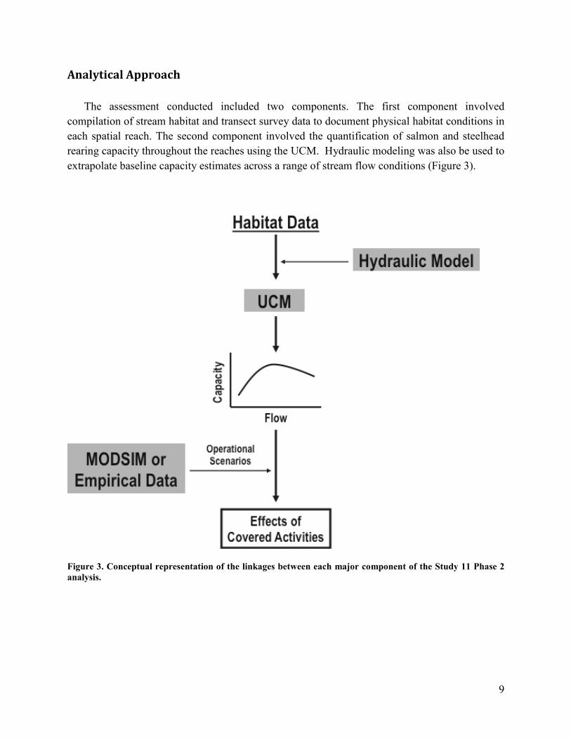
The assessment conducted included two components. The first component involved compilation of stream habitat and transect survey data to document physical habitat conditions in each spatial reach. The second component involved the quantification of salmon and steelhead rearing capacity throughout the reaches using the UCM. Hydraulic modeling was also be used to extrapolate baseline capacity estimates across a range of stream flow conditions (Figure 3).

Figure 3. Conceptual representation of the linkages between each major component of the Study 11 Phase 2 analysis.

10

Unit Characteristic Method Description

The UCM relies on standard stream habitat survey data, typical of most federal and state agency protocols. Carrying capacity (the maximum number of fish that can be supported by available habitat) is a function of the types of habitat features that fish require, and how well those requirements can be satisfied by the habitat conditions available in a given stream. To estimate steelhead trout and Chinook salmon carrying capacity in each spatial segment, the low summer/fall flows and high summer temperatures, which coincide with the presence of rearing juveniles, are assumed to be the bottleneck for fish production (Cramer and Ackerman 2009). As noted above, other factors that can potentially limit fish production potential, such as impediments to migration, are dealt with through separate evaluations.

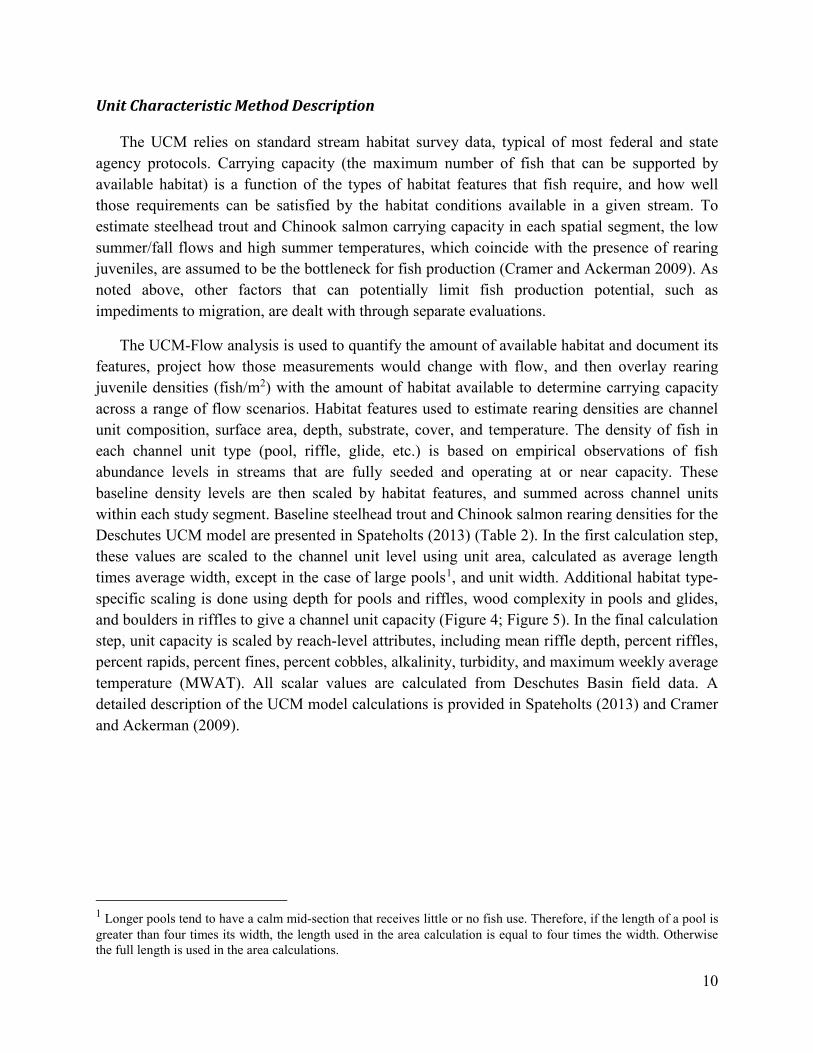
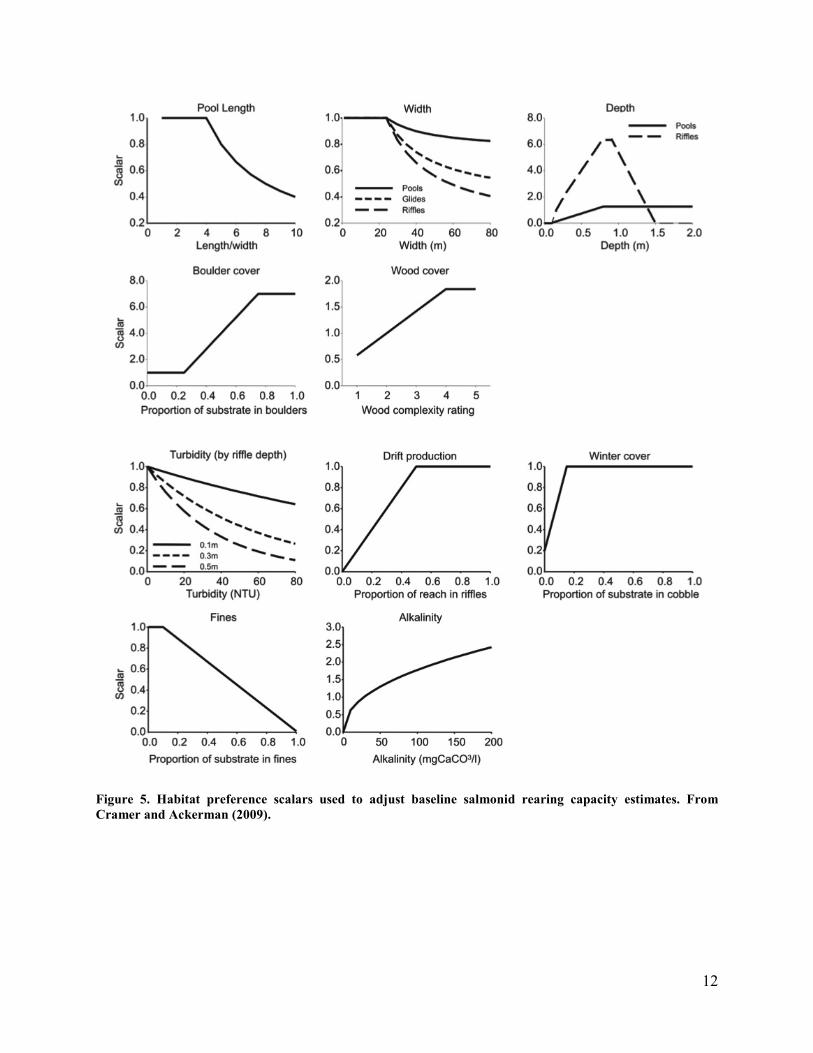
The UCM-Flow analysis is used to quantify the amount of available habitat and document its features, project how those measurements would change with flow, and then overlay rearing juvenile densities (fish/m2) with the amount of habitat available to determine carrying capacity across a range of flow scenarios. Habitat features used to estimate rearing densities are channel unit composition, surface area, depth, substrate, cover, and temperature. The density of fish in each channel unit type (pool, riffle, glide, etc.) is based on empirical observations of fish abundance levels in streams that are fully seeded and operating at or near capacity. These baseline density levels are then scaled by habitat features, and summed across channel units within each study segment. Baseline steelhead trout and Chinook salmon rearing densities for the Deschutes UCM model are presented in Spateholts (2013) (Table 2). In the first calculation step, these values are scaled to the channel unit level using unit area, calculated as average length times average width, except in the case of large pools1, and unit width. Additional habitat type-specific scaling is done using depth for pools and riffles, wood complexity in pools and glides, and boulders in riffles to give a channel unit capacity (Figure 4; Figure 5). In the final calculation step, unit capacity is scaled by reach-level attributes, including mean riffle depth, percent riffles, percent rapids, percent fines, percent cobbles, alkalinity, turbidity, and maximum weekly average temperature (MWAT). All scalar values are calculated from Deschutes Basin field data. A detailed description of the UCM model calculations is provided in Spateholts (2013) and Cramer and Ackerman (2009).

1 Longer pools tend to have a calm mid-section that receives little or no fish use. Therefore, if the length of a pool is greater than four times its width, the length used in the area calculation is equal to four times the width. Otherwise the full length is used in the area calculations.

11

Table 2. Standard densities for juvenile steelhead trout and Chinook salmon (parr/m2) by UCM habitat type. From Cramer and Ackerman (2009).

Habitat Type Steelhead Chinook

Pool 0.17 0.24

Riffle 0.03 0.024

Glide 0.08 0.07

Rapid 0.07 0.024

Cascade 0.03 0.024

Beaver Pond 0.07 0.19

Backwater 0.05 0.13

Figure 4. Diagram of UCM model inputs and rearing capacity scalar calculations.

12

Figure 5. Habitat preference scalars used to adjust baseline salmonid rearing capacity estimates. From Cramer and Ackerman (2009).

13

Temperature Effects on Carrying Capacity

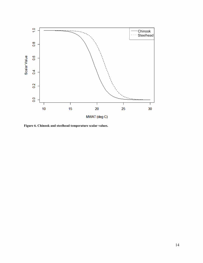
Ackerman et al. (2007) conducted an extensive literature review of the effects of temperature on salmonid rearing densities and independently conducted an analysis of state agency data. The literature review and analysis concluded that densities begin to decrease at a maximum weekly average temperature (MWAT) of 16°C and at a MWAT of 23°C streams lose the ability to rear juvenile salmonids unless thermal refugia are available (Ackerman et al. 2007), consistent with the findings of Sullivan et al. (2000). Low sample size and variability in the data make the form of the decreasing slope in densities between the lower and upper thresholds difficult to ascertain, but the data suggest that for most salmonids, mean densities at an MWAT of 20°C are approximately 30% of those at optimal temperatures. Ackerman et al. (2007) used a logistic function to describe a decrease in maximum expected salmonid rearing capacity at temperatures exceeding 16°C, fitting it through values of 0.95 at MWAT 16°C and 0.05 at MWAT 23°C (Figure 6).

A slightly modified interior Columbia Basin redband-steelhead (O. mykiss gairdneri) temperature scalar has been subsequently developed to more closely mirror temperature tolerances of native redband trout (Courter et al. 2014). Redband trout can withstand higher temperatures and have been observed actively feeding at 26-28°C (Cassinelli and Moffit 2010). The temperature scalar documented in Ackerman et al. (2007) was adjusted conservatively two degrees higher for the redband-steelhead UCM model, so that the beginning of the decrementing density curve began at 18°C. A logistic function was fit through values of 0.95 at MWAT 18°C and 0.05 at MWAT 25°C (Figure 6).

The two temperature scalar options available for use in the UCM model can be described by the following equation:

𝑇𝑇𝑇𝑇𝑖𝑖 =1

1 + 𝑒𝑒−𝑎𝑎−𝑏𝑏𝑇𝑇𝑖𝑖

Where:

Tsi = Temperature scalar for capacity for reach i in a given week.

a = intercept of logit(Tsi) = 19.63 (Chinook), ; 18.1 (steelhead) b = slope of logit(Tsi) = -0.98 (Chinook), ; -0.84 (steelhead)

T = MWAT for reach i in a given week. This scalar was multiplied by the baseline habitat carrying capacity for rearing in each reach of DBHCP analysis.

14

Figure 6. Chinook and steelhead temperature scalar values.

15

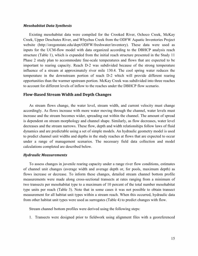
Mesohabitat Data Synthesis

Existing mesohabitat data were compiled for the Crooked River, Ochoco Creek, McKay Creek, Upper Deschutes River, and Whychus Creek from the ODFW Aquatic Inventories Project website (http://oregonstate.edu/dept/ODFW/freshwater/inventory). These data were used as inputs for the UCM-flow model with data organized according to the DBHCP analysis reach structure (Table 1), which is expanded from the initial reach structure presented in the Study 11 Phase 2 study plan to accommodate fine-scale temperatures and flows that are expected to be important to rearing capacity. Reach D-2 was subdivided because of the strong temperature influence of a stream at approximately river mile 130.4. The cool spring water reduces the temperature in the downstream portion of reach D-2 which will provide different rearing opportunities than the warmer upstream portion. McKay Creek was subdivided into three reaches to account for different levels of inflow to the reaches under the DBHCP flow scenario.

Flow-Based Stream Width and Depth Changes

As stream flows change, the water level, stream width, and current velocity must change accordingly. As flows increase with more water moving through the channel, water levels must increase and the stream becomes wider, spreading out within the channel. The amount of spread is dependent on stream morphology and channel shape. Similarly, as flow decreases, water level decreases and the stream narrows. These flow, depth and width relationships follow laws of fluid dynamics and are predictable using a set of simple models. An hydraulic geometry model is used to predict channel unit widths and depths in the study reaches at flows that are expected to occur under a range of management scenarios. The necessary field data collection and model calculations completed are described below.

Hydraulic Measurements

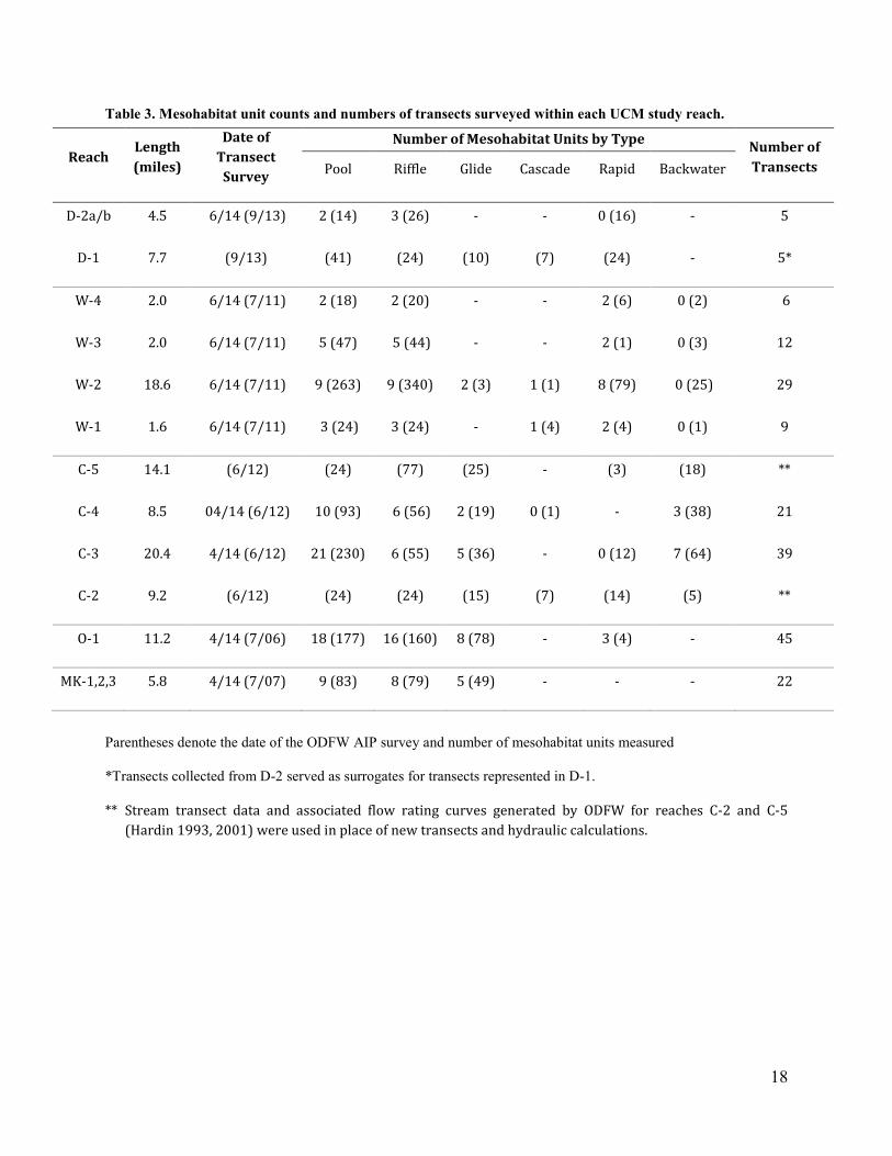
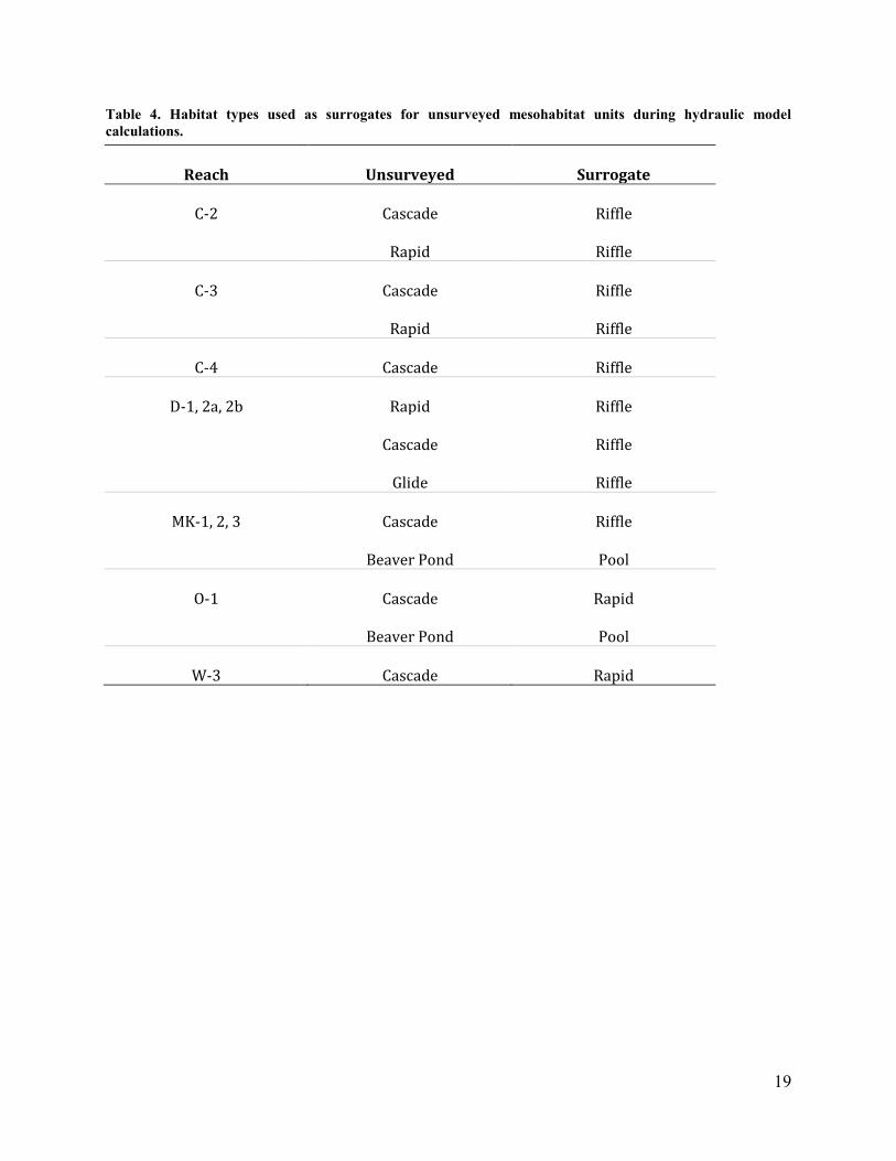
To assess changes in juvenile rearing capacity under a range river flow conditions, estimates of channel unit changes (average width and average depth or, for pools, maximum depth) as flows increase or decrease. To inform these changes, detailed stream channel bottom profile measurements were made along cross-sectional transects at rates ranging from a minimum of two transects per mesohabitat type to a maximum of 10 percent of the total number mesohabitat type units per reach (Table 3). Note that in some cases it was not possible to obtain transect measurement for all habitat unit types within a stream reach. When this occurred, hydraulic data from other habitat unit types were used as surrogates (Table 4) to predict changes with flow.

Stream channel bottom profiles were derived using the following steps:

1. Transects were designed prior to fieldwork using alignment files with a georeferenced

16

aerial image in Trimble Business Center2. Design location adjustments were made in the field with the Trimble Access software in a TSC3 data collector to ensure straight transects across the river without the use of strings or ropes. Upon arrival at each data collection location, transects were established perpendicular to stream flow using a Trimble R8 GPS unit to determine elevations at the right and left bankfull positions. Bankfull positions were visually identified in the field via absence of perennial vegetation and/or the highest mineral-stain line on bedrock and boulder substrate. Both are good indicators of the 1.5-year high water line, an important benchmark for hydraulic model calculations. The 1.5-year return peak flow, as derived from an annual maximum flood series, has been identified as an hydrologic metric that can be used as an estimate of the bankfull flow and effective discharge magnitudes (Dunne and Leopold 1978; Leopold 1994; Leopold et al. 1995);

2. A channel bottom profile was developed by wading from left bank to right bank along each transect and taking elevation measurements with the Trimble at intervals across the full width of the transect with sufficient frequency to capture the bottom variation (more for rocky and less for smooth bottom types). One depth recording was taken at the channel thalweg of each transect. The maximum depth of pools was measured as well as the downstream hydraulic control depth of each pool. Both pool depths were georeferenced to a common elevation point for use in assessing the stage of zero flow, residual pool depth, and potential pool elevations due to backwater effects at different stream flow conditions. Measurements were taken by wading where depth was up to 3.5 feet. Where depths exceeded 3.5 feet at a transect location, an inflatable kayak was used to traverse the transect with the Trimble R8 and Swoffer meter, following the same protocol used for wading except that fixed interval was not employed for either the individual stream profile transects or the stream discharge measurement transects. Rather, depths and velocities were collected and entered into the Trimble at intervals sufficient to capture the shape and bottom variation of the channel. Channel profile and discharge calculations were made based on the horizontal distance between each vertical measurement, regardless of the width. Stream transect data were reviewed in Trimble Business Center and checked for accuracy prior to analysis.

a. For the channel profile measurements, vertical elevations were taken whenever there was any material change in the slope of the bed. Between these points, the number of verticals depended on the substrate characteristics and streambed evenness.

2 Survey utilized Oregon State Plane South Zone 4602 Nad 83/2011 units in International Feet. Vertical Datum in NAVD 88 (geoid 2012a).

17

b. The frequency of vertical elevations was dictated by the following:

i. Very uneven surfaces 1 foot/vertical ii. Cobble - Boulder 2 feet/vertical

iii. Gravel – Cobble 3 feet/vertical iv. Silt – Sand 4 feet/vertical

c. At major boulders, elevation measurements were taken at both sides and on top of

the boulder.

3. Time-stamped water surface elevations (WSEs) were recorded at the right and left wetted edges of the channel at each transect. Vertical measurements continued along the dry portion of the channel from the water’s edge to the bankfull channel width to provide data to model channel widths and depths at flows higher than those during the field survey.

18

Table 3. Mesohabitat unit counts and numbers of transects surveyed within each UCM study reach.

Reach Length (miles)

Date of Transect

Survey

Number of Mesohabitat Units by Type Number of Transects Pool Riffle Glide Cascade Rapid Backwater

D-2a/b 4.5 6/14 (9/13) 2 (14) 3 (26) - - 0 (16) - 5

D-1 7.7 (9/13) (41) (24) (10) (7) (24) - 5*

W-4 2.0 6/14 (7/11) 2 (18) 2 (20) - - 2 (6) 0 (2) 6

W-3 2.0 6/14 (7/11) 5 (47) 5 (44) - - 2 (1) 0 (3) 12

W-2 18.6 6/14 (7/11) 9 (263) 9 (340) 2 (3) 1 (1) 8 (79) 0 (25) 29

W-1 1.6 6/14 (7/11) 3 (24) 3 (24) - 1 (4) 2 (4) 0 (1) 9

C-5 14.1 (6/12) (24) (77) (25) - (3) (18) **

C-4 8.5 04/14 (6/12) 10 (93) 6 (56) 2 (19) 0 (1) - 3 (38) 21

C-3 20.4 4/14 (6/12) 21 (230) 6 (55) 5 (36) - 0 (12) 7 (64) 39

C-2 9.2 (6/12) (24) (24) (15) (7) (14) (5) **

O-1 11.2 4/14 (7/06) 18 (177) 16 (160) 8 (78) - 3 (4) - 45

MK-1,2,3 5.8 4/14 (7/07) 9 (83) 8 (79) 5 (49) - - - 22

Parentheses denote the date of the ODFW AIP survey and number of mesohabitat units measured

*Transects collected from D-2 served as surrogates for transects represented in D-1.

** Stream transect data and associated flow rating curves generated by ODFW for reaches C-2 and C-5 (Hardin 1993, 2001) were used in place of new transects and hydraulic calculations.

19

Table 4. Habitat types used as surrogates for unsurveyed mesohabitat units during hydraulic model calculations.

Reach Unsurveyed Surrogate

C-2 Cascade Riffle

Rapid Riffle

C-3 Cascade Riffle

Rapid Riffle

C-4 Cascade Riffle

D-1, 2a, 2b Rapid Riffle

Cascade Riffle

Glide Riffle

MK-1, 2, 3 Cascade Riffle

Beaver Pond Pool

O-1 Cascade Rapid

Beaver Pond Pool

W-3 Cascade Rapid

20

Stream Flow Measurements Cross-sectional flow transects provide a localized measure of river discharge. For the

DBHCP, at least one flow transect was required for each sampling reach. To account for possible changes in stream flow throughout the day or along a sampling reach, flow transect data were collected at the beginning and end of each field day. Transects were located to ensure downstream flow across the full width of the stream (no eddy or backflow) and to avoid in-river obstacles – that could impair the field crew’s ability to maintain regular measurement intervals. In general, discharge measurement transects were located in areas with uniform depth (e.g., shallow glides or riffle/tail-crests), downstream flow across the entire wetted width, and as few obstacles as possible.

A minimum of one stream flow (Q, discharge) measurement was collected for each study reach where flow was relatively consistent. Flow measurements were extended to upstream and downstream transects as long as there was no change in flow between the transects. New discharge measurements occurred when observed flow conditions changed in the study reach because of tributary input, active diversion, return point, apparent groundwater infusion or other steam inflows. Points of input and diversion were identified during stream reconnaissance prior to data collection.

Velocity measurements were collected at each bottom profile depth vertical across discharge measurement transects. Time-averaged flow measurements were collected using a Marsh-McBirney flow meter and recorded directly into a Trimble R8 and synchronized with depth measurements. The sampling methodology was as follows:

1. After selecting a suitable site, a transect was established in the same manner as all other transects perpendicular to stream flow using a Trimble R8 GPS unit to determine elevations at the right and left bankfull positions.

2. Sample intervals were obtained via the same method used for channel profile transects.

3. Velocity measurements were taken at 20% and 80% of stream depth when depth exceeded 0.6 meters, and at 60% of stream depth when depth ≤ 0.6 meters.

To establish a rating curve (flow level versus stream discharge) for each transect, the model was calibrated to the hydraulic conditions of measured WSE and flow using HEC-RAS, a widely-used hydraulic model developed by the U. S. Army Corps of Engineers (HEC 2010). The channel roughness, represented by the equivalent roughness, was calculated for the measured WSE and flow. The equivalent roughness, a constant value for the transect, was then used in the HEC-RAS model to estimate WSEs for each of the 30 flows on the rating curve. With WSE available, hydraulic radius and other parameters could be derived accordingly. This process was used as a quality control procedure to ensure the channel roughness (i.e., Manning’s n values)

21

decreased with increasing flows. A range, encompassing 30 flows for each study reach, was developed to address the flows of interest for assessing fish habitat conditions with the UCM-Flow Model.

During hydraulic model calibration, a study reach was divided into two or more sub-reaches if the channel gradient varied significantly such that a single-reach model could not adequately capture the hydraulic variations in the vicinity of where the gradient changes. An average slope based on the measured WSEs of the transects available within the sub-reach was used as the downstream boundary condition in the model.

Ideally, the calibration process would rely on two or three pairs of WSE vs. flow measurements. However, hydraulic modeling is possible using the estimation principles described above with only one (WSE vs. Q) measurement generated during stream bottom profiling surveys. This was the approach taken for our analysis.

Hydraulic Calculations

Hydraulic modeling using HEC-RAS integrates the channel transect measurements and generates the following information with incremental changes in stream channel parameters relative to streamflow for each habitat type. These parameters include:

- Width (wetted) - Depth (average and maximum) - Velocity (average and maximum) - Elevation (Stage – relative to localized benchmark) - Toe Width - Wetted Perimeter - Slope - Manning’s N - Froude # - Area (wetted; cross-sectional conveyance area not surface area)

The HEC-RAS model output was then used to estimate the increase in surface area of habitat units and approximate the average width and depth of each habitat unit for a broad range of flow conditions3. Because the UCM model uses channel unit area and depth to determine rearing capacity values, surface area and depth are the parameters of interest for the UCM-Flow analyses.

3 Maximum depth is used to scale carrying capacity in pools. Average depth is used to scale capacity in all other mesohabitat types.

22

Estimate of Bankfull Flow / Transect Relative Benchmark

Bankfull flow is assumed to be a peak flow with a 1.5-year recurrence interval (Leopold 1994). Flow gauging data nearest to the study reach in question were used to calculate a 1.5-year recurrence interval to establish a bankfull flow level for each cross-channel transect, which was later used as a reference point for the hydraulic modeling described above. Calculated bankfull flow estimates were validated to ensure consistency. As an example, the Froude number calculated at bankfull flow had to be less than one (subcritical flow), and greater than the Froude numbers under lower flow conditions.

Field Data Collection and Analysis

Data collection began with the Crooked River, Ochoco Creek and McKay Creek in accordance with the numbers of transects specified in Table 3. Hydraulic analyses was then conducted for half the transects selected to represent all reaches and mesohabitats types.

Prior to the collection of transect data in the Deschutes River and Whychus Creek, the AIP data were evaluated for variation in water depth and width within mesohabitats types. The results of this evaluation indicated that a transect sample size of 5% of the habitat units would be adequate to capture the variance in stream morphology, the number of transects was therefore reduced accordingly from the minimum numbers shown in Table 3.

Water Management Scenario Descriptions

Fish production potential was calculated for a number of different flow and temperature regimes in the waters covered by the DBHCP (Table 5). Current conditions in the Deschutes River, Whychus Creek, Crooked River, and Ochoco Creek were represented by the “Existing Flow” scenario developed by Oregon Department of Environmental Quality (ODEQ) for Heat Source modeling of peak surface water temperatures (ODEQ 2014). The Existing Flow scenario reflects late summer (July-August) instream flows with all existing land use conditions and all ongoing uses of water in the basin, including the storage, release, diversion and return of irrigation water and withdrawal of water for municipal and domestic uses. These are average flows reported at existing gages during the specific years for which Heat Source was run (2000 for Whychus Creek, 2001 for the Deschutes River, and 2005 for the Crooked River and Ochoco Creek).

Two reference conditions were evaluated; “Natural Flow” and Unregulated Flow”. The Natural Flow scenario was also developed by ODEQ as a reference condition in the Heat Source modeling. It represents instream flows with current land use but no consumptive use of water, at the 50 percent exceedance level for the August monthly average natural flow, as estimated in Oregon Water Resources Department Water Availability Analysis. The Unregulated Flow scenario is comparable to the Natural Flow scenario, but was developed specifically for the DBHCP analysis. The Unregulated flows are the 80 percent exceedance levels for monthly

23

average flows in August (historically the driest month in the basin) with no storage, release, diversion or return of irrigation water and no municipal withdrawal. In most cases, Natural flows and Unregulated flows are similar. Both scenarios were evaluated for all waters except the Deschutes River. The differences between the two scenarios for the Deschutes River were relatively minor, so only the Unregulated Flow scenario was evaluated.

Multiple scenarios related to future flows under the DBHCP were also evaluated. For all waters, the “DBHCP Minimum Flow” was addressed. This represents the minimum instream flow that would be provided under the DBHCP conservation measures proposed as of August 2014. In many cases, instream flows would be higher than the minimums specified in the proposed conservation measures, but the minimum guaranteed flows were used in the UCM-Flow calculations to be conservative. Additional DBHCP flow scenarios were evaluated for some waters, such as the Deschutes River where the minimum instream flow will increase in increments over time. These scenarios are given descriptive names to clarify the flows they represent. Readers should reference Chapter 5 of the DBHCP for additional detail about development of the flow management scenarios.

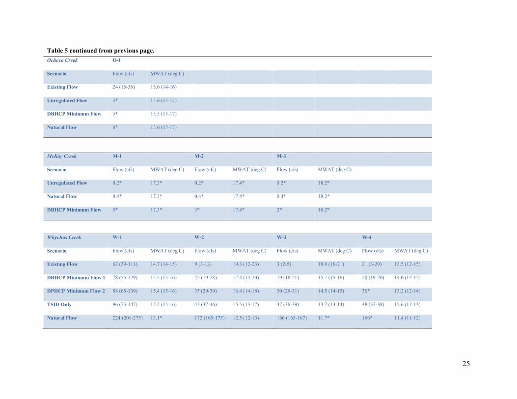
Average flow and temperature (MWAT) conditions were calculated for each stream reach and flow management scenario. The full range of flows and temperatures predicted by Heat Source longitudinally within each reach are also provided in parentheses in Table 5. This range reflects the effects of downstream temperature inputs due to meteorological conditions and spring water accretion. Although averaging temperature and flow conditions reduces the spatial resolution at which these variables are being quantified in the UCM-Flow model, additional spatial complexity would be unlikely to yield a marked relative change in predicted fish capacity between management scenarios. Therefore, the existing reach structure was assumed to be an adequate spatial construct for calculating flow and temperature metrics.

24

Table 5: Average flows and MWAT values used for each DBHCP scenario within each reach in the UCM analyses. Range in values in parentheses. Crooked River C-2 C-3 C-4 C-5

Scenario Flow (cfs) MWAT (deg C) Flow (cfs) MWAT (deg C) Flow (cfs) MWAT (deg C) Flow (cfs) MWAT (deg C)

Existing Flow 54 (36-74) 19.4 (19-20) 109 (36-120) 20.3 (19-21) 66 (59-71) 17.4 (15-19) 205 (58-226) 12.3 (10-15)

Natural Flow 79* 20.9* 69 (52-79) 22.5 (21-25) 52* 24.0 (23-25) 52* 21.6 (21-23)

Unregulated Flow 35* 20.3 (19-21) 28 (23-35) 22.2 (20-26) 23* 25.2 (24-26) 23* 21.2 (21-24)

DBHCP Minimum Flow 51 (33-71) 19.2 (19-20) 36 (27-48) 21.4 (20-22) 36 (26-39) 20.2 (18-22) 93 (24-104) 14.4 (10-19)

Deschutes River D-1 D-2a D-2b

Scenario Flow (cfs) MWAT (deg C) Flow (cfs) MWAT (deg C) Flow (cfs) MWAT (deg C)

Existing Flow 412 (254-532) 14.0 (13-15) 249 (192-254) 14.7 (15-16) 109 (91-119) 19.5 (19-21)

DBHCP Minimum Flow 1 (109 cfs at RM 159)

467 (310-579) 14.5 (14-16) 304 (247-310) 15.4 (15-16) 164 (146-174) 19.1 (19-20)

DBHCP Minimum Flow 2 (139 cfs at RM 159)

497 (339-608) 14.6 (14-16) 334 (278-339) 15.5 (15-16) 194 (176-204) 18.9 (19-20)

DBHCP Minimum Flow 3 (159 cfs at RM 159)

517 (359-628) 14.7 (14-16) 354 (298-360) 15.7 (15-16) 214 (197-224) 18.8 (18-19)

DBHCP Minimum Flow 4 (169 cfs at RM 159)

527 (369-638) 14.8 (14-16) 364 (308-370) 15.7 (16-17) 224 (207-234) 18.7 (18-19)

DBHCP Minimum Flow 5 (209 cfs at RM 159)

567 (410-678) 15.0 (14-16) 404 (348-410) 15.9 (16-17) 264 (247-274) 18.5 (18-19)

DBHCP Minimum Flow 6 (233 cfs at RM 159)

591 (434-702) 15.0 (14-16) 428 (372-434) 16.0 (16-17) 288 (271-299) 18.3 (18-19)

18 C Target (330 cfs) 688 (531-799) 15.3 (15-16) 525 (469-531) 16.2 (16-17) 385 (368-395) 18.0*

ODEQ Natural 1730 (1502-1903) 15.8 (15-17) 1496 (1439-1502) 16.4 (16-17) 1355 (1338-1366) 16.9*

*No range in value

25

Table 5 continued from previous page. Ochoco Creek O-1

Scenario Flow (cfs) MWAT (deg C)

Existing Flow 24 (16-36) 15.0 (14-16)

Unregulated Flow 3* 15.6 (15-17)

DBHCP Minimum Flow 5* 15.5 (15-17)

Natural Flow 6* 15.6 (15-17)

McKay Creek M-1 M-2 M-3

Scenario Flow (cfs) MWAT (deg C) Flow (cfs) MWAT (deg C) Flow (cfs) MWAT (deg C)

Unregulated Flow 0.2* 17.3* 0.2* 17.4* 0.2* 18.2*

Natural Flow 0.4* 17.3* 0.4* 17.4* 0.4* 18.2*

DBHCP Minimum Flow 5* 17.3* 3* 17.4* 2* 18.2*

Whychus Creek W-1 W-2 W-3 W-4

Scenario Flow (cfs) MWAT (deg C) Flow (cfs) MWAT (deg C) Flow (cfs) MWAT (deg C) Flow (cfs) MWAT (deg C)

Existing Flow 62 (39-113) 14.7 (14-15) 9 (3-12) 19.3 (12-23) 3 (2-5) 18.0 (16-21) 21 (3-29) 13.5 (12-15)

DBHCP Minimum Flow 1 78 (55-129) 15.5 (15-16) 25 (19-28) 17.4 (14-20) 19 (18-21) 15.7 (15-16) 20 (19-20) 14.0 (12-15)

DPHCP Minimum Flow 2 88 (65-139) 15.4 (15-16) 35 (29-39) 16.4 (14-18) 30 (29-31) 14.5 (14-15) 30* 13.2 (12-14)

TSID Only 96 (73-147) 15.2 (15-16) 43 (37-46) 15.5 (13-17) 37 (36-39) 13.7 (13-14) 38 (37-38) 12.6 (12-13)

Natural Flow 224 (201-275) 13.1* 172 (165-175) 12.5 (12-13) 166 (165-167) 11.7* 166* 11.4 (11-12)

26

Spawning Habitat Analysis Potential spawning production is estimated using the proportion of the channel unit area

comprised of gravels and fines in the stream bed along with species-specific minimum depth, redd and defended territory area, species-specific number of eggs per redd, and estimates of survival from egg to parr. Spawnable gravels were not explicitly measured during AIP surveys, but estimates of spawnable area were needed. To accomplish this, mesohabitat area was scaled by percent gravel substrate. For example, if a channel unit has 25% gravel substrate the spawnable area could be as much as 25% of the area available. However, not all gravels are the appropriate size for spawning, so the area was reduced by an arbitrary value of 50% to roughly account for this factor. In the previous case, the spawnable area would be 12.5% of the channel unit area. Spawning was assessed using DBHCP Minimum flows in Crooked River (Table 6) and Ochoco Creek (4.1 cfs 4) during the non-irrigation season because these conditions represent the lowest flow conditions that would be encountered by an adult salmon or steelhead. Conversely, summer flow conditions in McKay Creek, Whychus Creek and the Deschutes River would be limiting because summer flows are lowest in these unregulated streams. Results from hydraulic modeling were used to estimate channel unit area, depth, and subsequent potential spawning areas for steelhead trout and Chinook salmon.

For this portion of our analysis, parr production potential was based on the area available for redd deposition, adult spawner defended territory size, eggs deposited per redd, and egg-to-parr survivorship. Modeling assumptions included redd and defended territory sizes of 4 yd2 and a minimum depth of 6 inches for steelhead and 24 yd2 with a minimum depth of 12 inches for Chinook. The number of redds was estimated as the number of whole redds and defended territory area available. Each steelhead redd was assumed to contain 2,800 eggs and each Chinook redd 5,000 eggs. Egg-to-parr survivorship was 5.85% for both steelhead and Chinook giving a potential parr produced per redd of 163 for steelhead and 292 for Chinook.

Fine sediment substrates reduce water flow through redds, which reduces egg survival. In the spawning analysis, juvenile production is reduced when fines represent more than 25% of the available substrate sediments. This reduction continues linearly down to zero at 55% fines. Percent fines for each channel unit in the AIP data were used as an estimate of fines in gravels. This scalar was applied to the redd-based production to calculate total potential spawning production values.

4 Represents the average flow condition under the DBHCP flow scenario in Ochoco Creek (rkm 0-18.2) as modeled by Heat Source from November through March.

27

Table 6: DBHCP minimum non-irrigation flows in the Crooked River used in spawning analyses.

C-2 C-3 C-4 C-5

Normal Year 100.5 89.9 75 75

Dry Year 55.5 44.8 30 30

Fish Passage Assessment

This section header is a placeholder. Further work is being carried out to quantify passage conditions.

28

Results

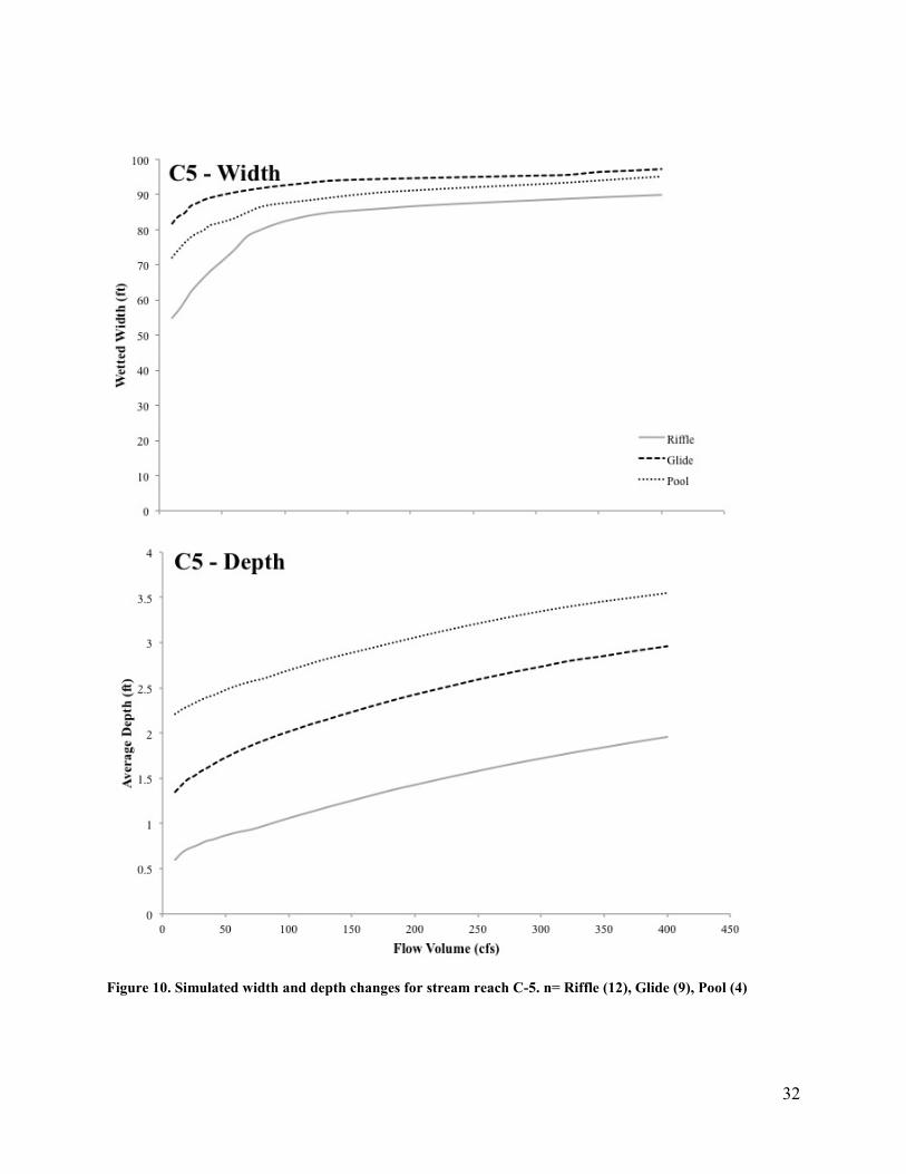
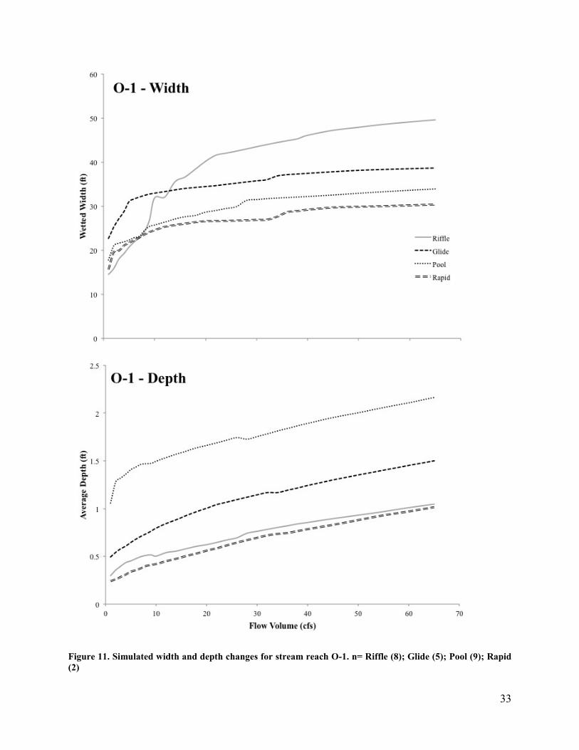
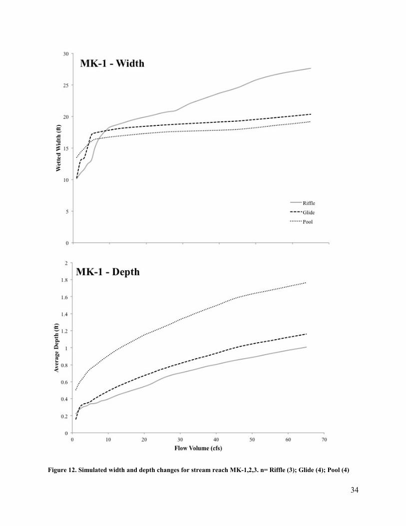
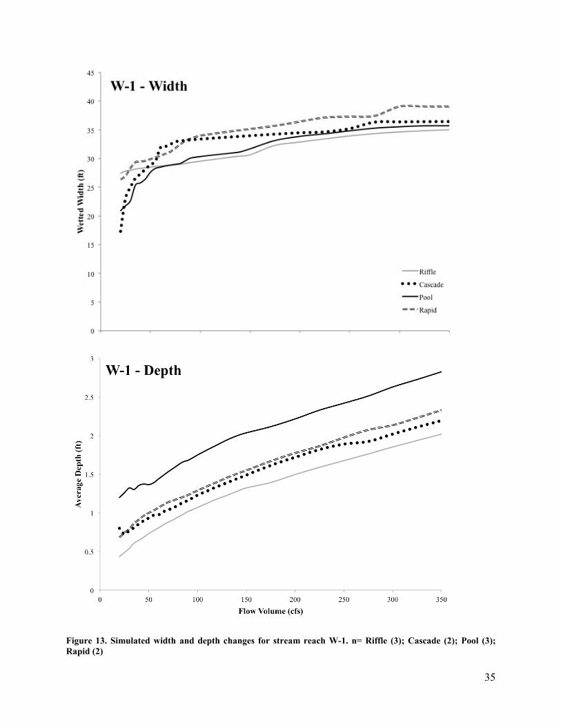
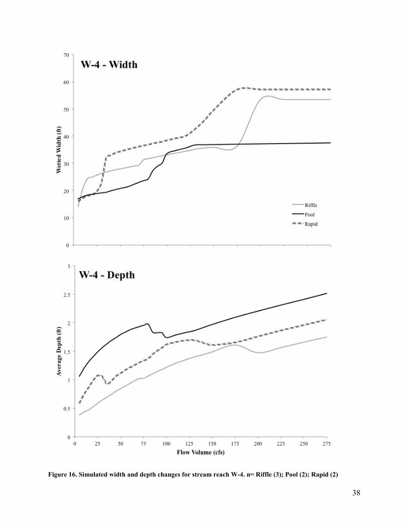
Flow-Based Stream Width and Depth Changes Figures 7-17 provide width and depth predictions simulated using the HEC-RAS model. In

most cases, average width and depth increased as expected across the full range of increasing stream flow. However, predicted average width or depth of a cross section decreased when stream flow increased for some habitat types (Figures 13-14). In these cases there is a bench in the cross sectional profile. When flow levels exceed the bench elevation, the stream width rapidly expands with many points of relatively shallow water. Under these situations, the average depth across the transect decreased. Thalweg depths always increase with increasing flows, but sometimes the average depth may be reduced compared to averages at lower flows.

29

Figure 7. Simulated width and depth changes for stream reach C-2. n= Riffle (6), Glide (6), Pool (6)

30

Figure 8. Simulated width and depth changes for stream reach C-3. n= Riffle (3), Glide (5), Pool (10), Backwater (4)

31

Figure 9. Simulated width and depth changes for stream reach C-4. n= Riffle (4), Glide (2), Pool (5), Backwater (2)

32

Figure 10. Simulated width and depth changes for stream reach C-5. n= Riffle (12), Glide (9), Pool (4)

33

Figure 11. Simulated width and depth changes for stream reach O-1. n= Riffle (8); Glide (5); Pool (9); Rapid (2)

34

Figure 12. Simulated width and depth changes for stream reach MK-1,2,3. n= Riffle (3); Glide (4); Pool (4)

35

Figure 13. Simulated width and depth changes for stream reach W-1. n= Riffle (3); Cascade (2); Pool (3); Rapid (2)

36

Figure 14. Simulated width and depth changes for stream reach W-2. n= Riffle (9); Glide (2); Cascade (2); Pool (9); Rapid (8)

37

Figure 15. Simulated width and depth changes for stream reach W-3. n= Riffle (5); Pool (5); Rapid (2)

38

Figure 16. Simulated width and depth changes for stream reach W-4. n= Riffle (3); Pool (2); Rapid (2)

39

Figure 17. Simulated width and depth changes for stream reach D-1 and D-2. n= Riffle (3); Pool (2)

40

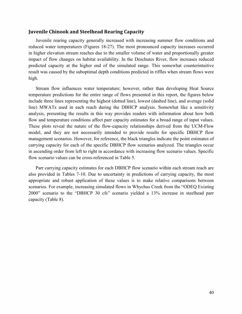
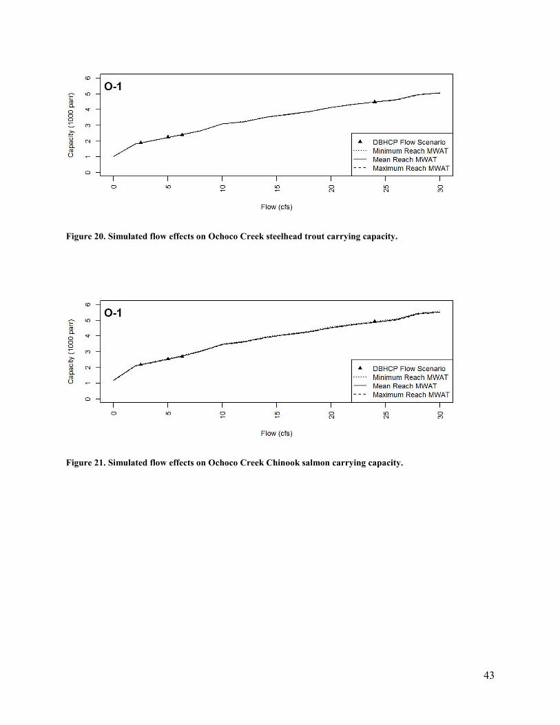
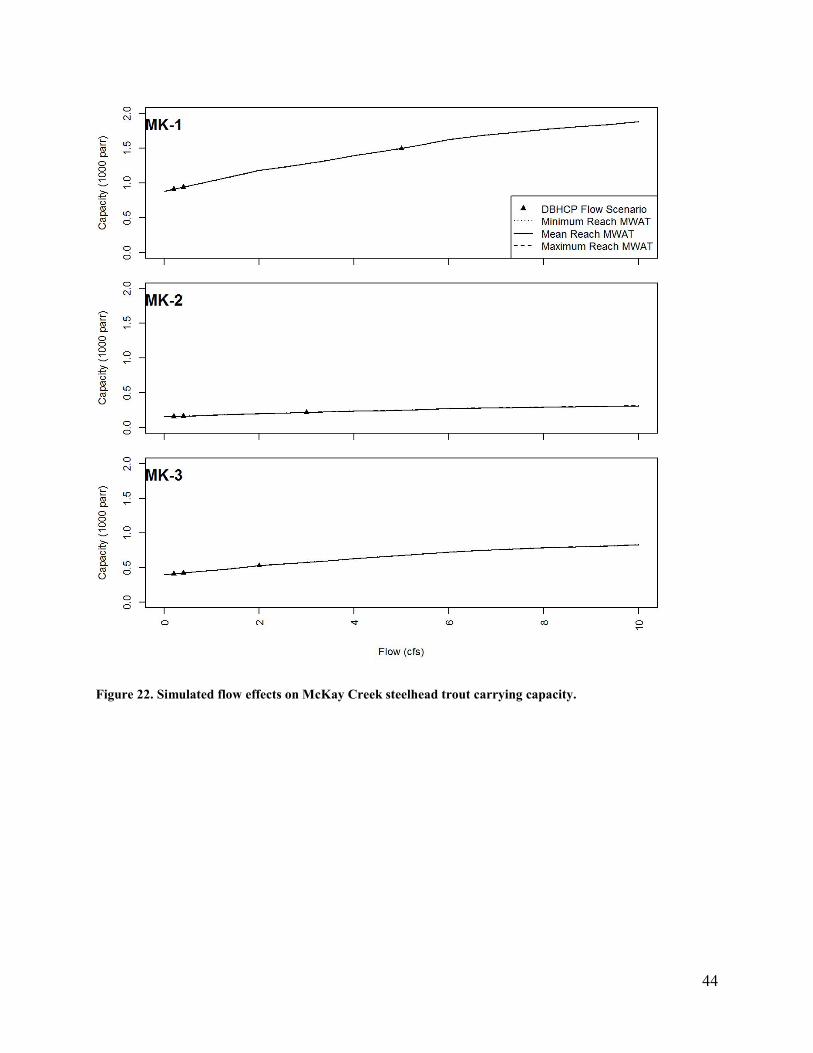
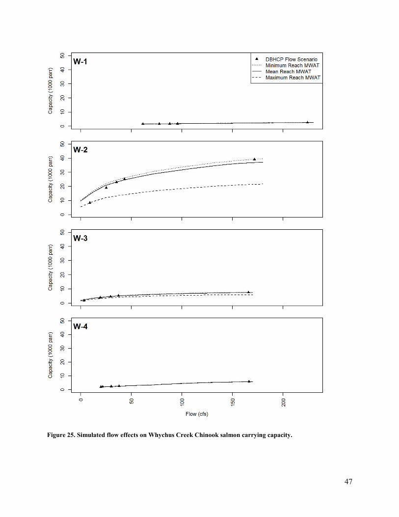
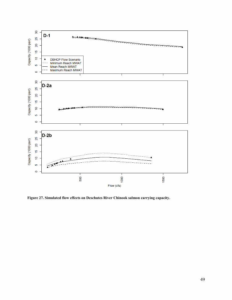
Juvenile Chinook and Steelhead Rearing Capacity Juvenile rearing capacity generally increased with increasing summer flow conditions and

reduced water temperatures (Figures 18-27). The most pronounced capacity increases occurred in higher elevation stream reaches due to the smaller volume of water and proportionally greater impact of flow changes on habitat availability. In the Deschutes River, flow increases reduced predicted capacity at the higher end of the simulated range. This somewhat counterintuitive result was caused by the suboptimal depth conditions predicted in riffles when stream flows were high.

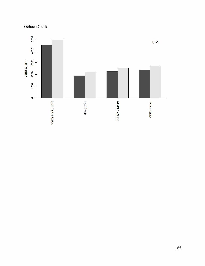
Stream flow influences water temperature; however, rather than developing Heat Source temperature predictions for the entire range of flows presented in this report, the figures below include three lines representing the highest (dotted line), lowest (dashed line), and average (solid line) MWATs used in each reach during the DBHCP analysis. Somewhat like a sensitivity analysis, presenting the results in this way provides readers with information about how both flow and temperature conditions affect parr capacity estimates for a broad range of input values. These plots reveal the nature of the flow-capacity relationships derived from the UCM-Flow model, and they are not necessarily intended to provide results for specific DBHCP flow management scenarios. However, for reference, the black triangles indicate the point estimates of carrying capacity for each of the specific DBHCP flow scenarios analyzed. The triangles occur in ascending order from left to right in accordance with increasing flow scenario values. Specific flow scenario values can be cross-referenced in Table 5.

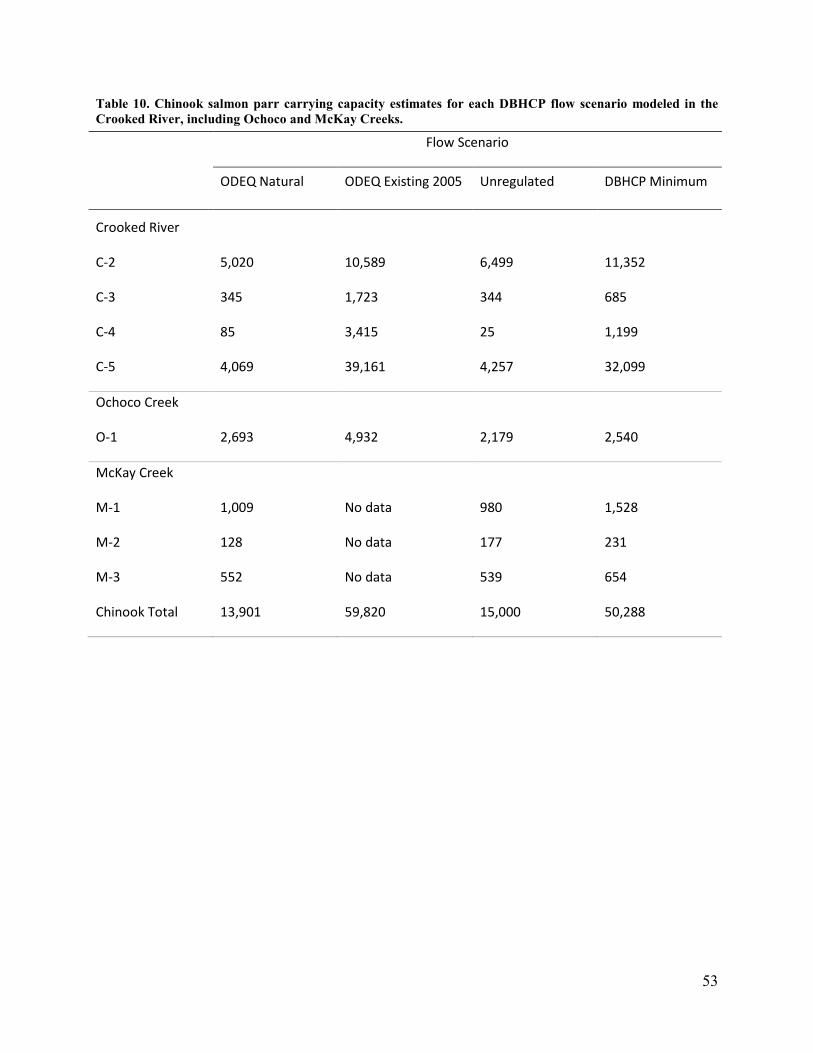
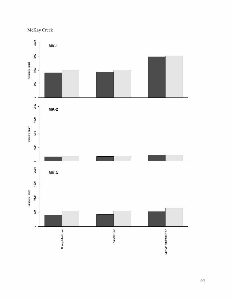
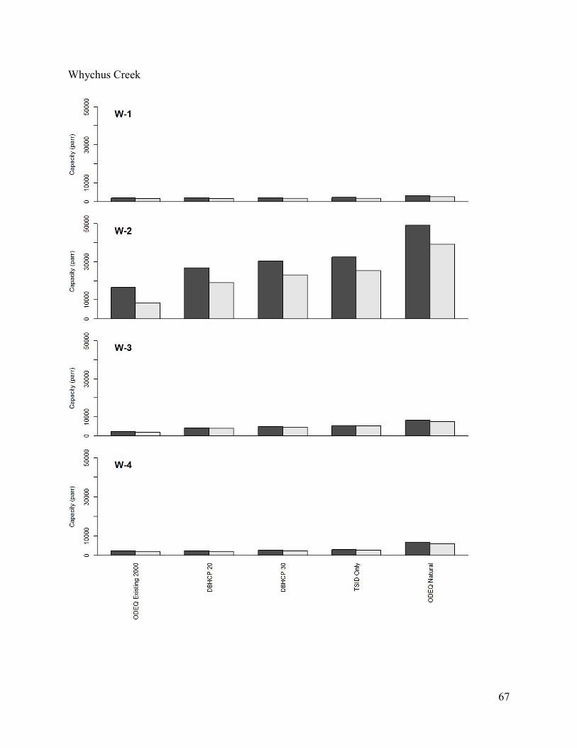
Parr carrying capacity estimates for each DBHCP flow scenario within each stream reach are also provided in Tables 7-10. Due to uncertainty in predictions of carrying capacity, the most appropriate and robust application of these values is to make relative comparisons between scenarios. For example, increasing simulated flows in Whychus Creek from the “ODEQ Existing 2000” scenario to the “DBHCP 30 cfs” scenario yielded a 13% increase in steelhead parr capacity (Table 8).

41

Figure 18. Simulated flow effects on Crooked River steelhead trout carrying capacity.

42

Figure 19. Simulated flow effects on Crooked River Chinook salmon carrying capacity.

43

Figure 20. Simulated flow effects on Ochoco Creek steelhead trout carrying capacity.

Figure 21. Simulated flow effects on Ochoco Creek Chinook salmon carrying capacity.

44

Figure 22. Simulated flow effects on McKay Creek steelhead trout carrying capacity.

45

Figure 23. Simulated flow effects on McKay Creek Chinook salmon carrying capacity.

46

Figure 24. Simulated flow effects on Whychus Creek steelhead trout carrying capacity.

47

Figure 25. Simulated flow effects on Whychus Creek Chinook salmon carrying capacity.

48

Figure 26. Simulated flow effects on Deschutes River steelhead trout carrying capacity.

49

Figure 27. Simulated flow effects on Deschutes River Chinook salmon carrying capacity.

50

Table 7. Chinook salmon and steelhead trout parr carrying capacity estimates for each DBHCP flow scenario modeled in the Deschutes River.

Flow Scenario

ODEQ Natural ODEQ Existing

2001 DBHCP 109 cfs

DBHCP 139 cfs

DBHCP 169 cfs

Steelhead Trout Parr Production

D-1 18,975 28,429 28,254 28,076 27,912

D-2a 11,821 11,590 12,115 12,376 12,622

D-2b 14,295 6,686 8,758 10,041 11,079

Steelhead Total 45,091 46,705 49,127 50,493 51,613

Spring Chinook Parr Production

D-1 18,686 26,529 26,358 26,215 26,044

D-2a 9,425 9,471 9,821 10,015 10,167

D-2b 10,628 3,198 4,668 5,608 6,465

Chinook Total 38,739 39,198 40,847 41,838 42,676

51

Table 8. Chinook salmon and steelhead trout parr carrying capacity estimates for each DBHCP flow scenario modeled in Whychus Creek.

Flow Scenario

ODEQ Natural ODEQ Existing 2000 DBHCP 20 cfs DBHCP 30 cfs

Steelhead Trout Parr Production

W-1 3,266 1,957 2,098 2,205

W-2 49,262 16,490 26,851 30,385

W-3 8,067 2,193 4,096 4,816

W-4 6,884 2,422 2,366 2,777

Steelhead Total 67,479 23,062 35,411 40,183

Spring Chinook Parr Production

W-1 2,658 1,585 1,670 1,758

W-2 39,164 8,389 18,990 22,972

W-3 7,462 1,839 3,909 4,623

W-4 5,837 2,136 2,084 2,422

Chinook Total 55,121 13,949 26,653 31,775

52

Table 9. Steelhead trout parr carrying capacity estimates for each DBHCP flow scenario modeled in the Crooked River, including Ochoco and McKay Creeks.

Flow Scenario

ODEQ Natural ODEQ Existing 2005 Unregulated DBHCP Minimum

Crooked River

C-2 14,937 19,544 15,831 19,837

C-3 1,057 2,837 981 1,524

C-4 330 3,106 101 1,962

C-5 13,390 41,293 12,075 33,411

Ochoco Creek

O-1 2,385 4,484 1,893 2,243

McKay Creek

M-1 940 No data 909 1,492

M-2 167 No data 162 220

M-3 423 No data 410 527

Steelhead Total 33,629 71,264 32,362 61,216

53

Table 10. Chinook salmon parr carrying capacity estimates for each DBHCP flow scenario modeled in the Crooked River, including Ochoco and McKay Creeks.

Flow Scenario

ODEQ Natural ODEQ Existing 2005 Unregulated DBHCP Minimum

Crooked River

C-2 5,020 10,589 6,499 11,352

C-3 345 1,723 344 685

C-4 85 3,415 25 1,199

C-5 4,069 39,161 4,257 32,099

Ochoco Creek

O-1 2,693 4,932 2,179 2,540

McKay Creek

M-1 1,009 No data 980 1,528

M-2 128 No data 177 231

M-3 552 No data 539 654

Chinook Total 13,901 59,820 15,000 50,288

54

Spawning Habitat Analysis The underlying assumption of our analysis is that juvenile rearing is the limiting life-stage for

Chinook and steelhead production in the upper Deschutes Basin. To test this assumption we quantified available spawning habitat within each DBHCP stream reach. Table 7 provides estimates of spawning capacity for both steelhead trout and Chinook salmon in terms of parr equivalents for direct comparison to rearing capacity estimates. For all stream reaches, and for all flow assumptions, spawning capacity far exceeded predicted rearing capacity, affirming our assertion that Chinook and steelhead carrying capacity was juvenile rearing limited.

Table 11. Estimates of spawning capacity converted to parr equivalents.

Stream Reach Redband-Steelhead

(Winter/Spring Flows) Spring Chinook

(Summer/Fall Flows) C-2 Normal 570,681 201,619 C-3 Normal 3,834,600 1,440,394 C-4 Normal 872,581 314,646 C-5 Normal 3,350,785 1,458,533 C-2 Dry 526,350 NA C-3 Dry 3,270,639 NA C-4 Dry 698,818 NA C-5 Dry 2,601,283 NA D-1 NA 458,665 D-2a NA 64,325 D-2b NA 33,951 M-1 NA 20,976 M-2 NA 3,385 M-3 NA 23,440 O-1 220,872 178,962 W-1 NA 60,778 W-2 NA 438,306 W-3 NA 40,071 W-4 NA 49,940

55

Fish Passage Assessment

This section header is a placeholder. Further work is being carried out to quantify passage conditions.

56

References

Ackerman, NK, C Justice, and S Cramer. 2007. Juvenile steelhead carrying capacity of the upper Deschutes Basin 2007 Update. Report prepared by Cramer Fish Sciences for Portland General Electric Company, Portland OR.

Bjornn, T. C., and D. W. Reiser. 1991. Habitat re- quirements of salmonids in streams. Pages 83–138 in W. R. Meehan, editor. Influences of forest and rangeland management on salmo- nid fishes and their habitats. American Fisher- ies Society, Special Publication 19, Bethesda, Maryland.

Burke, JL, KK Jones and JM Dambacher. 2010. Habrate: A limiting factors model for assessing stream habitat quality for salmon and steelhead in the Deschutes River Basin. Information Report 2010-03, Oregon Department of Fish and Wildlife, Corvallis OR. 31pp + app.

Bustard, D. R., and D. W. Narver. 1975. Aspects of winter ecology of juvenile coho salmon (Onco- rhynchus kisutch) and steelhead trout (Salmo gairdneri). Journal of the Fisheries Research Board of Canada 32:667–680.

Cassinelli, John D., Christine M. Moffit. 2010. Comparison of Growth and Stress is Resident Redband Trout Held in Laboratory Simulations of Montane and Desert Summer Temperature Cycles. American Fisheries Society. 139: 339-352.

Conder, AL and TC Annear. 1987. Test of Weighted Usable Area Estimates Derived from a PHABSIM Model for Instream Flow Studies on Trout Streams. North American Journal of Fisheries Management. 7:339-350.

Cramer SP and RCP Beamesderfer. 2006. Population dynamics, habitat capacity, and a life history simulation model for steelhead in the Deschutes River, OR

Cramer SP and K Ceder. 2013. Stream Flows and Potential Production of Spring-Run Chinook Salmon and Steelhead in the Upper South Fork of Battle Creek, California. Cramer Fish Sciences Technical Report.

Cramer SP and NK Ackerman. 2009a. Linking stream carrying capacity for salmonids to habitat features. In: Knudsen E and J Michael (eds) Pacific salmon environmental and life history models. American Fisheries Society Symposium 71, Bethesda MD. pp 225-254

Cramer SP and NK Ackerman. 2009b. Prediction of stream carrying capacity for steelhead (Oncorhyncus mykiss): the Unit Characteristic Method. pp 255-288 In: Knudsen E and J Michael (eds) Pacific salmon environmental life history models. American Fisheries Society Symposium 71, Bethesda MD.

57

Dunne, T., and L.B. Leopold. 1978. Water in environmental planning. W.H. Freeman and Company, San Francisco, California.

Hardin, T. 1993. Crooked River Instream Flow Study. Prepared for ODFW, BLM, and BOR. Oregon Department of Fish and Wildlife, Bend Office by Hardin-Davis, Inc. Albany OR. 18pp + app.

Hardin, T. 2001. Physical habitat for anadromous species in the Crooked River below Bowman Dam. Report prepared for BOR, Boise, ID by Hardin-Davis Inc. Corvallis OR. 4 pp + app.

Hartman, G. F. 1965. The role of behavior in the ecology and interaction of underyearling coho salmon, Oncorhynchus kisutch, and steelhead trout, Salmon gairdneri. Journal of the Fisheries Research Board of Canada 22:1035–1081.

Hillman, T. W., J. S. Griffith, and W. S. Platts. 1987. Summer and winter habitat selection by juvenile Chinook salmon in a highly sedimented Idaho stream. Transactions of the American Fisheries Society 116:185–195.

Hydrologic Engineering Center (HEC). 2010. HEC-RAS River Analysis System User’s Manual, CDP-68. U.S. Army Corps of Engineers Institute of Water Resources Hydrologic Engineering Center. Davis, CA.

LaMarche, J. 2007. Results from 2007 Crooked River Seepage Run. OWRD technical memorandum from Jonathan LaMarche, hydrologist, to K. Gorman, South Central Region Manager dated 2 January 2007.

Leopold, L.B. 1994. A view of the river, Harvard University Press, Cambridge, Massachusetts.

Leopold, L.B., M.G. Wolman, and J.P. Miller. 1995. Fluvial processes in geomorphology. Republication. Dover Publications, Inc. New York, N.Y. 522 p.

National Resources Conservation Service (NRCS). 2010. Preliminary hydraulic analysis and restoration recommendations for the Lower Crooked River, Prineville to Lone Pine. Report submitted to the Crooked River Watershed Council by USDS NRCS, Portland OR February 10, 64 pp.

Nickelson, Thomas; Peter Lawson. 1998. Population viability of coho salmon, Oncorhynchus kisutch, in Oregon coastal basins: application of a habitat-based life cycle model. Canadian Journal of Fisheries and Aquatic Sciences, Vol. 55, Page(s): 2383-2392

Nickelson, Thomas E.; Mario F. Solazzi, Steven L. Johnson, and Jeffrey D. Rodgers. 2012. An approach to determining stream carrying capacity and limiting habitat for Coho Salmon (Oncorhynchus kisutch). Series: Oregon Dept. Fish and Wildlife, Coho Workshop. May 26-28, 1992. Naniamo, B.C., Canada, Page(s): 251-260

58

Nielsen-Pincus, M. 2008. Lower Crooked River Watershed Assessment. Crooked River Watershed Council. Prineville, OR. February 2008. 227pp.

Oregon Department of Fish and Wildlife (ODFW). 1996. Aquatic Inventory Protocol surveys for the Deschutes River reach between Big Falls and Lake Billy Chinook.

Oregon Department of Fish and Wildlife (ODFW). 2006. Aquatic Inventory Protocol surveys for the Crooked River reach between Lone Pine Bridge and People’s Diversion.

Oregon Department of Fish and Wildlife (ODFW). 2012. Aquatic Inventory Protocol surveys for the Crooked River, 2012 surveys, accessed 14 January 2014. http://oregonstate.edu/dept/ODFW/freshwater/inventory/nworgis.html

Oregon Department of Fish and Wildlife (ODFW). 2013. Aquatic Inventory Protocol surveys for the Deschutes/Squaw/McKenzie/Canyon/Metolius reaches, 2013 surveys, accessed 14 January 2014. http://oregonstate.edu/dept/ODFW/freshwater/inventory/nworgis.html

Parasiewicz, P and JD Walker 2007. Comparison of MesoHABSIM with two microhabitat models (PHABSIM and HARPHA). Series: River Research and Applications, Vol. 23, Page(s): 904-923.

Portland General Electric (PGE). 2001. Final Joint Application Amendment for the Pelton Round Butte Hydroelectric Project. FERC Project No. 2030. Vol 1 of 3. June 2001.

Spateholts B. 2013. Pelton Round Butte Project (FERC 2030) Native Fish Monitoring (Habitat Component) License Article 421: 2012 annual report and 2013 work plan. Portland General Electric Company, Portland OR.

Walter, P. (2000) Channel habitat type, riparian and channel condition assessment for Ochoco, Mill, McKay and Marks creeks, Crooked River Basin, University of Oregon Master’s Thesis, Department of Planning, Public Policy and Management. University of Oregon, Eugene, OR.

Watershed Professional Network (WPN). 2011. Crooked River environmental flows assessment. Final summary report prepared for the Nature Conservancy and the Deschutes River Conservancy. March 18, 2011. http://watershednet.com/downloads/cref/

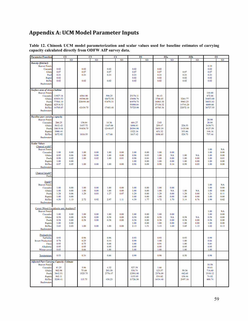
59

Appendix A: UCM Model Parameter Inputs Table 12. Chinook UCM model parameterization and scalar values used for baseline estimates of carrying capacity calculated directly from ODFW AIP survey data.

60

Table 8 continued. Chinook UCM model parameterization and scalar values

61

Table 13. Steelhead UCM model parameterization and scalar values used for baseline estimates of carrying capacity calculated directly from ODFW AIP survey data.

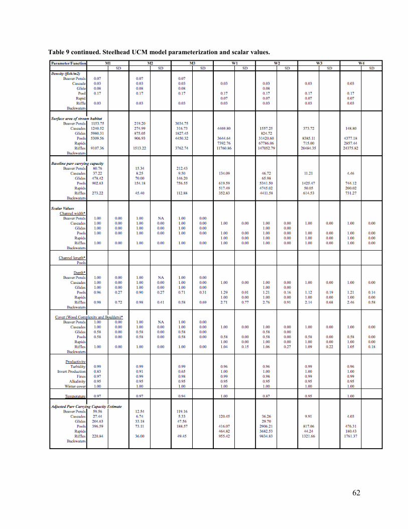
62

Table 9 continued. Steelhead UCM model parameterization and scalar values.

63

Appendix B: UCM-Flow DBHCP Scenario Output Black bars represent steelhead/redband trout and grey bars represent Chinook salmon

Crooked River

64

McKay Creek

65

Ochoco Creek

66

Deschutes River

67

Whychus Creek