Embed Size (px)
Citation preview
DBMS Storage Overview
1
Values
Records
Blocks
Files
Memory
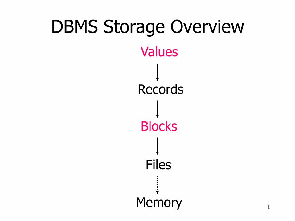
Record
§ Collection of related data items (called Fields)
§ Typically used to store one tuple § Example: Sells record consisting of
§ bar field § beer field § price field
2
Record Metadata
§ For fixed-length records, schema contains the following information: § Number of fields § Type of each field § Order in record
§ For variable-length records, every record contains this information in its header
3

Record Header
§ Reserved part at the beginning of a record
§ Typically contains: § Record type (which Schema?) § Record length (for skipping) § Time stamp (last access)
4
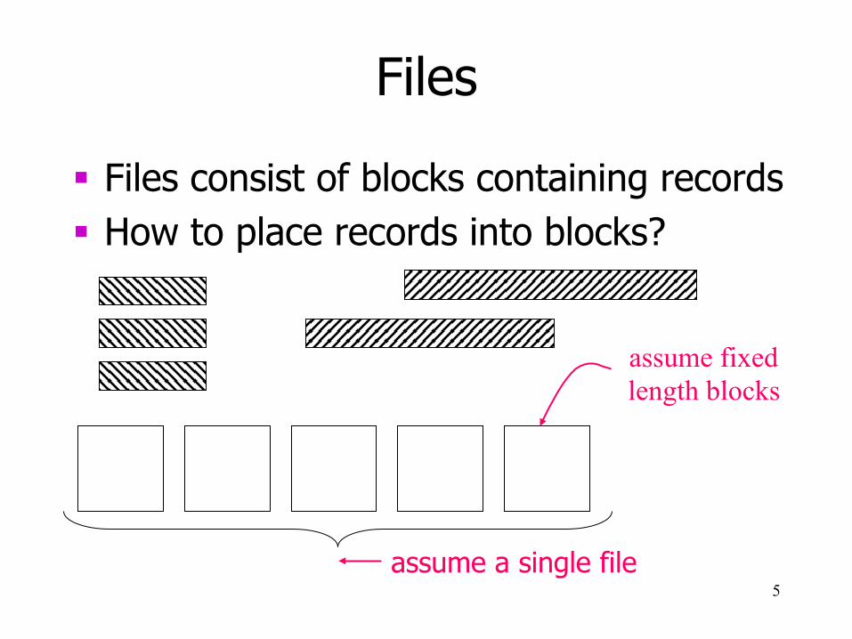
Files
§ Files consist of blocks containing records § How to place records into blocks?
5
assume fixed length blocks
assume a single file
Files
§ Options for storing records in blocks: 1. Separating records 2. Spanned vs. unspanned 3. Sequencing 4. Indirection
6
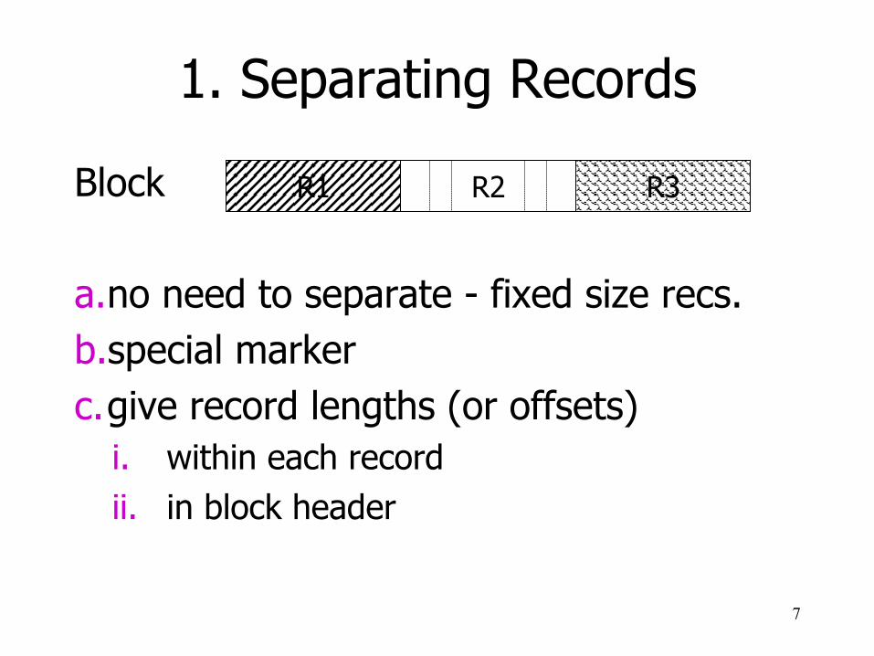
1. Separating Records
Block a. no need to separate - fixed size recs. b. special marker c. give record lengths (or offsets)
i. within each record ii. in block header
7
R2 R1 R3
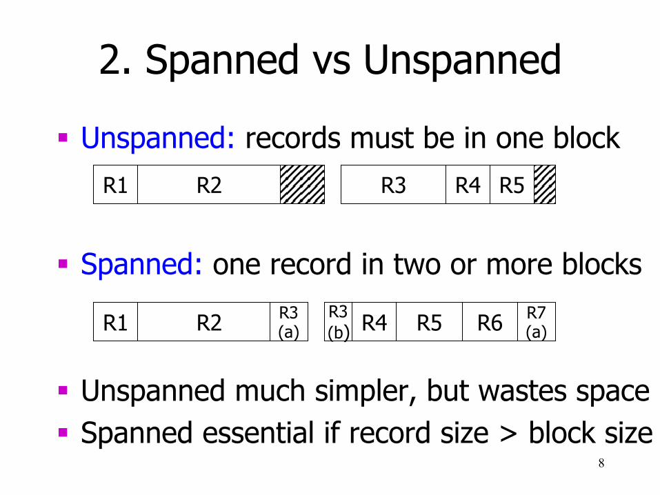
2. Spanned vs Unspanned
§ Unspanned: records must be in one block
§ Spanned: one record in two or more blocks
§ Unspanned much simpler, but wastes space § Spanned essential if record size > block size
8
R1 R2 R3 R4 R5
R1 R2 R3 (a)
R3 (b) R6 R5 R4 R7
(a)
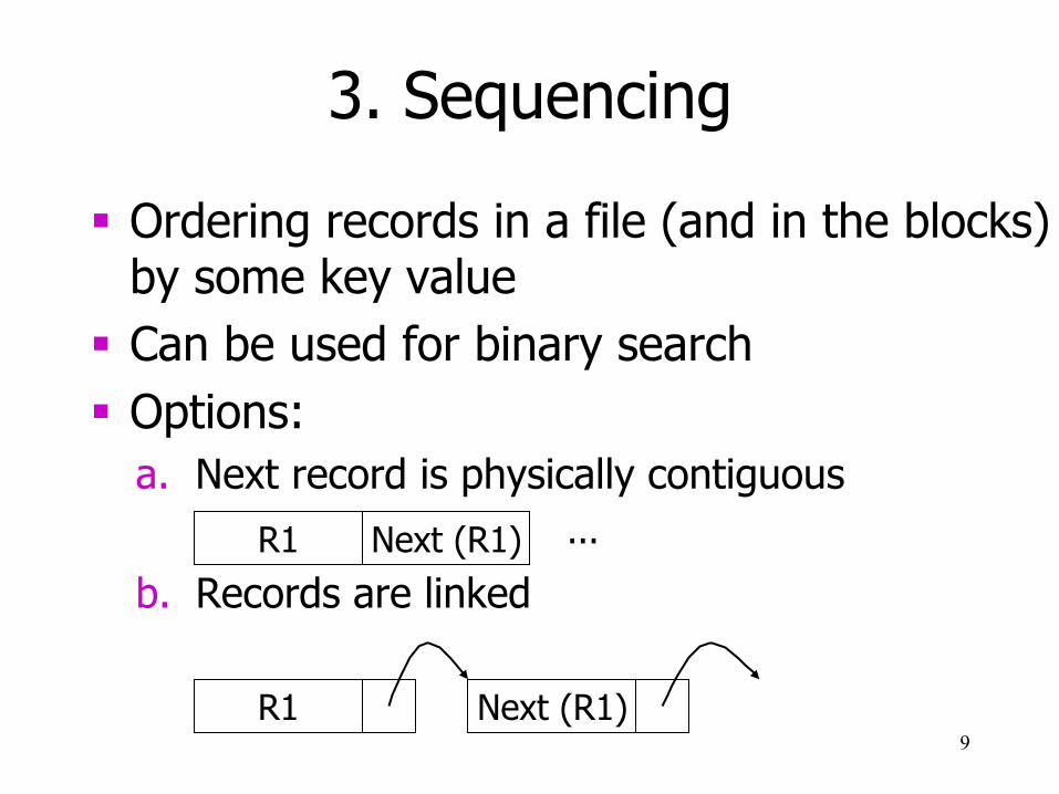
3. Sequencing
§ Ordering records in a file (and in the blocks) by some key value
§ Can be used for binary search § Options:
a. Next record is physically contiguous b. Records are linked
9
Next (R1) R1 ...
R1 Next (R1)
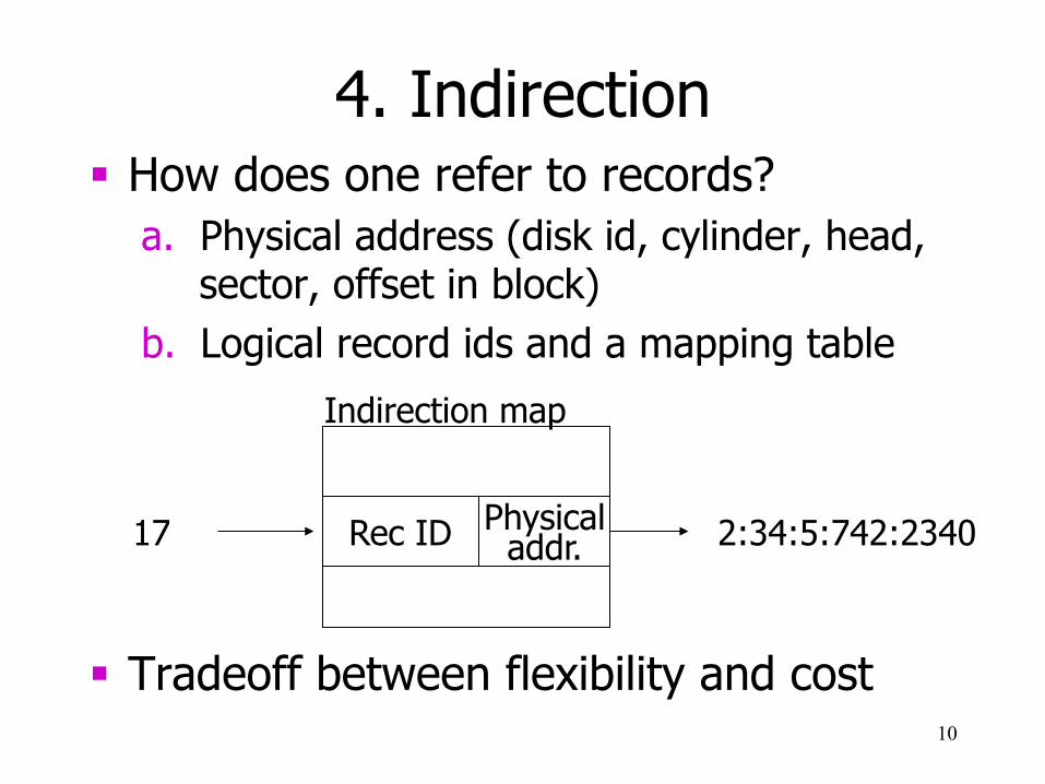
4. Indirection § How does one refer to records?
a. Physical address (disk id, cylinder, head, sector, offset in block)
b. Logical record ids and a mapping table
§ Tradeoff between flexibility and cost
10
Physical addr. Rec ID
Indirection map
17 2:34:5:742:2340
Modification of Records
How to handle the following operations on the record level? 1. Insertion 2. Deletion 3. Update
11
1. Insertion
§ Easy case: records not in sequence § Insert new record at end of file § If records are fixed-length, insert new
record in deleted slot
§ Difficult case: records are sorted § Find position and slide following records § If records are sequenced by linking, insert
overflow blocks
12
2. Deletion
a. Immediately reclaim space by shifting other records or removing overflows
b. Mark deleted and list as free for re-use § Tradeoffs:
§ How expensive is immediate reclaim? § How much space is wasted?
13
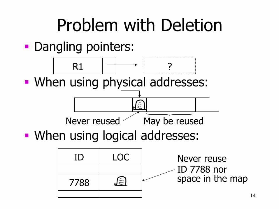
Problem with Deletion § Dangling pointers:
§ When using physical addresses:
§ When using logical addresses:
14
R1 ?
Never reused May be reused
ID LOC
7788
Never reuse ID 7788 nor space in the map

3. Update
§ If records are fixed-length and the order is not affected: § Fetch the record, modify it, write it back
§ Otherwise: § Delete the old record § Insert the new record overwriting the
tombstones from the deletion
15
Pointer Swizzling
§ Swizzling = replacement of physical addresses by memory addresses when loading blocks into memory
§ Automatic Swizzling: swizzle all addresses when loading a block (need to swizzle all pointer from and to the block)
§ Swizzling on Demand: use addresses which are invalid as memory addresses
16

Data Organizaton
§ There are millions of ways to organize the data on disk
§ Flexibility Space Utilization
Complexity Performance
17
Summary 9
More things you should know: § Memory Hierarchy § Storage on harddisks § Values, Records, Blocks, Files § Storing and modifying records
18

Index Structures
19
Finding Records
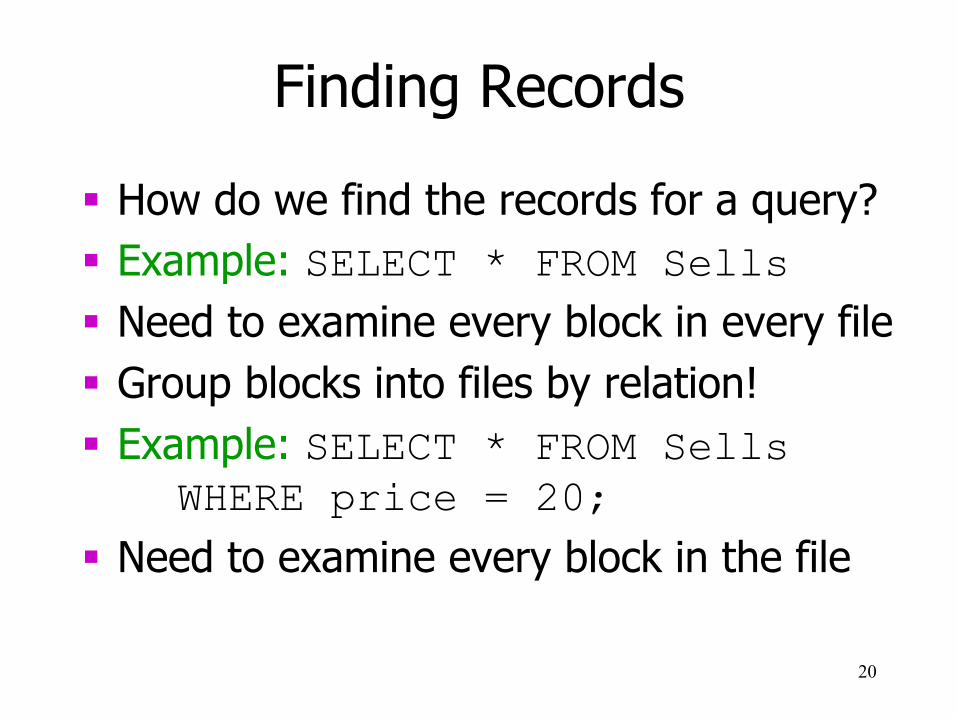
§ How do we find the records for a query? § Example: SELECT * FROM Sells § Need to examine every block in every file § Group blocks into files by relation! § Example: SELECT * FROM Sells
WHERE price = 20; § Need to examine every block in the file
20
Finding Records
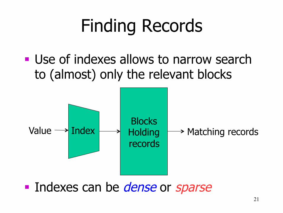
§ Use of indexes allows to narrow search to (almost) only the relevant blocks
21
Index Blocks Holding records
Value Matching records
§ Indexes can be dense or sparse
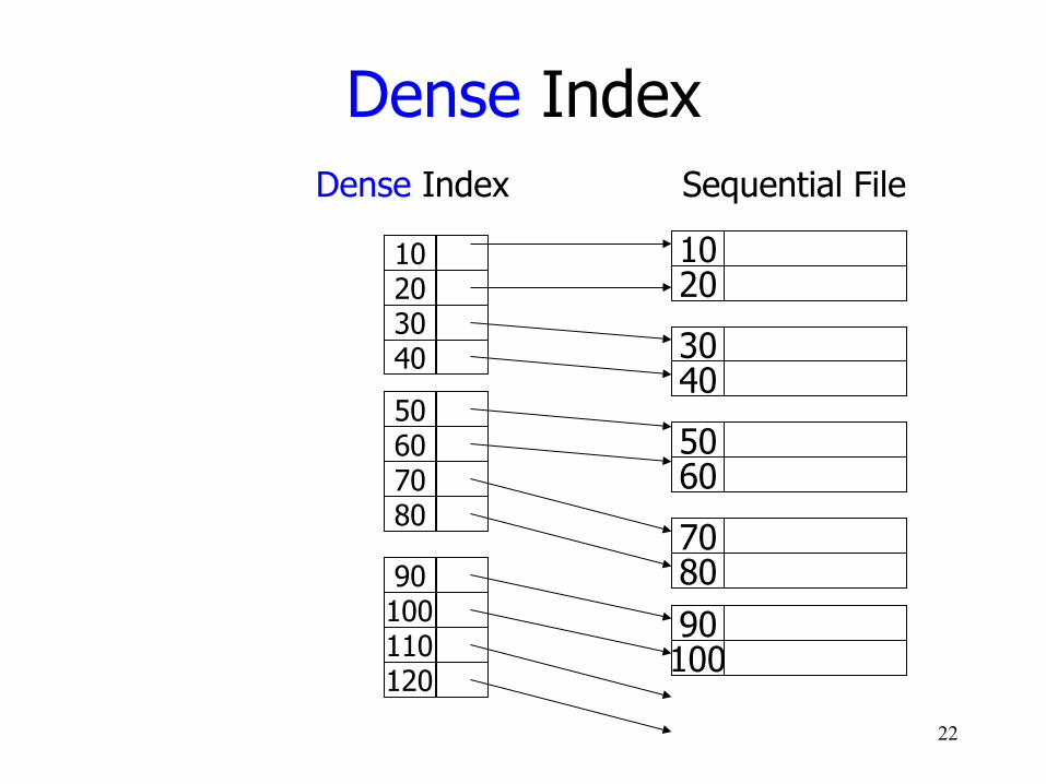
Dense Index
22
Sequential File
20 10
40 30
60 50
80 70
100 90
Dense Index
10 20 30 40
50 60 70 80
90 100 110 120

Sparse Index
23
Sequential File
20 10
40 30
60 50
80 70
100 90
Sparse Index
10 30 50 70
90 110 130 150
170 190 210 230
2nd level
10 90 170 250
330 410 490 570

40 30
§ Delete 40
Deletion from Sparse Index
24
20 10
60 50
80 70
10 30 50 70
90
110 130 150
40 30 30
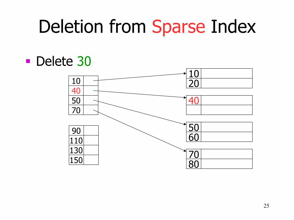
§ Delete 30
Deletion from Sparse Index
25
20 10
60 50
80 70
10 30 50 70
90
110 130 150
40 30 40 30 40 40
10 40 50 70
90
110 130 150
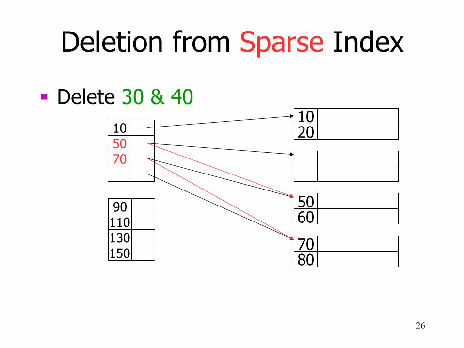
§ Delete 30 & 40
Deletion from Sparse Index
26
20 10
60 50
80 70
10 30 50 70
90
110 130 150
40 30 40 30
10 50 70
90
110 130 150
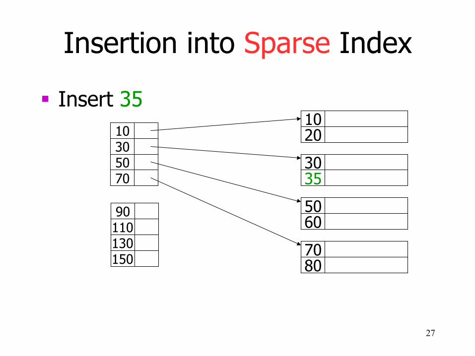
§ Insert 35
Insertion into Sparse Index
27
20 10
60 50
80 70
10 30 50 70
90
110 130 150
30 35 30
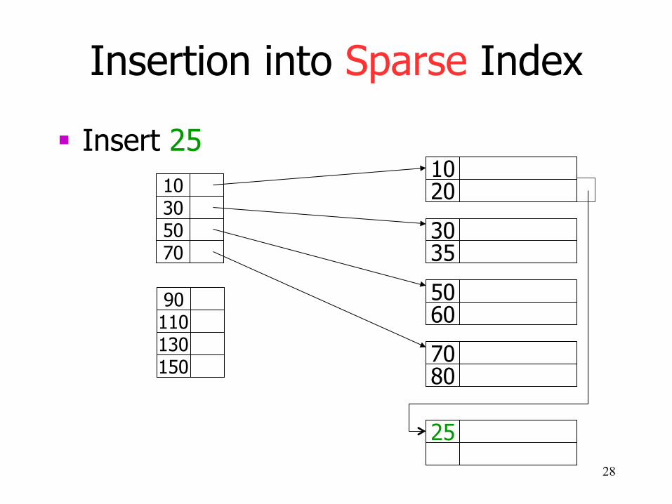
§ Insert 25
Insertion into Sparse Index
28
20 10
60 50
80 70
10 30 50 70
90
110 130 150
35 30
25
Sparse vs Dense
§ Sparse uses less index space per record (can keep more of index in memory)
§ Sparse allows multi-level indexes § Dense can tell if record exists without
accessing it § Dense needed for secondary indexes § Primary index = order of records in storage § Secondary index = impose different order
29
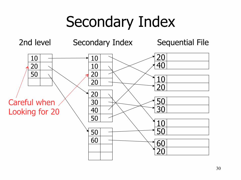
Secondary Index
30
Sequential File
40 20
20 10
30 50
50 10
20 60
Secondary Index
10 10 20 20
20 30 40 50
50 60
2nd level
10 20 50
Careful when Looking for 20

Secondary Index
31
Sequential File
40 20
20 10
30 50
50 10
20 60
Secondary Index
10 20 30 40
50 60
2nd level
10 50
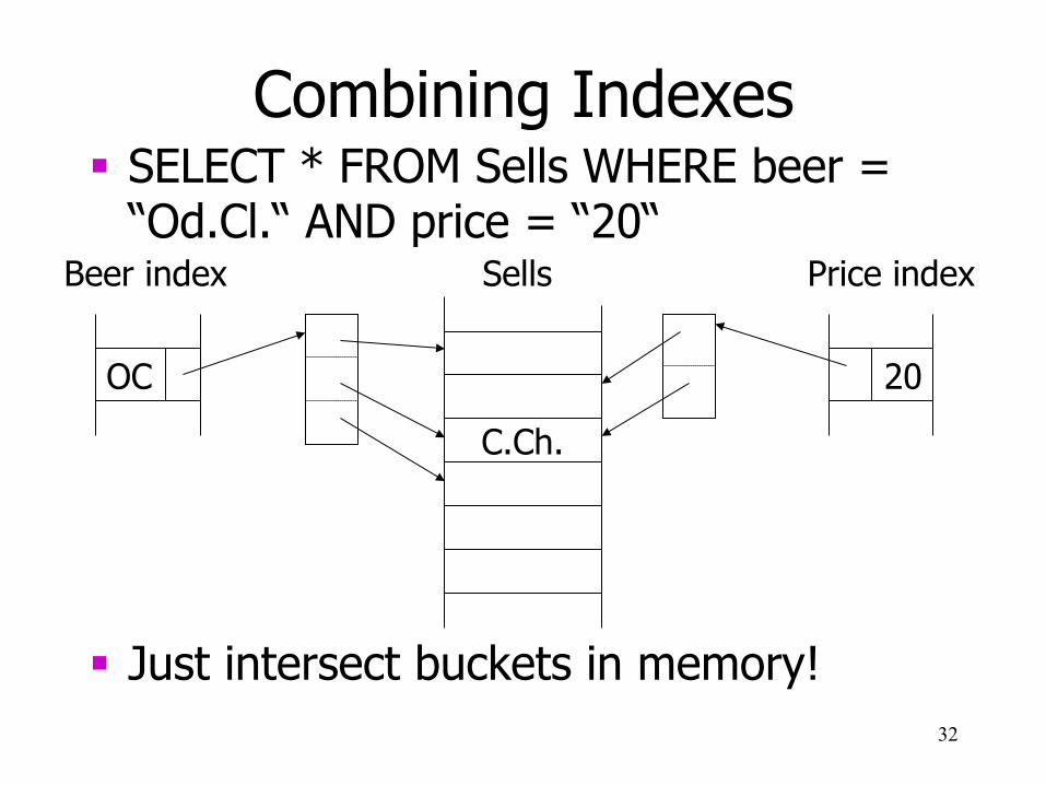
Combining Indexes
§ Just intersect buckets in memory! 32
Beer index Sells Price index
OC 20
§ SELECT * FROM Sells WHERE beer = “Od.Cl.“ AND price = “20“
C.Ch.
Conventional Indexes
§ Sparse, Dense, Multi-level, ... § Advantages:
§ Simple § Sequential index is good for scans
§ Disadvantage: § Inserts expensive § Lose sequentiality and balance
33
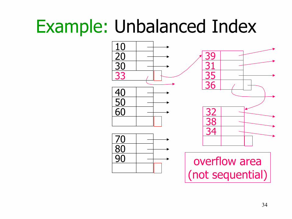
Example: Unbalanced Index
34
10 20 30
40 50 60
70 80 90
33
39 31 35 36
32 38 34
overflow area (not sequential)
B+Trees
35
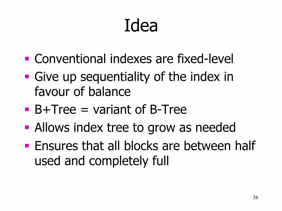
Idea
§ Conventional indexes are fixed-level § Give up sequentiality of the index in
favour of balance § B+Tree = variant of B-Tree § Allows index tree to grow as needed § Ensures that all blocks are between half
used and completely full
36

Characteristics
§ Parameter n determines number of keys and pointers per node
§ Key size 4 and pointer size 8 allows for maximal n = 340 (4n + 8(n+1) < 4096)
§ Leafs contain at least n/2 key-pointer pairs to records and a pointer to the next leaf
§ Interior nodes contain at least (n-1)/2 keys and at least n/2 pointers to other nodes
§ No restrictions for the root node 37

Example: B+Tree (n=3)
38
3 6 9 23 31 37 11 15 17 64 85 42 57
64 11 23
42
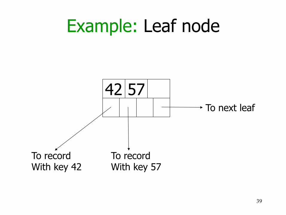
Example: Leaf node
39
42 57
To record With key 42
To record With key 57
To next leaf
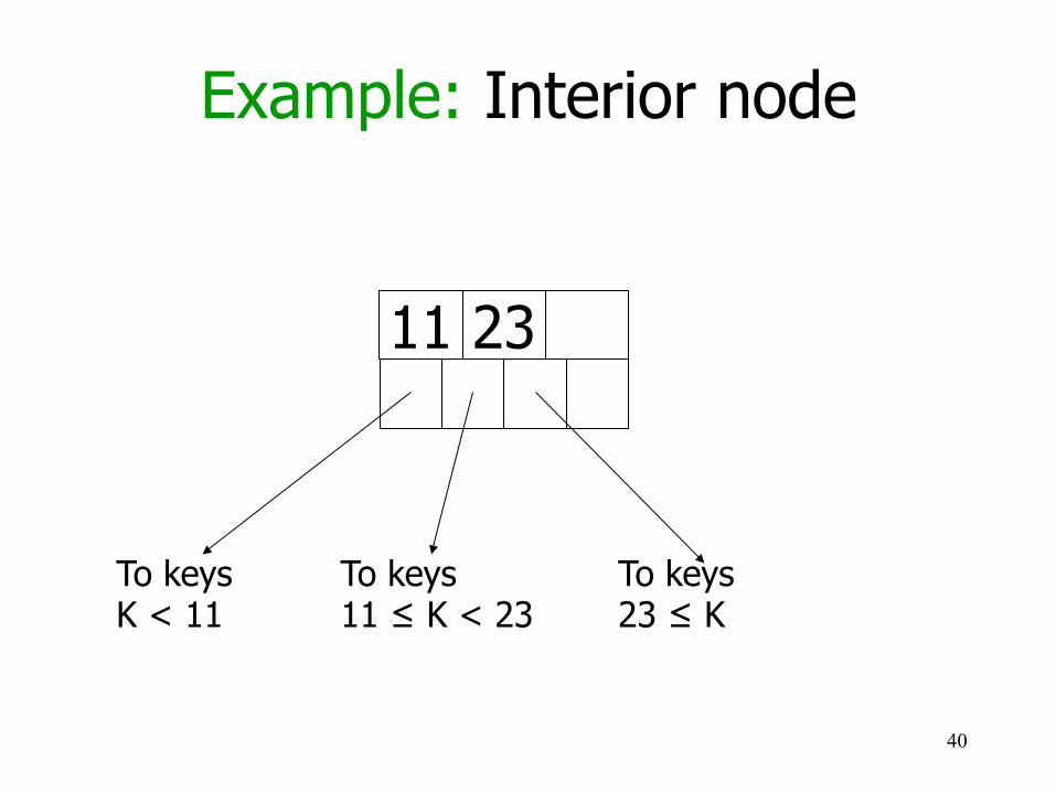
Example: Interior node
40
To keys K < 11
To keys 11 ≤ K < 23
11 23
To keys 23 ≤ K
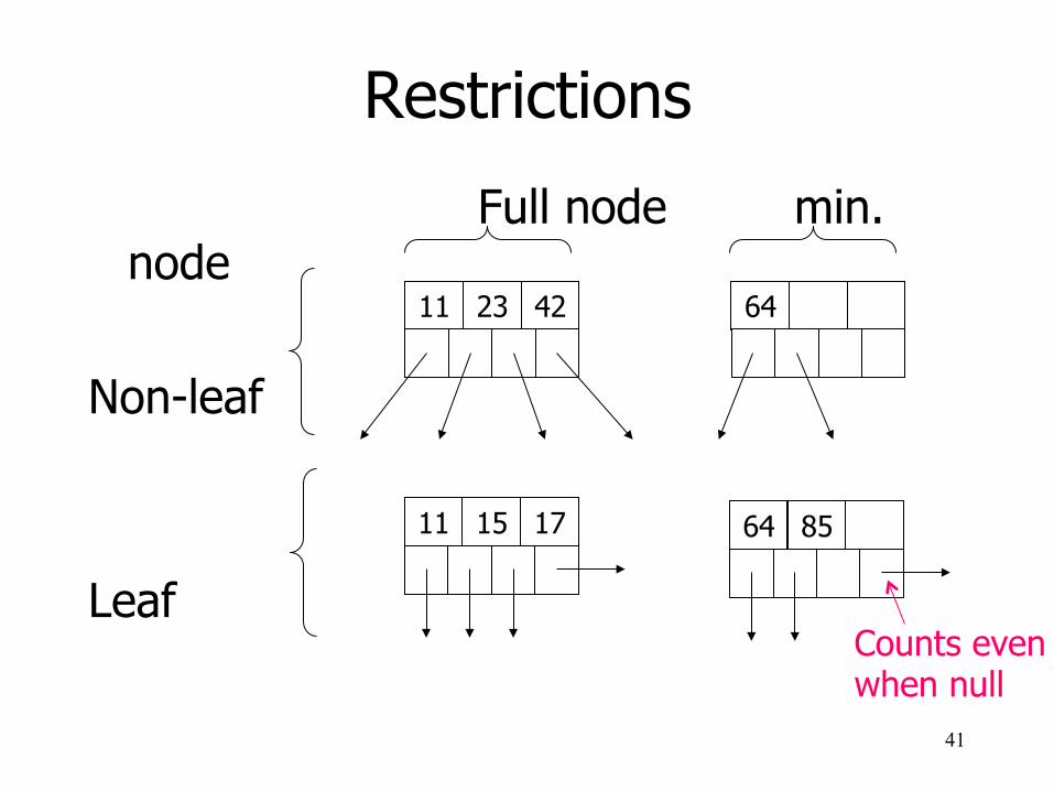
Restrictions
41
Full node min. node
Non-leaf Leaf
11 23 42 64
11 15 17 64 85
Counts even when null
Insertion
§ If there is place in the appropriate leaf, just insert it there
§ Otherwise: § Split the leaf in two and divide the keys § Insert the smallest value reachable through
the right node into the parent node § Recurse until there is enough room
§ Special case: Splitting the root results in a new root
42
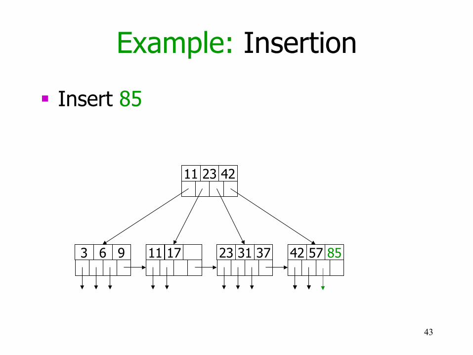
Example: Insertion
§ Insert 85
43
3 6 9 11 17 23 31 37 42 57
11 23 42
42 57 85
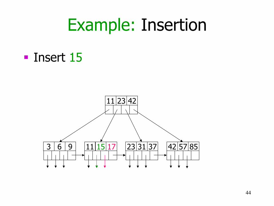
Example: Insertion
§ Insert 15
44
3 6 9 11 17 23 31 37
11 23 42
42 57 85 11 15 17
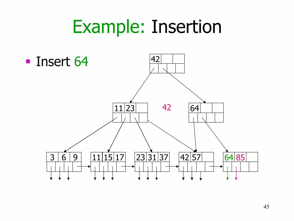
Example: Insertion
§ Insert 64
45
3 6 9 23 31 37
11 23 42
42 57 85 11 15 17 64 85 42 57
64 11 23
42
42

Deletion
§ If there are enough keys left in the appropriate leaf, just delete the key
§ Otherwise: § If there is a direct sibling with more than
minimum key, steal one! § If not, join the node with a direct sibling and
delete the smallest value reachable through the former right sibling from its parent
§ Special case: If the root contains only one pointer after deletion, delete it 46
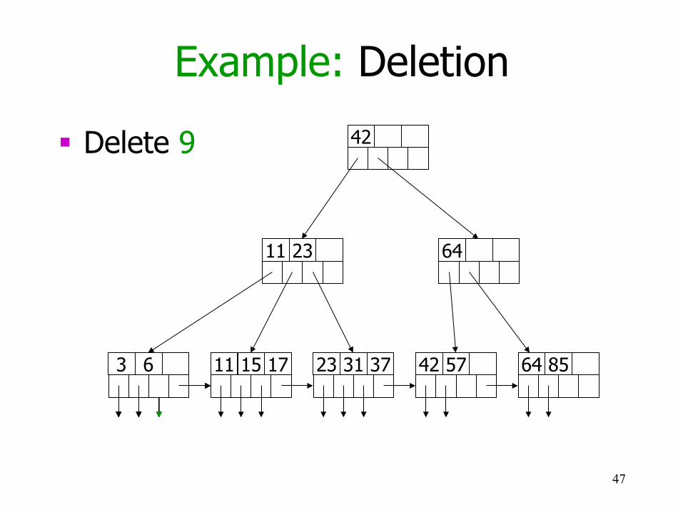
Example: Deletion
§ Delete 9
47
3 6 9 23 31 37 11 15 17 64 85 42 57
64 11 23
42
3 6 9 3 6
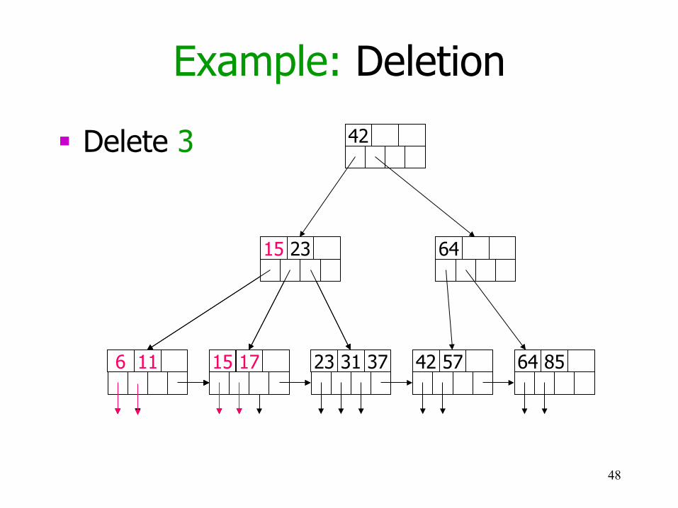
Example: Deletion
§ Delete 3
48
3 6 23 31 37 11 15 17 64 85 42 57
64 11 23
42
3 6 6 6 11 15 17
15 23
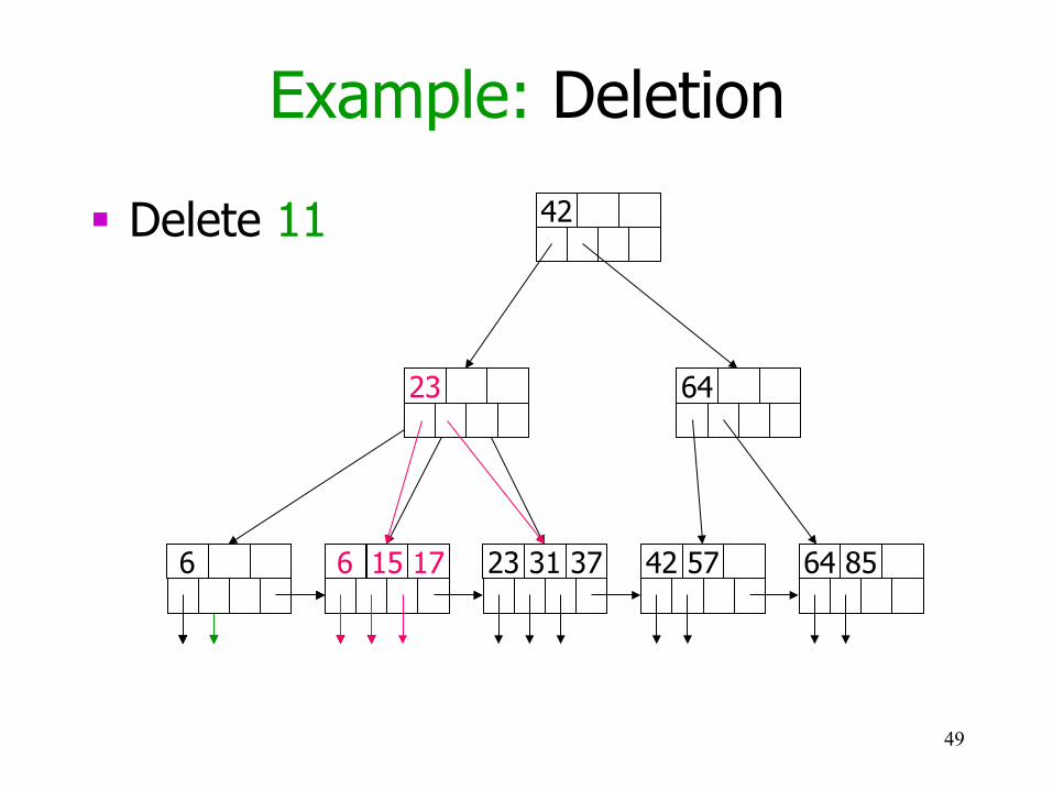
Example: Deletion
§ Delete 11
49
6 11 23 31 37 15 17 64 85 42 57
64 15 23
42
6 11 6 6 15 17
23
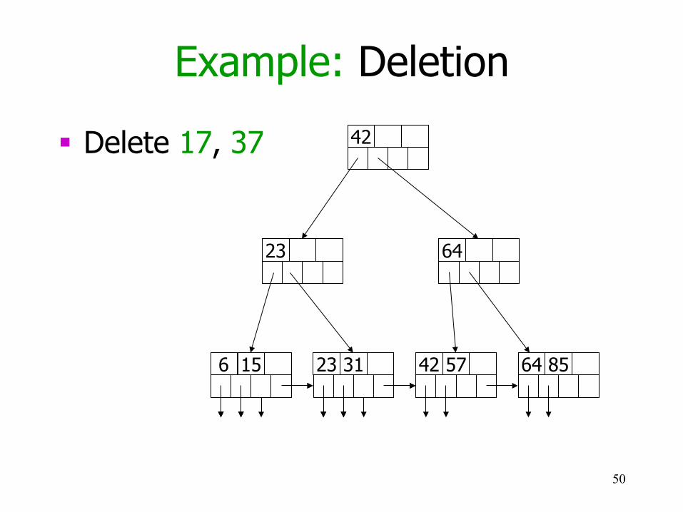
Example: Deletion
§ Delete 17, 37
50
23 31 37 64 85 42 57
64
42
6 15 17
23
6 15 23 31
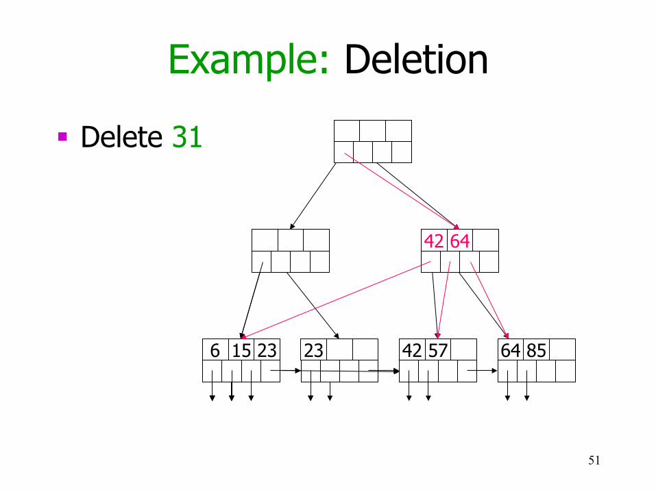
Example: Deletion
§ Delete 31
51
64 85 42 57
64
42
23
6 15 23 31 23 6 15 23 6 15 23
42 64
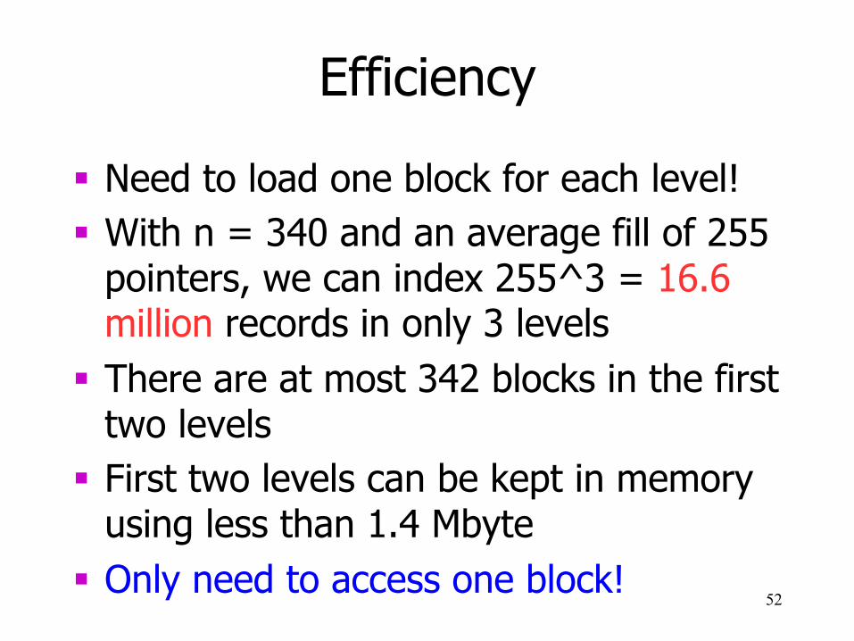
Efficiency
§ Need to load one block for each level! § With n = 340 and an average fill of 255
pointers, we can index 255^3 = 16.6 million records in only 3 levels
§ There are at most 342 blocks in the first two levels
§ First two levels can be kept in memory using less than 1.4 Mbyte
§ Only need to access one block! 52

Range Queries
§ Queries often restrict an attribute to a range of values
§ Example: SELECT * FROM Sells WHERE price > 20;
§ Records are found efficiently by searching for value 20 and then traversing the leafs
§ Can also be used if there is both an upper and a lower limit
53
Summary 10
More things you should know: § Dense Index, Sparse Index § Multi-Level Indexes § Primary vs Secondary Index § Structure of B+Trees § Insertion and Deletion in B+Trees
54
Hash Tables
55
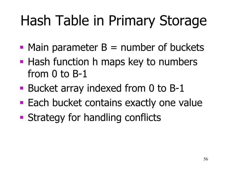
Hash Table in Primary Storage
§ Main parameter B = number of buckets § Hash function h maps key to numbers
from 0 to B-1 § Bucket array indexed from 0 to B-1 § Each bucket contains exactly one value § Strategy for handling conflicts
56
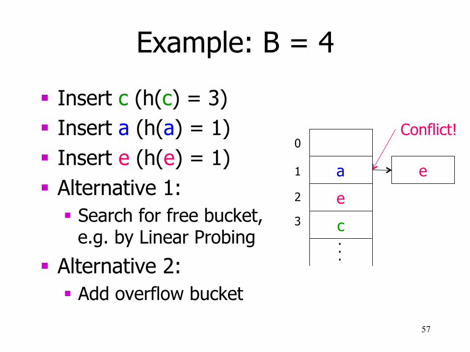
Example: B = 4
§ Insert c (h(c) = 3) § Insert a (h(a) = 1) § Insert e (h(e) = 1) § Alternative 1:
§ Search for free bucket, e.g. by Linear Probing
§ Alternative 2: § Add overflow bucket
57
. . .
0 1 2 3
Conflict!
a
c
e
e

Hash Function
§ Hash function should ensure hash values are equally distributed
§ For integer key K, take h(K) = K modulo B § For string key, add up the numeric values
of the characters and compute the remainder modulo B
§ For really good hash functions, see Donald Knuth, The Art of Computer Programming: Volume 3 – Sorting and Searching
58

Hash Table in Secondary Storage
§ Each bucket is a block containing f key-pointer pairs
§ Conflict resolution by probing potentially leads to a large number of I/Os
§ Thus, conflict resolution by adding overflow buckets
§ Need to ensure we can directly access bucket i given number i
59
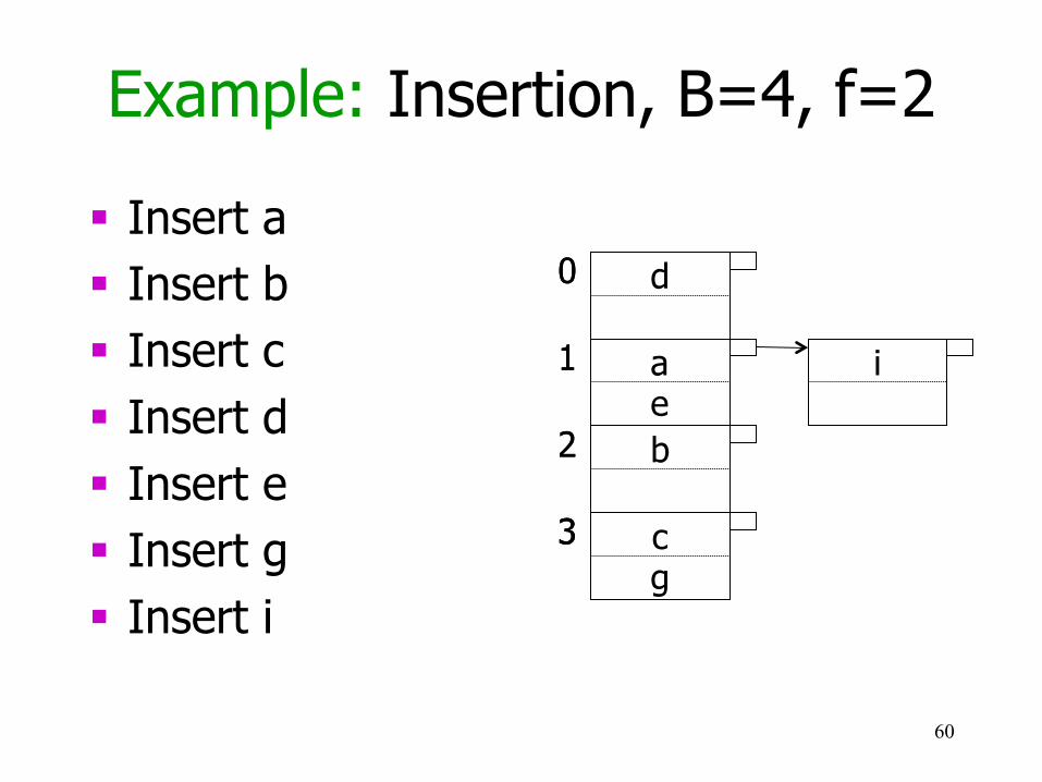
Example: Insertion, B=4, f=2
§ Insert a § Insert b § Insert c § Insert d § Insert e § Insert g § Insert i
60
0
1
2
3
a
1
b
2
c
3
d
0
a e
1
c g
3
i

Efficiency
§ Very efficient if buckets use only one block: one I/O per lookup
§ Space utilization is #keys in hash divided by total #keys that fit
§ Try to keep between 50% and 80%: § < 50% wastes space § > 80% significant number of overflows
61
Dynamic Hashing
§ How to grow and shrink hash tables? § Alternative 1:
§ Use overflows and reorganizations
§ Alternative 2: § Use dynamic hashing § Extensible Hash Tables § Linear Hash Tables
62
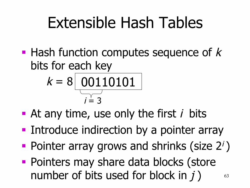
Extensible Hash Tables
§ Hash function computes sequence of k bits for each key k = 8
§ At any time, use only the first i bits § Introduce indirection by a pointer array § Pointer array grows and shrinks (size 2i ) § Pointers may share data blocks (store
number of bits used for block in j ) 63
00110101 i = 3

Example: k = 4, f = 2
64
i = 1
00
01
10
11
i = 2
1100
2
1001 1010
2
0001 0111
1
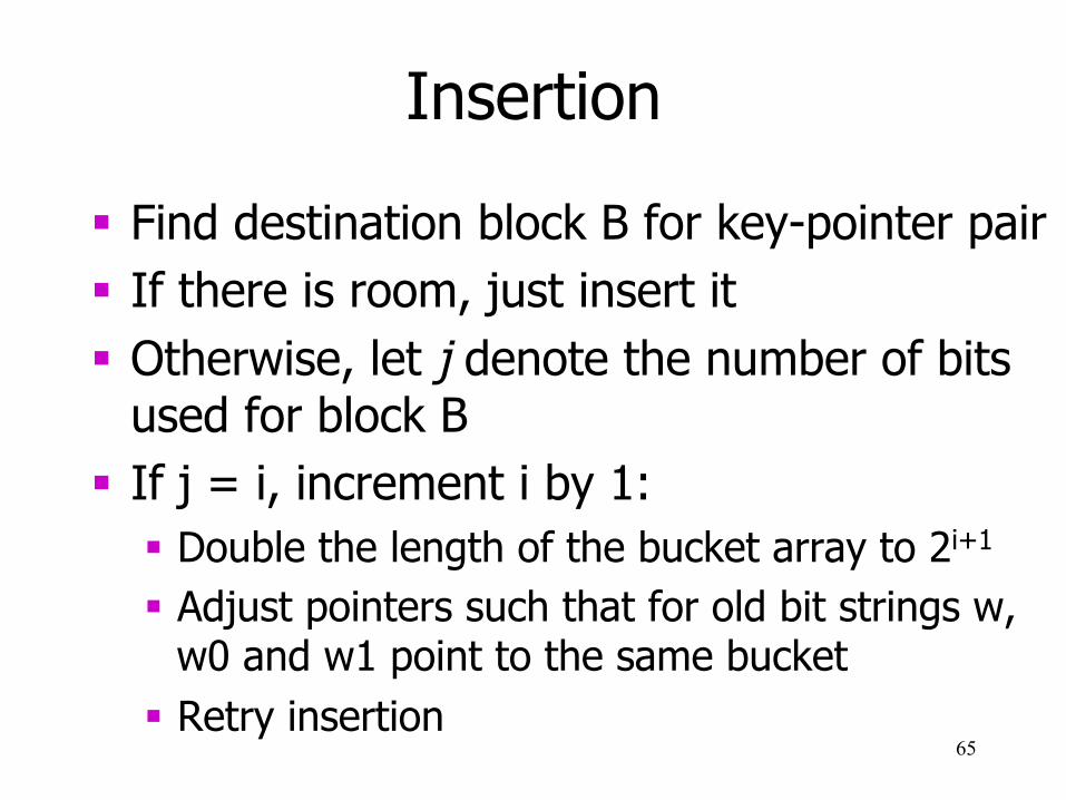
Insertion
§ Find destination block B for key-pointer pair § If there is room, just insert it § Otherwise, let j denote the number of bits
used for block B § If j = i, increment i by 1:
§ Double the length of the bucket array to 2i+1
§ Adjust pointers such that for old bit strings w, w0 and w1 point to the same bucket
§ Retry insertion
65
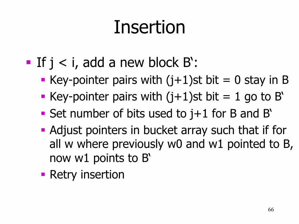
Insertion
§ If j < i, add a new block B‘: § Key-pointer pairs with (j+1)st bit = 0 stay in B § Key-pointer pairs with (j+1)st bit = 1 go to B‘ § Set number of bits used to j+1 for B and B‘ § Adjust pointers in bucket array such that if for
all w where previously w0 and w1 pointed to B, now w1 points to B‘
§ Retry insertion
66
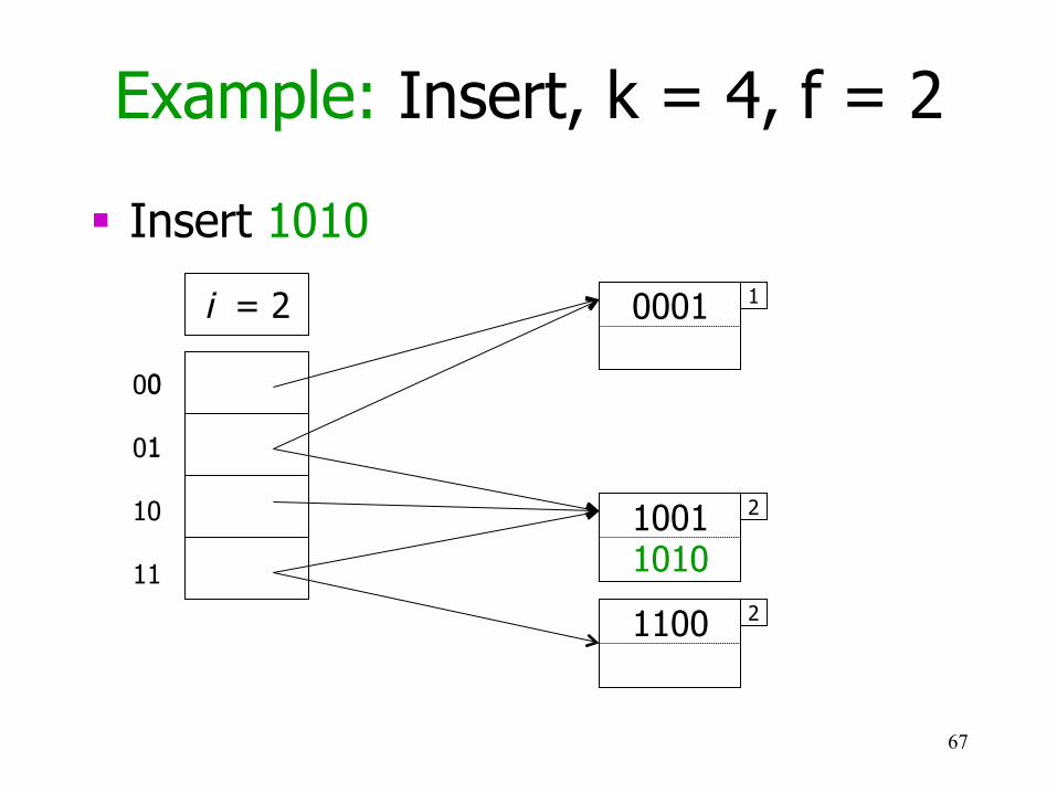
Example: Insert, k = 4, f = 2
§ Insert 1010
67
0001
1
1001 1100
1
0 1
i = 1
00
01
10
11
i = 2
1100
1 1100
2
1001
1 1001
2 1001 1010
2
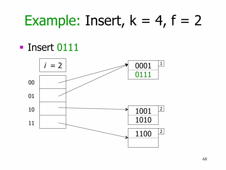
Example: Insert, k = 4, f = 2
§ Insert 0111
68
0001
1 i = 1
00
01
10
11
i = 2
1100
2
1001 1010
2
0001 0111
1

Example: Insert, k = 4, f = 2
§ Insert 0000
69
i = 1
00
01
10
11
i = 2
1100
2
1001 1010
2
0001 0111
1
0111
1
0001
1 0001
2
0111
2
0001 0000
2
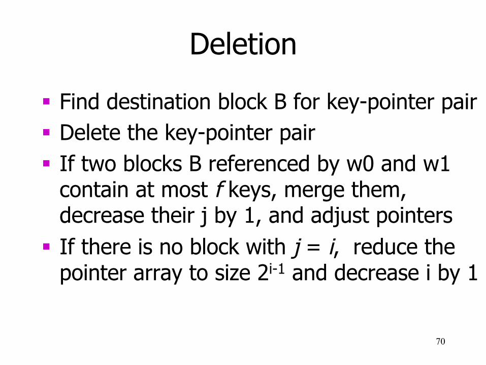
Deletion
§ Find destination block B for key-pointer pair § Delete the key-pointer pair § If two blocks B referenced by w0 and w1
contain at most f keys, merge them, decrease their j by 1, and adjust pointers
§ If there is no block with j = i, reduce the pointer array to size 2i-1 and decrease i by 1
70

Example: Delete, k = 4, f = 2
§ Delete 0000
71
i = 1
00
01
10
11
i = 2
1100
2
1001 1010
2
0001 0000
2
0111
2
0001
2 0001 0111
2 0001 0111
1
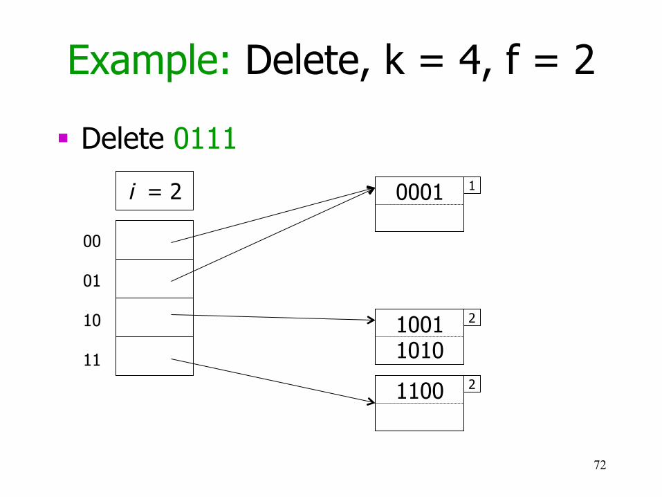
Example: Delete, k = 4, f = 2
§ Delete 0111
72
i = 1
00
01
10
11
i = 2
1100
2
1001 1010
2
0001 0111
1 0001
1
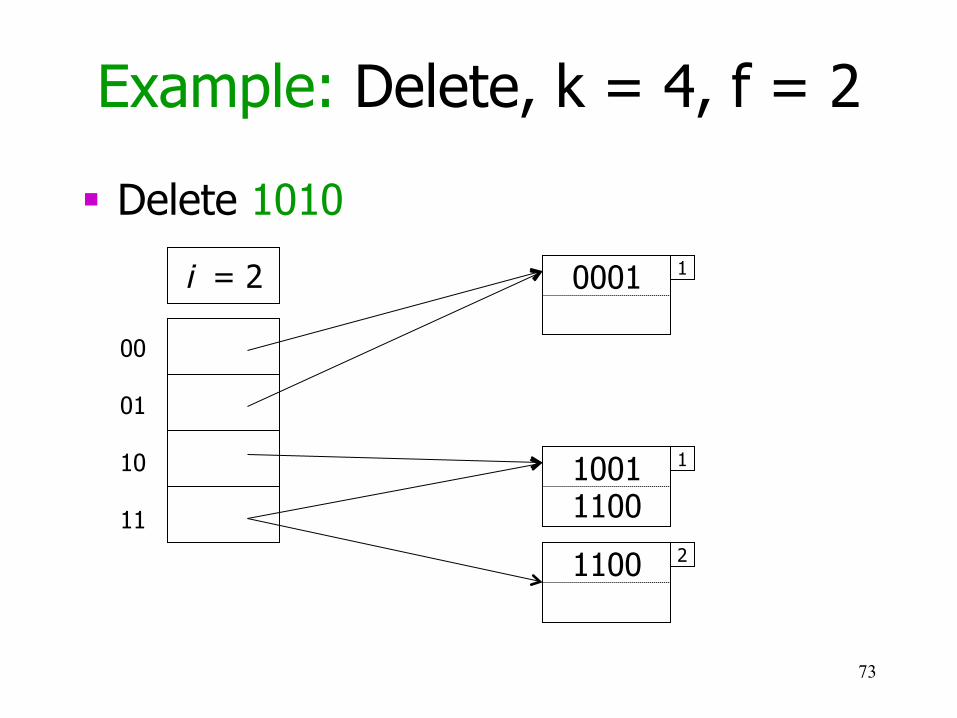
Example: Delete, k = 4, f = 2
§ Delete 1010
73
i = 1
00
01
10
11
i = 2
1100
2
1001 1010
2
0001
1
1001
2 1001 1100
2 1001 1100
1

Efficiency
§ As long as pointer array fits into memory and hash function behaves nicely, just need one I/O per lookup
§ Overflows can still happen if many key-pointer pairs hash to the same bit string
§ Solve by adding overflow blocks
74