1

DC Motor Speed: System Modeling (Lab 6)

System equations

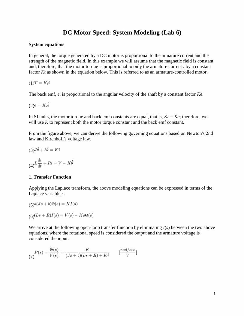
In general, the torque generated by a DC motor is proportional to the armature current and the

strength of the magnetic field. In this example we will assume that the magnetic field is constant

and, therefore, that the motor torque is proportional to only the armature current i by a constant

factor Kt as shown in the equation below. This is referred to as an armature-controlled motor.

(1)

The back emf, e, is proportional to the angular velocity of the shaft by a constant factor Ke.

(2)

In SI units, the motor torque and back emf constants are equal, that is, Kt = Ke; therefore, we

will use K to represent both the motor torque constant and the back emf constant.

From the figure above, we can derive the following governing equations based on Newton's 2nd

law and Kirchhoff's voltage law.

(3)

(4)

1. Transfer Function

Applying the Laplace transform, the above modeling equations can be expressed in terms of the

Laplace variable s.

(5)

(6)

We arrive at the following open-loop transfer function by eliminating I(s) between the two above

equations, where the rotational speed is considered the output and the armature voltage is

considered the input.

(7)

2

Physical setup

A common actuator in control systems is the DC motor. It directly provides rotary motion and,

coupled with wheels or drums and cables, can provide translational motion. The electric circuit

of the armature and the free-body diagram of the rotor are shown in the following figure:

For this example, we will assume that the input of the system is the voltage source (V) applied to

the motor's armature, while the output is the rotational speed of the shaft d(theta)/dt. The rotor

and shaft are assumed to be rigid. We further assume a viscous friction model, that is, the friction

torque is proportional to shaft angular velocity.

The physical parameters for our example are:

(J) moment of inertia of the rotor 0.01 kg.m^2

(b) motor viscous friction constant 0.1 N.m.s

(Ke) electromotive force constant 0.01 V/rad/sec

(Kt) motor torque constant 0.01 N.m/Amp

(R) electric resistance 1 Ohm

(L) electric inductance 0.5 H

In SI units, the motor torque and back emf constants are equal, that is, Kt = Ke; therefore, we

will use K to represent both the motor torque constant and the back emf constant.

Building the model with Simulink

This system will be modeled by summing the torques acting on the rotor inertia and integrating

the acceleration to give velocity. Also, Kirchoff's laws will be applied to the armature circuit.

First, we will model the integrals of the rotational acceleration and of the rate of change of the

armature current.

(3)

3

(4)

To build the simulation model, open Simulink and open a new model window. Then follow the

steps listed below.

Insert an Integrator block from the Simulink/Continuous library and draw lines to and

from its input and output terminals.

Label the input line "d2/dt2(theta)" and the output line "d/dt(theta)" as shown below. To

add such a label, double-click in the empty space just below the line.

Insert another Integrator block above the previous one and draw lines to and from its

input and output terminals.

Label the input line "d/dt(i)" and the output line "i".

Next, we will apply Newton's law and Kirchoff's law to the motor system to generate the

following equations:

(5)

(6)

The angular acceleration is equal to 1 / J multiplied by the sum of two terms (one positive, one

negative). Similarly, the derivative of current is equal to 1 / L multiplied by the sum of three

4

terms (one positive, two negative). Continuing to model these equations in Simulink, follow the

steps given below.

Insert two Gain blocks from the Simulink/Math Operations library, one attached to each

of the integrators.

Edit the Gain block corresponding to angular acceleration by double-clicking it and

changing its value to "1/J".

Change the label of this Gain block to "Inertia" by clicking on the word "Gain"

underneath the block.

Similarly, edit the other Gain's value to "1/L" and its label to "Inductance".

Insert two Add blocks from the Simulink/Math Operations library, one attached by a line

to each of the Gain blocks.

Edit the signs of the Add block corresponding to rotation to "+-" since one term is

positive and one is negative.

Edit the signs of the other Add block to "-+-" to represent the signs of the terms in the

electrical equation.

Now, we will add in the torques which are represented in the rotational equation. First, we will

add in the damping torque.

Insert a Gain block below the "Inertia" block. Next right-click on the block and select

Format > Flip Block from the resulting menu to flip the block from left to right. You

can also flip a selected block by holding down Ctrl-I.

Set the Gain value to "b" and rename this block to "Damping".

5

Tap a line (hold Ctrl while drawing or right-click on the line) off the rotational

Integrator's output and connect it to the input of the "Damping" block.

Draw a line from the "Damping" block output to the negative input of the rotational Add

block.

Next, we will add in the torque from the armature.

Insert a Gain block attached to the positive input of the rotational Add block with a line.

Edit its value to "K" to represent the motor constant and Label it "Kt".

Continue drawing the line leading from the current Integrator and connect it to the "Kt"

block.

Now, we will add in the voltage terms which are represented in the electrical equation. First, we

will add in the voltage drop across the armature resistance.

Insert a Gain block above the "Inductance" block and flip it from left to right.

Set the Gain value to "R" and rename this block to "Resistance".

Tap a line off the current Integrator's output and connect it to the input of the

"Resistance" block.

Draw a line from the "Resistance" block's output to the upper negative input of the

current equation Add block.

Next, we will add in the back emf from the motor.

6

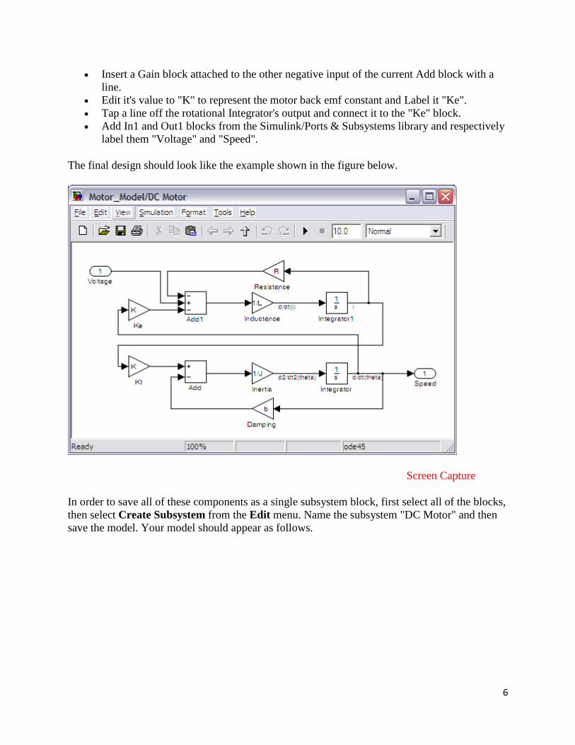
Insert a Gain block attached to the other negative input of the current Add block with a

line.

Edit it's value to "K" to represent the motor back emf constant and Label it "Ke".

Tap a line off the rotational Integrator's output and connect it to the "Ke" block.

Add In1 and Out1 blocks from the Simulink/Ports & Subsystems library and respectively

label them "Voltage" and "Speed".

The final design should look like the example shown in the figure below.

Screen Capture

In order to save all of these components as a single subsystem block, first select all of the blocks,

then select Create Subsystem from the Edit menu. Name the subsystem "DC Motor" and then

save the model. Your model should appear as follows.

7

We then need to identify the inputs and outputs of the model we wish to extract. First right-click

on the signal representing the Voltage input in the Simulink model. Then choose Linearization

> Input Point from the resulting menu. Similarly, right-click on the signal representing the

Speed output and select Linearization > Output Point from the resulting menu. The input and

output signals should now be identified on your model by arrow symbols as shown in the figure

below.

8

In order to perform the extraction, select from the menus at the top of the model window Tools >

Control Design > Linear Analysis. This will cause the Linear Analysis Tool to open. Within

the Linear Analysis Tool window, the Operating Point to be linearized about can remain the

default, Model Initial Condition. In order to perform the linearization, next click the

Linearize button identified by the green triangle. The result of this linearization is the linsys1

object which now appears in the Linear Analysis Workspace as shown below. Furthermore, the

open-loop step response of the linearized system was also generated automatically.

Screen Capture

9

Open-loop response

The open-loop step response can also be generated directly within Simulink, without extracting

any models to the MATLAB workspace. In order to simulate the step response, the details of the

simulation must first be set. This can be accomplished by selecting Configuration Parameters

from the Simulation menu. Within the resulting menu, define the length for which the

simulation is to run in the Stop time field. We will enter "3" since 3 seconds will be long enough

for the step response to reach steady state. Within this window you can also specify various

aspects of the numerical solver, but we will just use the default values for this example.

Next we need to add an input signal and a means for displaying the output of our simulation.

This is done by doing the following:

Remove the In1 and Out1 blocks.

Insert a Step block from the Simulink/Sources library and connect it with a line to the

Voltage input of the motor subsystem.

To view the Speed output, insert a Scope from the Simulink/Sinks library and connect it

to the Speed output of the motor subsystem.

To provide a appropriate unit step input at t=0, double-click the Step block and set the

Step time to "0".

The final model should appear as shown in the following figure.

10

Then run the simulation (press Ctrl-T or select Start from the Simulation menu). When the

simulation is finished, double-click on the scope and hit its autoscale button. You should see the

following output.

Screen Capture

Adding a lag controller

A lag compensator is one type of controller known to be able to reduce steady-state error.

However, we must be careful in our design to not increase the settling time too much. Let's first

try adding a lag compensator of the form given below.

(4)

We can use the SISO Design Tool to design our lag compensator. To make the SISO Design

Tool have a compensator parameterization corresponding to the one shown above, click on the

Edit menu at the top of the Control and Estimation Tools Manager window and choose SISO

Tool Preferences. Then From the Options tab, select a Zero/pole/gain parameterization as

shown below.

11

You can then add the lag compensator from under the Compensator Editor tab of the Control

and Estimation Tools Manager window. Specifically, right-click in the Dynamics section of

the window and select Add Pole/Zero > Lag. Then enter the Real Zero and Real Pole locations

as shown in the following figure.

12

Note that the phase lag contributed by the compensator and the frequency where it is located are

updated to match the pole and zero locations chosen.

Closed-loop response with lag compensator

A lag compensator was designed with the following transfer function.

(2)

We will put the lag compensator in series with the motor subsystem and will feed back the

motor's speed for comparison to a desired reference.

More specifically, follow the steps given below:

Remove the Input and Output ports of the model.

Insert a Sum block from the Simulink/Math Operations library. Then double-click on the

block and enter "|+-" for its List of signs where the symbol "|" serves as a spacer between

ports of the block.

Insert a Transfer Function block from the Simulink/Continuous library. Then double-

click on the block and edit the Numerator coefficients field to "[44 44]" and the

Denominator coefficients field to "[1 0.01]".

Insert a Step block from the Simulink/Sources library. Then double-click on the block

and set the Step time to "0".

Insert a Scope block from the Simulink/Sinks library.

Then connect and label the components as shown in the following figure

13

Then run the simulation (press Ctrl-T or select Start from the Simulation menu). When the

simulation is finished, double-click on the scope and hit its auto-scale button. You should see the

following output.

Screen Capture

Closed-loop response with lead compensator

We have shown in the above and in other pages of this example that the lag compensator we

have designed meets all of the given design requirements. Instead of a lag compensator, we

could have also designed a lead compensator to meet the given requirements. More specifically,

we could have designed a lead compensator to achieve a similar DC gain and phase margin to

that achieved by the lag compensator, but with a larger gain crossover frequency. The DC gains

and phase margins are similar indicate that the responses under lag and lead control would have

similar amounts of error in steady state and similar amounts of overshoot. The difference in

response would come in that the larger gain crossover frequency provided by the lead

compensator would make the system response faster than with the lag compensator. We will

specifically use the following lead compensator.

(3)

To see the precise effect of the lead compensator as compared to our lag compensator, let's

modify our Simulink model from above as follows:

Disconnect the Step block and Scope block from the rest of the model.

Copy the blocks forming the closed-loop of the model: the Sum block, the Transfer

Function block, and the DC Motor subsystem. Then paste a copy of this loop below the

original blocks.

Double-click on the Transfer Function block and edit the Numerator coefficients field to

"[160000 5.6e6]" and the Denominator coefficients field to "[1 1035]".

14

Insert a Mux block from the Simulink\Signal Routing library and connect the outputs of

the two Motor subsystem blocks to the inputs of the Mux and connect the output of the

Mux to the Scope.

Connect the Step block to the Sum block of the original feedback system. Then branch

off from this line and connect it to the Sum block of the lead compensated system as well.

The Mux block serves to bundle the two signals into a single line, this way the Scope will plot

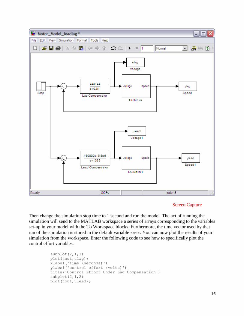
both speed signals on the same set of axes. When you are done, your model should appear as

follows.

Screen Capture

Running the simulation and observing the output produced by the scope, you will see that both

responses have a steady-state error that approaches zero. Zooming in on the graphs you can

generate a figure like the one shown below. Comparing the two graphs, the purple response

belonging to the lead compensated system has a much smaller settle time and slightly larger, but

similar, overshoot as compared to the yellow response produced by the lag compensated system.

15

Screen Capture

It is generally preferred that a system respond to a command quickly. Why then might we prefer

to use the lag compensator even though it is slower than the lead compensator? The advantage of

the lag compensator in this case is that by responding more slowly it requires less control effort

than the lead compensator. Less control effort means that less power is consumed and that the

various components can be sized smaller since they do not have to supply as much energy or

withstand the higher voltages and current required of the lead compensator.

We will now modify our simulation to explicitly observe the control effort requirements of our

two feedback systems. We will do this by sending our various signals to the workspace for

plotting and further manipulation if desired. Specifically, delete the Scope and Mux blocks from

your Simulink model. Then insert four To Workspace blocks from the Simulink\Sinks library.

Double-click on each of the blocks and change their Save format from Structure to Array.

Also provide a Variable name within each block that will make sense to you. You can then

connect the blocks to the existing model and label them as shown below.

16

Screen Capture

Then change the simulation stop time to 1 second and run the model. The act of running the

simulation will send to the MATLAB workspace a series of arrays corresponding to the variables

set-up in your model with the To Workspace blocks. Furthermore, the time vector used by that

run of the simulation is stored in the default variable tout. You can now plot the results of your

simulation from the workspace. Enter the following code to see how to specifically plot the

control effort variables.

subplot(2,1,1)

plot(tout,ulag);

xlabel('time (seconds)')

ylabel('control effort (volts)')

title('Control Effort Under Lag Compensation')

subplot(2,1,2)

plot(tout,ulead);

17

xlabel('time (seconds)')

ylabel('control effort (volts)')

title('Control Effort Under Lead Compensation')

Screen Capture

Examination of the above shows that the control effort required by the lead compensator is above

150,000 Volts, which is well above anything that could be supplied or withstood by a typical DC

motor. This exemplifies the tradeoff inherent between achieving small tracking error and keeping

the amount of control effort required small.