energies

Article

DC/DC Boost Converter–Inverter as Driver for a DCMotor: Modeling and Experimental Verification

Víctor Hugo García-Rodríguez 1,2 , Ramón Silva-Ortigoza 1,∗ ,Eduardo Hernández-Márquez 1,3 , José Rafael García-Sánchez 1 and Hind Taud 1

1 Área de Mecatrónica, Centro de Innovación y Desarrollo Tecnológico en Cómputo, Instituto PolitécnicoNacional, Ciudad de México 07700, México; vhgarcia@sandunga.unistmo.edu.mx (V.H.G.-R.);eduardohm_1@hotmail.com (E.H.-M.); jrgs_ipn@hotmail.com (J.R.G.-S.); htaud@ipn.mx (H.T.)

2 Departamento de Ingeniería en Diseño, Universidad del Istmo, Oaxaca 70760, México3 Departamento de Mecatrónica, Instituto Tecnológico Superior de Poza Rica, Veracruz 93230, México* Correspondence: rsilvao@ipn.mx; Tel.: +52-55-5729-6000 (ext. 52530)

Received: 29 June 2018; Accepted: 27 July 2018; Published: 7 August 2018

Abstract: In this paper, the modeling and the experimental verification of the “bidirectionalDC/DC boost converter–DC motor” system are presented. By using circuit theory along withthe model of a DC motor, the mathematical model of the system is derived. This model wasexperimentally tested under time-varying duty cycles obtained via the system differential flatnessproperty. The experimental verification was carried out using Matlab-Simulink and a DS1104 boardin a built prototype of the system.

Keywords: DC/DC boost converter; inverter; DC motor; modeling; experimental verification;bidirectional angular velocity; differential flatness

1. Introduction

Nowadays, DC/DC power electronic converters are used in several applications [1–6].Such applications include, among others, renewable energies, aircraft, electric vehicles, robots,and telecommunications. If some of these applications require the generation of movement, thenelectric motors are generally used. In this direction, driving DC motors is achieved by means ofPWM. However, PWM switching induces abrupt variations in DC motor voltage and current [7].These variations can be reduced when the DC motor is fed via DC/DC converters [7,8]. DC/DCconverters change an input DC voltage level to a higher or lower output voltage level with a smallcurrent ripple. This latter is an intrinsic feature of a power converter because of the capacitor andthe inductor composing it. In this paper, a cascaded connection between a DC/DC boost converter,an inverter, and a DC motor is proposed, achieving a bidirectional rotation of the motor shaft.

The state of the art related to works dealing with a boost converter coupled with a DC motorfor driving unidirectional angular velocity is as follows. Lyshevski [8] developed the mathematicalmodels of the buck, boost, and Cuk converters that feed a DC motor. Linares-Flores et al. [9] reportedthe design of a passivity-based tracking control that is robust to torque variations. Alexandridis andKonstantopoulos [10] presented a nonlinear PI control that does not require current sensors for solvingthe regulation task, and the same authors developed a regulation nonlinear control that providesa closed-loop passive system that is robust to load variations [11]. Additional works in which differenttopologies of DC/DC power converters have been used in combination with a DC motor are thefollowing: [12–25] for the buck converter, [26,27] for the buck–boost converter, and [28] for the SEPICand Cuk converters. Because of the operation principle of the DC/DC converters, works reportedin [7–20,26–28] were only focused on driving the motor shaft in an unidirectional fashion for solvingboth the regulation and tracking problems.

Energies 2018, 11, 2044; doi:10.3390/en11082044 www.mdpi.com/journal/energies

Energies 2018, 11, 2044 2 of 15

On the other hand, works in which the bidirectional rotation of the motor shaft wasaddressed, when a DC/DC converter and an inverter were used, are the following. For the“DC/DC buck converter–inverter–DC motor” system, Silva-Ortigoza et al. [29,30] experimentallyvalidated the mathematical model of the system and designed a passivity-based tracking control.Hernández-Márquez et al. proposed and experimentally validated two robust tracking controlsin [31]. García-Rodríguez et al. [32] deduced the mathematical model of the “DC/DC boostconverter–inverter–DC motor” system, and a passivity-based regulation control was proposed in [33].It is worth mentioning that in [32,33] only numerical simulations for constant trajectories were reported.Moreover, Hernández-Márquez et al. [34] experimentally validated a mathematical model for the“DC/DC buck–boost converter–inverter–DC motor” system, and a passivity-based tracking control forsuch a system was designed in [35]. Lastly, Linares-Flores et al. in [36] solved the regulation controlproblem for the “DC/DC SEPIC converter–inverter–DC motor” system.

On the basis of the aforementioned literature, the contribution of this paper, unlike [32], is toexperimentally validate the mathematical model of the DC/DC boost converter–inverter–DC motorsystem when time-varying duty cycles are considered. Such an aim is achieved by exploiting thedifferential flatness property of the system, generalizing the work reported in [32].

The rest of this paper is organized as follows. In Section 2, the mathematical model of the DC/DCboost converter–inverter–DC motor system is developed. The built prototype is described in Section 3.The experimental results and conclusions are given in Sections 4 and 5, respectively.

2. “DC/DC Boost Converter–Inverter–DC Motor” System

Here, the mathematical model of the DC/DC boost converter–inverter–DC motor system isdeveloped. Additionally, the differential parametrization of the model previously deduced is presented.Such a parametrization allows the reference trajectories for the system to be generated.

2.1. Mathematical Model of the System

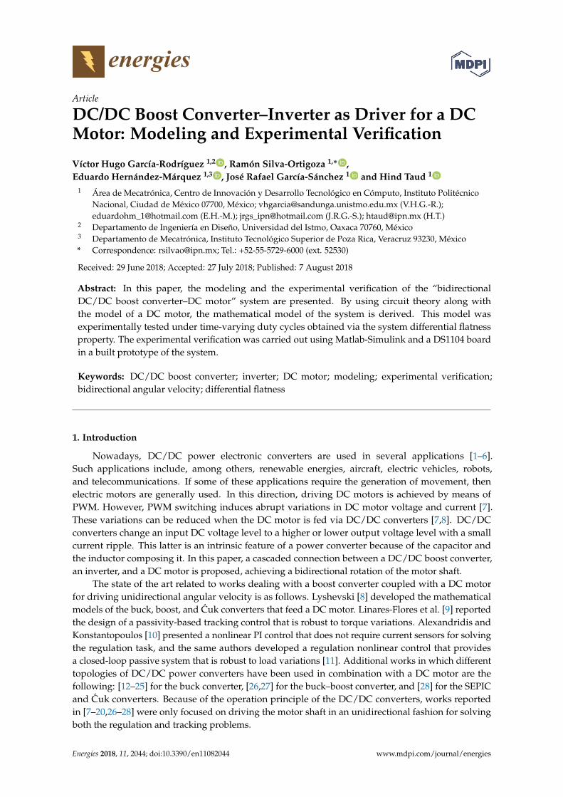
Figure 1 shows the electronic circuit of the DC/DC boost converter–inverter–DC motor system.This system is composed by the following:

• DC/DC boost converter. This is composed of a power supply E, a switching input u1 that turnson/off transistor Q1, a current i that flows through the inductor L, and a diode D. The outputvoltage, associated with capacitor C and load R, is denoted by υ.

• Inverter. Here, u2 and u2 are the inputs that turn on/off transistors Q2 and Q2, respectively, thusachieving the bidirectional rotation of the motor shaft.

• DC motor. Parameters ia, Ra, and La are the armature current, armature resistance, and armatureinductance; ω denotes the angular velocity of the motor shaft. Additional parameters for theDC motor are J, ke, km, and b, which correspond to the moment of inertia of the rotor and load,the counter-electromotive force constant, the torque constant, and the viscous friction coefficient,respectively.

Figure 1. DC/DC boost converter–inverter–DC motor system.

Energies 2018, 11, 2044 3 of 15

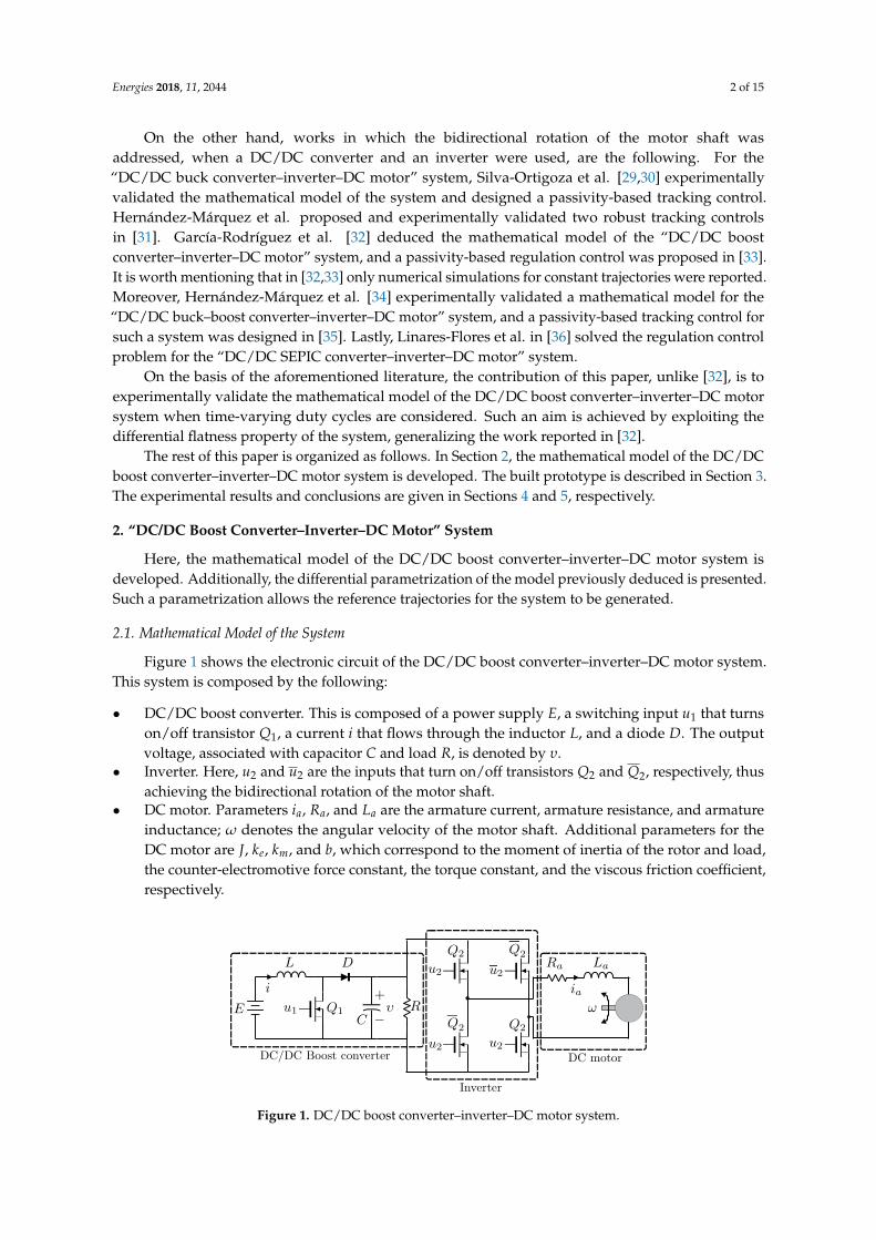
The ideal circuit depicted in Figure 2, which is associated with Figure 1, was used to develop themathematical model of the system. The model was obtained by applying Kirchhoff’s current law andKirchhoff’s voltage law to node A and mesh I (see Figure 2) and, also, by considering the mathematicalmodel of a DC motor [37].

Figure 2. Ideal circuit of DC/DC boost converter–inverter–DC motor system.

The operation modes of the electronic circuit shown in Figure 2 are described below.These operation modes appear when transistors are on (i.e., u1 = 1 or u2 = 1) or off (i.e., u1 = 0 oru2 = −1) generating the following four operation modes.

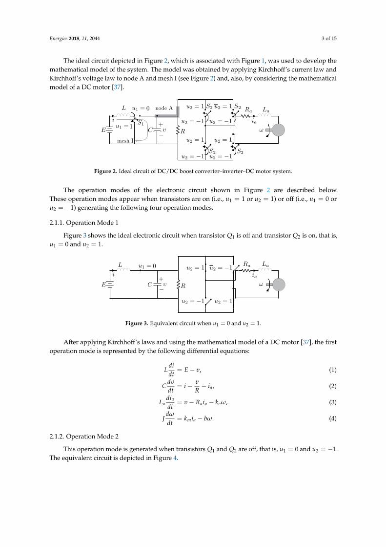
2.1.1. Operation Mode 1

Figure 3 shows the ideal electronic circuit when transistor Q1 is off and transistor Q2 is on, that is,u1 = 0 and u2 = 1.

Figure 3. Equivalent circuit when u1 = 0 and u2 = 1.

After applying Kirchhoff’s laws and using the mathematical model of a DC motor [37], the firstoperation mode is represented by the following differential equations:

Ldidt

= E− υ, (1)

Cdυ

dt= i− υ

R− ia, (2)

Ladia

dt= υ− Raia − keω, (3)

Jdω

dt= kmia − bω. (4)

2.1.2. Operation Mode 2

This operation mode is generated when transistors Q1 and Q2 are off, that is, u1 = 0 and u2 = −1.The equivalent circuit is depicted in Figure 4.

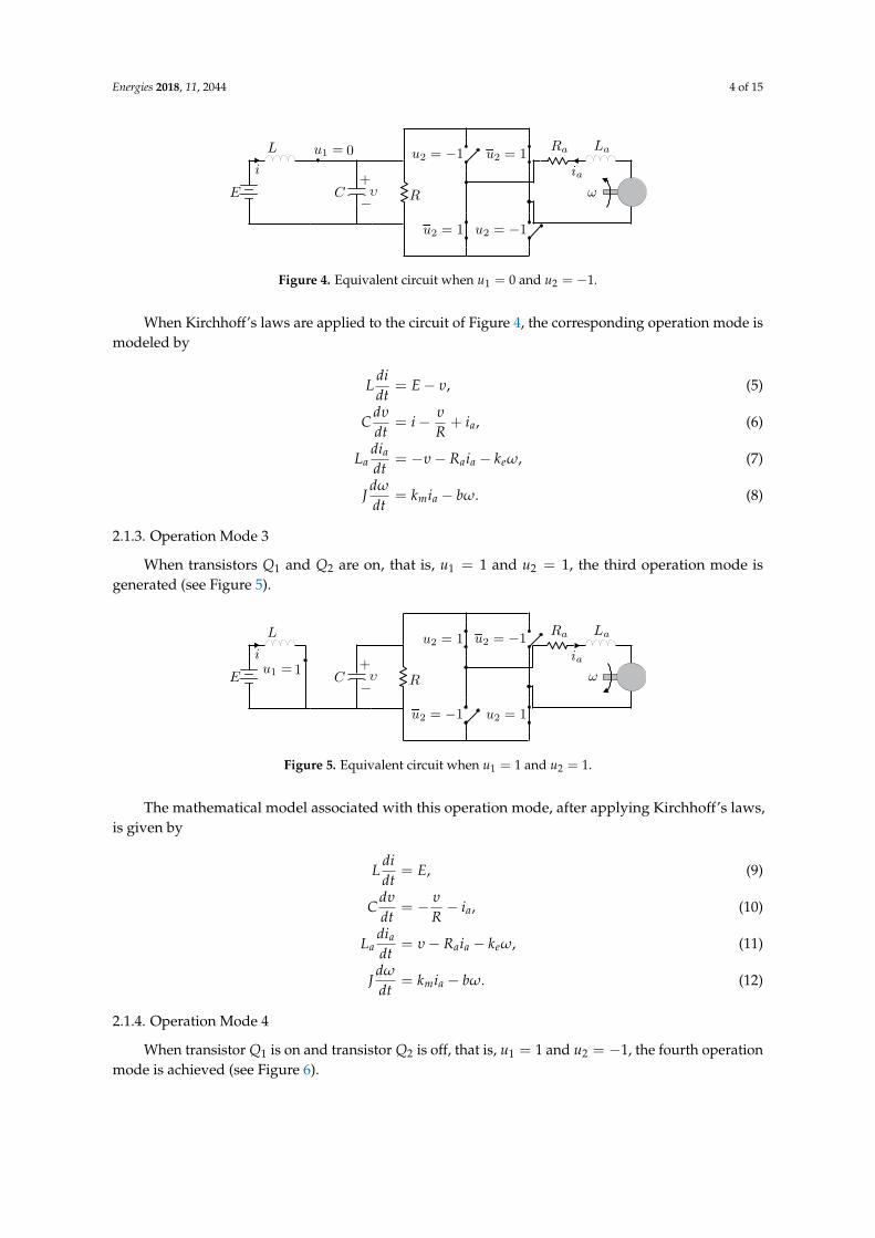
Energies 2018, 11, 2044 4 of 15

Figure 4. Equivalent circuit when u1 = 0 and u2 = −1.

When Kirchhoff’s laws are applied to the circuit of Figure 4, the corresponding operation mode ismodeled by

Ldidt

= E− υ, (5)

Cdυ

dt= i− υ

R+ ia, (6)

Ladia

dt= −υ− Raia − keω, (7)

Jdω

dt= kmia − bω. (8)

2.1.3. Operation Mode 3

When transistors Q1 and Q2 are on, that is, u1 = 1 and u2 = 1, the third operation mode isgenerated (see Figure 5).

Figure 5. Equivalent circuit when u1 = 1 and u2 = 1.

The mathematical model associated with this operation mode, after applying Kirchhoff’s laws,is given by

Ldidt

= E, (9)

Cdυ

dt= − υ

R− ia, (10)

Ladia

dt= υ− Raia − keω, (11)

Jdω

dt= kmia − bω. (12)

2.1.4. Operation Mode 4

When transistor Q1 is on and transistor Q2 is off, that is, u1 = 1 and u2 = −1, the fourth operationmode is achieved (see Figure 6).

Energies 2018, 11, 2044 5 of 15

Figure 6. Equivalent circuit when u1 = 1 and u2 = −1.

In this case, the operation mode is modeled by the following differential equations:

Ldidt

= E, (13)

Cdυ

dt= − υ

R+ ia, (14)

Ladia

dt= −υ− Raia − keω, (15)

Jdω

dt= kmia − bω. (16)

After combining the four operation modes, given by Equations (1)–(16), the mathematical modelof the DC/DC boost converter–inverter–DC motor system is determined by

Ldidt

= −(1− u1)υ + E, (17)

Cdυ

dt= (1− u1)i−

υ

R− iau2, (18)

Ladia

dt= υu2 − Raia − keω, (19)

Jdω

dt= kmia − bω, (20)

where u1 and u2 represent the switches’ positions. The mathematical model given byEquations (17)–(20) is known as the switched model because of its binary-valued nature. The averagemodel associated with Equations (17)–(20) is as follows:

Ldidt

= −(1− u1av)υ + E, (21)

Cdυ

dt= (1− u1av)i−

υ

R− iau2av, (22)

Ladia

dt= υu2av − Raia − keω, (23)

Jdω

dt= kmia − bω, (24)

where u1av ∈ [0, 1) and u2av ∈ [−1, 1].

2.2. Generation of Reference Trajectories

The differential parameterization of the average system given by Equations (21)–(24) ispresented below.

The flat output of the boost converter, according to [38,39], is determined by its energy; that is,

E =12(Li2 + Cυ2). (25)

Energies 2018, 11, 2044 6 of 15

The flat output of a DC motor, according to [15], is given by the angular velocity of the motor shaftω. After proposing the flat outputs of the DC/DC boost converter–inverter–DC motor average systemas F1 = E and F2 = ω, the following differential parameterization associated to Equations (21)–(24)is found:

i = −RCE2L

+ α, (26)

υ =

[R(−RCE2

2L+ αE− βia − F1

)]1/2

, (27)

ia =1

km

(JF2 + bF2

), (28)

ω = F2, (29)

u1av =1γ

[F1 −

E2

L− 2

R2Cυ2 − 3

RCiaυu2av −

1C

i2au22av

]+ 1, (30)

u2av =β

υ, (31)

with

α =

(RCE2L

)2+

1L[CR(

βia + F1)+ 2F1

]1/2

,

β = Ladia

dt+ Raia + keF2,

γ =EL

υ +2

RCiυ +

1C

iiau2av.

As can be observed, the average model given by Equations (21)–(24) is now represented by thedifferential parameterization given by Equations (26)–(31) expressed in terms of variables F1 andF2 and their corresponding derivatives with respect to time. Such a representation, compared toEquations (21)–(24), allows the reference trajectories associated with states i, υ, and ia and inputs u1avand u2av to be found offline [38]. Thus, when F1 and F2 are replaced by E∗ and ω∗ in Equations (26)–(31),the reference trajectories are obtained; this is, i∗, υ∗, i∗a , u∗1av, and u∗2av. Here, E∗ is the desired boostconverter energy and ω∗ represents the desired angular velocity of the motor shaft.

3. Built Experimental Prototype

In this section, the experimental platform used to validate the mathematical model of the boostconverter–inverter–DC motor system is described.

A schematic diagram of the built platform is presented in Figure 7 and is composed ofthe following blocks:

• DC/DC boost converter–inverter–DC motor system. The following three subsystems are distinguishedwithin this block: boost converter, inverter, and DC motor. In this direction, the nominal valuesassociated with the converter parameters are

L = 4.94 mH, R = 64 Ω, C = 114.4 µF, E = 12 V.

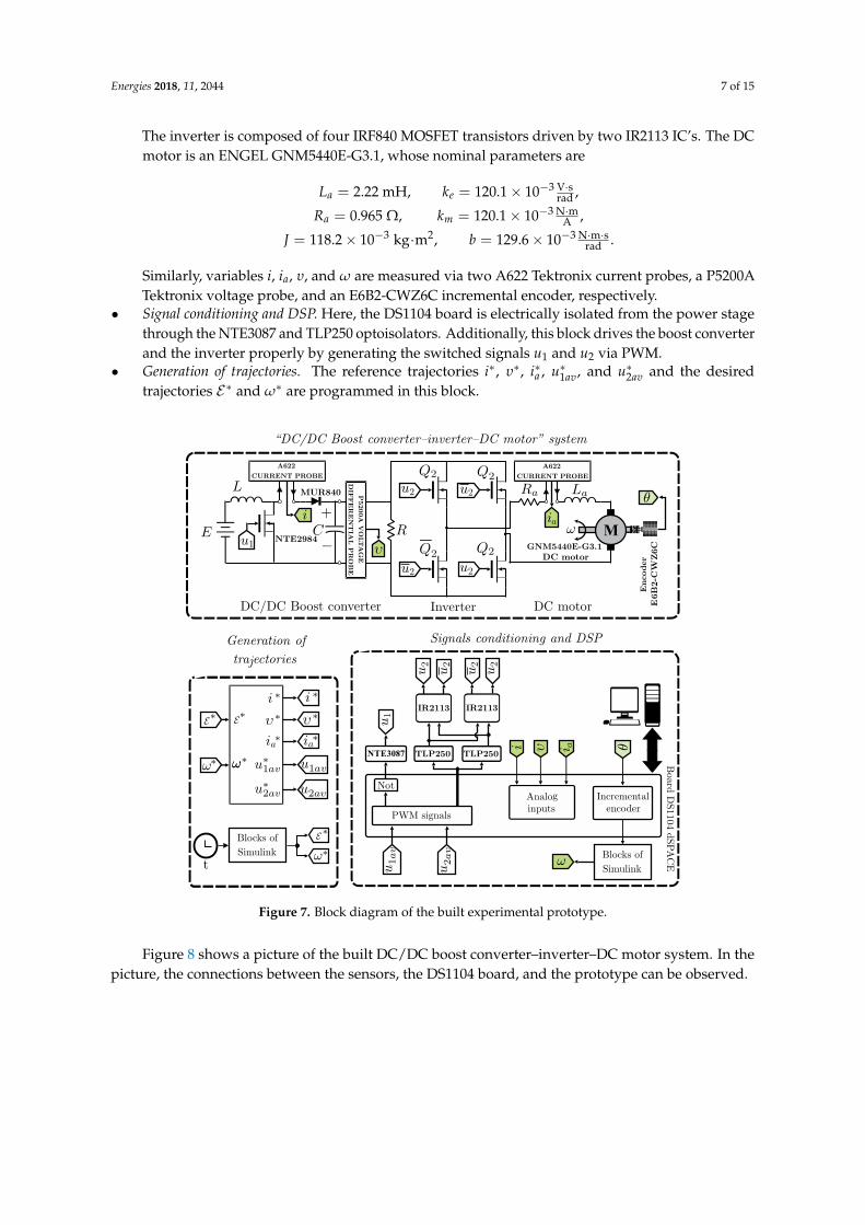
Energies 2018, 11, 2044 7 of 15

The inverter is composed of four IRF840 MOSFET transistors driven by two IR2113 IC’s. The DCmotor is an ENGEL GNM5440E-G3.1, whose nominal parameters are

La = 2.22 mH, ke = 120.1× 10−3 V·srad ,

Ra = 0.965 Ω, km = 120.1× 10−3 N·mA ,

J = 118.2× 10−3 kg·m2, b = 129.6× 10−3 N·m·srad .

Similarly, variables i, ia, υ, and ω are measured via two A622 Tektronix current probes, a P5200ATektronix voltage probe, and an E6B2-CWZ6C incremental encoder, respectively.

• Signal conditioning and DSP. Here, the DS1104 board is electrically isolated from the power stagethrough the NTE3087 and TLP250 optoisolators. Additionally, this block drives the boost converterand the inverter properly by generating the switched signals u1 and u2 via PWM.

• Generation of trajectories. The reference trajectories i∗, υ∗, i∗a , u∗1av, and u∗2av and the desiredtrajectories E∗ and ω∗ are programmed in this block.

Figure 7. Block diagram of the built experimental prototype.

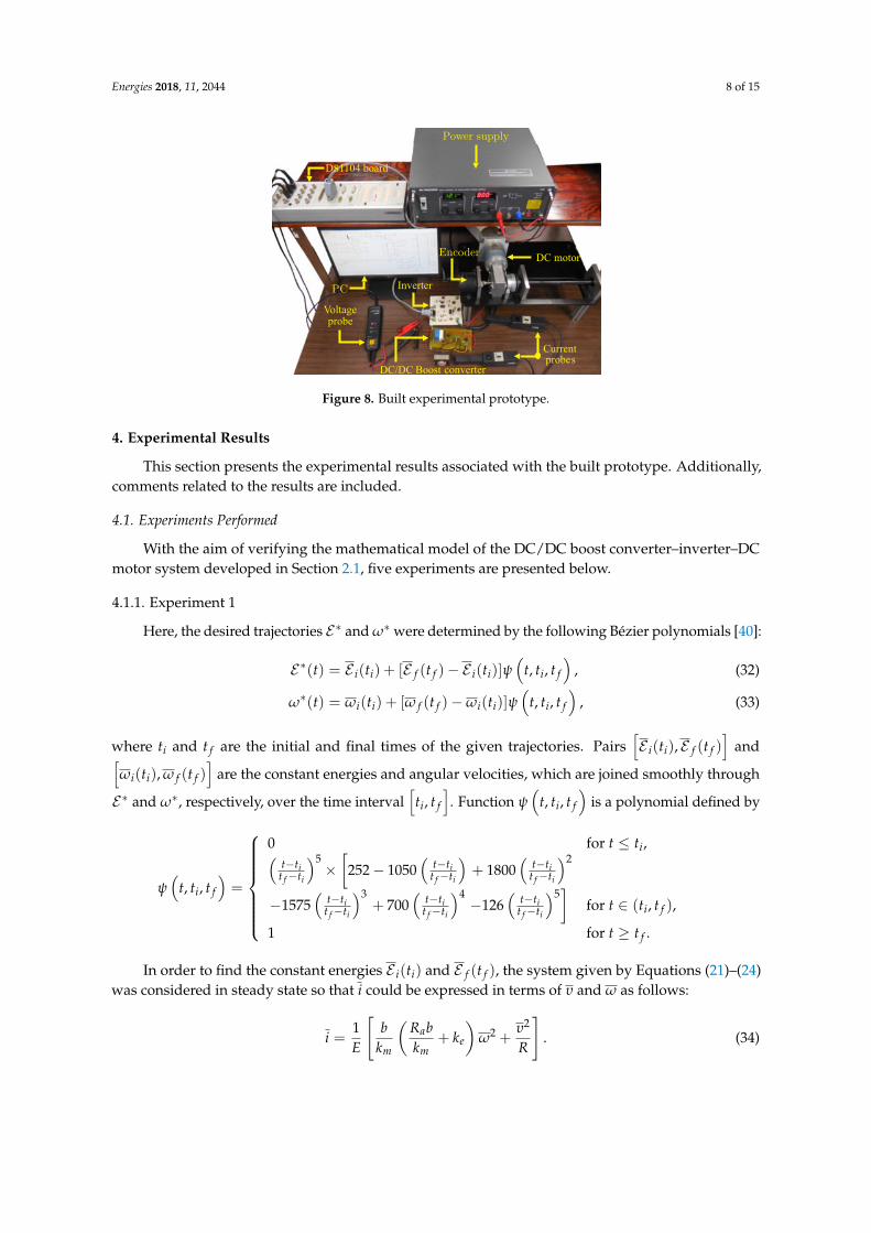
Figure 8 shows a picture of the built DC/DC boost converter–inverter–DC motor system. In thepicture, the connections between the sensors, the DS1104 board, and the prototype can be observed.

Energies 2018, 11, 2044 8 of 15

Figure 8. Built experimental prototype.

4. Experimental Results

This section presents the experimental results associated with the built prototype. Additionally,comments related to the results are included.

4.1. Experiments Performed

With the aim of verifying the mathematical model of the DC/DC boost converter–inverter–DCmotor system developed in Section 2.1, five experiments are presented below.

4.1.1. Experiment 1

Here, the desired trajectories E∗ and ω∗ were determined by the following Bézier polynomials [40]:

E∗(t) = E i(ti) + [E f (t f )− E i(ti)]ψ(

t, ti, t f

), (32)

ω∗(t) = ωi(ti) + [ω f (t f )−ωi(ti)]ψ(

t, ti, t f

), (33)

where ti and t f are the initial and final times of the given trajectories. Pairs[E i(ti), E f (t f )

]and[

ωi(ti), ω f (t f )]

are the constant energies and angular velocities, which are joined smoothly through

E∗ and ω∗, respectively, over the time interval[ti, t f

]. Function ψ

(t, ti, t f

)is a polynomial defined by

ψ(

t, ti, t f

)=

0 for t ≤ ti,(t−ti

t f−ti

)5×[

252− 1050(

t−tit f−ti

)+ 1800

(t−ti

t f−ti

)2

−1575(

t−tit f−ti

)3+ 700

(t−ti

t f−ti

)4−126

(t−ti

t f−ti

)5]

for t ∈ (ti, t f ),

1 for t ≥ t f .

In order to find the constant energies E i(ti) and E f (t f ), the system given by Equations (21)–(24)was considered in steady state so that i could be expressed in terms of υ and ω as follows:

i =1E

[b

km

(Rabkm

+ ke

)ω2 +

υ2

R

]. (34)

Energies 2018, 11, 2044 9 of 15

When Equation (34) was replaced in Equation (25), the constant energies E i(ti) and E f (t f ) wereobtained and were given by

E i(ti) =12

LE2

[b

km

(Rabkm

+ ke

)ω2

i +υ2

iR

]2

+12

C υ2i , (35)

E f (t f ) =12

LE2

[b

km

(Rabkm

+ ke

)ω2

f +υ2

f

R

]2

+12

C υ2f . (36)

In this experiment, the constant voltages and angular velocities,[υi, υ f

]and

[ωi, ω f

], associated

to E∗ and ω∗, were chosen as

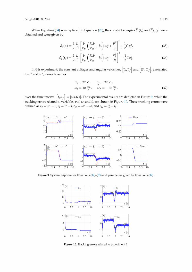
υi = 27 V, υ f = 32 V,

ωi = 10 rads , ω f = −10 rad

s , (37)

over the time interval[ti, t f

]= [4 s, 6 s]. The experimental results are depicted in Figure 9, while the

tracking errors related to variables υ, i, ω, and ia are shown in Figure 10. These tracking errors weredefined as eυ = υ∗ − υ, ei = i∗ − i, eω = ω∗ −ω, and eia = i∗a − ia.

0 2.5 5 7.5 100

10

20

30

40

t [s]

[V]

υ υ∗

0 2.5 5 7.5 10

0

1

2

3

t [s]

[A]

i i∗

0 2.5 5 7.5 100

0.25

0.5

0.75

1

t [s]

u1av

0 2.5 5 7.5 10−20

−10

0

10

20

t [s]

[rad s]

ω ω∗

0 2.5 5 7.5 10−2

−1

0

1

2

t [s]

[A]

ia i∗

a

0 2.5 5 7.5 10−1

−0.5

0

0.5

1

t [s]

u2av

Figure 9. System response for Equations (32)–(33) and parameters given by Equations (37).

0 2.5 5 7.5 10

0

10

20

30

0 2.5 5 7.5 10

-1

0

1

2

0 2.5 5 7.5 10

0

5

10

0 2.5 5 7.5 10

-1

0

1

Figure 10. Tracking errors related to experiment 1.

Energies 2018, 11, 2044 10 of 15

4.1.2. Experiment 2

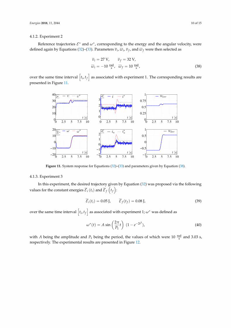
Reference trajectories E∗ and ω∗, corresponding to the energy and the angular velocity, weredefined again by Equations (32)–(33). Parameters υi, ωi, υ f , and ω f were then selected as

υi = 27 V, υ f = 32 V,

ωi = −10 rads , ω f = 10 rad

s , (38)

over the same time interval[ti, t f

]as associated with experiment 1. The corresponding results are

presented in Figure 11.

0 2.5 5 7.5 100

10

20

30

40

t [s]

[V]

υ υ∗

0 2.5 5 7.5 10

0

1

2

3

t [s]

[A]

i i∗

0 2.5 5 7.5 100

0.25

0.5

0.75

1

t [s]

u1av

0 2.5 5 7.5 10−20

−10

0

10

20

t [s]

[rad s]

ω ω∗

0 2.5 5 7.5 10−2

−1

0

1

2

t [s]

[A]

ia i∗

a

0 2.5 5 7.5 10−1

−0.5

0

0.5

1

t [s]

u2av

Figure 11. System response for Equations (32)–(33) and parameters given by Equation (38).

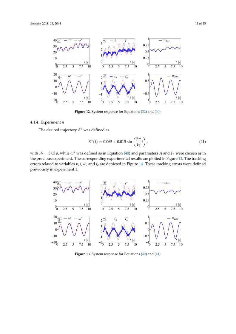
4.1.3. Experiment 3

In this experiment, the desired trajectory given by Equation (32) was proposed via the followingvalues for the constant energies E i (ti) and E f

(t f

):

E i(ti) = 0.05 J, E f (t f ) = 0.08 J, (39)

over the same time interval[ti, t f

]as associated with experiment 1; ω∗ was defined as

ω∗(t) = A sin(

2π

P1t)

(1− e−2t3), (40)

with A being the amplitude and P1 being the period, the values of which were 10 rads and 3.03 s,

respectively. The experimental results are presented in Figure 12.

Energies 2018, 11, 2044 11 of 15

0 2.5 5 7.5 100

10

20

30

40

t [s]

[V]

υ υ∗

0 2.5 5 7.5 10

0

1

2

3

t [s]

[A]

i i∗

0 2.5 5 7.5 100

0.25

0.5

0.75

1

t [s]

u1av

0 2.5 5 7.5 10−20

−10

0

10

20

t [s]

[rad s]

ω ω∗

0 2.5 5 7.5 10−2

−1

0

1

2

t [s]

[A]

ia i∗

a

0 2.5 5 7.5 10−1

−0.5

0

0.5

1

t [s]

u2av

Figure 12. System response for Equations (32) and (40).

4.1.4. Experiment 4

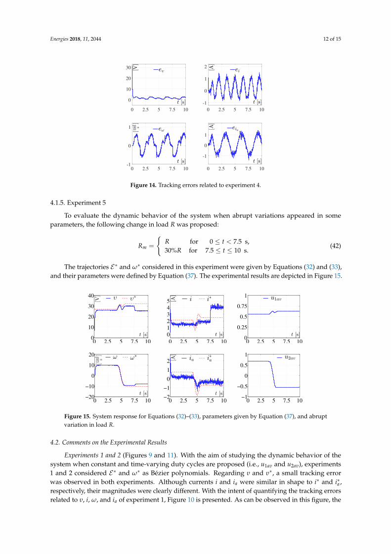
The desired trajectory E∗ was defined as

E∗(t) = 0.065 + 0.015 sin(

2π

P2t)

, (41)

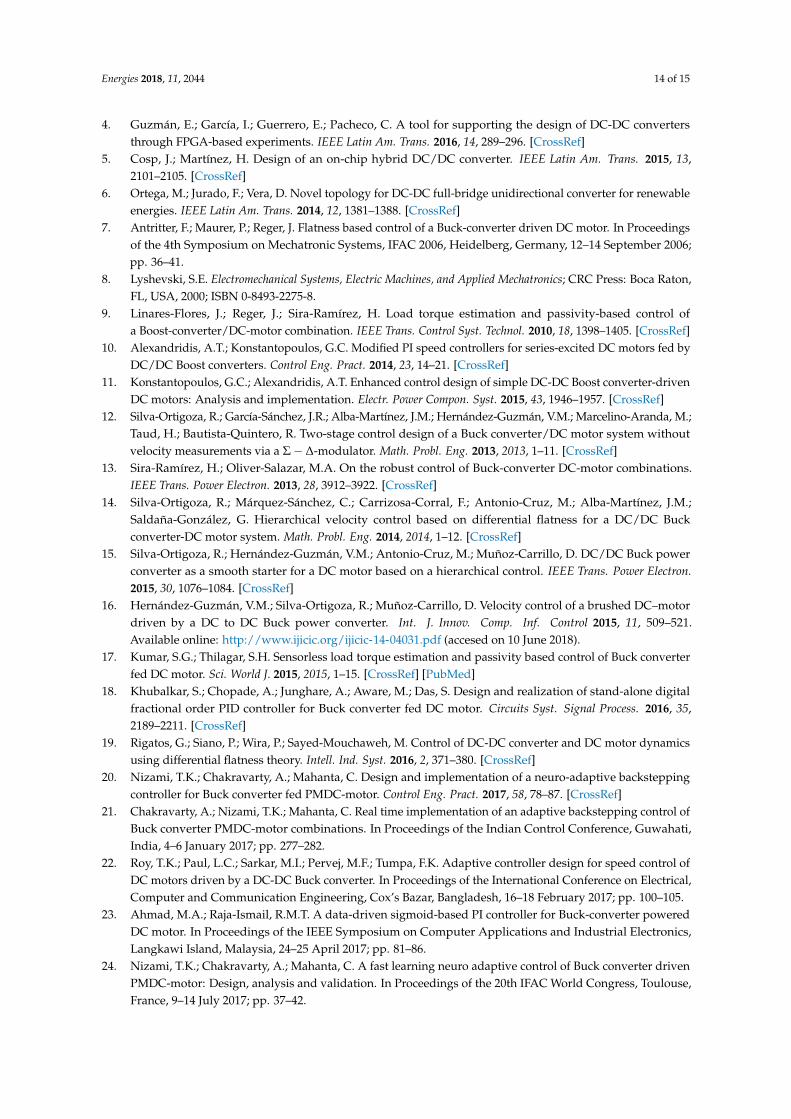
with P2 = 3.03 s, while ω∗ was defined as in Equation (40) and parameters A and P1 were chosen as inthe previous experiment. The corresponding experimental results are plotted in Figure 13. The trackingerrors related to variables υ, i, ω, and ia are depicted in Figure 14. These tracking errors were definedpreviously in experiment 1.

0 2.5 5 7.5 100

10

20

30

40

t [s]

[V]

υ υ∗

0 2.5 5 7.5 10

0

1

2

3

t [s]

[A]

i i∗

0 2.5 5 7.5 100

0.25

0.5

0.75

1

t [s]

u1av

0 2.5 5 7.5 10−20

−10

0

10

20

t [s]

[rad s]

ω ω∗

0 2.5 5 7.5 10−2

−1

0

1

2

t [s]

[A]

ia i∗

a

0 2.5 5 7.5 10−1

−0.5

0

0.5

1

t [s]

u2av

Figure 13. System response for Equations (40) and (41).

Energies 2018, 11, 2044 12 of 15

0 2.5 5 7.5 10

0

10

20

30

0 2.5 5 7.5 10

-1

0

1

2

0 2.5 5 7.5 10-1

0

1

0 2.5 5 7.5 10

-1

0

1

Figure 14. Tracking errors related to experiment 4.

4.1.5. Experiment 5

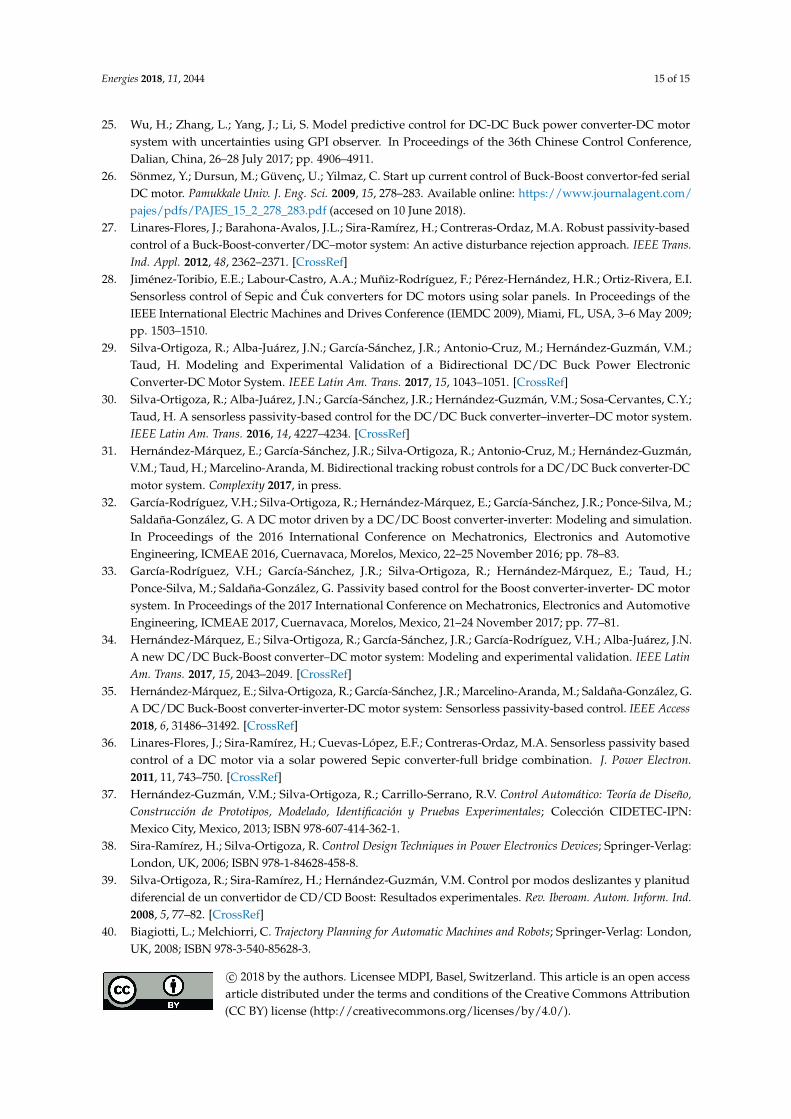
To evaluate the dynamic behavior of the system when abrupt variations appeared in someparameters, the following change in load R was proposed:

Rm =

R for 0 ≤ t < 7.5 s,30%R for 7.5 ≤ t ≤ 10 s.

(42)

The trajectories E∗ and ω∗ considered in this experiment were given by Equations (32) and (33),and their parameters were defined by Equation (37). The experimental results are depicted in Figure 15.

0 2.5 5 7.5 100

10

20

30

40

t [s]

[V]

υ υ∗

0 2.5 5 7.5 10

0

1

2

3

4

5

t [s]

[A]

i i∗

0 2.5 5 7.5 100

0.25

0.5

0.75

1

t [s]

u1av

0 2.5 5 7.5 10−20

−10

0

10

20

t [s]

[rad s]

ω ω∗

0 2.5 5 7.5 10−2

−1

0

1

2

t [s]

[A]

ia i∗

a

0 2.5 5 7.5 10−1

−0.5

0

0.5

1

u2av

Figure 15. System response for Equations (32)–(33), parameters given by Equation (37), and abruptvariation in load R.

4.2. Comments on the Experimental Results

Experiments 1 and 2 (Figures 9 and 11). With the aim of studying the dynamic behavior of thesystem when constant and time-varying duty cycles are proposed (i.e., u1av and u2av), experiments1 and 2 considered E∗ and ω∗ as Bézier polynomials. Regarding υ and υ∗, a small tracking errorwas observed in both experiments. Although currents i and ia were similar in shape to i∗ and i∗a ,respectively, their magnitudes were clearly different. With the intent of quantifying the tracking errorsrelated to υ, i, ω, and ia of experiment 1, Figure 10 is presented. As can be observed in this figure, the

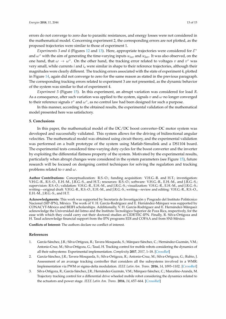
Energies 2018, 11, 2044 13 of 15

errors do not converge to zero due to parasitic resistances, and energy losses were not considered inthe mathematical model. Concerning experiment 2, the corresponding errors are not plotted, as theproposed trajectories were similar to those of experiment 1.

Experiments 3 and 4 (Figures 12 and 13). Here, appropriate trajectories were considered for E∗and ω∗ with the aim of generating the time-varying inputs u1av and u2av. It was also observed, on theone hand, that ω → ω∗. On the other hand, the tracking error related to voltages υ and υ∗ wasvery small, while currents i and ia were similar in shape to their reference trajectories, although theirmagnitudes were clearly different. The tracking errors associated with the state of experiment 4, plottedin Figure 14, again did not converge to zero for the same reason as stated in the previous paragraph.The corresponding tracking errors related to experiment 3 are not presented, as the dynamic behaviorof the system was similar to that of experiment 4.

Experiment 5 (Figure 15). In this experiment, an abrupt variation was considered for load R.As a consequence, after such variation was applied to the system, signals υ and ω no longer convergedto their reference signals υ∗ and ω∗, as no control law had been designed for such a purpose.

In this manner, according to the obtained results, the experimental validation of the mathematicalmodel presented here was satisfactory.

5. Conclusions

In this paper, the mathematical model of the DC/DC boost converter–DC motor system wasdeveloped and successfully validated. This system allows for the driving of bidirectional angularvelocities. The mathematical model was obtained using circuit theory, and the experimental validationwas performed on a built prototype of the system using Matlab-Simulink and a DS1104 board.The experimental tests considered time-varying duty cycles for the boost converter and the inverterby exploiting the differential flatness property of the system. Motivated by the experimental results,particularly when abrupt changes were considered in the system parameters (see Figure 15), futureresearch will be focused on designing control techniques for solving the regulation and trackingproblems related to υ and ω.

Author Contributions: Conceptualization: R.S.-O.; funding acquisition: V.H.G.-R. and H.T.; investigation:V.H.G.-R., R.S.-O., E.H.-M., J.R.G.-S., and H.T.; resources: R.S.-O.; software: V.H.G.-R., E.H.-M., and J.R.G.-S.;supervision: R.S.-O.; validation: V.H.G.-R., E.H.-M., and J.R.G.-S.; visualization: V.H.G.-R., E.H.-M., and J.R.G.-S.;writing—original draft: V.H.G.-R., R.S.-O., E.H.-M., and J.R.G.-S.; writing—review and editing: V.H.G.-R., R.S.-O.,E.H.-M., J.R.G.-S., and H.T.

Acknowledgments: This work was supported by Secretaría de Investigación y Posgrado del Instituto PolitécnicoNacional (SIP-IPN), México. The work of V. H. García-Rodríguez and E. Hernández-Márquez was supported byCONACYT-México and BEIFI scholarships. Additionally, V. H. García-Rodríguez and E. Hernández-Márquezacknowledge the Universidad del Istmo and the Instituto Tecnológico Superior de Poza Rica, respectively, for theease with which they could carry out their doctoral studies at CIDETEC-IPN. Finally, R. Silva-Ortigoza andH. Taud acknowledge financial support from the IPN programs EDI and COFAA and from SNI-México.

Conflicts of Interest: The authors declare no conflict of interest.

References

1. García-Sánchez, J.R.; Silva-Ortigoza, R.; Tavera-Mosqueda, S.; Márquez-Sánchez, C.; Hernández-Guzmán, V.M.;Antonio-Cruz, M.; Silva-Ortigoza, G.; Taud, H. Tracking control for mobile robots considering the dynamics ofall their subsystems: Experimental implementation. Complexity 2017, 2017, 1–18. [CrossRef]

2. García-Sánchez, J.R.; Tavera-Mosqueda, S.; Silva-Ortigoza, R.; Antonio-Cruz, M.; Silva-Ortigoza, G.; Rubio, J.Assessment of an avarage tracking controller that considers all the subsystems involved in a WMR:Implementation via PWM or sigma-delta modulation. IEEE Latin Am. Trans. 2016, 14, 1093–1102. [CrossRef]

3. Silva-Ortigoza, R.; García-Sánchez, J.R.; Hernández-Guzmán, V.M.; Márquez-Sánchez, C.; Marcelino-Aranda, M.Trajectory tracking control for a differential drive wheeled mobile robot considering the dynamics related tothe actuators and power stage. IEEE Latin Am. Trans. 2016, 14, 657–664. [CrossRef]

Energies 2018, 11, 2044 14 of 15

4. Guzmán, E.; García, I.; Guerrero, E.; Pacheco, C. A tool for supporting the design of DC-DC convertersthrough FPGA-based experiments. IEEE Latin Am. Trans. 2016, 14, 289–296. [CrossRef]

5. Cosp, J.; Martínez, H. Design of an on-chip hybrid DC/DC converter. IEEE Latin Am. Trans. 2015, 13,2101–2105. [CrossRef]

6. Ortega, M.; Jurado, F.; Vera, D. Novel topology for DC-DC full-bridge unidirectional converter for renewableenergies. IEEE Latin Am. Trans. 2014, 12, 1381–1388. [CrossRef]

7. Antritter, F.; Maurer, P.; Reger, J. Flatness based control of a Buck-converter driven DC motor. In Proceedingsof the 4th Symposium on Mechatronic Systems, IFAC 2006, Heidelberg, Germany, 12–14 September 2006;pp. 36–41.

8. Lyshevski, S.E. Electromechanical Systems, Electric Machines, and Applied Mechatronics; CRC Press: Boca Raton,FL, USA, 2000; ISBN 0-8493-2275-8.

9. Linares-Flores, J.; Reger, J.; Sira-Ramírez, H. Load torque estimation and passivity-based control ofa Boost-converter/DC-motor combination. IEEE Trans. Control Syst. Technol. 2010, 18, 1398–1405. [CrossRef]

10. Alexandridis, A.T.; Konstantopoulos, G.C. Modified PI speed controllers for series-excited DC motors fed byDC/DC Boost converters. Control Eng. Pract. 2014, 23, 14–21. [CrossRef]

11. Konstantopoulos, G.C.; Alexandridis, A.T. Enhanced control design of simple DC-DC Boost converter-drivenDC motors: Analysis and implementation. Electr. Power Compon. Syst. 2015, 43, 1946–1957. [CrossRef]

12. Silva-Ortigoza, R.; García-Sánchez, J.R.; Alba-Martínez, J.M.; Hernández-Guzmán, V.M.; Marcelino-Aranda, M.;Taud, H.; Bautista-Quintero, R. Two-stage control design of a Buck converter/DC motor system withoutvelocity measurements via a Σ− ∆-modulator. Math. Probl. Eng. 2013, 2013, 1–11. [CrossRef]

13. Sira-Ramírez, H.; Oliver-Salazar, M.A. On the robust control of Buck-converter DC-motor combinations.IEEE Trans. Power Electron. 2013, 28, 3912–3922. [CrossRef]

14. Silva-Ortigoza, R.; Márquez-Sánchez, C.; Carrizosa-Corral, F.; Antonio-Cruz, M.; Alba-Martínez, J.M.;Saldaña-González, G. Hierarchical velocity control based on differential flatness for a DC/DC Buckconverter-DC motor system. Math. Probl. Eng. 2014, 2014, 1–12. [CrossRef]

15. Silva-Ortigoza, R.; Hernández-Guzmán, V.M.; Antonio-Cruz, M.; Muñoz-Carrillo, D. DC/DC Buck powerconverter as a smooth starter for a DC motor based on a hierarchical control. IEEE Trans. Power Electron.2015, 30, 1076–1084. [CrossRef]

16. Hernández-Guzmán, V.M.; Silva-Ortigoza, R.; Muñoz-Carrillo, D. Velocity control of a brushed DC–motordriven by a DC to DC Buck power converter. Int. J. Innov. Comp. Inf. Control 2015, 11, 509–521.Available online: http://www.ijicic.org/ijicic-14-04031.pdf (accesed on 10 June 2018).

17. Kumar, S.G.; Thilagar, S.H. Sensorless load torque estimation and passivity based control of Buck converterfed DC motor. Sci. World J. 2015, 2015, 1–15. [CrossRef] [PubMed]

18. Khubalkar, S.; Chopade, A.; Junghare, A.; Aware, M.; Das, S. Design and realization of stand-alone digitalfractional order PID controller for Buck converter fed DC motor. Circuits Syst. Signal Process. 2016, 35,2189–2211. [CrossRef]

19. Rigatos, G.; Siano, P.; Wira, P.; Sayed-Mouchaweh, M. Control of DC-DC converter and DC motor dynamicsusing differential flatness theory. Intell. Ind. Syst. 2016, 2, 371–380. [CrossRef]

20. Nizami, T.K.; Chakravarty, A.; Mahanta, C. Design and implementation of a neuro-adaptive backsteppingcontroller for Buck converter fed PMDC-motor. Control Eng. Pract. 2017, 58, 78–87. [CrossRef]

21. Chakravarty, A.; Nizami, T.K.; Mahanta, C. Real time implementation of an adaptive backstepping control ofBuck converter PMDC-motor combinations. In Proceedings of the Indian Control Conference, Guwahati,India, 4–6 January 2017; pp. 277–282.

22. Roy, T.K.; Paul, L.C.; Sarkar, M.I.; Pervej, M.F.; Tumpa, F.K. Adaptive controller design for speed control ofDC motors driven by a DC-DC Buck converter. In Proceedings of the International Conference on Electrical,Computer and Communication Engineering, Cox’s Bazar, Bangladesh, 16–18 February 2017; pp. 100–105.

23. Ahmad, M.A.; Raja-Ismail, R.M.T. A data-driven sigmoid-based PI controller for Buck-converter poweredDC motor. In Proceedings of the IEEE Symposium on Computer Applications and Industrial Electronics,Langkawi Island, Malaysia, 24–25 April 2017; pp. 81–86.

24. Nizami, T.K.; Chakravarty, A.; Mahanta, C. A fast learning neuro adaptive control of Buck converter drivenPMDC-motor: Design, analysis and validation. In Proceedings of the 20th IFAC World Congress, Toulouse,France, 9–14 July 2017; pp. 37–42.

Energies 2018, 11, 2044 15 of 15

25. Wu, H.; Zhang, L.; Yang, J.; Li, S. Model predictive control for DC-DC Buck power converter-DC motorsystem with uncertainties using GPI observer. In Proceedings of the 36th Chinese Control Conference,Dalian, China, 26–28 July 2017; pp. 4906–4911.

26. Sönmez, Y.; Dursun, M.; Güvenç, U.; Yilmaz, C. Start up current control of Buck-Boost convertor-fed serialDC motor. Pamukkale Univ. J. Eng. Sci. 2009, 15, 278–283. Available online: https://www.journalagent.com/pajes/pdfs/PAJES_15_2_278_283.pdf (accesed on 10 June 2018).

27. Linares-Flores, J.; Barahona-Avalos, J.L.; Sira-Ramírez, H.; Contreras-Ordaz, M.A. Robust passivity-basedcontrol of a Buck-Boost-converter/DC–motor system: An active disturbance rejection approach. IEEE Trans.Ind. Appl. 2012, 48, 2362–2371. [CrossRef]

28. Jiménez-Toribio, E.E.; Labour-Castro, A.A.; Muñiz-Rodríguez, F.; Pérez-Hernández, H.R.; Ortiz-Rivera, E.I.Sensorless control of Sepic and Cuk converters for DC motors using solar panels. In Proceedings of theIEEE International Electric Machines and Drives Conference (IEMDC 2009), Miami, FL, USA, 3–6 May 2009;pp. 1503–1510.

29. Silva-Ortigoza, R.; Alba-Juárez, J.N.; García-Sánchez, J.R.; Antonio-Cruz, M.; Hernández-Guzmán, V.M.;Taud, H. Modeling and Experimental Validation of a Bidirectional DC/DC Buck Power ElectronicConverter-DC Motor System. IEEE Latin Am. Trans. 2017, 15, 1043–1051. [CrossRef]

30. Silva-Ortigoza, R.; Alba-Juárez, J.N.; García-Sánchez, J.R.; Hernández-Guzmán, V.M.; Sosa-Cervantes, C.Y.;Taud, H. A sensorless passivity-based control for the DC/DC Buck converter–inverter–DC motor system.IEEE Latin Am. Trans. 2016, 14, 4227–4234. [CrossRef]

31. Hernández-Márquez, E.; García-Sánchez, J.R.; Silva-Ortigoza, R.; Antonio-Cruz, M.; Hernández-Guzmán,V.M.; Taud, H.; Marcelino-Aranda, M. Bidirectional tracking robust controls for a DC/DC Buck converter-DCmotor system. Complexity 2017, in press.

32. García-Rodríguez, V.H.; Silva-Ortigoza, R.; Hernández-Márquez, E.; García-Sánchez, J.R.; Ponce-Silva, M.;Saldaña-González, G. A DC motor driven by a DC/DC Boost converter-inverter: Modeling and simulation.In Proceedings of the 2016 International Conference on Mechatronics, Electronics and AutomotiveEngineering, ICMEAE 2016, Cuernavaca, Morelos, Mexico, 22–25 November 2016; pp. 78–83.

33. García-Rodríguez, V.H.; García-Sánchez, J.R.; Silva-Ortigoza, R.; Hernández-Márquez, E.; Taud, H.;Ponce-Silva, M.; Saldaña-González, G. Passivity based control for the Boost converter-inverter- DC motorsystem. In Proceedings of the 2017 International Conference on Mechatronics, Electronics and AutomotiveEngineering, ICMEAE 2017, Cuernavaca, Morelos, Mexico, 21–24 November 2017; pp. 77–81.

34. Hernández-Márquez, E.; Silva-Ortigoza, R.; García-Sánchez, J.R.; García-Rodríguez, V.H.; Alba-Juárez, J.N.A new DC/DC Buck-Boost converter–DC motor system: Modeling and experimental validation. IEEE LatinAm. Trans. 2017, 15, 2043–2049. [CrossRef]

35. Hernández-Márquez, E.; Silva-Ortigoza, R.; García-Sánchez, J.R.; Marcelino-Aranda, M.; Saldaña-González, G.A DC/DC Buck-Boost converter-inverter-DC motor system: Sensorless passivity-based control. IEEE Access2018, 6, 31486–31492. [CrossRef]

36. Linares-Flores, J.; Sira-Ramírez, H.; Cuevas-López, E.F.; Contreras-Ordaz, M.A. Sensorless passivity basedcontrol of a DC motor via a solar powered Sepic converter-full bridge combination. J. Power Electron.2011, 11, 743–750. [CrossRef]

37. Hernández-Guzmán, V.M.; Silva-Ortigoza, R.; Carrillo-Serrano, R.V. Control Automático: Teoría de Diseño,Construcción de Prototipos, Modelado, Identificación y Pruebas Experimentales; Colección CIDETEC-IPN:Mexico City, Mexico, 2013; ISBN 978-607-414-362-1.

38. Sira-Ramírez, H.; Silva-Ortigoza, R. Control Design Techniques in Power Electronics Devices; Springer-Verlag:London, UK, 2006; ISBN 978-1-84628-458-8.

39. Silva-Ortigoza, R.; Sira-Ramírez, H.; Hernández-Guzmán, V.M. Control por modos deslizantes y planituddiferencial de un convertidor de CD/CD Boost: Resultados experimentales. Rev. Iberoam. Autom. Inform. Ind.2008, 5, 77–82. [CrossRef]

40. Biagiotti, L.; Melchiorri, C. Trajectory Planning for Automatic Machines and Robots; Springer-Verlag: London,UK, 2008; ISBN 978-3-540-85628-3.

c© 2018 by the authors. Licensee MDPI, Basel, Switzerland. This article is an open accessarticle distributed under the terms and conditions of the Creative Commons Attribution(CC BY) license (http://creativecommons.org/licenses/by/4.0/).