UNIVERSITÀ DEGLI STUDI DI MILANO-BICOCCA

Corso di Dottorato in Sanità Pubblica

XXIX Ciclo

DEALING WITH INFORMATIVE CENSORING IN

SURVIVAL ANALYSIS

Jessica Giselle Blanco López

Tutor: Prof.ssa Maria Grazia Valsecchi

Co-tutor: Dott.ssa Emanuela Rossi

2

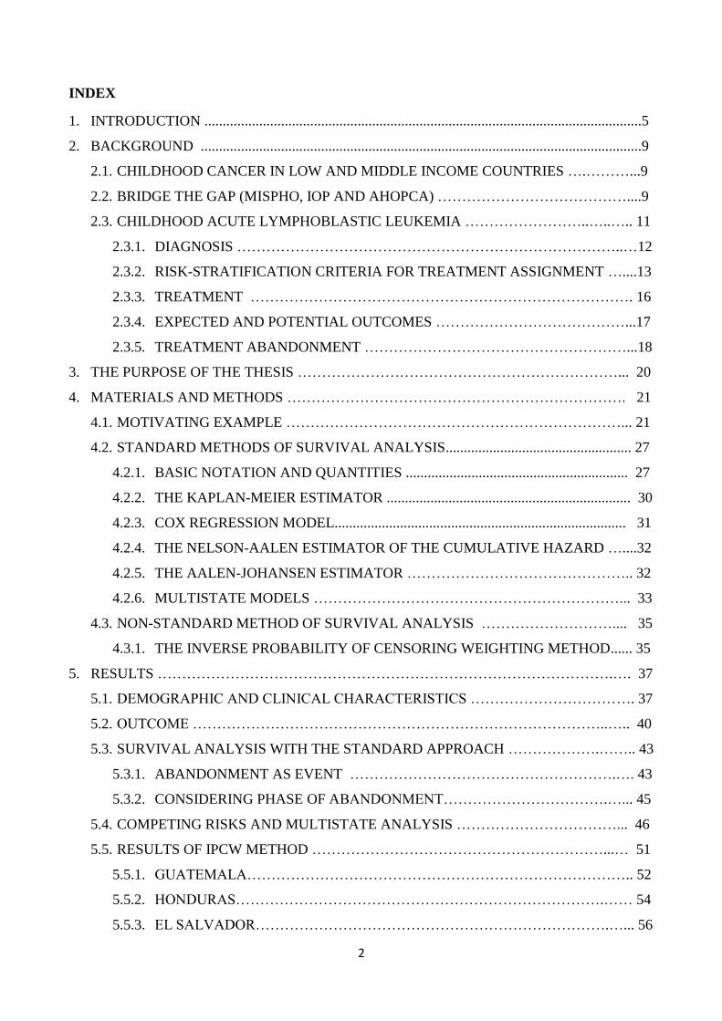
INDEX

1. INTRODUCTION ........................................................................................................................5

2. BACKGROUND .........................................................................................................................9

2.1. CHILDHOOD CANCER IN LOW AND MIDDLE INCOME COUNTRIES ….………...9

2.2. BRIDGE THE GAP (MISPHO, IOP AND AHOPCA) …………………………………....9

2.3. CHILDHOOD ACUTE LYMPHOBLASTIC LEUKEMIA ……………………..…..….. 11

2.3.1. DIAGNOSIS ……………………………………………………………………..…12

2.3.2. RISK-STRATIFICATION CRITERIA FOR TREATMENT ASSIGNMENT …....13

2.3.3. TREATMENT ……………………………………………………………………. 16

2.3.4. EXPECTED AND POTENTIAL OUTCOMES …………………………………...17

2.3.5. TREATMENT ABANDONMENT ………………………………………………...18

3. THE PURPOSE OF THE THESIS …………………………………………………………... 20

4. MATERIALS AND METHODS ……………………………………………………………. 21

4.1. MOTIVATING EXAMPLE ……………………………………………………………... 21

4.2. STANDARD METHODS OF SURVIVAL ANALYSIS................................................... 27

4.2.1. BASIC NOTATION AND QUANTITIES ............................................................. 27

4.2.2. THE KAPLAN-MEIER ESTIMATOR ................................................................... 30

4.2.3. COX REGRESSION MODEL................................................................................ 31

4.2.4. THE NELSON-AALEN ESTIMATOR OF THE CUMULATIVE HAZARD …....32

4.2.5. THE AALEN-JOHANSEN ESTIMATOR ……………………………………….. 32

4.2.6. MULTISTATE MODELS ………………………………………………………... 33

4.3. NON-STANDARD METHOD OF SURVIVAL ANALYSIS ……………………….... 35

4.3.1. THE INVERSE PROBABILITY OF CENSORING WEIGHTING METHOD...... 35

5. RESULTS ………………………………………………………………………………….…. 37

5.1. DEMOGRAPHIC AND CLINICAL CHARACTERISTICS ……………………………. 37

5.2. OUTCOME …………………………………………………………………………..….. 40

5.3. SURVIVAL ANALYSIS WITH THE STANDARD APPROACH ……………….…….. 43

5.3.1. ABANDONMENT AS EVENT ……………………………………………….…. 43

5.3.2. CONSIDERING PHASE OF ABANDONMENT…………………………….…... 45

5.4. COMPETING RISKS AND MULTISTATE ANALYSIS ……………………………... 46

5.5. RESULTS OF IPCW METHOD ……………………………………………………...… 51

5.5.1. GUATEMALA…………………………………………………………………….. 52

5.5.2. HONDURAS………………………………………………………………….…… 54

5.5.3. EL SALVADOR……………………………………………………………….…... 56

3

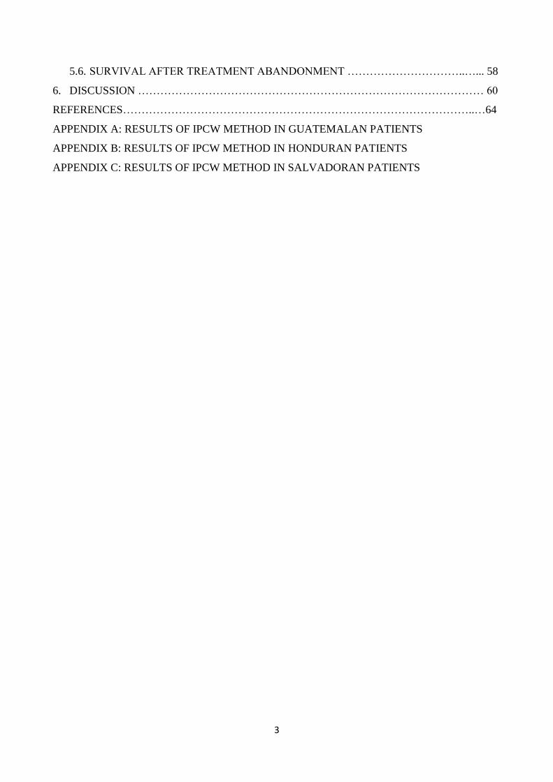
5.6. SURVIVAL AFTER TREATMENT ABANDONMENT …………………………..…... 58

6. DISCUSSION ………………………………………………………………………………… 60

REFERENCES…………………………………………………………………………………..…64

APPENDIX A: RESULTS OF IPCW METHOD IN GUATEMALAN PATIENTS

APPENDIX B: RESULTS OF IPCW METHOD IN HONDURAN PATIENTS

APPENDIX C: RESULTS OF IPCW METHOD IN SALVADORAN PATIENTS

4

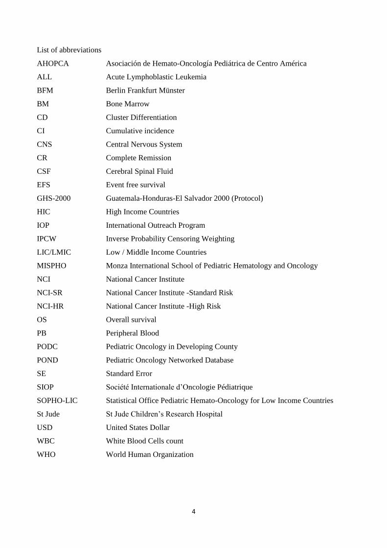
List of abbreviations

AHOPCA Asociación de Hemato-Oncología Pediátrica de Centro América

ALL Acute Lymphoblastic Leukemia

BFM Berlin Frankfurt Münster

BM Bone Marrow

CD Cluster Differentiation

CI Cumulative incidence

CNS Central Nervous System

CR Complete Remission

CSF Cerebral Spinal Fluid

EFS Event free survival

GHS-2000 Guatemala-Honduras-El Salvador 2000 (Protocol)

HIC High Income Countries

IOP International Outreach Program

IPCW Inverse Probability Censoring Weighting

LIC/LMIC Low / Middle Income Countries

MISPHO Monza International School of Pediatric Hematology and Oncology

NCI National Cancer Institute

NCI-SR National Cancer Institute -Standard Risk

NCI-HR National Cancer Institute -High Risk

OS Overall survival

PB Peripheral Blood

PODC Pediatric Oncology in Developing County

POND Pediatric Oncology Networked Database

SE Standard Error

SIOP Société Internationale d’Oncologie Pédiatrique

SOPHO-LIC Statistical Office Pediatric Hemato-Oncology for Low Income Countries

St Jude St Jude Children’s Research Hospital

USD United States Dollar

WBC White Blood Cells count

WHO World Human Organization

5

1. INTRODUCTION

Childhood cancer is a worldwide public health concern being a leading cause of death in children.

While high-income countries have improved the probability of surviving after cancer diagnosed

in pediatric age (it now reaches 80%), children and adolescents with cancer living in low and

middle-income countries (LIC/LMIC) have a dismal outcome. This is due to many reasons,

including the lack of resources, scarce living conditions and the high priority for public health on

communicable diseases. The higher proportion of children in the populations of these countries

magnifies the problem. Thanks to the enthusiasm of the pediatric oncology community, many

initiatives have been implemented with the aim to improve survival after cancer in children in

LIC/LMIC.

One important initiative is the AHOPCA (Asociación de Hemato-Oncología Pediátrica de Centro

América) network, which is a group of hospital units specialized in childhood cancer treatment

from Central America and the Caribe. These countries faces common difficulties such as

widespread poverty (25 to 60% of their populations live below the poverty line), malnutrition,

illiteracy, poor infrastructure, difficult access to health services, inconsistent drug availability,

lack of supportive care and low priority of cancer treatment if compared to the priority of other

health issues (mostly infectious diseases).1–6

This network developed from an initial partnership (1986) between Manuel de Jesus “La

Mascota” Hospital (Managua, Nicaragua), and three institutions in Europe, the Pediatric Clinic

of the University of Milano-Bicocca (Monza, Italy). Followed by the San Giovanni Hospital in

Bellinzona (Switzerland) and the Istituto Nazionale di Tumori in Milan (Italy) that lead to the

establishment in the late 80ies of the Monza International School of Pediatric Hemato-Oncology

(MISPHO). In the same period (1994) St. Jude Children’s Research Hospital (Memphis, USA)

established a twinning program with the Hospital Benjamin Bloom (San Salvador, El Salvador),

in the framework of the International Outreach Program. Almost a decade later, after the

participation in MISPHO, and thanks to their geographical and linguistic proximity, the countries

of Central America joined formally into the AHOPCA collaborative group.1,7

Nowadays, the AHOPCA network promotes the development of shared clinical protocols (mainly

focused on cancer chemotherapy), educational programs for physicians and nurses, a more

integrated role for psychologist and social workers in the approach to patients and collaborative

research. A data management infrastructure has also been developed, the Pediatric Oncology

6

Networked Database (best known as POND), located at the St Jude and complemented by the

statistical support from a small team at the University of Milano-Bicocca named SOPHO-LIC

(Statistical Office Pediatric Hemato-Oncology in Low-Income Countries). This facilitates the

application of various treatment protocols, the collection of data on diagnosis, treatment and

outcome and the evaluation of the results achieved for children affected by cancer in these

countries. 2,4,8–14

In this context, survival analysis is the methodology typically used to describe the outcome in

cancer clinical trials and is also used as an indicator of their efficacy in disease management and

care. Survival analysis deals with the study of the time elapsed between some initial event defined

as a starting point (such as date of diagnosis or start of treatment) and the time of occurrence of

some event (failure) of interest (such as disease relapse or death).

A typical complexity of observed survival data is the presence of right censoring on the survival

time, which occurs generally when the survival time is shorter than the failure time. Censoring is

due to a limitation on the observability of the failure/survival time itself (for this reason it is called

administrative censoring) and has to be accounted for in the analysis. Statistical methods in

survival analysis were developed mostly to address for the presence of censoring and for the non-

symmetric shape of the distribution of survival time. In the classical survival analysis theory, the

censoring distribution is reasonably assumed to be independent of the survival time distribution,

i.e. censoring is non-informative on the “true” survival time. This assumption implies that the

velocity of occurrence of failure can be estimated by considering the survival experience of the

non-censored times.

In more complex situations, like treatment abandonment, censoring cannot be directly assumed

as independent from the survival experience (informative censoring). In this case, the issue is to

account for the information carried from the censoring time on the true survival time. The

censoring time could “hide” a survival time which would be observed right after the censoring

time if, for example, the patient decided deliberately to leave the treatment/study given his/her

very bad conditions and with a dismal prognosis. On the other hand, the censoring time could

“hide” a very long survival time if, for example, the patient decided deliberately to leave the

treatment/study when his/her conditions were very good and the disease apparently cured.

7

Treatment abandonment is a relevant problem in LIC/LMIC and, according to the experience of

these countries, some of the children who abandon treatment are seen later alive and in complete

remission, others return to the clinic with relapse or progressive disease or die, most of them do

not return, are not traced again and their status is unknown. Given these considerations, it is clear

that abandonment is not the standard administrative censoring and is not independent of the

survival experience.

Considering abandonment of therapy as an event (failure) likely leads to underestimate the

protocol effect but considering it as administrative censoring can lead to overestimate the effect.

In SIOP (Société Internationale d’Oncologie Pédiatrique) a PODC working groups (Pediatric

Oncology in Developing Country) recommended to carefully document every abandonment of

treatment and, with SOPHO-LIC, suggested to perform the estimation of EFS (event-free

survival) in two ways: by treating abandonment as a failure and by censoring.15

Several studies on the causes of abandonment of therapy in LIC demonstrated that is highly

related to patient’s socioeconomic condition, time travel for patients to the specialized clinic,

parent’s illiteracy, low monthly household income (less than 100 USD) and increased number of

household family members.16–19

Other studies conducted in LIC/LMIC revealed some other possible causes such as nutritional

status, hospital policies (financial burden of treatment) and other cultural aspects that are difficult

to document (such as beliefs, feelings, fears). Arora et al. summarized many probable causes and

possible solutions such as twinning programs, an increase of financial support, development of

adapted protocols to be delivered in specialized clinics, which actually are the measures adopted

from AHOPCA network.20–24

Thanks to these efforts the prevalence of abandonment has been reduced significantly in El

Salvador and Guatemala, where the rate in 2002 was less than 2%, while it remains higher than

10% in other countries (Honduras, Nicaragua).1,4,25 However, the problem is still present and,

given its nature, difficult to be completely solved.

This project aims at estimating the survival outcome of childhood cancer in LIC/LMIC countries

where treatment abandonment is a relevant issue with approaches that can deal with the

8

informative nature of the related censored information. The project will develop the following

two points:

1. Handling informative censoring on survival time due to the abandonment of treatment, using

the non-standard statistical method of Marginal Structural Model.

2. Comparing the classic with the non-standard statistical methods in evaluating the effects of

treatment protocols in children with of acute lymphoblastic leukemia treated in LIC/LMIC.

9

2. BACKGROUND

2.1. CHILDHOOD CANCER IN LOW AND MIDDLE-INCOME COUNTRIES

Childhood cancer is a worldwide public health concern. The incidence and mortality rates

differ from country to country, also depending on the how accuracy of reported data. World

Human Organization (WHO) estimates for childhood cancer (<15 years old) a worldwide

incidence rate of 8.8 per 100,000 per year and a mortality rate of 4.3 per 100,000 per year. 26

Möricke et al reported results of consecutive trials; children from HIC (Germany, Austria,

and Switzerland) were diagnosed with acute lymphoblastic leukemia, and treated according

to BFM-protocols; the 10-year event-free survival (EFS) was improved from 65% (SE =

0.02) for the ALL-BFM 81 study to a 10-year EFS of 78% (SE = 0.01) for the ALL-BFM 95

study.27 While Navarrete et al reported the results of the AHOPCA-ALL 2008 the estimated

3-year EFS was 59.4% (SE = 1.7)3, and Magrath et al reported a 4-year EFS of 45% (1986)

that improved to 61% in (1997) for one treatment center in India.28 This gap in survival is

due in part to treatment abandonment; as well as the shortage of chemotherapy agents, poor

living conditions, late diagnosis and difficult access to a prompt treatment, evidenced by

higher rates of mortality and relapse

2.2. BRIDGE THE GAP (MISPHO, IOP, AND AHOPCA)

One of the most encouraging successes in childhood cancer treatment is the improved

survival in developed countries among children with acute lymphoblastic leukemia (ALL)

that sees nowadays more than 80% survival at 5 years from diagnosis while the

corresponding figure was less than 50% in the 60ies. In order to bring these benefits to

children that live in LIC/LMIC cooperative efforts have been carried on and main strategies

comprehend:

-Twinning programs, professionals from institutions in HIC have collaborated with

their colleagues in LIC/LMIC. This has promoted the progress of pediatric oncology

care, though educational programs (for health workers such as physicians, nurses, and

others), development of tailored treatment protocols, implementation of cancer

registration and promotion of clinical research.

10

-Local sustainability, through the development of oncology units with the support of

the local governments and non-government foundations that facilitate the treatment of

pediatric cancer.4,5,25

These actions were implemented also in the AHOPCA network which was created in the

late 90ies after the experience with MISPHO and with the Outreach program of the St. Jude

Children’s Research Hospital.1,5,7

The countries that constitute the AHOPCA network are Guatemala, El Salvador, Honduras,

Nicaragua, Costa Rica, Panama, Dominican Republic and Haiti (that joined recently). The

network promotes the development of shared clinical protocols (mainly focused on cancer

chemotherapy), educational programs for physicians and nurses, and a more integrated role

for psychologist and social workers in clinical units and collaborative research.

A data management infrastructure has also been developed, after a MISPHO pilot program,

in collaboration with St Jude. POND, which became the main database. This online network

database has incorporated a software that allows real-time monitoring of patients outcomes,

shared protocols, and generation of chemotherapy roadmaps. It allows web-based data

reporting on diagnosis, treatment, and outcome and may be extended to include data on

supportive care, the health-related quality life of children affected by cancer in these

countries. 2,4,8–14

Along these years, there has been teamwork carried out between oncologists, their partners

of the twinning institutions (especially Monza and St. Jude), the data managers of the

AHOPCA network, the POND developers and the statisticians in SOPHO-LIC. This

teamwork has allowed: to develop tailored treatment protocols for various cancers; to collect

the data and to report data and discuss results on treatment efficacy to the regular annual

meetings of AHOPCA.4,13

11

2.3. CHILDHOOD ACUTE LYMPHOBLASTIC LEUKEMIA

The WHO estimates for childhood acute leukemia (<15 years old) a worldwide incidence

rate of 2.7 per 100,000 per year and a mortality rate of 1.5 per 100,000 per year. Moreover,

for the countries of the AHOPCA network, it estimates an incidence rate of 2.9 per 100,000

per year and a mortality rate of 1.9 per 100,000 per year. 26 Leukemia, overall these countries,

constitutes approximately 30% of incident childhood cancers.

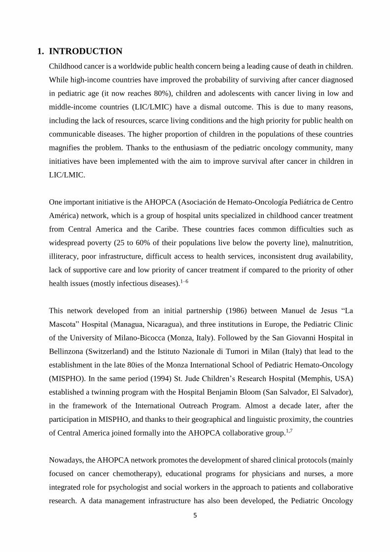
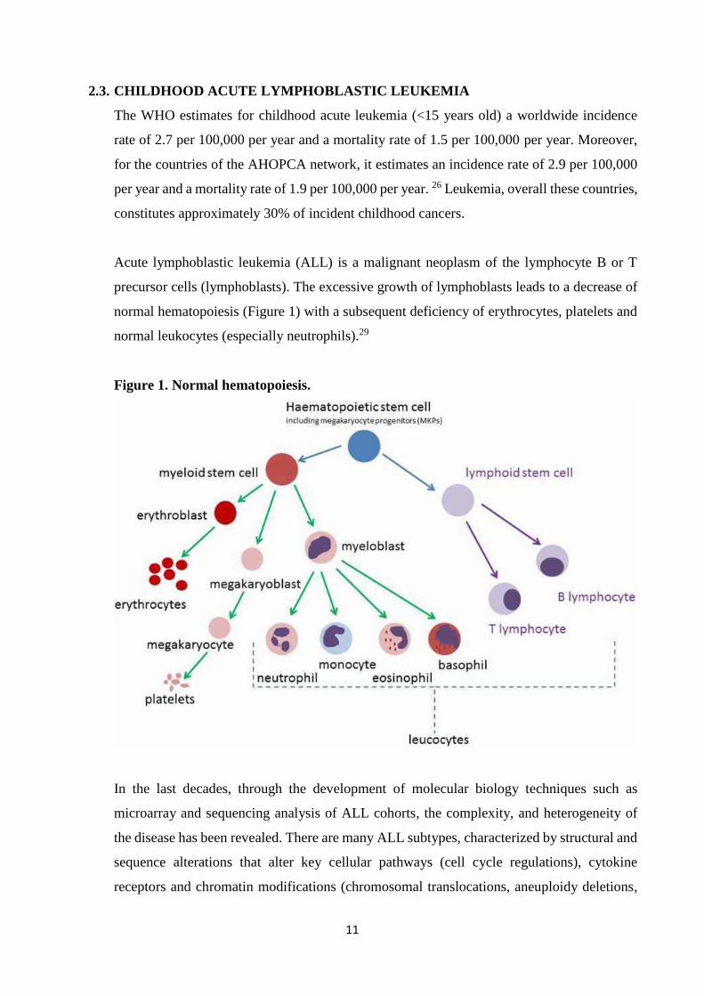
Acute lymphoblastic leukemia (ALL) is a malignant neoplasm of the lymphocyte B or T

precursor cells (lymphoblasts). The excessive growth of lymphoblasts leads to a decrease of

normal hematopoiesis (Figure 1) with a subsequent deficiency of erythrocytes, platelets and

normal leukocytes (especially neutrophils).29

Figure 1. Normal hematopoiesis.

In the last decades, through the development of molecular biology techniques such as

microarray and sequencing analysis of ALL cohorts, the complexity, and heterogeneity of

the disease has been revealed. There are many ALL subtypes, characterized by structural and

sequence alterations that alter key cellular pathways (cell cycle regulations), cytokine

receptors and chromatin modifications (chromosomal translocations, aneuploidy deletions,

12

and amplifications). 30,31 Although etiology remains unclear, some possible etiologic risk

factors are genetic, infectious diseases, radiation, and/or chemical exposures.29

2.3.1. DIAGNOSIS

Initial clinical presentation depends on the infiltration of ALL cells into tissues. Virtually any

organ system may be involved, but peripheral blood, lymph nodes, spleen, liver, central

nervous system (CNS) and skin are the most common sites clinically detected. Patients often

present a short history of fatigue, lethargy, weight loss, bone pain, fever and/or spontaneous

bleeding. When CNS is involved, clinical presentation can include nausea, vomiting,

headache, neuropathies and papilledema. Testicular involvement is usually a painless

unilateral mass noted at diagnosis. The physical exam often reveals pallor, lymphadenopathy,

splenomegaly, hepatomegaly and signs associated with thrombocytopenia (gingival

bleeding, epistaxis, petechiae/ecchymosis).29

The initial diagnosis of ALL includes peripheral blood cell count (WBC) with differential

hemogram, cytomorphological examination of bone marrow (BM) and cerebrospinal fluid

(CSF). With the presence of lymphoblasts in peripheral blood (PB) and/or their presence (≥

25%) in the bone marrow. ALL can be diagnosed with an appropriate stained of PB or BM,

preferably, with May-Grünwald-Giemsa. The French-American-British (FAB) scoring

system considers (1) the nuclear/cytoplasmic ratio; (2) the presence, prominence and

frequency of nucleoli; (3) the nuclear shape and (4) the cell size to classify ALL in two basic

subtypes L1 and L2, these subtypes are more descriptive than specific, but still used when

immunophenotyping is not available.32,33

Nowadays classification of ALL is based on immunophenotyping by flow cytometry and

genotype. Phenotypic evaluations comprehend cytochemical studies such as

myeloperoxidase (MPO) or Sudan black B reaction and specific esterase reactions to exclude

most cases of acute myeloid leukemia. Additional detection of surface and cytoplasmic

markers by flow cytometry identifies the leukemic cell population through monoclonal

antibodies identified as Clusters of Differentiation (CD). The commonly used markers for

immunophenotyping in acute leukemia are: (1) General, CD34, Human leukocyte Antigen-

D Related (HLA-DR), terminal deoxynucleotidyl transferase (TdT), CD45; (2) B-cell

markers, CD10, CD19, cCD22, CD20, cCD79A, CD24, c and sIg and (3) T-cell markers,

CD1a, CD2, cCD3, CD4, CD5, CD7, and CD8. 29,34

13

Once the ALL diagnosis is established, other complementary genetic studies such as

karyotyping and detection of chromosomal rearrangements are helpful to define features that

have prognostic value. Karyotyping detects gross chromosomal alterations in B-cell

precursor ALL (B-ALL), hyperdiploidy (>50 chromosomes, occurs in 25-30% of childhood

B-ALL) is associated with favorable outcome and hypodiploidy (<44 chromosomes, occurs

in 2-3% of childhood B-ALL) is associated with poor outcome. The chromosomal

rearrangements create chimeric fusion genes that commonly involve hematopoietic

transcription factors, epigenetic modifiers, cytokine receptors and tyrosine kinases. Common

B-ALL rearrangements are the t(12;21)(p13;q22) encoding ETV6-RUNX1 (TEL-AML),

t(1;19)(q23;13) encoding TCF3-PBX1 (E2A-PBX1), t(9;22)(q34;q11.2) encoding BCR-ABL1

(“Philadelphia” chromosome) and t(4;11)(q21;q23) encoding MLL-AF4 fusion; another key

genetic alterations are PAX5, IKZF1, JAK1/2 and CRLF2. T-cell precursor ALL (T-ALL) is

characterized by mutations of NOTCH1 and rearrangements of transcription factors TLX1

(HOX11), TLX3 (HOX11L2), LYL1, TAL1, and MLL.31

Initial assessment of CSF at diagnosis is essential for diagnosis and staging, it comprehends

CSF-chemistry (protein and glucose), the cell count of nucleated cells and erythrocytes (in a

counting chamber) and the cell morphology assessment on a high-quality cytospin

preparation. For patients with neurological symptoms, a careful evaluation accomplished

with cranial imaging by axial tomography (CT) o magnetic resonance (MRI) is mandatory.29

2.3.2. RISK-STRATIFICATION CRITERIA FOR TREATMENT ASSIGNMENT

The intensity of treatment is tailored to the prognostic profile of the patients as defined by

clinical and biological features. Patients who are likely to have good prognosis receive a less

intensive therapy, patients with high-risk features will receive more aggressive and

potentially more toxic treatment due to their lower probability of long-term survival.

The National Cancer Institute (NCI) risk stratification criteria is commonly use, to classify

B-cell ALL into Standard risk (WBC count <50,000/l and age 1 to younger than 10 years)

and High risk (WBC count ≥50,000/l and/or age 10 years or older).35 However,

stratification criteria should take into account all available characteristics to assign treatment

risk. For children with ALL the factors that have demonstrated prognostic value are

summarized below:

14

Patient and clinical disease characteristics:

Age at diagnosis, patients aged at least 1 but younger than 10 years have usually

reported a better long-term survival than older children (≥10 years old), adolescents

and, than infants (<1-year-old).

White blood cell count at diagnosis, 50,000/l is used as a cut point between better

and poorer prognosis, although the relationship between WBC count and the

prognosis is more complex and survival tend to be poorer at increasing WBC count.

CNS involvement, patients who have a non-traumatic diagnostic lumbar puncture may

be placed into CNS 1 (CSF with cytospin negative for blasts regardless of WBC

count), CNS 2 (CSF with <5 WBC/L and cytospin positive for blasts) or CNS 3

(CSF with ≥5 WBC/L and cytospin positive for blasts). Patients with CNS 3 and

patients with a traumatic puncture (≥10 erythrocytes/L) that include blasts have a

higher risk of CNS relapse and overall poorer outcome.36

Testicular involvement, in early ALL trials, was considered an adverse prognostic

factor. With more intensive induction therapy, it does not appear to have prognostic

significance.37

Down syndrome (trisomy 21), some studies report lower survival probability for these

patients, due in part to an increased treatment-related mortality and higher rates of

induction failure.38

Gender, some studies report better prognosis for girls than for boys with ALL, one

reason is the occurrence of testicular relapses.39

Race and ethnicity, survival rates in black and Hispanic children with ALL are lower

than in white and Asian children with ALL. Associated factors are ALL subtypes

(black children have a higher rate of T-cell), ancestry related genomic variations (e.g.

polymorphisms of the ARID5B more frequent in Hispanics) and lower adherence to

treatment (mostly in Hispanic children).40,41

15

Leukemic characteristics:

Immunophenotype, precursor B-lymphoblastic leukemia (distinguished from mature

B-cell ALL –Burkitt) can be subdivided into Common precursor B (CD10 positive

and no surface of cytoplasmic Ig), Pro-B (CD10 negative) and Pre-B (presence of

cytoplasmic Ig). Patients with common precursor B-cell ALL usually are associated

with favorable cytogenetic. Instead, the absence of CD10 is associated with MLL gene

rearrangements and the presence of cytoplasmic Ig is associated with TXF3-PBX1

fusion, both with a poorer prognosis. T-cell ALL with appropriately intensive therapy

has an outcome similar that of B-cell ALL. Some translocations have been identified

in T-cell ALL, high expression of TLX1/HOX11 is associated with more favorable

outcome and TLX3/HOX11L2 appears to be associated with increased risk of

treatment failure. Myeloid antigen expression can be found and it could be associated

with MLL rearrangements and ETV6-RUNX1 gene rearrangement, but no independent

adverse prognostic significance has been found.42

Cytogenetic and genomic alterations, chromosomal abnormalities have been shown

to have prognostic significance, especially in precursor B-cell ALL. High

hyperdiploidy (51-65 chromosomes) and ETV6-RUNX1 fusion are associated with

favorable outcomes. Others have been associated with poorer prognosis, including

Philadelphia chromosome (t(9;22)(q34;q11.2)), MLL rearrangements, hypodiploidy

and intrachromosomal amplification of the AML1 gene (iAMP21). Also, a number of

polymorphisms of genes, such as NUDT15, involved in the metabolism of

chemotherapeutic agents have been reported as prognostic factors in childhood

ALL.42

Response to initial treatment:

Cytomorphological evaluation in BM and PB, evaluate the clearance of the tumor

burden in the initial phase of treatment has been shown to be an important prognostic

factor. Specifically, the absolute blast count in PB on day 8 (Prednisone response)27

and the percentage of blasts in the BM identifies the good or poor response to

treatment, and are currently used in ALL protocols to define prognosis.43

Minimal residual disease determination (MRD), is the accurate and sensitive

detection of low frequencies of ALL cells (≤1 ALL cell in 10000 normal cells) in

16

blood and BM by flow cytometry or polymerase chain reaction (PCR)- based

molecular techniques.44

2.3.3. TREATMENT

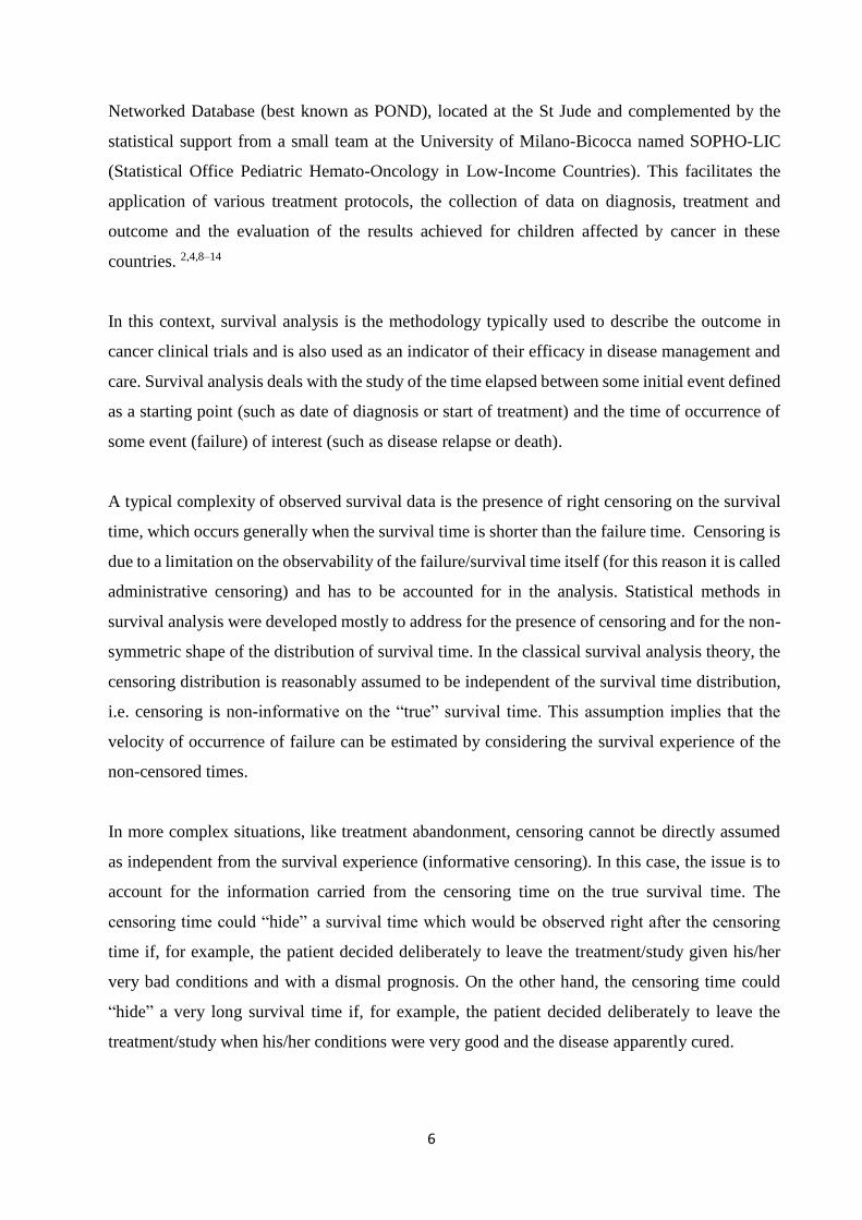
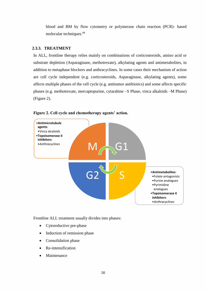
In ALL, frontline therapy relies mainly on combinations of corticosteroids, amino acid or

substrate depletion (Asparaginase, methotrexate), alkylating agents and antimetabolites, in

addition to metaphase blockers and anthracyclines. In some cases their mechanism of action

are cell cycle independent (e.g. corticosteroids, Asparaginase, alkylating agents), some

affects multiple phases of the cell cycle (e.g. antitumor antibiotics) and some affects specific

phases (e.g. methotrexate, mercaptopurine, cytarabine –S Phase, vinca alkaloids –M Phase)

(Figure 2).

Figure 2. Cell cycle and chemotherapy agents’ action.

Frontline ALL treatment usually divides into phases:

Cytoreductive pre-phase

Induction of remission phase

Consolidation phase

Re-intensification

Maintenance

•Antimetabolites:•Folate antagonists•Purine analogues•Pyrimidine analogues

•Topoisomerase II inhibitors:•Anthracyclines

•Antimicrotubule agents:

•Vinca alcaloids

•Topoisomerase II inhibitors:

•Anthracyclines M G1

SG2

17

Along with CNS directed treatment (intrathecal therapy) and radiotherapy when

needed

The cytoreductive pre-phase (typically BFM-oriented protocols) consists of one week of

corticosteroids (prednisone or dexamethasone) and one dose intrathecal methotrexate.

Patients usually present with hyperleukocytosis (WBC count ≥50,000/l) and/or tumor lysis

syndrome which implies a comprehensive initial treatment (such as this pre-phase). The

evaluation of the clearance of peripheral blasts at the end of this phase has been identified as

an important prognostic factor.

Through decades with the introduction of diverse chemotherapeutic agents, induction to

remission phase has been developed. With the combination of corticosteroids, vinca

alkaloids, Asparaginase, intrathecal methotrexate, and anthracyclines most of the patients

achieve remission (the disappearance of all signs of cancer). Next phases (consolidation, re-

induction, and maintenance –the less intensive phase) vary according to risk stratification

and between protocols and are designed and administered to maintain continuous complete

remission and prevent relapse. ALL treatment protocols are designed to last 2 years (or up to

3 years in certain protocols/subgroups).

The clinical research allowed the development of other therapies, especially for patients with

poor prognosis, such as allogeneic hematopoietic stem cell transplantation (HSTC), specific

inhibitors for selective pathways and novel immunotherapeutic approaches that intend to be

adaptive and improve the expected survival in the presence of specific biological features.

2.3.4. EXPECTED AND POTENTIAL OUTCOMES

The first goal of any regimen is to attain complete remission (CR) followed by a long-term

survival. For ALL CR is defined as the disappearance of all the signs of the disease, in the

bone marrow (<5% blast cells –M1– with sufficient cellularity and signs of regeneration of

normal myelopoiesis), in the CSF and any other sites that were infiltrated at the diagnosis.

With an appropriate adherence to current regimens approximately 98% of children with ALL

achieve CR 45 .

The events that may occur as treatment failures are first of all the lack of CR due to death

during induction or the resistance to treatment. In patients who experience CR, the events

18

that may occur are a relapse, death or the diagnosis of a second malignant neoplasm either

during treatment or after the end of therapy during clinical follow-up. (See section 4 for the

detailed definition).

2.3.5. TREATMENT ABANDONMENT

The occurrence of treatment abandonment, as often observed in LIC/LMIC, is of major

concern because it prevents the correct administration of the full treatment regimen to the

child with cancer and affects the effectiveness of the treatment and prevents observing the

patient’s next/final state. It is defined as the termination of the relationship between the

patient and the treatment center during active therapy. The current more specific definition

of abandonment of treatment for AHOPCA is missing four or more consecutive scheduled

weekly visits during active treatment. 3,4,13,14

Several studies on the causes of treatment abandonment in LIC demonstrated that is highly

related to patient’s socioeconomic condition. Metzger et al. assessed the outcome of ALL

pediatric patients in Honduras; they found that the main cause of failure was treatment

abandonment (23%). The Gray’s proportional hazard model showed that it was associated

with prolonged travel time to the treatment center at Tegucigalpa (> 2 hours) and to a patient’s

younger age (< 4.5 years). To address the problem of travel time, in 2002 a satellite clinic in

the second largest city in the country (San Pedro Sula) was set up and results of this policy

are now being investigated.16

Bonilla et al. assessed the prevalence and predictors of treatment abandon in cancer patients

(diagnosed with leukemia, lymphoma and solid tumors) from El Salvador. They reported that

the prevalence of treatment abandonment was of 13%, occurring at a median time of 2 months

(from the beginning of therapy) and that it was associated with parent’s illiteracy, low

monthly household income (less than 100 USD) and increased number of household family

members.17

Sweet-Cordero et al. assessed predictors of treatment abandon in children with cancer in

Guatemala; they evaluated economic, family and community factors through a questionnaire.

They found that less than 3 years of elementary school paternal education were strongly

associated to treatment abandon. Meanwhile, access to mainstream and strong family support

19

were associated with adherence to treatment.18 An instrument was developed to assess socio-

economic status of the cancer patient’s family in order to support them accordingly.19

Other studies conducted in diverse LIC/LMIC revealed some other possible causes such as

nutritional status, hospital policies (financial burden of treatment) and other cultural aspects

that are difficult to document.20–24

20

3. THE PURPOSE OF THIS THESIS

The project will develop the following two points:

1) Handling informative censoring on survival time due to the abandonment of treatment, using

the non-standard statistical method of Marginal Structural Model, in order to obtain an

unbiased estimate of the outcome.

2) Comparing the classic with the non-standard statistical methods in evaluating the outcome of

treatment protocols of acute lymphoblastic leukemia in low-income countries.

21

4. MATERIALS AND METHODS

4.1. MOTIVATING EXAMPLE

The protocols to treat ALL shared in the AHOPCA network are based on the St Jude and

AIEOP-BFM experiences and tailored according to local resources (usually chemotherapy

intensity has to be reduced).

For the purpose of this investigation we focused on the results from Guatemala, El Salvador,

and Honduras, because the ALL treatment protocols have been shared since February 2000:

In the first shared experience, ALL patients were treated according to the protocol

denominated GHS-2000 based on the protocol Total XI and Total XIIIB developed by St

Jude Children’s Research Hospital.

The second experience consists of the protocols AHOPCA ALL-2008 (El Salvador and

Honduras), and LLAG-0707 (Guatemala), both based on the ALL-IBC-BFM 2002 of the

International Berlin-Frankfurt-Münster Study Group (BFM).

PATIENTS:

The protocols were designed to treat children and adolescents between 1-17 years old (some

infants were included), newly diagnosed with ALL, and with the informed consent of parents

or legal guardians. Patients previously treated were excluded. The diagnosis of ALL was

based on a morphological assessment of May-Grünwald or modified Giemsa-stained smears

of bone marrow and immunophenotyping was performed by flow cytometry with a basic

panel. Clinical examination, WBC count, CNS assessment and complementary studies were

also performed.

RESPONSE AND EVENTS DEFINITIONS:

Prednisone response: for BFM based protocol is performed on day 8 after receiving 7 days

of prednisone and one intrathecal dose of methotrexate (MTX). The presence in the

peripheral blood of less than 1,000 blasts/mm3 defines a good response (PGR) and having at

least 1,000 blasts/mm3 constitutes a poor response (PPR).

Bone marrow assessment: both protocols contemplate the morphological evaluation of the

bone marrow (BM) on day 15 and at the end of induction phase (day 36 or 33 according to

22

each protocol definitions). For BFM based protocols, patients who did not experience

complete remission by day 33 were evaluated after phase IB of the study or after the

subsequent high-risk (HR) blocks (for LLAG-0707 only). Bone marrow status was

categorized as M1 (<5% blasts), M2 (5-24% blasts) or M3 (≥25% blasts).

Complete remission (CR): was defined as M1 BM status with normal peripheral counts and

no extramedullary disease at the end of the induction/consolidative phase (according to each

protocol definitions).

Resistant disease: was defined as not experiencing CR after completing the

induction/consolidative phase of treatment (according to each protocol definitions).

Relapse: was defined as the reappearance of at least 25% blast in BM and/or extramedullary

disease after experiencing CR.

Death: event reported as death in induction (if it occurs during induction to remission phase,

before evaluating the remission status) and death in continuous CR due to treatment toxicity

(if occurs after achieving CR and the patient is in continuous in CR). Death can also occur

after another event such as resistant disease or relapse due to disease progression or related

to treatment.

Treatment abandonment: defined as missing 4 or more consecutive weekly scheduled visits

during therapy, reported as abandonment in induction (if occurs during induction to remission

phase –the patient left before achieving CR) and abandonment in CR (if occurs after

achieving CR).

Secondary Neoplasm Malignant (SNM): defined as the diagnosis of another malignant

neoplasm confirmed by pathology. It may occur during active treatment or, more commonly,

at long-term during follow-up.

23

RISK STRATIFICATION CRITERIA:

Considering the available information for all the patients for the following analysis, the

baseline risk was calculated according to the NCI risk stratification criteria. According to this

the Standard risk (or NCI-SR) comprehends patients between 1 to 10 years, B-linage and

with an initial white blood cell count (WBC) <50,000/mm3, while the High risk (or NCI-HR)

comprehend the rest of the patients.

CNS classification: CNS 1 (cerebrospinal fluid [CSF] without blasts and nontraumatic); CNS

2 (CSF with no more than 5 cells/mm3 with blasts or the spinal tap was traumatic [>10 red

blood cells/mm3] or performed more than 72 h after the beginning of therapy); CNS 3 (CSF

> 5 cells/mm3 with blasts or cerebral nerve palsy or a cerebral mass).

For GHS-2000 protocol, patients aged at least 1 year but younger than 10 years, a WBC count

of less than 50,000/mm3, B-lineage, hyperdiploidy (DNA index ≥ 1.6 and <1.6), no CNS 3

or testicular involvement, BM M1 on day 15 and 36 were considered Standard risk (SR), and

the rest of patients were considered High risk (HR).

For BFM-based protocols, patients aged at least 1 year but younger than 6 years, a WBC

count of less than 20,000/mm3, B-lineage, no CNS 3 or testicular involvement, BM M1 or

M2 on day 15, and no HR criteria were considered SR. High risk criteria were: patients aged

less than 1 year, PPR, BM M3 on day 15, no CR at day 33, the presence of t(9;22) or t(4;11)

positive, hypodiploidy (DNA index < 0·81) and, for AHOPCA ALL-2008, T-lineage.

Patients aged at least 6 years or having WBC count of at least 20,000/mm3 and no HR criteria

were considered Intermediate risk (IR). For ALLG-0707 T-lineage and SR patients with BM

M3 on day 15, with no HR criteria were also considered IR.

24

TREATMENT:

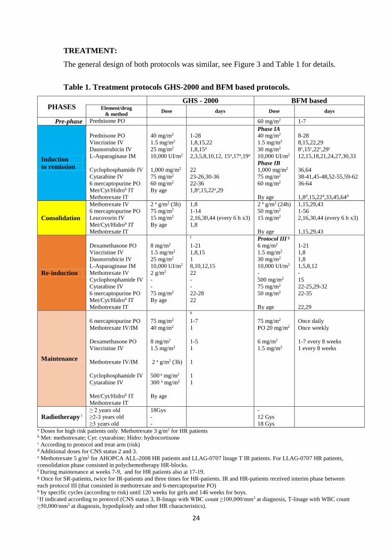
The general design of both protocols was similar, see Figure 3 and Table 1 for details.

Table 1. Treatment protocols GHS-2000 and BFM based protocols.

PHASES GHS - 2000 BFM based

Element/drug

& method Dose days Dose days

Pre-phase Prednisone PO 60 mg/m2 1-7

Induction

to remission

Prednisone PO

Vincristine IV

Daunorrubicin IV

L-Asparaginase IM

Cyclophosphamide IV

Cytarabine IV

6 mercaptopurine PO

Met/Cyt/Hidrob IT

Methotrexate IT

40 mg/m2

1.5 mg/m2

25 mg/m2

10,000 UI/m2

1,000 mg/m2

75 mg/m2

60 mg/m2

By age

1-28

1,8,15,22

1,8,15a

2,3,5,8,10,12, 15a,17a,19a

22

23-26,30-36

22-36

1,8a,15,22a,29

Phase IA

40 mg/m2

1.5 mg/m2

30 mg/m2

10,000 UI/m2

Phase IB

1,000 mg/m2

75 mg/m2

60 mg/m2

By age

8-28

8,15,22,29

8c,15c,22c,29c

12,15,18,21,24,27,30,33

36,64

38-41,45-48,52-55,59-62

36-64

1,8d,15,22d,33,45,64d

Consolidation

Methotrexate IV

6 mercaptopurine PO

Leucovorin IV

Met/Cyt/Hidrob IT

Methotrexate IT

2 a g/m2 (3h)

75 mg/m2

15 mg/m2

By age

1,8

1-14

2,16,30,44 (every 6 h x3)

1,8

2 e g/m2 (24h)

50 mg/m2

15 mg/m2

By age

1,15,29,43

1-56

2,16,30,44 (every 6 h x3)

1,15,29,43

Re-induction

Dexamethasone PO

Vincristine IV

Daunorrubicin IV

L-Asparaginase IM

Methotrexate IV

Cyclophosphamide IV

Cytarabine IV

6 mercaptopurine PO

Met/Cyt/Hidrob IT

Methotrexate IT

8 mg/m2

1.5 mg/m2

25 mg/m2

10,000 UI/m2

2 g/m2

-

-

75 mg/m2

By age

f

1-21

1,8,15

1

8,10,12,15

22

-

-

22-28

22

Protocol III g

6 mg/m2

1.5 mg/m2

30 mg/m2

10,000 UI/m2

-

500 mg/m2

75 mg/m2

50 mg/m2

By age

1-21

1,8

1,8

1,5,8,12

-

15

22-25,29-32

22-35

22,29

Maintenance

6 mercaptopurine PO

Methotrexate IV/IM

Dexamethasone PO

Vincristine IV

Methotrexate IV/IM

Cyclophosphamide IV

Cytarabine IV

Met/Cyt/Hidrob IT

Methotrexate IT

75 mg/m2

40 mg/m2

8 mg/m2

1.5 mg/m2

2 a g/m2 (3h)

500 a mg/m2

300 a mg/m2

By age

h

1-7

1

1-5

1

1

1

1

75 mg/m2

PO 20 mg/m2

6 mg/m2

1.5 mg/m2

Once daily

Once weekly

1-7 every 8 weeks

1 every 8 weeks

Radiotherapy i ≥ 2 years old

≥2-3 years old

≥3 years old

18Gys

-

-

-

12 Gys

18 Gys

a Doses for high risk patients only. Methotrexate 3 g/m2 for HR patients b Met: methotrexate; Cyt: cytarabine; Hidro: hydrocortisone c According to protocol and treat arm (risk) d Additional doses for CNS status 2 and 3. e Methotrexate 5 g/m2 for AHOPCA ALL-2008 HR patients and LLAG-0707 linage T IR patients. For LLAG-0707 HR patients,

consolidation phase consisted in polychemotherapy HR-blocks. f During maintenance at weeks 7-9, and for HR patients also at 17-19. g Once for SR-patients, twice for IR-patients and three times for HR-patients. IR and HR-patients received interim phase between

each protocol III (that consisted in methotrexate and 6-mercaptopurine PO) h by specific cycles (according to risk) until 120 weeks for girls and 146 weeks for boys. i If indicated according to protocol (CNS status 3, B-linage with WBC count ≥100,000/mm3 at diagnosis, T-linage with WBC count

≥50,000/mm3 at diagnosis, hypodiploidy and other HR characteristics).

25

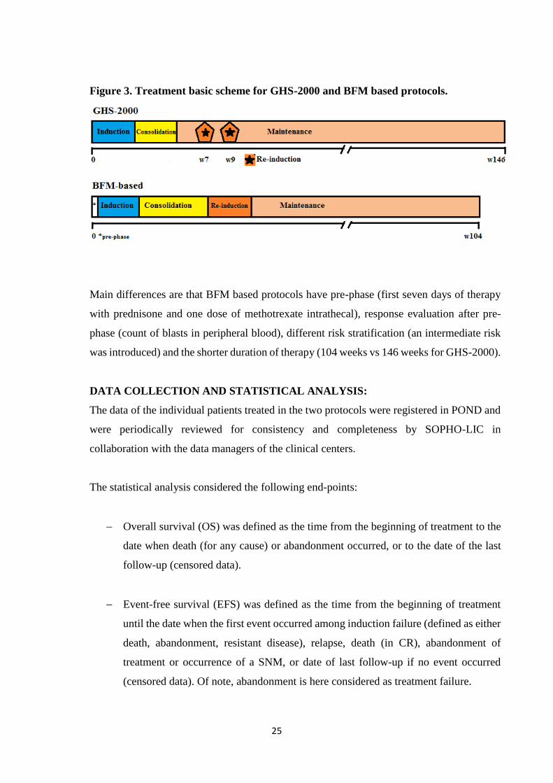
Figure 3. Treatment basic scheme for GHS-2000 and BFM based protocols.

Main differences are that BFM based protocols have pre-phase (first seven days of therapy

with prednisone and one dose of methotrexate intrathecal), response evaluation after pre-

phase (count of blasts in peripheral blood), different risk stratification (an intermediate risk

was introduced) and the shorter duration of therapy (104 weeks vs 146 weeks for GHS-2000).

DATA COLLECTION AND STATISTICAL ANALYSIS:

The data of the individual patients treated in the two protocols were registered in POND and

were periodically reviewed for consistency and completeness by SOPHO-LIC in

collaboration with the data managers of the clinical centers.

The statistical analysis considered the following end-points:

Overall survival (OS) was defined as the time from the beginning of treatment to the

date when death (for any cause) or abandonment occurred, or to the date of the last

follow-up (censored data).

Event-free survival (EFS) was defined as the time from the beginning of treatment

until the date when the first event occurred among induction failure (defined as either

death, abandonment, resistant disease), relapse, death (in CR), abandonment of

treatment or occurrence of a SNM, or date of last follow-up if no event occurred

(censored data). Of note, abandonment is here considered as treatment failure.

26

An alternative approach consists in not considering abandonment as a failure in all outcome

indicators. This implies to assume that abandonment causes a censored observation which is

equivalent to the common right censoring (where we can assume independence from

survival).

The probabilities of OS and EFS were estimated using the Kaplan-Meier method with

Greenwood standard error (SE).

Competing causes of failure were defined considering resistant disease, relapse, death and

treatment abandonment (occurring as first event), as competing risks. Crude cumulative

incidences of each cause of failure were estimated using the Aalen-Johansen estimator.

27

4.2. STANDARD METHODS FOR SURVIVAL ANALYSIS

4.2.1. BASIC NOTATION AND QUANTITIES

In general terms, survival analysis collects statistical procedures for which the Outcome

variable of interest is Survival time. This time variable gives the elapsed time between the

starting point (e.g. beginning of the relevant observation due to diagnosis, or treatment start,

or achievement of CR, etc.) until the occurrence of the event of interest. This Time could be

measured in years, months, weeks or days. The Event (also known as failure if it is negative),

could be death, relapse from remission, recovery or any designated experience of interest that

may happen to an individual. Sometimes more than one event is considered defining a

Composite Event. When analyzing the single events defining the composite events, the

correct approach is to adjust for Competing risks.

Censoring is a key analytical problem present in survival data and it is handled by any

statistical technique of the entire survival analysis theory. In practice, censoring occurs when

we do not know the exact time to the event, but we only know that this time is greater than

the censoring time. Censoring acts as a limitation on the observability of the event and thus

of the true survival time.

The most common reasons of right censoring are:

The study ends before a person experiences the event.

A person is lost to follow-up during the study period.

A person deliberately withdraws the treatment (drop out or treatment abandon).

A person is obliged to withdraw the treatment (e.g. due to an adverse reaction).

Some basic notations:

The random variable T denotes the non-negative survival time.

The scalar t denotes a generic nonnegative time instant; if we are interested in

evaluating a specific period of survival from some point t onwards the notation T>t is

used.

The Greek letter δ denotes the status indicator. It is set equal to 1 is the event was

observed or 0 if the time was censored.

The random variable ε denotes the event type indicator when in the presence of

competing risks. For instance, if the survival time may occur due to two different

causes of failure, ε = 1,2 represents the types of failure.

28

Z and Z denote a single or a vector of (fixed) covariates.

The survival function:

𝑺(𝒕) = 𝑃𝑟{𝑇 > 𝑡}

Gives the probability that a person survives in time (not failing) longer than any specified

time t. It is a fundamental quantity showing in time the fraction of subjects free from failure.

Theoretically S(0) = 1, because at the beginning of the study all subjects are free from failure

yet, and S(∞) = 0, because eventually, nobody would survive.

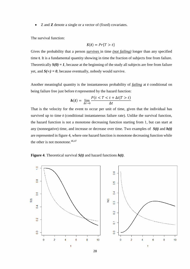
Another meaningful quantity is the instantaneous probability of failing at t conditional on

being failure free just before t represented by the hazard function:

𝒉(𝒕) = limΔ𝑡→0

𝑃(𝑡 < 𝑇 < 𝑡 + ∆𝑡|𝑇 > 𝑡)

∆𝑡

That is the velocity for the event to occur per unit of time, given that the individual has

survived up to time t (conditional instantaneous failure rate). Unlike the survival function,

the hazard function is not a monotone decreasing function starting from 1, but can start at

any (nonnegative) time, and increase or decrease over time. Two examples of S(t) and h(t)

are represented in figure 4, where one hazard function is monotone decreasing function while

the other is not monotone.46,47

Figure 4. Theoretical survival S(t) and hazard functions h(t).

29

While S(t) describes the pragmatic survival experience in time, h(t) provides insight about

how the instantaneous rate of the event may change with age or with time elapsed from the

origin. The function h(t) is the vehicle by which mathematical modeling of survival data is

carried out. Survival models are, in fact, usually written in terms of the hazard function.

Clearly, there is a one-to-one relationship between S(t) and h(t):

𝑺(𝒕) = 𝑒𝑥𝑝(−H(𝑡))

Where 𝑯(𝑡) = ∫ ℎ(𝑢)𝑑𝑢𝑡

0 is the cumulative hazard function.

Standard survival analysis considers composite end-points with events for which competing

risks are present. In this case, several types of event may originate the failure time T and are

thought as competing causes. In this context, the cumulative incidence of any event (i.e. 1-

S(t)) is not the only quantity of interest, in fact, the incidence of each specific type of event

and its contribution to the overall incidence is also important. The crude cumulative incidence

function of a specific event is the probability in time of observing such event as first, given

that also other events are acting. In the presence of two competing risks, we have two

different (crude) incidences.

𝐹1(𝑡) = 𝑃(𝑇 ≤ 𝑡; 휀 = 1)

𝐹2(𝑡) = 𝑃(𝑇 ≤ 𝑡; 휀 = 2)

The sum of the incidences of each event gives the incidence of any event whichever occurs

first. Similarly the sum of the velocity of development of the two competing risks (cause-

specific hazards).

ℎ1(𝑡) = limΔ𝑡→0

𝑃(𝑡 < 𝑇 < 𝑡 + Δ𝑡; 휀 = 1|𝑇 > 𝑡)

Δ𝑡

ℎ2(𝑡) = limΔ𝑡→0

𝑃(𝑡 < 𝑇 < 𝑡 + Δ𝑡; 휀 = 2|𝑇 > 𝑡)

Δ𝑡

Non-parametric estimators can address the analysis of the survival time T by means of

survival function or hazard based function and the impact of covariates can be evaluated

through regression models. The commonly utilized non-parametric methods, such as the

Kaplan-Meier estimator for the survival function, the Aalen-Nelson estimator for the

cumulative hazard function require the assumption of independent censoring. The well-

30

known Cox semi-parametric model requires independent censoring conditional on

covariates.46,47

4.2.2. THE KAPLAN-MEIER ESTIMATOR

Kaplan-Meier estimator, also known as the product limit estimator, is a non-parametric

estimator. It can be used to estimate the survival function from survival data in the presence

of censored data assuming independent censoring.

It is often used to measure the fraction of patients living for a certain amount of time after

treatment. A plot of the Kaplan-Meier estimate of the survival function is a step function,

which, when a large enough sample is taken, approaches the true survival function for that

population. The value of the survival function changes at every time when at least one failure

is observed and is assumed constant between successive distinct observed failure times.

An important advantage of the Kaplan-Meier curve is that the method can take into account

some types of censored data, particularly right censoring, which occurs if the final outcome

is not observed in a patient within the time window of the study. On the plot, small vertical

tick marks can be added to indicate censoring where a patient’s survival time has been right

censored. When no truncation or censoring occurs, the Kaplan-Meier curve is the

complement to one of the empirical distribution function.

Let t(1), t(2),…, t(j), … t(J), be the observed distinct ordered (event or censoring) times. For each tj

we compute the nj number of subjects “at risk” prior time tj, and the dj number of

deaths/failures at tj. Censored individuals before time tj are not anymore in the risk set nj. The

Kaplan-Meier estimator is the non-parametric maximum likelihood estimate of S(t). It is the

product of the following quantities:

�̂�(𝒕) = ∏𝑛𝑗 − 𝑑𝑗

𝑛𝑗𝑗|𝑡𝑗<𝑡

In large samples, �̂�(𝒕) is approximately normally distributed with mean S(t) and a variance

which may be estimated by Greenwood’s formula.46–48

𝑉𝑎𝑟(�̂�(𝑡)) = �̂�(𝑡)2 ∑𝑑𝑗

𝑛𝑗(𝑛𝑗 − 𝑑𝑗)𝑗|𝑡𝑗<𝑡

31

4.2.3. COX REGRESSION MODEL

The proportional hazards regression model, most commonly known as the Cox model, is a

semi-parametric method used to analyze survival or failure time data. It models the hazard

function h(t) as a function of time and covariates:

𝒉𝒊(𝒕) = ℎ(𝑡; 𝑍𝑖) = ℎ0(𝑡)𝑒𝑥𝑝(𝛽′𝑍𝑖)

Where h0(t) is an arbitrary and unspecified baseline hazard function, Zi is the vector of

explanatory variables for the ith individual, and β is the vector of unknown regression

parameters that is associated with the explanatory variables. The vector β is assumed to be

the same for all individuals.

The hazard model makes two important assumptions:

i. Proportional hazards: the ratio of the hazards of any two individuals who differ by

covariates is constant in time.

ii. The effect of covariate on the hazard is multiplicative.

And in the case of continuous covariate x, it is typically assumed that its effect is log linear.

Each unit increase in x results in the proportional scaling of the hazard.

The survival function can be expressed as:

𝑆(𝑡; 𝑍𝑖) = [𝑆0(𝑡)]exp (𝛽′𝑍𝑖)

Where 𝑆0(𝑡) = 𝑒𝑥𝑝 (− ∫ ℎ0𝑡

0(𝑢)𝑑𝑢) is the baseline survival function. To estimate β, Cox

introduced the partial likelihood function, which does not depend on the unknown baseline

hazard h0(t) and allows to estimate the parameters β.

The partial likelihood of Cox also allows time-dependent explanatory variables when the

value for any given individual can change and be updated over time. Time-dependent

variables have many useful applications in survival analysis.46,47,49

32

4.2.4. THE NELSON-AALEN ESTIMATOR OF THE CUMULATIVE HAZARD

The Nelson-Aalen estimator is a non-parametric estimator of the cumulative hazard rate

function. It can be used to estimate the cumulative hazard from survival data in presence of

censored data assuming independent censoring. It is expressed by the following formula:

�̂�(𝑡) = ∑𝑑𝑗

𝑛𝑗𝑗|𝑡𝑗≤𝑡

Where dj is the number of events at tj and nj the total number of individuals at risk at tj.

The cumulative hazard function and its non-parametric estimator own a meaningful

interpretation only in the case of survival analysis with repeated events representing the

cumulative number of expected events in time.50,51

4.2.5. THE AALEN-JOHANSEN ESTIMATOR

The Aalen-Johansen estimator is a non-parametric estimator of the crude incidence of a

competing risk. It can be used to estimate the crude incidence function from survival data in

the presence of competing risks with censored data, assuming independent censoring from

the survival time T.

This estimator is the sum of unconditional probabilities of failure due to the event of interest

in time, obtained by multiplying the probability of having survived any event by the cause-

specific hazard of the event of interest.

�̂�1(𝑡) = ∑ ℎ̂1(𝑡𝑗) ∙ �̂�(𝑡𝑗)

𝑗|𝑡𝑗≤𝑡

Where

ℎ̂1(𝑢) =𝑑1𝑗

𝑛𝑗

Where d1j is the number of events of type 1 at tj and nj the total number of individuals at risk

at tj. Of note, this estimator is not equivalent to the Kaplan-Meier estimator after censoring

the observations at the times of all competing events which is known to overestimate the

crude incidence.

The occurrence of a competing event prevents that the event of interest occurs as first and

thus cannot be handled with artificial right censoring as, by definition, censoring is a state

that instead does not prevent the specific event from occurring later. For instance, death from

33

cause 1 prevents death from cause 2. In other words, any subject who experienced death from

cause 1 will never fail for cause 2.52,53

4.2.6. MULTISTATE MODELS

Studies in cancer may have complex end-points; with different types of events which may

also occur in sequence. In leukemia, for example, we might be interested in the occurrence

of relapse and of death (with or without relapse), as causes of treatment failure.

Instead of analyzing the time to a single event, subsequent events may be analyzed in a

multistate framework, which includes competing risks as a special case. In this framework

each event is a state that can be transitory (e.g. relapse) or absorbing (e.g. death). 54

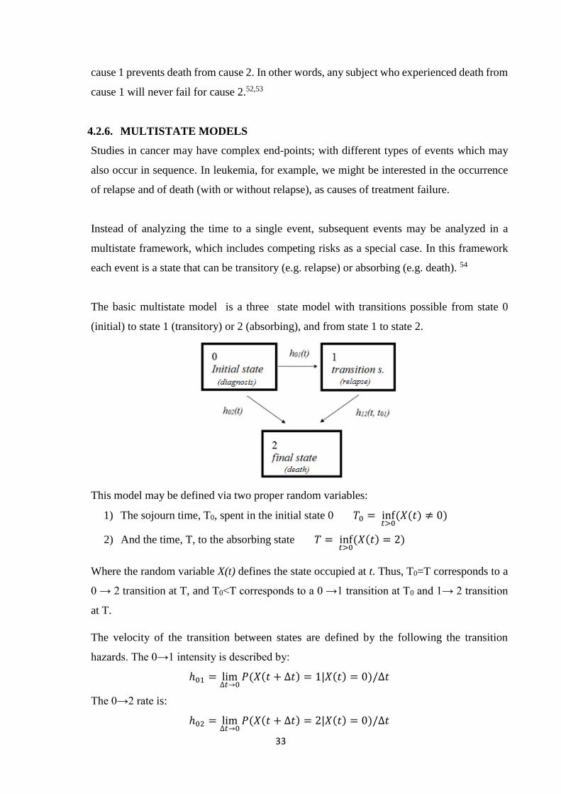
The basic multistate model is a three state model with transitions possible from state 0

(initial) to state 1 (transitory) or 2 (absorbing), and from state 1 to state 2.

This model may be defined via two proper random variables:

1) The sojourn time, T0, spent in the initial state 0 𝑇0 = inf𝑡>0

(𝑋(𝑡) ≠ 0)

2) And the time, T, to the absorbing state 𝑇 = inf𝑡>0

(𝑋(𝑡) = 2)

Where the random variable X(t) defines the state occupied at t. Thus, T0=T corresponds to a

0 → 2 transition at T, and T0<T corresponds to a 0 →1 transition at T0 and 1→ 2 transition

at T.

The velocity of the transition between states are defined by the following the transition

hazards. The 0→1 intensity is described by:

ℎ01 = lim∆𝑡→0

𝑃(𝑋(𝑡 + ∆𝑡) = 1|𝑋(𝑡) = 0)/∆𝑡

The 0→2 rate is:

ℎ02 = lim∆𝑡→0

𝑃(𝑋(𝑡 + ∆𝑡) = 2|𝑋(𝑡) = 0)/∆𝑡

34

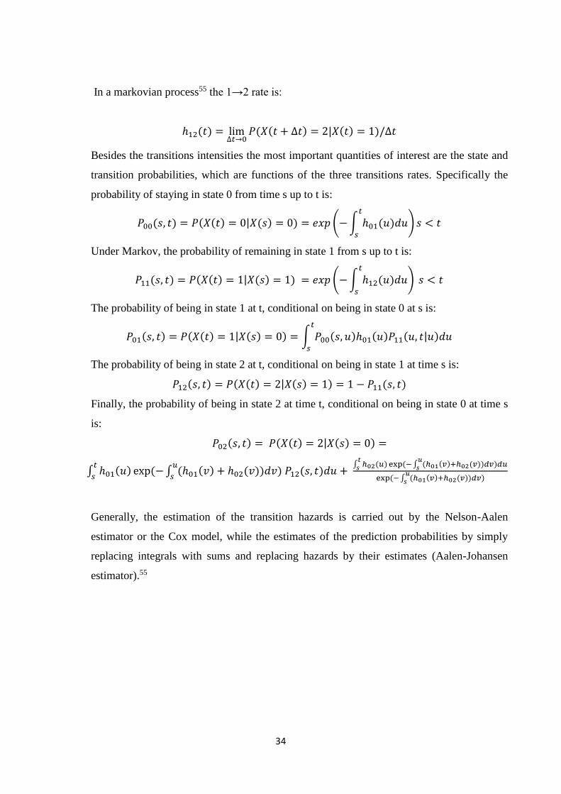
In a markovian process55 the 1→2 rate is:

ℎ12(𝑡) = lim∆𝑡→0

𝑃(𝑋(𝑡 + ∆𝑡) = 2|𝑋(𝑡) = 1)/∆𝑡

Besides the transitions intensities the most important quantities of interest are the state and

transition probabilities, which are functions of the three transitions rates. Specifically the

probability of staying in state 0 from time s up to t is:

𝑃00(𝑠, 𝑡) = 𝑃(𝑋(𝑡) = 0|𝑋(𝑠) = 0) = 𝑒𝑥𝑝 (− ∫ ℎ01(𝑢𝑡

𝑠

)𝑑𝑢) 𝑠 < 𝑡

Under Markov, the probability of remaining in state 1 from s up to t is:

𝑃11(𝑠, 𝑡) = 𝑃(𝑋(𝑡) = 1|𝑋(𝑠) = 1) = 𝑒𝑥𝑝 (− ∫ ℎ12(𝑢𝑡

𝑠

)𝑑𝑢) 𝑠 < 𝑡

The probability of being in state 1 at t, conditional on being in state 0 at s is:

𝑃01(𝑠, 𝑡) = 𝑃(𝑋(𝑡) = 1|𝑋(𝑠) = 0) = ∫ 𝑃00(𝑠, 𝑢)ℎ01(𝑢)𝑃11(𝑢, 𝑡|𝑢)𝑑𝑢𝑡

𝑠

The probability of being in state 2 at t, conditional on being in state 1 at time s is:

𝑃12(𝑠, 𝑡) = 𝑃(𝑋(𝑡) = 2|𝑋(𝑠) = 1) = 1 − 𝑃11(𝑠, 𝑡)

Finally, the probability of being in state 2 at time t, conditional on being in state 0 at time s

is:

𝑃02(𝑠, 𝑡) = 𝑃(𝑋(𝑡) = 2|𝑋(𝑠) = 0) =

∫ ℎ01(𝑢) exp(− ∫ (ℎ01(𝑣) + ℎ02(𝑣))𝑑𝑣) 𝑃12(𝑠, 𝑡)𝑑𝑢𝑢

𝑠

𝑡

𝑠+

∫ ℎ02(𝑢)𝑡

𝑠 exp(− ∫ (ℎ01(𝑣)+ℎ02(𝑣))𝑑𝑣)𝑑𝑢𝑢

𝑠

exp(− ∫ (ℎ01(𝑣)+ℎ02(𝑣))𝑑𝑣)𝑢

𝑠

Generally, the estimation of the transition hazards is carried out by the Nelson-Aalen

estimator or the Cox model, while the estimates of the prediction probabilities by simply

replacing integrals with sums and replacing hazards by their estimates (Aalen-Johansen

estimator).55

35

4.3. NON-STANDARD METHOD OF SURVIVAL ANALYSIS

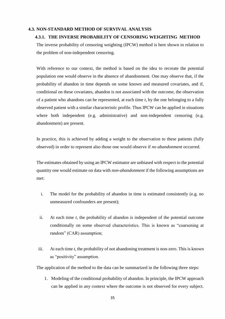
4.3.1. THE INVERSE PROBABILITY OF CENSORING WEIGHTING METHOD

The inverse probability of censoring weighting (IPCW) method is here shown in relation to

the problem of non-independent censoring.

With reference to our context, the method is based on the idea to recreate the potential

population one would observe in the absence of abandonment. One may observe that, if the

probability of abandon in time depends on some known and measured covariates, and if,

conditional on these covariates, abandon is not associated with the outcome, the observation

of a patient who abandons can be represented, at each time t, by the one belonging to a fully

observed patient with a similar characteristic profile. Thus IPCW can be applied in situations

where both independent (e.g. administrative) and non-independent censoring (e.g.

abandonment) are present.

In practice, this is achieved by adding a weight to the observation to these patients (fully

observed) in order to represent also those one would observe if no abandonment occurred.

The estimates obtained by using an IPCW estimator are unbiased with respect to the potential

quantity one would estimate on data with non-abandonment if the following assumptions are

met:

i. The model for the probability of abandon in time is estimated consistently (e.g. no

unmeasured confounders are present);

ii. At each time t, the probability of abandon is independent of the potential outcome

conditionally on some observed characteristics. This is known as “coarsening at

random” (CAR) assumption;

iii. At each time t, the probability of not abandoning treatment is non-zero. This is known

as “positivity” assumption.

The application of the method to the data can be summarized in the following three steps:

1. Modeling of the conditional probability of abandon. In principle, the IPCW approach

can be applied in any context where the outcome is not observed for every subject.

36

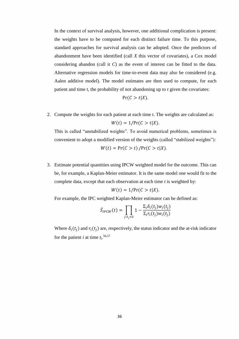
In the context of survival analysis, however, one additional complication is present:

the weights have to be computed for each distinct failure time. To this purpose,

standard approaches for survival analysis can be adopted. Once the predictors of

abandonment have been identified (call X this vector of covariates), a Cox model

considering abandon (call it C) as the event of interest can be fitted to the data.

Alternative regression models for time-to-event data may also be considered (e.g.

Aalen additive model). The model estimates are then used to compute, for each

patient and time t, the probability of not abandoning up to t given the covariates:

Pr (𝐶 > 𝑡|𝑋).

2. Compute the weights for each patient at each time t. The weights are calculated as:

𝑊(𝑡) = 1/Pr (𝐶 > 𝑡|𝑋).

This is called “unstabilized weights”. To avoid numerical problems, sometimes is

convenient to adopt a modified version of the weights (called “stabilized weights”):

𝑊(𝑡) = Pr(𝐶 > 𝑡) /Pr (𝐶 > 𝑡|𝑋).

3. Estimate potential quantities using IPCW weighted model for the outcome. This can

be, for example, a Kaplan-Meier estimator. It is the same model one would fit to the

complete data, except that each observation at each time t is weighted by:

𝑊(𝑡) = 1/Pr (𝐶 > 𝑡|𝑋).

For example, the IPC weighted Kaplan-Meier estimator can be defined as:

�̂�𝐼𝑃𝐶𝑊(𝑡) = ∏ 1 −Σ𝑖𝛿𝑖(𝑡𝑗)𝑤𝑖(𝑡𝑗)

Σ𝑖𝑟𝑖(𝑡𝑗)𝑤𝑖(𝑡𝑗)𝑗:𝑡𝑗<𝑡

Where 𝛿𝑖(𝑡𝑗) and 𝑟𝑖(𝑡𝑗) are, respectively, the status indicator and the at-risk indicator

for the patient i at time tj.56,57

37

5. RESULTS

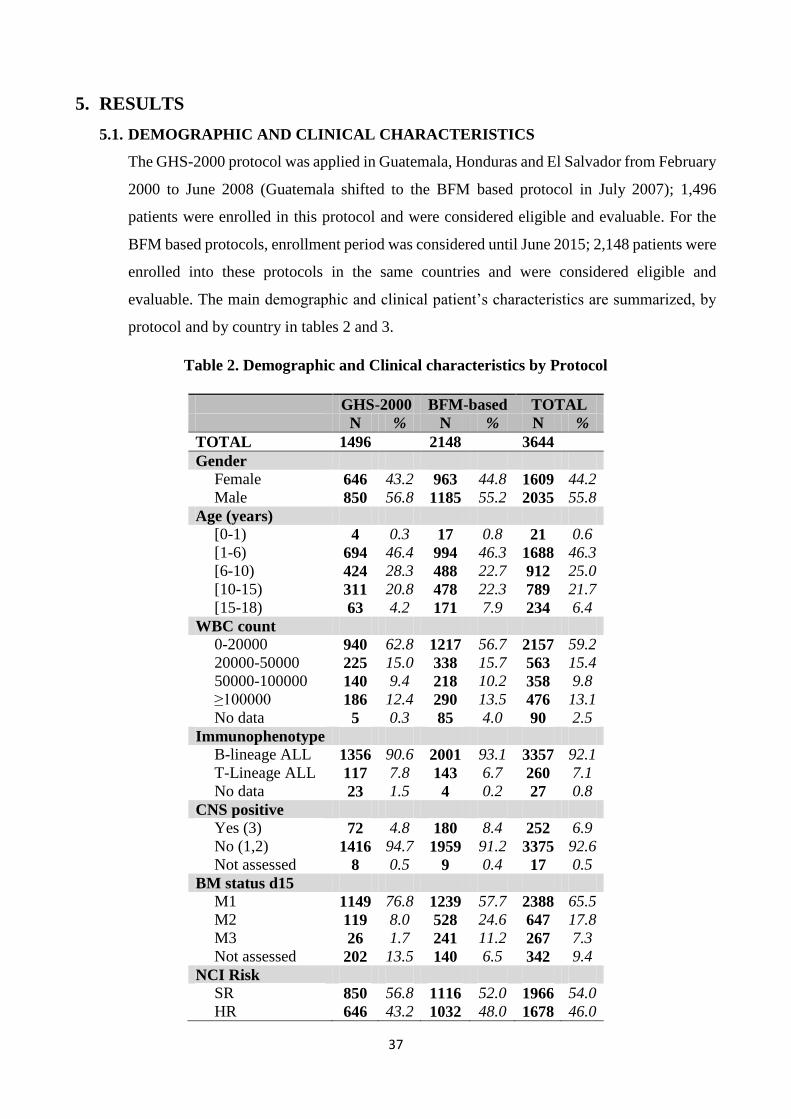
5.1. DEMOGRAPHIC AND CLINICAL CHARACTERISTICS

The GHS-2000 protocol was applied in Guatemala, Honduras and El Salvador from February

2000 to June 2008 (Guatemala shifted to the BFM based protocol in July 2007); 1,496

patients were enrolled in this protocol and were considered eligible and evaluable. For the

BFM based protocols, enrollment period was considered until June 2015; 2,148 patients were

enrolled into these protocols in the same countries and were considered eligible and

evaluable. The main demographic and clinical patient’s characteristics are summarized, by

protocol and by country in tables 2 and 3.

Table 2. Demographic and Clinical characteristics by Protocol

GHS-2000 BFM-based TOTAL N % N % N %

TOTAL 1496 2148 3644

Gender

Female 646 43.2 963 44.8 1609 44.2

Male 850 56.8 1185 55.2 2035 55.8

Age (years)

[0-1) 4 0.3 17 0.8 21 0.6

[1-6) 694 46.4 994 46.3 1688 46.3

[6-10) 424 28.3 488 22.7 912 25.0

[10-15) 311 20.8 478 22.3 789 21.7

[15-18) 63 4.2 171 7.9 234 6.4

WBC count

0-20000 940 62.8 1217 56.7 2157 59.2

20000-50000 225 15.0 338 15.7 563 15.4

50000-100000 140 9.4 218 10.2 358 9.8

≥100000 186 12.4 290 13.5 476 13.1

No data 5 0.3 85 4.0 90 2.5

Immunophenotype

B-lineage ALL 1356 90.6 2001 93.1 3357 92.1

T-Lineage ALL 117 7.8 143 6.7 260 7.1

No data 23 1.5 4 0.2 27 0.8

CNS positive

Yes (3) 72 4.8 180 8.4 252 6.9

No (1,2) 1416 94.7 1959 91.2 3375 92.6

Not assessed 8 0.5 9 0.4 17 0.5

BM status d15

M1 1149 76.8 1239 57.7 2388 65.5

M2 119 8.0 528 24.6 647 17.8

M3 26 1.7 241 11.2 267 7.3

Not assessed 202 13.5 140 6.5 342 9.4

NCI Risk

SR 850 56.8 1116 52.0 1966 54.0

HR 646 43.2 1032 48.0 1678 46.0

38

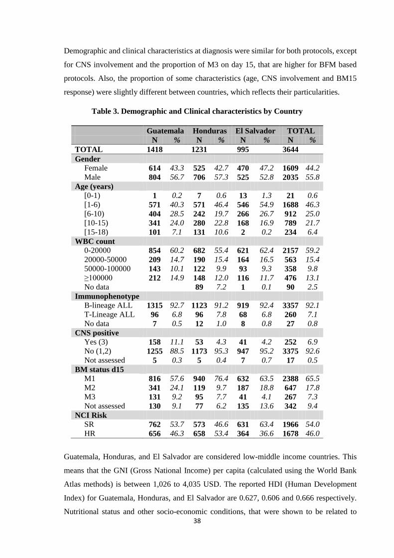
Demographic and clinical characteristics at diagnosis were similar for both protocols, except

for CNS involvement and the proportion of M3 on day 15, that are higher for BFM based

protocols. Also, the proportion of some characteristics (age, CNS involvement and BM15

response) were slightly different between countries, which reflects their particularities.

Table 3. Demographic and Clinical characteristics by Country

Guatemala Honduras El Salvador TOTAL N % N % N % N %

TOTAL 1418 1231 995 3644

Gender

Female 614 43.3 525 42.7 470 47.2 1609 44.2

Male 804 56.7 706 57.3 525 52.8 2035 55.8

Age (years)

[0-1) 1 0.2 7 0.6 13 1.3 21 0.6

[1-6) 571 40.3 571 46.4 546 54.9 1688 46.3

[6-10) 404 28.5 242 19.7 266 26.7 912 25.0

[10-15) 341 24.0 280 22.8 168 16.9 789 21.7

[15-18) 101 7.1 131 10.6 2 0.2 234 6.4

WBC count

0-20000 854 60.2 682 55.4 621 62.4 2157 59.2

20000-50000 209 14.7 190 15.4 164 16.5 563 15.4

50000-100000 143 10.1 122 9.9 93 9.3 358 9.8

≥100000 212 14.9 148 12.0 116 11.7 476 13.1

No data 89 7.2 1 0.1 90 2.5

Immunophenotype

B-lineage ALL 1315 92.7 1123 91.2 919 92.4 3357 92.1

T-Lineage ALL 96 6.8 96 7.8 68 6.8 260 7.1

No data 7 0.5 12 1.0 8 0.8 27 0.8

CNS positive

Yes (3) 158 11.1 53 4.3 41 4.2 252 6.9

No (1,2) 1255 88.5 1173 95.3 947 95.2 3375 92.6

Not assessed 5 0.3 5 0.4 7 0.7 17 0.5

BM status d15

M1 816 57.6 940 76.4 632 63.5 2388 65.5

M2 341 24.1 119 9.7 187 18.8 647 17.8

M3 131 9.2 95 7.7 41 4.1 267 7.3

Not assessed 130 9.1 77 6.2 135 13.6 342 9.4

NCI Risk

SR 762 53.7 573 46.6 631 63.4 1966 54.0

HR 656 46.3 658 53.4 364 36.6 1678 46.0

Guatemala, Honduras, and El Salvador are considered low-middle income countries. This

means that the GNI (Gross National Income) per capita (calculated using the World Bank

Atlas methods) is between 1,026 to 4,035 USD. The reported HDI (Human Development

Index) for Guatemala, Honduras, and El Salvador are 0.627, 0.606 and 0.666 respectively.

Nutritional status and other socio-economic conditions, that were shown to be related to

39

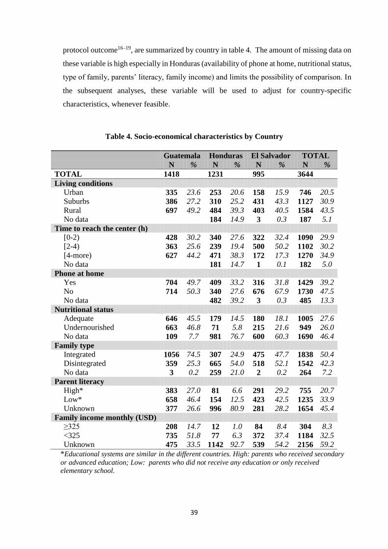
protocol outcome16–19, are summarized by country in table 4. The amount of missing data on

these variable is high especially in Honduras (availability of phone at home, nutritional status,

type of family, parents’ literacy, family income) and limits the possibility of comparison. In

the subsequent analyses, these variable will be used to adjust for country-specific

characteristics, whenever feasible.

Table 4. Socio-economical characteristics by Country

Guatemala Honduras El Salvador TOTAL N % N % N % N %

TOTAL 1418 1231 995 3644

Living conditions

Urban 335 23.6 253 20.6 158 15.9 746 20.5

Suburbs 386 27.2 310 25.2 431 43.3 1127 30.9

Rural 697 49.2 484 39.3 403 40.5 1584 43.5

No data 184 14.9 3 0.3 187 5.1

Time to reach the center (h)

[0-2) 428 30.2 340 27.6 322 32.4 1090 29.9

[2-4) 363 25.6 239 19.4 500 50.2 1102 30.2

[4-more) 627 44.2 471 38.3 172 17.3 1270 34.9

No data 181 14.7 1 0.1 182 5.0

Phone at home

Yes 704 49.7 409 33.2 316 31.8 1429 39.2

No 714 50.3 340 27.6 676 67.9 1730 47.5

No data 482 39.2 3 0.3 485 13.3

Nutritional status

Adequate 646 45.5 179 14.5 180 18.1 1005 27.6

Undernourished 663 46.8 71 5.8 215 21.6 949 26.0

No data 109 7.7 981 76.7 600 60.3 1690 46.4

Family type

Integrated 1056 74.5 307 24.9 475 47.7 1838 50.4

Disintegrated 359 25.3 665 54.0 518 52.1 1542 42.3

No data 3 0.2 259 21.0 2 0.2 264 7.2

Parent literacy

High* 383 27.0 81 6.6 291 29.2 755 20.7

Low* 658 46.4 154 12.5 423 42.5 1235 33.9

Unknown 377 26.6 996 80.9 281 28.2 1654 45.4

Family income monthly (USD)

≥325 208 14.7 12 1.0 84 8.4 304 8.3

<325 735 51.8 77 6.3 372 37.4 1184 32.5

Unknown 475 33.5 1142 92.7 539 54.2 2156 59.2

*Educational systems are similar in the different countries. High: parents who received secondary

or advanced education; Low: parents who did not receive any education or only received

elementary school.

40

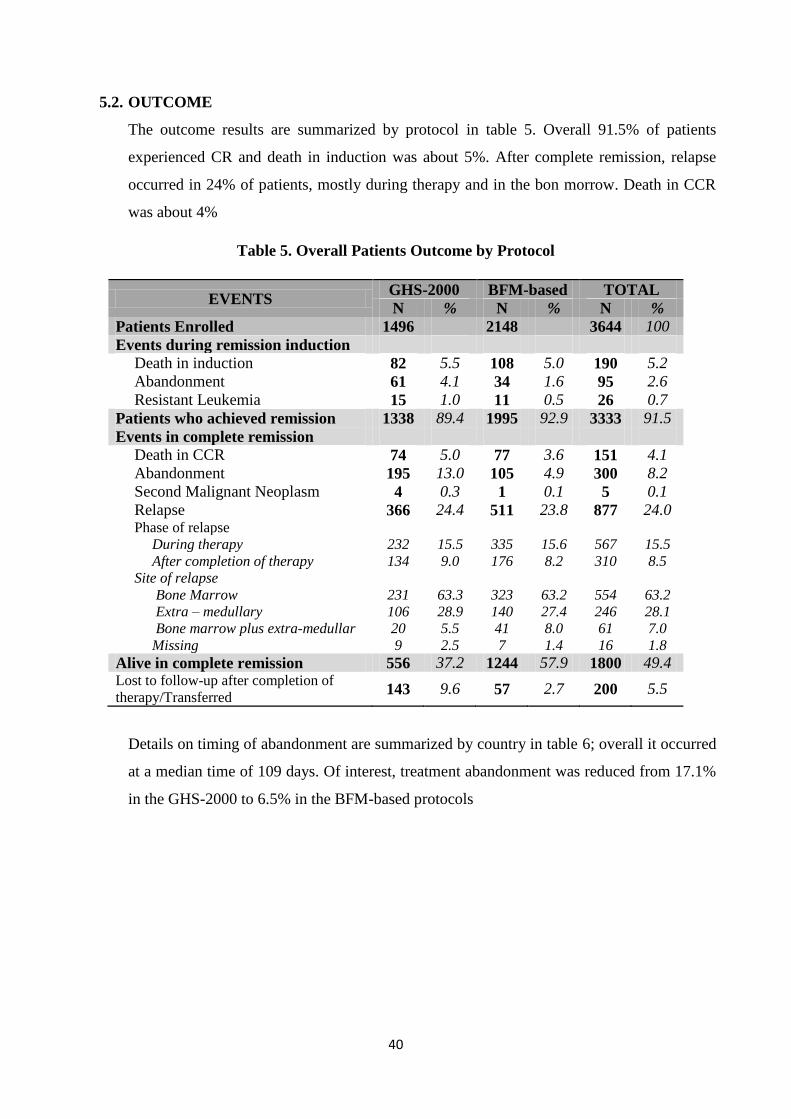
5.2. OUTCOME

The outcome results are summarized by protocol in table 5. Overall 91.5% of patients

experienced CR and death in induction was about 5%. After complete remission, relapse

occurred in 24% of patients, mostly during therapy and in the bon morrow. Death in CCR

was about 4%

Table 5. Overall Patients Outcome by Protocol

EVENTS GHS-2000 BFM-based TOTAL

N % N % N %

Patients Enrolled 1496 2148 3644 100

Events during remission induction

Death in induction 82 5.5 108 5.0 190 5.2

Abandonment 61 4.1 34 1.6 95 2.6

Resistant Leukemia 15 1.0 11 0.5 26 0.7

Patients who achieved remission 1338 89.4 1995 92.9 3333 91.5

Events in complete remission

Death in CCR 74 5.0 77 3.6 151 4.1

Abandonment 195 13.0 105 4.9 300 8.2

Second Malignant Neoplasm 4 0.3 1 0.1 5 0.1

Relapse 366 24.4 511 23.8 877 24.0 Phase of relapse

During therapy 232 15.5 335 15.6 567 15.5

After completion of therapy 134 9.0 176 8.2 310 8.5

Site of relapse

Bone Marrow 231 63.3 323 63.2 554 63.2

Extra – medullary 106 28.9 140 27.4 246 28.1

Bone marrow plus extra-medullar 20 5.5 41 8.0 61 7.0

Missing 9 2.5 7 1.4 16 1.8

Alive in complete remission 556 37.2 1244 57.9 1800 49.4 Lost to follow-up after completion of

therapy/Transferred 143 9.6 57 2.7 200 5.5

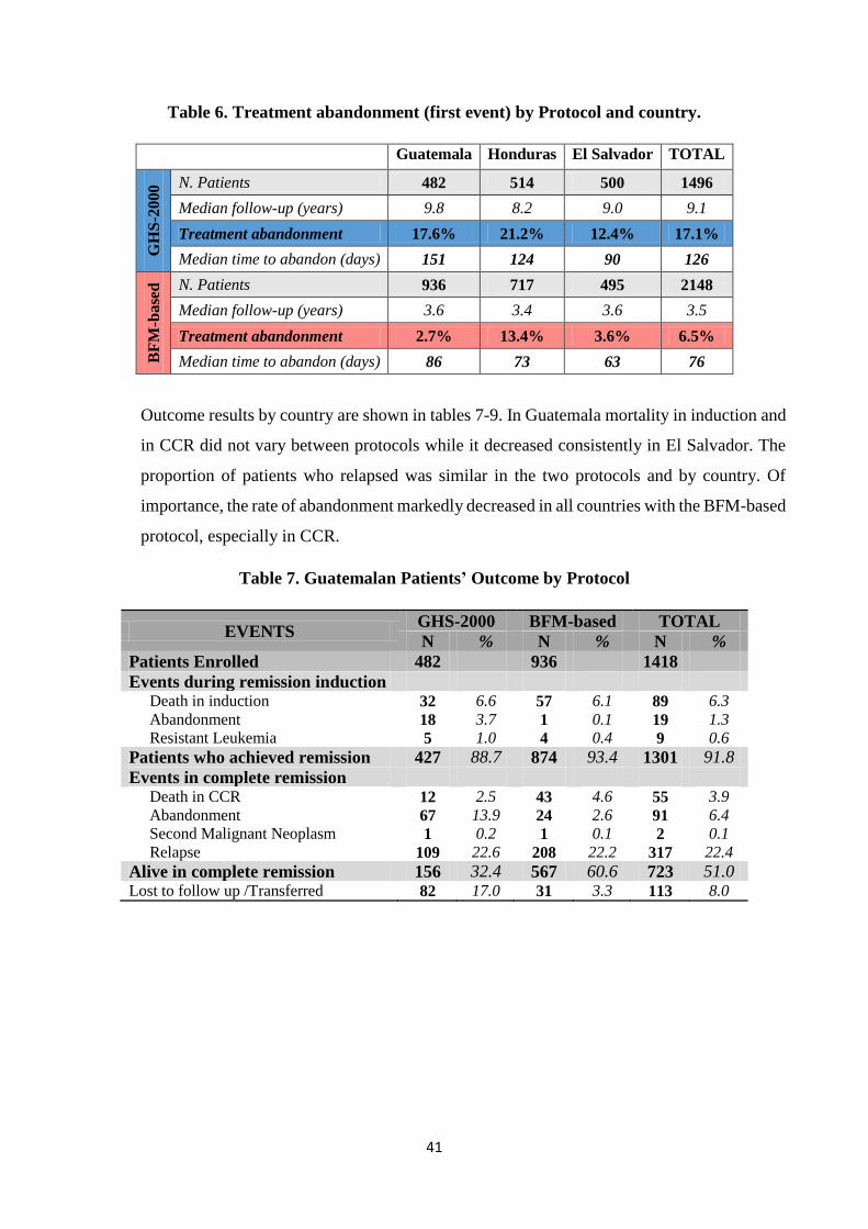
Details on timing of abandonment are summarized by country in table 6; overall it occurred

at a median time of 109 days. Of interest, treatment abandonment was reduced from 17.1%

in the GHS-2000 to 6.5% in the BFM-based protocols

41

Table 6. Treatment abandonment (first event) by Protocol and country.

Guatemala Honduras El Salvador TOTAL G

HS

-20

00 N. Patients 482 514 500 1496

Median follow-up (years) 9.8 8.2 9.0 9.1

Treatment abandonment 17.6% 21.2% 12.4% 17.1%

Median time to abandon (days) 151 124 90 126

BF

M-b

ase

d N. Patients 936 717 495 2148

Median follow-up (years) 3.6 3.4 3.6 3.5

Treatment abandonment 2.7% 13.4% 3.6% 6.5%

Median time to abandon (days) 86 73 63 76

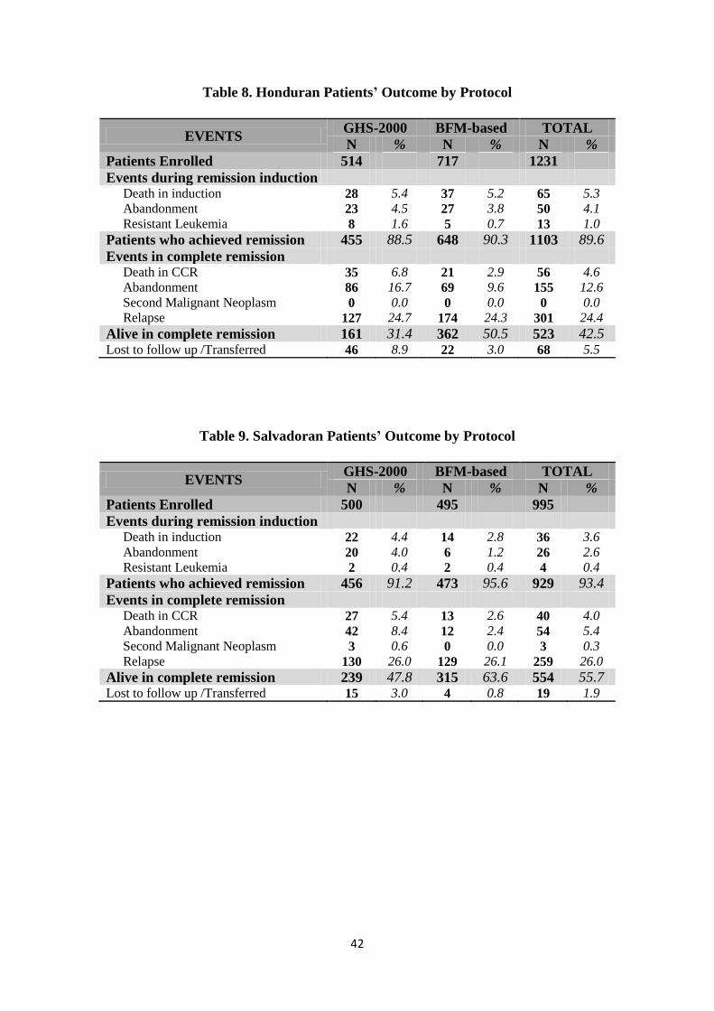
Outcome results by country are shown in tables 7-9. In Guatemala mortality in induction and

in CCR did not vary between protocols while it decreased consistently in El Salvador. The

proportion of patients who relapsed was similar in the two protocols and by country. Of

importance, the rate of abandonment markedly decreased in all countries with the BFM-based

protocol, especially in CCR.

Table 7. Guatemalan Patients’ Outcome by Protocol

EVENTS GHS-2000 BFM-based TOTAL

N % N % N %

Patients Enrolled 482 936 1418

Events during remission induction Death in induction 32 6.6 57 6.1 89 6.3

Abandonment 18 3.7 1 0.1 19 1.3

Resistant Leukemia 5 1.0 4 0.4 9 0.6

Patients who achieved remission 427 88.7 874 93.4 1301 91.8

Events in complete remission Death in CCR 12 2.5 43 4.6 55 3.9

Abandonment 67 13.9 24 2.6 91 6.4

Second Malignant Neoplasm 1 0.2 1 0.1 2 0.1

Relapse 109 22.6 208 22.2 317 22.4

Alive in complete remission 156 32.4 567 60.6 723 51.0 Lost to follow up /Transferred 82 17.0 31 3.3 113 8.0

42

Table 8. Honduran Patients’ Outcome by Protocol

EVENTS GHS-2000 BFM-based TOTAL

N % N % N %

Patients Enrolled 514 717 1231

Events during remission induction Death in induction 28 5.4 37 5.2 65 5.3

Abandonment 23 4.5 27 3.8 50 4.1

Resistant Leukemia 8 1.6 5 0.7 13 1.0

Patients who achieved remission 455 88.5 648 90.3 1103 89.6

Events in complete remission Death in CCR 35 6.8 21 2.9 56 4.6

Abandonment 86 16.7 69 9.6 155 12.6

Second Malignant Neoplasm 0 0.0 0 0.0 0 0.0

Relapse 127 24.7 174 24.3 301 24.4

Alive in complete remission 161 31.4 362 50.5 523 42.5 Lost to follow up /Transferred 46 8.9 22 3.0 68 5.5

Table 9. Salvadoran Patients’ Outcome by Protocol

EVENTS GHS-2000 BFM-based TOTAL

N % N % N %

Patients Enrolled 500 495 995

Events during remission induction Death in induction 22 4.4 14 2.8 36 3.6

Abandonment 20 4.0 6 1.2 26 2.6

Resistant Leukemia 2 0.4 2 0.4 4 0.4

Patients who achieved remission 456 91.2 473 95.6 929 93.4

Events in complete remission Death in CCR 27 5.4 13 2.6 40 4.0

Abandonment 42 8.4 12 2.4 54 5.4

Second Malignant Neoplasm 3 0.6 0 0.0 3 0.3

Relapse 130 26.0 129 26.1 259 26.0

Alive in complete remission 239 47.8 315 63.6 554 55.7 Lost to follow up /Transferred 15 3.0 4 0.8 19 1.9

43

5.3. SURVIVAL ANALYSIS WITH THE STANDARD APPROACH

5.3.1. ABANDONMENT AS EVENT

The following analysis considers abandonment as failure of the approach to cure and as such

abandonment is counted as an event. By contrast curves are estimated also considering

abandonment as non informative censored observation.

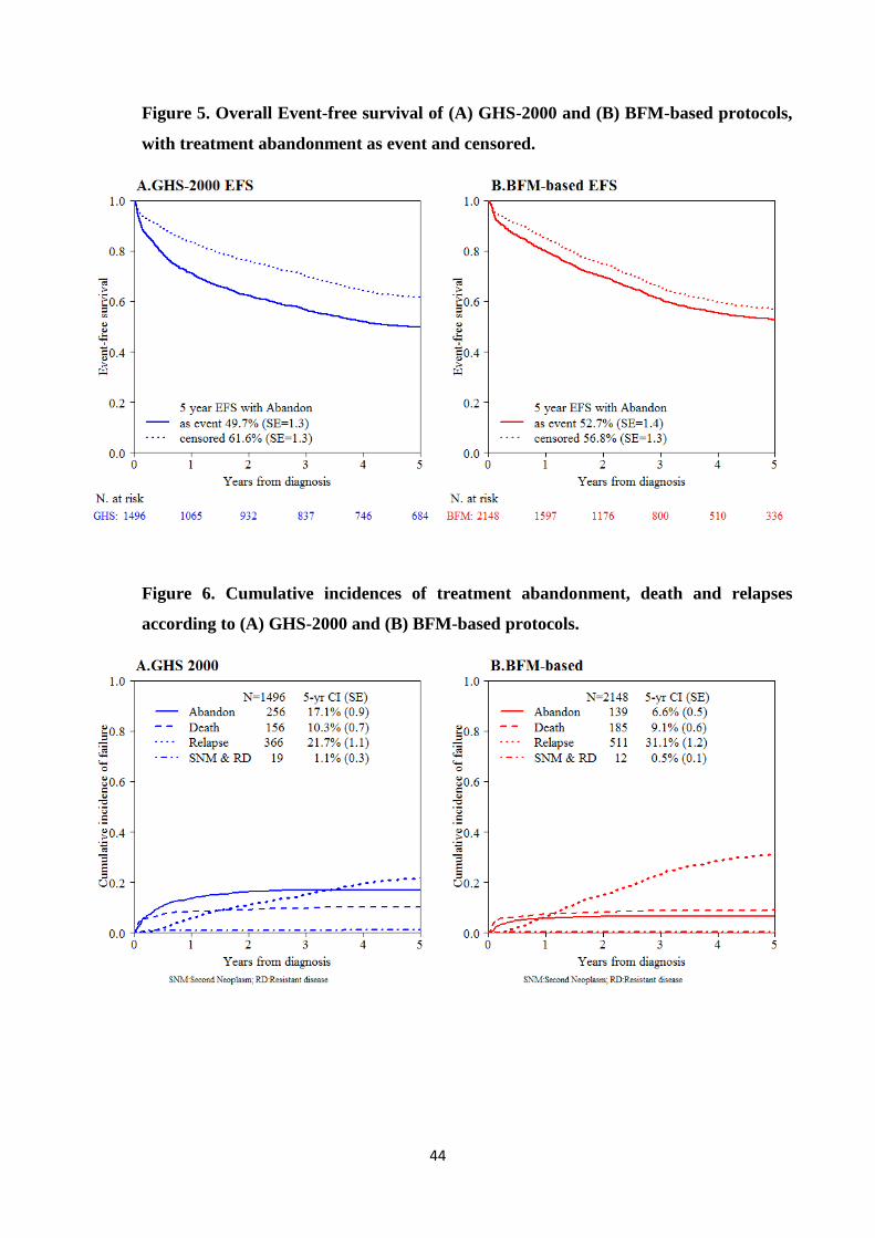
For GHS-2000 protocol, with a median observation time of 9.1 years, considering

abandonment as an event, the 5-year event-free and overall survival estimates obtained by

the Kaplan-Meier method were 49.7% (SE = 1.3%) and 55.8% (SE = 1.3%), respectively,

while censoring abandonment, the 5-year EFS and overall survival were 61.6% (SE = 1.3%)

and 64.7% (SE = 1.3%), respectively. The 5-year cumulative incidence (CI) rates for death,

relapse and treatment abandonment, estimated by Aalen-Johansen method, were 10.3% (SE

= 0.6%), 22.8% (SE = 1.1%) and 17.1% (SE = 0.9%) respectively. (Figure 5A and 6A)

In the BFM-based protocols, with a median observation time of 3.8 years, when abandonment

was considered an event, the 5-year event-free and overall survival estimates were 52.7%

(SE = 1.3%) and 62.3% (SE = 1.3%), respectively, while censoring abandonment, the 5-year

EFS and overall survival were 56.8% (SE = 1.4%) and 65.7% (SE = 1.3%), respectively. The

5-year CI rates for death, relapse and treatment abandonment were 9.1% (SE = 0.4%), 31.6%

(SE = 1.5%) and 6.6% (SE=0.9%) respectively. (Figure 5B and 6B)

44

Figure 5. Overall Event-free survival of (A) GHS-2000 and (B) BFM-based protocols,

with treatment abandonment as event and censored.

Figure 6. Cumulative incidences of treatment abandonment, death and relapses

according to (A) GHS-2000 and (B) BFM-based protocols.

45

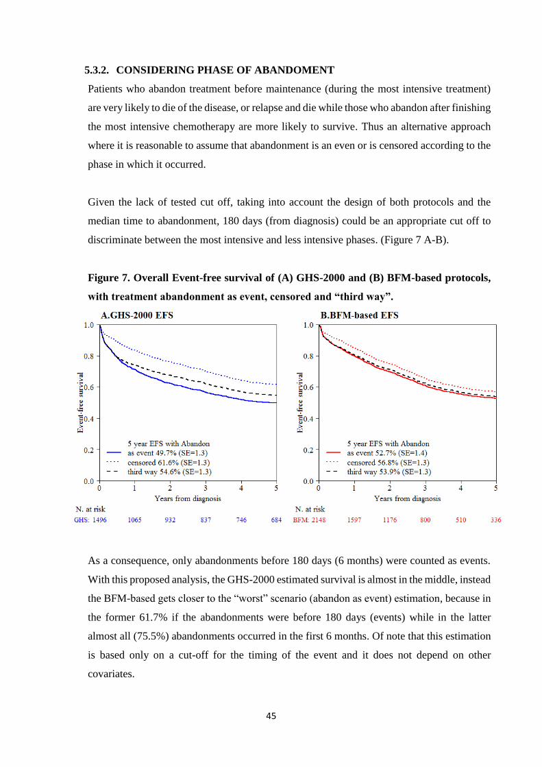
5.3.2. CONSIDERING PHASE OF ABANDOMENT

Patients who abandon treatment before maintenance (during the most intensive treatment)

are very likely to die of the disease, or relapse and die while those who abandon after finishing

the most intensive chemotherapy are more likely to survive. Thus an alternative approach

where it is reasonable to assume that abandonment is an even or is censored according to the

phase in which it occurred.

Given the lack of tested cut off, taking into account the design of both protocols and the

median time to abandonment, 180 days (from diagnosis) could be an appropriate cut off to

discriminate between the most intensive and less intensive phases. (Figure 7 A-B).

Figure 7. Overall Event-free survival of (A) GHS-2000 and (B) BFM-based protocols,

with treatment abandonment as event, censored and “third way”.

As a consequence, only abandonments before 180 days (6 months) were counted as events.

With this proposed analysis, the GHS-2000 estimated survival is almost in the middle, instead

the BFM-based gets closer to the “worst” scenario (abandon as event) estimation, because in

the former 61.7% if the abandonments were before 180 days (events) while in the latter

almost all (75.5%) abandonments occurred in the first 6 months. Of note that this estimation

is based only on a cut-off for the timing of the event and it does not depend on other

covariates.

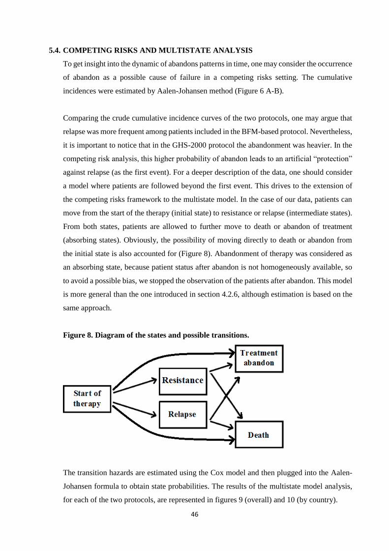
46

5.4. COMPETING RISKS AND MULTISTATE ANALYSIS

To get insight into the dynamic of abandons patterns in time, one may consider the occurrence

of abandon as a possible cause of failure in a competing risks setting. The cumulative

incidences were estimated by Aalen-Johansen method (Figure 6 A-B).

Comparing the crude cumulative incidence curves of the two protocols, one may argue that

relapse was more frequent among patients included in the BFM-based protocol. Nevertheless,

it is important to notice that in the GHS-2000 protocol the abandonment was heavier. In the

competing risk analysis, this higher probability of abandon leads to an artificial “protection”

against relapse (as the first event). For a deeper description of the data, one should consider

a model where patients are followed beyond the first event. This drives to the extension of

the competing risks framework to the multistate model. In the case of our data, patients can

move from the start of the therapy (initial state) to resistance or relapse (intermediate states).

From both states, patients are allowed to further move to death or abandon of treatment

(absorbing states). Obviously, the possibility of moving directly to death or abandon from

the initial state is also accounted for (Figure 8). Abandonment of therapy was considered as

an absorbing state, because patient status after abandon is not homogeneously available, so

to avoid a possible bias, we stopped the observation of the patients after abandon. This model

is more general than the one introduced in section 4.2.6, although estimation is based on the

same approach.

Figure 8. Diagram of the states and possible transitions.

The transition hazards are estimated using the Cox model and then plugged into the Aalen-

Johansen formula to obtain state probabilities. The results of the multistate model analysis,

for each of the two protocols, are represented in figures 9 (overall) and 10 (by country).

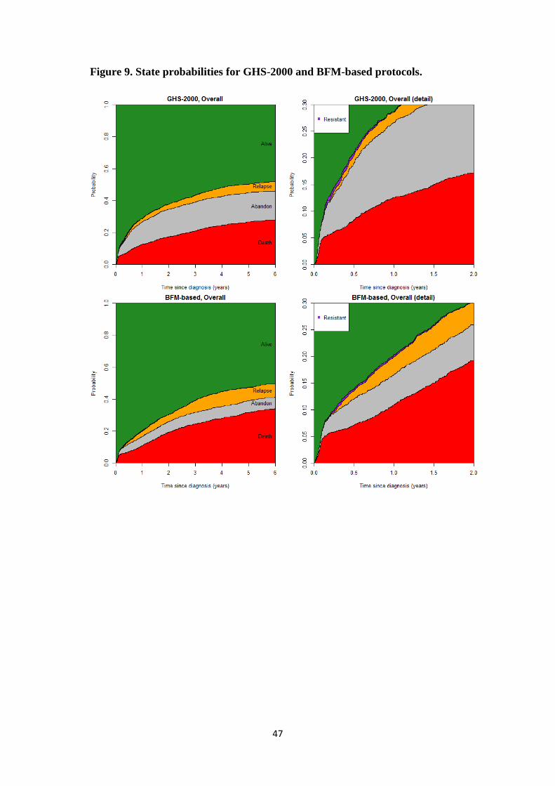
47

Figure 9. State probabilities for GHS-2000 and BFM-based protocols.

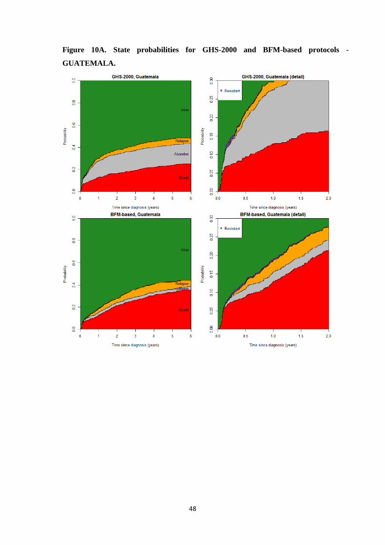
48

Figure 10A. State probabilities for GHS-2000 and BFM-based protocols -

GUATEMALA.

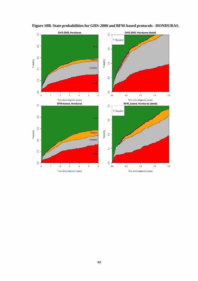
49

Figure 10B. State probabilities for GHS-2000 and BFM-based protocols - HONDURAS.

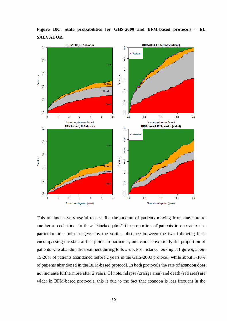
50

Figure 10C. State probabilities for GHS-2000 and BFM-based protocols – EL

SALVADOR.

This method is very useful to describe the amount of patients moving from one state to

another at each time. In these “stacked plots” the proportion of patients in one state at a

particular time point is given by the vertical distance between the two following lines

encompassing the state at that point. In particular, one can see explicitly the proportion of

patients who abandon the treatment during follow-up. For instance looking at figure 9, about

15-20% of patients abandoned before 2 years in the GHS-2000 protocol, while about 5-10%

of patients abandoned in the BFM-based protocol. In both protocols the rate of abandon does

not increase furthermore after 2 years. Of note, relapse (orange area) and death (red area) are

wider in BFM-based protocols, this is due to the fact that abandon is less frequent in the

51

recent protocols. From pictures 10 A, B, C it is also evident that the most recent protocol has

a lower rate of abandon in all countries.

The plots on the right-hand side represent a detail of the left-hand side figures (the time scale

is 2 years instead of 6 years and the vertical axis does not go to 1) to visualize the amount of

patients developing a treatment resistance. The multistate analysis provides a clear picture of

the observed outcomes in time. However, it does not allow to “remove” the effect of

abandonment from survival. In order to focus on the potential outcomes we would observe

under no abandonment, the IPCW method was applied.

5.5. RESULTS OF IPCW METHOD

As mentioned in section 4.3.1 a crucial assumption for the validity of the IPCW method is

that the probability of abandon for a patient with a given prognosis depends only on the

covariates included in the model for predicting abandon. Thus, these covariates must be

related to both the outcome and to the propensity to abandon treatment.

First of all, we considered the following clinical and biological features: gender, age, WBC

count at diagnosis, ALL-linage, CNS involvement, BM status on day 15 (was the common

measure response for both protocols). These covariates are usually used as risk stratification

criteria, because they identifies subgroups of patients at different prognosis.

In addition, the available information on socio-economic factors such as living conditions,

time to arrive to the treatment center, the availability of phone at home, the type of family

(this somehow represent a support system for the patient and its caregiver) and parental

literacy was considered. We selected these factors based on the findings published in the

literature on this topic. 16–19

It was observed that the risk of abandonment was associated with different factors in each

country, we decided to perform three different analyses, one for each country. Indeed, to

perform a single overall analysis one would have included an interaction term between the

country indicator and each other factor, increasing the complexity and possibly reducing the

precision of the estimates.

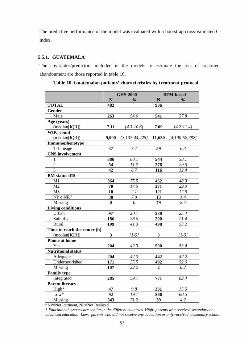
52

The predictive performance of the model was evaluated with a bootstrap cross-validated C-

index.

5.5.1. GUATEMALA

The covariates/predictors included in the models to estimate the risk of treatment

abandonment are those reported in table 10.

Table 10. Guatemalan patients’ characteristics by treatment protocol

GHS-2000 BFM-based

N % N %

TOTAL 482 936

Gender

Male 263 54.6 541 57.8

Age (years)

(median[IQR]) 7.11 [4.3-10.6] 7.09 [4.2-11.4]

WBC count

(median[IQR]) 9,000 [3,137-44,425] 11,630 [4,190-52,782]

Immunophenotype

T-Lineage 37 7.7 59 6.3

CNS involvement

1 386 80.1 544 58.1

2 54 11.2 276 29.5

3 42 8.7 116 12.4

BM status d15

M1 364 75.5 452 48.3

M2 70 14.5 271 29.0

M3 10 2.1 121 12.9

NP o NR a 38 7.9 13 1.4

Missing 0 0 79 8.4

Living conditions

Urban 97 20.1 238 25.4

Suburbs 186 38.6 200 21.4

Rural 199 41.3 498 53.2

Time to reach the center (h)

(median[IQR]) 3 [1-5] 3 [1-5]

Phone at home

Yes 204 42.3 500 53.4

Nutritional status

Adequate 204 42.3 442 47.2

Undernourished 171 35.5 492 52.6

Missing 107 22.2 2 0.2

Family type

Integrated 285 59.1 771 82.4

Parent literacy

High* 47 9.8 331 35.5

Low* 92 19.1 566 60.5

Missing 343 71.2 39 4.2 a NP=Not Pertinent, NR=Not Realized.

* Educational systems are similar in the different countries. High: parents who received secondary or

advanced education; Low: parents who did not receive any education or only received elementary school.

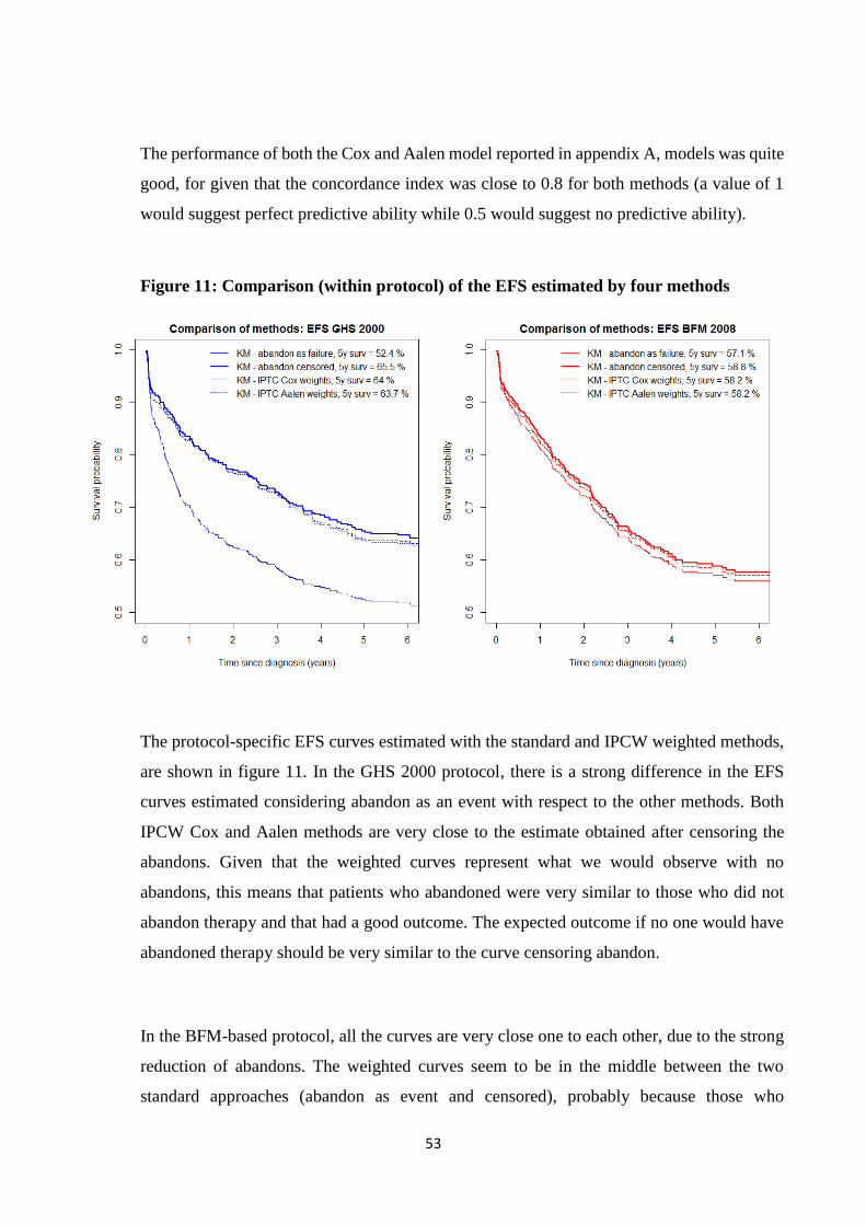
53

The performance of both the Cox and Aalen model reported in appendix A, models was quite

good, for given that the concordance index was close to 0.8 for both methods (a value of 1

would suggest perfect predictive ability while 0.5 would suggest no predictive ability).

Figure 11: Comparison (within protocol) of the EFS estimated by four methods

The protocol-specific EFS curves estimated with the standard and IPCW weighted methods,

are shown in figure 11. In the GHS 2000 protocol, there is a strong difference in the EFS

curves estimated considering abandon as an event with respect to the other methods. Both

IPCW Cox and Aalen methods are very close to the estimate obtained after censoring the

abandons. Given that the weighted curves represent what we would observe with no

abandons, this means that patients who abandoned were very similar to those who did not

abandon therapy and that had a good outcome. The expected outcome if no one would have

abandoned therapy should be very similar to the curve censoring abandon.

In the BFM-based protocol, all the curves are very close one to each other, due to the strong

reduction of abandons. The weighted curves seem to be in the middle between the two

standard approaches (abandon as event and censored), probably because those who

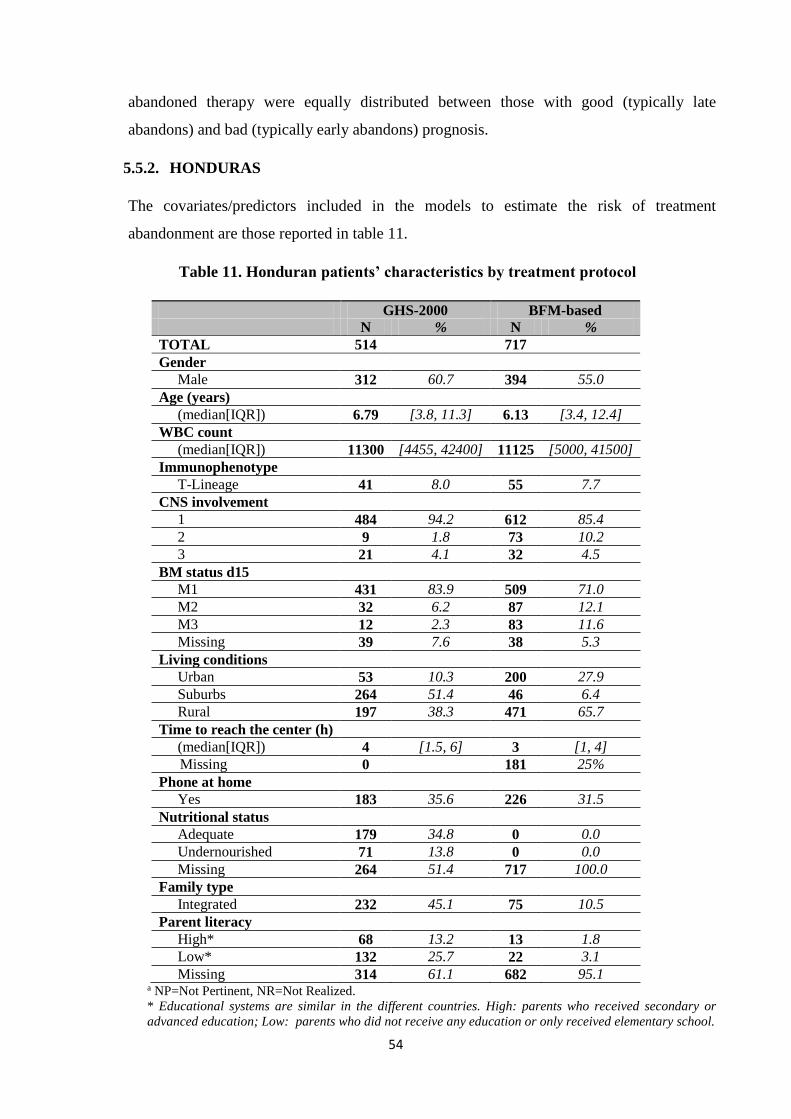
54

abandoned therapy were equally distributed between those with good (typically late

abandons) and bad (typically early abandons) prognosis.

5.5.2. HONDURAS

The covariates/predictors included in the models to estimate the risk of treatment

abandonment are those reported in table 11.

Table 11. Honduran patients’ characteristics by treatment protocol

GHS-2000 BFM-based

N % N %

TOTAL 514 717

Gender

Male 312 60.7 394 55.0

Age (years)

(median[IQR]) 6.79 [3.8, 11.3] 6.13 [3.4, 12.4]

WBC count

(median[IQR]) 11300 [4455, 42400] 11125 [5000, 41500]

Immunophenotype

T-Lineage 41 8.0 55 7.7

CNS involvement

1 484 94.2 612 85.4

2 9 1.8 73 10.2

3 21 4.1 32 4.5

BM status d15

M1 431 83.9 509 71.0

M2 32 6.2 87 12.1

M3 12 2.3 83 11.6

Missing 39 7.6 38 5.3

Living conditions

Urban 53 10.3 200 27.9

Suburbs 264 51.4 46 6.4

Rural 197 38.3 471 65.7

Time to reach the center (h)

(median[IQR]) 4 [1.5, 6] 3 [1, 4]

Missing 0 181 25%

Phone at home

Yes 183 35.6 226 31.5

Nutritional status

Adequate 179 34.8 0 0.0

Undernourished 71 13.8 0 0.0

Missing 264 51.4 717 100.0

Family type

Integrated 232 45.1 75 10.5

Parent literacy

High* 68 13.2 13 1.8

Low* 132 25.7 22 3.1

Missing 314 61.1 682 95.1 a NP=Not Pertinent, NR=Not Realized.

* Educational systems are similar in the different countries. High: parents who received secondary or

advanced education; Low: parents who did not receive any education or only received elementary school.

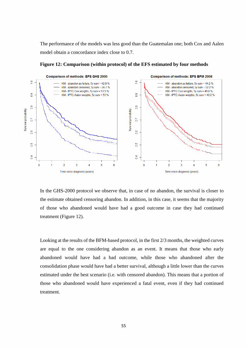
55

The performance of the models was less good than the Guatemalan one; both Cox and Aalen

model obtain a concordance index close to 0.7.

Figure 12: Comparison (within protocol) of the EFS estimated by four methods

In the GHS-2000 protocol we observe that, in case of no abandon, the survival is closer to

the estimate obtained censoring abandon. In addition, in this case, it seems that the majority

of those who abandoned would have had a good outcome in case they had continued

treatment (Figure 12).

Looking at the results of the BFM-based protocol, in the first 2/3 months, the weighted curves

are equal to the one considering abandon as an event. It means that those who early

abandoned would have had a bad outcome, while those who abandoned after the

consolidation phase would have had a better survival, although a little lower than the curves

estimated under the best scenario (i.e. with censored abandon). This means that a portion of

those who abandoned would have experienced a fatal event, even if they had continued

treatment.

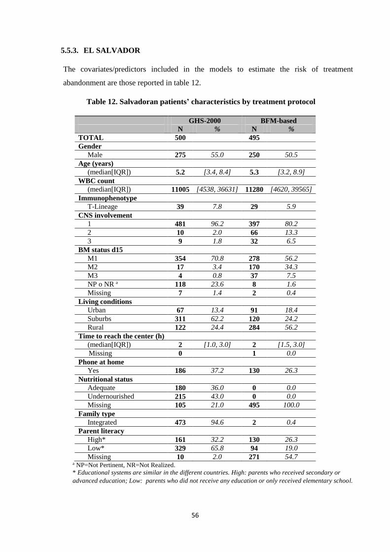
56

5.5.3. EL SALVADOR

The covariates/predictors included in the models to estimate the risk of treatment

abandonment are those reported in table 12.

Table 12. Salvadoran patients’ characteristics by treatment protocol

GHS-2000 BFM-based

N % N %

TOTAL 500 495

Gender

Male 275 55.0 250 50.5

Age (years)

(median[IQR]) 5.2 [3.4, 8.4] 5.3 [3.2, 8.9]

WBC count

(median[IQR]) 11005 [4538, 36631] 11280 [4620, 39565]

Immunophenotype

T-Lineage 39 7.8 29 5.9

CNS involvement

1 481 96.2 397 80.2

2 10 2.0 66 13.3

3 9 1.8 32 6.5

BM status d15

M1 354 70.8 278 56.2

M2 17 3.4 170 34.3

M3 4 0.8 37 7.5

NP o NR a 118 23.6 8 1.6

Missing 7 1.4 2 0.4

Living conditions

Urban 67 13.4 91 18.4

Suburbs 311 62.2 120 24.2

Rural 122 24.4 284 56.2

Time to reach the center (h)

(median[IQR]) 2 [1.0, 3.0] 2 [1.5, 3.0]

Missing 0 1 0.0

Phone at home

Yes 186 37.2 130 26.3

Nutritional status

Adequate 180 36.0 0 0.0

Undernourished 215 43.0 0 0.0

Missing 105 21.0 495 100.0

Family type

Integrated 473 94.6 2 0.4

Parent literacy

High* 161 32.2 130 26.3

Low* 329 65.8 94 19.0

Missing 10 2.0 271 54.7 a NP=Not Pertinent, NR=Not Realized.

* Educational systems are similar in the different countries. High: parents who received secondary or

advanced education; Low: parents who did not receive any education or only received elementary school.

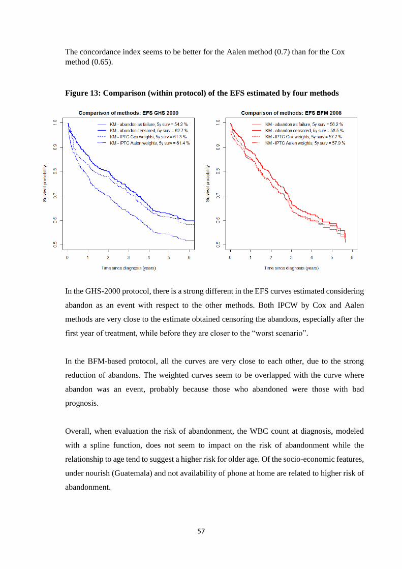
57

The concordance index seems to be better for the Aalen method (0.7) than for the Cox

method (0.65).

Figure 13: Comparison (within protocol) of the EFS estimated by four methods

In the GHS-2000 protocol, there is a strong different in the EFS curves estimated considering

abandon as an event with respect to the other methods. Both IPCW by Cox and Aalen

methods are very close to the estimate obtained censoring the abandons, especially after the

first year of treatment, while before they are closer to the “worst scenario”.

In the BFM-based protocol, all the curves are very close to each other, due to the strong

reduction of abandons. The weighted curves seem to be overlapped with the curve where

abandon was an event, probably because those who abandoned were those with bad

prognosis.

Overall, when evaluation the risk of abandonment, the WBC count at diagnosis, modeled

with a spline function, does not seem to impact on the risk of abandonment while the

relationship to age tend to suggest a higher risk for older age. Of the socio-economic features,

under nourish (Guatemala) and not availability of phone at home are related to higher risk of

abandonment.

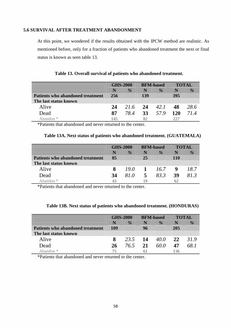
58

5.6 SURVIVAL AFTER TREATMENT ABANDONMENT

At this point, we wondered if the results obtained with the IPCW method are realistic. As

mentioned before, only for a fraction of patients who abandoned treatment the next or final

status is known as seen table 13.

Table 13. Overall survival of patients who abandoned treatment.

GHS-2000 BFM-based TOTAL

N % N % N %

Patients who abandoned treatment 256 139 395

The last status known

Alive 24 21.6 24 42.1 48 28.6

Dead 87 78.4 33 57.9 120 71.4 Abandon * 145 82 227

*Patients that abandoned and never returned to the center.

Table 13A. Next status of patients who abandoned treatment. (GUATEMALA)

GHS-2000 BFM-based TOTAL

N % N % N %

Patients who abandoned treatment 85 25 110

The last status known

Alive 8 19.0 1 16.7 9 18.7

Dead 34 81.0 5 83.3 39 81.3 Abandon * 43 19 62

*Patients that abandoned and never returned to the center.

Table 13B. Next status of patients who abandoned treatment. (HONDURAS)

GHS-2000 BFM-based TOTAL

N % N % N %

Patients who abandoned treatment 109 96 205

The last status known

Alive 8 23.5 14 40.0 22 31.9

Dead 26 76.5 21 60.0 47 68.1 Abandon * 75 61 136

*Patients that abandoned and never returned to the center.

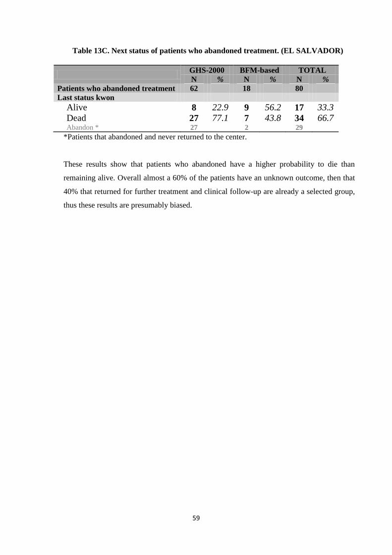
59

Table 13C. Next status of patients who abandoned treatment. (EL SALVADOR)

GHS-2000 BFM-based TOTAL

N % N % N %

Patients who abandoned treatment 62 18 80

Last status kwon

Alive 8 22.9 9 56.2 17 33.3

Dead 27 77.1 7 43.8 34 66.7 Abandon * 27 2 29

*Patients that abandoned and never returned to the center.

These results show that patients who abandoned have a higher probability to die than

remaining alive. Overall almost a 60% of the patients have an unknown outcome, then that

40% that returned for further treatment and clinical follow-up are already a selected group,

thus these results are presumably biased.

60

6. DISCUSSION

A key characteristic of the collected survival data in the framework of the AHOPCA network is

the presence of dropouts during treatment (treatment abandonment). In the past, treatment

abandon reached 50% in some countries of AHOPCA like Nicaragua or Honduras1. Table 6

showed that in the last two decades in these three countries abandonment reached 17.1% of

children under front line treatment for ALL protocols.

Children with ALL who abandon therapy are indeed likely to die for disease progression,

especially when they abandon in an early phase of treatment and clinical centers are rarely able

to retrace them and to update the information on their status. For this reason and for the fact that

abandonment is, per se, a failure in treatment policy, abandon is considered an event in the

estimation of survival or event free survival probability. This type of analysis is referred as “worst

scenario” evaluation since abandonment is included in the definition of the survival time as cause

of failure. Sometimes some selected cases come back to the hospital after dropout to seek for

more care, thus it was proposed to censored abandonment, since in principle there is no certainty

of death after treatment abandonment, especially if it occurs in the last phase of treatment

(maintenance) and this type of analysis is referred as “best scenario” evaluation which gives a

higher survival probability than the former scenario.

Of note, the “best scenario” approach assumes non-informative censoring due to abandonment,

which cannot be formally validated. This assumption is obviously unrealistic and, is not even

appropriate for describing the protocol outcome as it is likely to be biased. Abandonment (like

noncompliance), is often related to the clinical condition of a patient, either very bad, such as to

discourage the family in continuing treatment (typical of early dropouts) or quite good, such as to

provide the illusion that therapy can be safely omitted (typical of late drop-outs).

The “worst” scenario does not require the assumption of non informative censoring and is also

useful from a public health perspective since it considers abandonment as a failure of the clinical

center and of the health system. However, these analyses cannot provide insights into the potential

outcome in absence of abandonment. We can only consider that the “truth” on the clinical

outcome of the front line treatment in the presence of abandonment is likely to lie between the

two estimated curves (worst and best scenario).15

61

Another approach could be to estimate the outcome treating abandonment as event (failure) or

censored observation according to the phase of treatment when it occurred: a failure for patients

who abandoned treatment before starting maintenance and censored observation for those who

abandoned treatment during maintenance phase. This approach makes a “deterministic” choice

on how to handle drop-out and, although interesting to consider when no data are available on the

type of patients who abandoned, is quite arbitrary (Figure 7).

The issue on how to handle informative censoring thus needs to be addressed with other statistical

methods that take into account the covariates that characterize those patients who abandon with

the aim to obtain a more accurate estimate of probability of survival. In particular, in our case

example, treatment abandonment is not necessarily related to the disease or the treatment side

effects, as we are used to assume in clinical trials conducted in Italy or richer countries. In the

setting of low-income countries, poor socio-economic conditions, distance from the specialized

treatment center, parental illiteracy, living conditions and cultural background are important

factors shown to be related with a higher risk of treatment abandonment 16–18. From a clinical

perspective, however, the question of clinical interest is on the impact of the treatment protocol

per se and the question is: what would the unobserved event-free survival be in case no one would

have abandoned the treatment? The challenge posed by this question seems to be more evident

when the rate of abandonment exceeds 5-10% level (as in our case of study).

In summary, we cannot assume that all patients that abandon will die (even when in some cases

this could be realistic) neither that all patients that abandon will be alive free from disease

progression, because both assumptions are unrealistic. The outcome estimates obtained with the

current approaches (Figure 5, “best” and “worst” scenario) can be considered as the boundaries

of the true outcome, and it is necessary to look for new methodologies to estimate the outcome as

if no abandon occurred.

The competing risks approach could help in describing the impact of treatment abandonment on

survival adjusting for the competing effect of the other events. Multistate models extend this

framework allowing some states to be transitory (e.g. resistance, relapse). The multistate analysis

is helpful to describe the proportion of patients in each state during time, as it become clear in the

panels of figure 10. However, it does not allow to “remove” the effect of abandonment from

survival and to answer the clinical question on treatment effect.

62

In order to focus on the potential outcomes we would observe under no abandonment, we propose

to apply an IPCW approach to estimation. This approach estimates survival probabilities after

weighting fully observed patients in order to artificially represent the censored outcome of

patients with similar characteristics who abandoned. In this approach the observation of a patient

who abandons can be represented, at each time t, by one belonging to a fully observed patient

with similar characteristic profile.

To apply this method we assume that that the probability of abandon for a patient with a given

prognosis depends only on the covariates included in the model for predicting abandonment.

Thus, these covariates, such as clinical and biological features, and socio-economic factors must

be related to both the outcome and to the propensity to abandon treatment (see appendices A1,

B1 and C1). However other crucial factors that can help in predicting abandonment, especially

those related to socio-economic and cultural variables, are difficult to collect and to measure

especially in the setting we considered. Of the few variables we could consider, many for example

had missing values because of the difficulties to collect and report them routinely. This acts as a

limitation for the IPCW method, given that it is not possible to test for the presence of unmeasured

confounding. To check the consistency of the methods, two different models for the estimation of

the weights (Cox and Aalen additive model) were adopted. They provide similar results in terms

of weighted curves.

The obtained results are very different among the three countries (figures 11-13), meaning that,

in addition to the quantity, also the type of abandon and its effect on survival is country specific.

The problem can be faced by performing separate analyses (as it was done here) or by carrying

out a single overall analysis. In this case, however, countries specific effects of all the risk factors

should be accounted for by including interaction terms.

As expected, the weighted curves lie as close to the “worst” scenario EFS as much as the patients

who abandoned are similar to those with characteristics that are related to poor outcome among

those at risk. In contrast, the weighted curve tends to overlap the “best” scenario estimate as much

as the patients who abandoned are similar to those with better features and prognosis. In general,

the results showed that the majority of patient who abandoned would have had high chances to

63

survive relapse-free if they did not abandon treatment. This is an important issue to consider in

order to develop public health strategies to improve cancer survival for children in LIC/LMIC.

To directly evaluate the real impact of abandon on the survival outcome, a further analysis on the

outcome after abandonment itself should be performed. Indeed, analysis based on the subgroup

of patients who come back to the clinic after abandonment or are retraces is biased, since these

patients represent a selected sample, both on the socio-economic level and on prognosis (patients

who died at home after abandonment are obviously not retraces as well as patients who do not

have a phone at home).

In conclusion, in this work we faced the problem of informative censoring in a particular case

(abandon of therapy), but it is applicable also in other contexts, for instance to handle drop-outs

in clinical trials, especially in situations where the phenomenon is not rare.

The “worst” scenario approach is useful form a public health perspective to evaluate the

performance of the health system and of the treatment approach in LIC/LMIC in a rare but dismal

disease such as childhood cancer. The “best” scenario approach provides an optimistic description

of the potential outcome under no abandonment, where the upward bias derives from the

implausible assumption of non informative censoring.

We investigate the use of a novel and more complex approach to estimate potential outcome as if

no informative censoring occurs. Besides its limitations, this method can provide important

information about the potential of a treatment approach and its ability to control relapse and toxic

death when applied in full in the clinical practice. The comparison of the estimated potential effect

with the estimate under a public health perspective gives a measure of how much the survival of

children with cancer would be improved with the introduction of appropriate strategies aimed at

avoiding treatment abandonment.

64

REFERENCES

1. Barr RD, Chb MB, Antillon F, et al. Asociación de Hemato-Oncología Pediatrica de Centro América

(AHOPCA ): Model for Sustainable Development in Pediatric Oncology. Pediatr Blood Cancer.

2014;61(October 2013):345-354. doi:10.1002/pbc.

2. Magrath I, Steliarova-Foucher E, Epelman S, et al. Paediatric cancer in low-income and middle-

income countries. Lancet Oncol. 2013;14(3):e104-e116. doi:10.1016/S1470-2045(13)70008-1.

3. Navarrete M, Rossi E, Brivio E, et al. Treatment of Childhood Acute Lymphoblastic Leukemia in

Central America : A Lower-Middle Income Countries Experience. Pediatr Blood Cancer.

2014;61(December 2013):803-809. doi:10.1002/pbc.

4. Howard SC, Marinoni M, Castillo L, et al. Improving Outcomes for Children With Cancer in Low-

Income Countries in Latin America : A Report on the Recent Meetings of the Monza International

School of Pediatric Hematology / Oncology ( MISPHO ) -PART I. Pediatr Blood Cancer.

2007;48(March 2006):364-369. doi:10.1002/pbc.

5. Antillon F, Baez FL, Barr R, et al. AMOR: a proposed cooperative effort to improve outcomes of

childhood cancer in Central America. Pediatr Blood Cancer. 2005;45(2):107-110.

doi:10.1002/pbc.20280.

6. Friedrich P, Ortiz R, Fuentes S, et al. Barriers to effective treatment of pediatric solid tumors in

middle-income countries: can we make sense of the spectrum of nonbiologic factors that influence

outcomes? Cancer. 2014;120(1):112-125. doi:10.1002/cncr.28339.

7. Howard SC, Ribeiro RC, Pui C-H. Strategies to improve outcomes of children with cancer in low-

income countries. Eur J Cancer. 2005;41(11):1584-1587. doi:10.1016/j.ejca.2005.04.020.

8. Ayoub L, Fu L, Pen A, et al. Implementation of a Data Management Program in a Pediatric Cancer

Unit in a Low Income Country. Pediatr Blood Cancer. 2007;49(January 2006):23-27.

doi:10.1002/pbc.

9. Gupta S, Bonilla M, Valverde P, et al. Treatment-related mortality in children with acute myeloid

leukaemia in Central America: incidence, timing and predictors. Eur J Cancer. 2012;48(9):1363-

1369. doi:10.1016/j.ejca.2011.10.009.

10. Howard SC, Ribeiro RC, For PC, With C, Care P. HIGHLIGHT Components of Cure : Treatment of

Acute Lymphoblastic Leukemia in Indonesia and Other Low-Income Countries. Pediatr Blood

Cancer. 2008;51(September):719-721. doi:10.1002/pbc.

11. Hunger SP, Sung L, Howard SC. Treatment Strategies and Regimens of Graduated Intensity for

Childhood Acute Lymphoblastic Leukemia in Low-Income Countries : A Proposal. Pediatr Blood

Cancer. 2009;52(November 2008):559-565. doi:10.1002/pbc.

12. Marjerrison S, Antillon F, Fu L, et al. Outcome of children treated for relapsed acute lymphoblastic

leukemia in Central America. Cancer. 2013;119(6):1277-1283. doi:10.1002/cncr.27846.

13. Howard SC, Metzger ML, Wilimas J a, et al. Childhood cancer epidemiology in low-income

countries. Cancer. 2008;112(3):461-472. doi:10.1002/cncr.23205.

14. Castellanos EM, Barrantes JC, Báez LF, et al. A chemotherapy only therapeutic approach to pediatric

Hodgkin lymphoma: AHOPCA LH 1999. Pediatr Blood Cancer. 2014;61(6):997-1002.

doi:10.1002/pbc.

65

15. Mostert S, Arora RS, Arreola M, et al. Abandonment of treatment for childhood cancer: position

statement of a SIOP PODC Working Group. Lancet Oncol. 2011;12(8):719-720. doi:10.1016/S1470-

2045(11)70128-0.

16. Metzger M, Howard S, Ligia F, et al. Outcome of childhood acute lymphoblastic leukaemia in

resource- poor countries. Lancet Oncol. 2004;362:706-708.

17. Bonilla M, Rossell N, Salaverria C, et al. Prevalence and predictors of abandonment of therapy

among children with cancer in El Salvador. Int J Cancer. 2009;125(9):2144-2146.

doi:10.1002/ijc.24534.

18. Sweet-Cordero A, Antillon F, Baez F, et al. O27 Factors that influence abandonment of care among

children with cancer in Guatemala [abstract]. Med Pediatr Oncol. 1999;33:151.

19. De Pernillo M, Rivas S, Fuentes L, Antillon FG, Barr RD. Measurement of socio-economic status in

families of children with cancer in Guatemala. Pediatr Blood Cancer. 2014;61:2071-2073.

doi:10.1002/pbc.

20. Mostert S, Njuguna F, Langat SC, et al. Two overlooked contributors to abandonment of childhood

cancer treatment in Kenya: parents’ social network and experiences with hospital retention policies.

Psychooncology. 2014;23(6):700-707. doi:10.1002/pon.3571.

21. Antillon F, Rossi E, Molina AL, et al. Nutritional status of children during treatment for acute

lymphoblastic leukemia in Guatemala. Pediatr Blood Cancer. 2013;60:911-915.

doi:10.1002/pbc.24377.

22. Sala A, Rossi E, Antillon F, et al. Nutritional status at diagnosis is related to clinical outcomes in

children and adolescents with cancer: a perspective from Central America. Eur J Cancer.

2012;48(2):243-252. doi:10.1016/j.ejca.2011.06.006.

23. Sitaresmi MN, Mostert S, Schook RM, Veerman AJP. Treatment refusal and abandonment in

childhood acute lymphoblastic leukemia in Indonesia : an analysis of causes and consequences.

Psychooncology. 2010;367(May 2009):361-367.

24. Arora RS, Pizer B, Uk M. The Problem of Treatment Abandonment in Children From Developing

Countries With Cancer. Pediatr Blood Cancer. 2007;49(Table I):941-946. doi:10.1002/pbc.

25. Ribeiro RC, Steliarova-foucher E, Magrath I, et al. Baseline status of paediatric oncology care in ten

low-income or mid-income countries receiving My Child Matters support : a descriptive study.

Lancet Oncol. 2008;9:721-729.

26. Ferlay J, Soerjomataram I, Ervik M, Dikshit R, Eser S, Mathers C, Rebelo M, Parkin DM, Forman D,

Bray F. GLOBOCAN 2012 v1.0, Cancer Incidence and Mortality Worldwide: IARC Cancer Base

No. 11. Lyon, France: International Agency for Research on Cancer. http://globocan.iarc.fr. Published

2013.

27. Schrappe M, Reiter a, Zimmermann M, et al. Long-term results of four consecutive trials in

childhood ALL performed by the ALL-BFM study group from 1981 to 1995. Berlin-Frankfurt-

Münster. Leukemia. 2000;14(12):2205-2222. doi:10.1038/sj.leu.2401973.

28. Magrath I, Shanta V, Advani S, et al. Treatment of acute lymphoblastic leukaemia in countries with

limited resources; lessons from use of a single protocol in India over a twenty year period [corrected].

Eur J Cancer. 2005;41(11):1570-1583. doi:10.1016/j.ejca.2004.11.004.

66

29. Estey E, Faderl S, Kantarjian H. Hematologic Malignancies: Acute Leukemias. (Dr. Ute Heilman MS,

ed.). Springer; 2008.

30. Moorman A V., Ensor HM, Richards SM, et al. Prognostic effect of chromosomal abnormalities in

childhood B-cell precursor acute lymphoblastic leukaemia: Results from the UK Medical Research

Council ALL97/99 randomised trial. Lancet Oncol. 2010;11(5):429-438. doi:10.1016/S1470-

2045(10)70066-8.

31. Walsh KM, de Smith AJ, Welch TC, et al. Redefining ALL classification: toward detecting high-risk

ALL and implementing precision medicine. Blood. 2015;125(26):3977-3988. doi:10.1182/blood-

2009-10-248146.

32. Bennett JM, Catovsky D, Daniel M-T, et al. Proposals for the Classification of the Acute Leukaemias

French-American-British (FAB) Co-operative Group. Br J Haematol. 1976;33(4):451-458.

doi:10.1111/j.1365-2141.1976.tb03563.x.

33. Childs C, Stass S, Bennett J. The Morphologic Classification of Acute Lymphoblastic Leukemia in

Childhood. Am J Clin Pathol. 1986;86(4):503-506.

34. Campana D, Behm FG. Immunophenotyping of leukemia. J Immunol Methods. 2000;243(1-2):59-75.

doi:10.1016/S0022-1759(00)00228-3.

35. Smith M, Arthur D, Camitta B, et al. Uniform approach to risk classification and treatment

assignment for children with acute lymphoblastic leukemia. J Clin Oncol. 1996;14(1):18-24.

36. Bürger B, Zimmermann M, Mann G, et al. Diagnostic cerebrospinal fluid examination in children

with acute lymphoblastic leukemia: Significance of low leukocyte counts with blasts or traumatic

lumbar puncture. J Clin Oncol. 2003;21(2):184-188. doi:10.1200/JCO.2003.04.096.

37. Hijiya N, Liu W, Sandlund JT, et al. Overt testicular disease at diagnosis of childhood acute

lymphoblastic leukemia: lack of therapeutic role of local irradiation. Leuk Off J Leuk Soc Am Leuk

Res Fund, UK. 2005;19(8):1399-1403. doi:10.1038/sj.leu.2403843.

38. Buitenkamp TD, Izraeli S, Zimmermann M, et al. Acute lymphoblastic leukemia in children with

Down syndrome: A retrospective analysis from the Ponte di Legno study group. Blood.

2014;123(1):70-77. doi:10.1182/blood-2013-06-509463.

39. Pui C, Boyett JM, Relling M V, et al. Sex Differences in Prognosis for Children With Acute

Lymphoblastic Leukemia. J Clin Oncol. 1999;17(3):818-824. doi:10.1200/JCO.1999.17.3.818.

40. Perez-Andreu V, Roberts KG, Harvey RC, et al. Inherited GATA3 variants are associated with Ph-

like childhood acute lymphoblastic leukemia and risk of relapse. Nat Genet. 2013;45(12):1494-1498.

doi:10.1038/ng.2803.

41. Xu H, Cheng C, Devidas M, et al. ARID5B genetic polymorphisms contribute to racial disparities in

the incidence and treatment outcome of childhood acute lymphoblastic leukemia. J Clin Oncol.

2012;30(7):751-757. doi:10.1200/JCO.2011.38.0345.

42. Behm FG. Classification of Acute Leukemias. In: Pui CH, ed. Treatment of Acute Leukemias: New

Directoins for Clinical Research. Humana Press; 2003:53-57.

43. Gaynon PS, Desai a a, Bostrom BC, et al. Early response to therapy and outcome in childhood acute

lymphoblastic leukemia: a review. Cancer. 1997;80(9):1717-1726. doi:10.1002/(SICI)1097-

0142(19971101)80:9<1717::AID-CNCR4>3.0.CO;2-B [pii].

67

44. Van Dongen JJM, van der Velden VHJ, Brüggemann M, Orfao A. Minimal residual disease (MRD)

diagnostics in acute lymphoblastic leukemia (ALL): need for sensitive, fast and standardized

technologies. Blood. 2015;125(26):blood - 2015-03 - 580027. doi:10.1182/blood-2015-03-580027.

45. Zimmermann M, Valsecchi MG, Stanulla M, et al. Dexamethasone vs prednisone in induction

treatment of pediatric ALL : results of the randomized trial AIEOP-BFM ALL 2000. Blood.

2016;127(17):2101-2113. doi:10.1182/blood-2015-09-670729.

46. Kleinbaum DG. Survival Analysis: A Self-Learning Text. (Dietz K, Gail M, Kickeberg K, Singer B,

eds.). New York, USA; 1996.

47. Belle G van, Fisher LD, Heagerty PJ, Lumley T. Biostatistics A Methodology for the Health Sciences.

Second. Hoboken, New Jersy: John Wiley & Sons, Inc.; 2004.

48. Kaplan EL, Meier P. Nonparametric Estimation from Incomplete Observations. Am Stat Assoc J.

1958;53(282):457-481.

49. Cox DR. Regression models and lifetables. R Stat Soc. 1972;34(2):187-220.

http://www.jstor.org/stable/2985181.

50. Borgan Ør. Nelson-Aalen Estimator. John Wiley & Sons, Inc.; 2005.

doi:10.1002/0470011815.b2a11054.

51. Aalen O. Nonparametric Inference for a Family of Countring Processes. Ann Stat. 1978;6(4):701-726.

http://www.jstor.org/stable/2958850.

52. Borgan Ør. Aalen-Johansen Estimator. Encycl Biostat. 2005:1-6. doi:10.1002/0470011815.b2a11001.

53. Aaalen O, Johansen S. An Empirical Transition Matrix for Non-homogeneous Markov Chains Based

on Censored Observations. Scand J Stat. 1978;5(3):141-150. http://www.jstor.org/stable/4615704.

54. Schmoor C, Schumacher M, Finke J, Beyersmann J. Competing risks and multistate models. Clin

Cancer Res. 2013;19(1):12-21. doi:10.1158/1078-0432.CCR-12-1619.

55. Andersen PK, Keiding N. Interpretability and importance of functionals in competing risks and

multistate models. Stat Med. 2012;31(11-12):1074-1088. doi:10.1002/sim.4385.

56. Hernán M a, Robins JM. Causal Inference. Causal Inference. 2011:1-127.

doi:10.1001/jama.1989.03420150114051.

57. Hernán M a, Robins JM. Causal Inference (part II). Causal Inference. 2016:151-189.

doi:10.1097/00001648-199311000-00013.

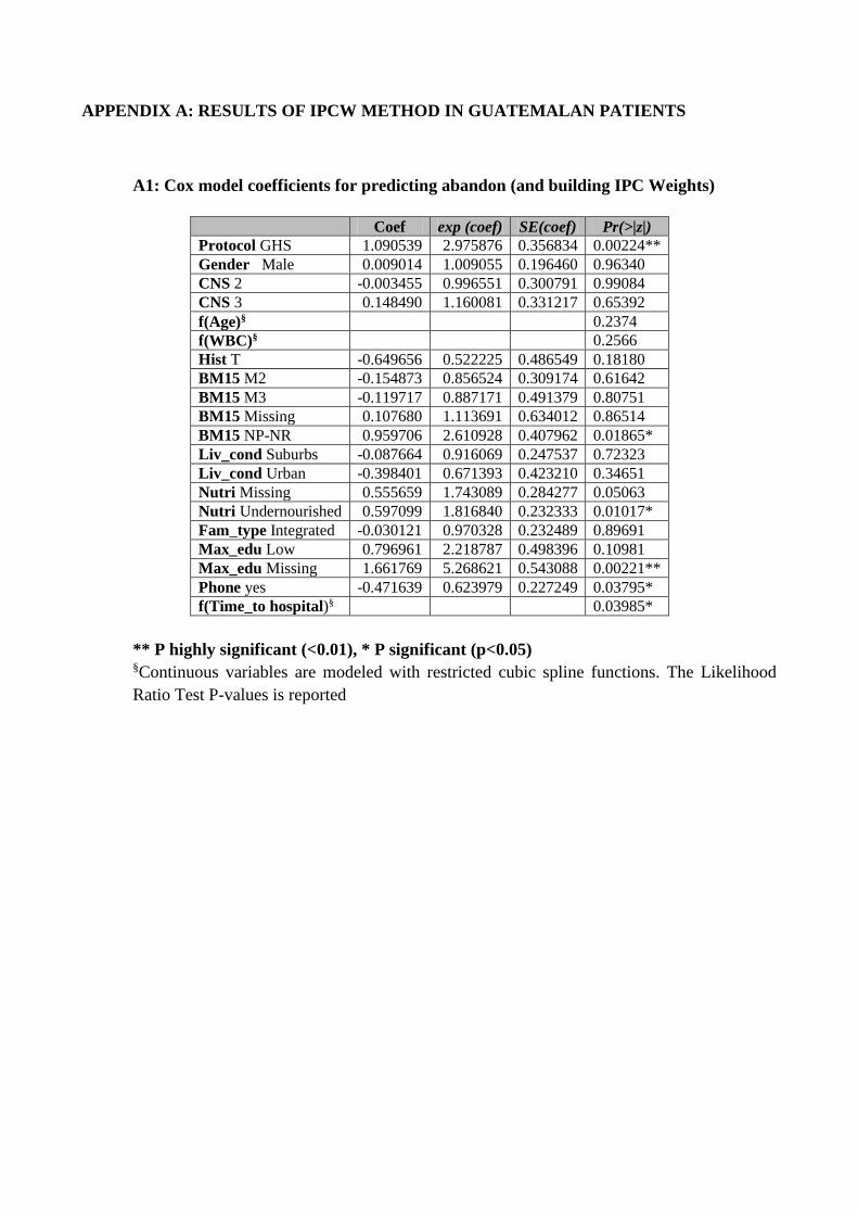
APPENDIX A: RESULTS OF IPCW METHOD IN GUATEMALAN PATIENTS

A1: Cox model coefficients for predicting abandon (and building IPC Weights)

Coef exp (coef) SE(coef) Pr(>|z|)

Protocol GHS 1.090539 2.975876 0.356834 0.00224**

Gender Male 0.009014 1.009055 0.196460 0.96340

CNS 2 -0.003455 0.996551 0.300791 0.99084

CNS 3 0.148490 1.160081 0.331217 0.65392

f(Age)§ 0.2374

f(WBC)§ 0.2566

Hist T -0.649656 0.522225 0.486549 0.18180

BM15 M2 -0.154873 0.856524 0.309174 0.61642

BM15 M3 -0.119717 0.887171 0.491379 0.80751

BM15 Missing 0.107680 1.113691 0.634012 0.86514

BM15 NP-NR 0.959706 2.610928 0.407962 0.01865*

Liv_cond Suburbs -0.087664 0.916069 0.247537 0.72323

Liv_cond Urban -0.398401 0.671393 0.423210 0.34651

Nutri Missing 0.555659 1.743089 0.284277 0.05063

Nutri Undernourished 0.597099 1.816840 0.232333 0.01017*

Fam_type Integrated -0.030121 0.970328 0.232489 0.89691

Max_edu Low 0.796961 2.218787 0.498396 0.10981

Max_edu Missing 1.661769 5.268621 0.543088 0.00221**

Phone yes -0.471639 0.623979 0.227249 0.03795*

f(Time_to hospital)§ 0.03985*

** P highly significant (<0.01), * P significant (p<0.05) §Continuous variables are modeled with restricted cubic spline functions. The Likelihood

Ratio Test P-values is reported

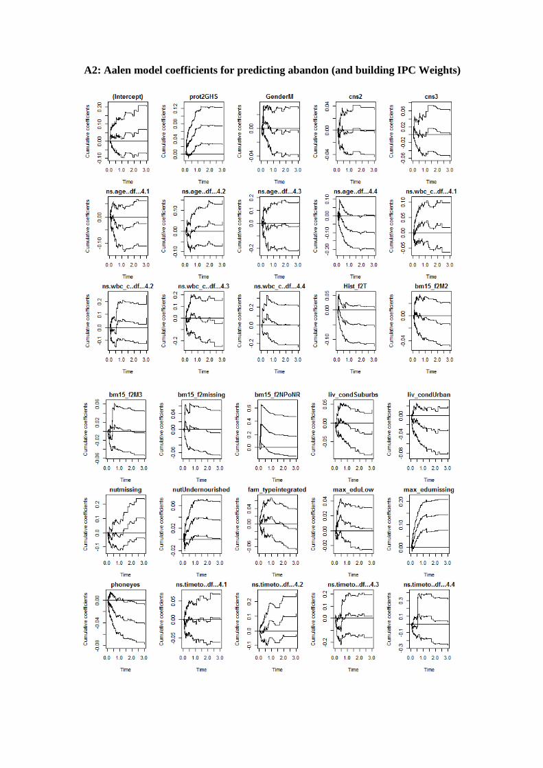
A2: Aalen model coefficients for predicting abandon (and building IPC Weights)

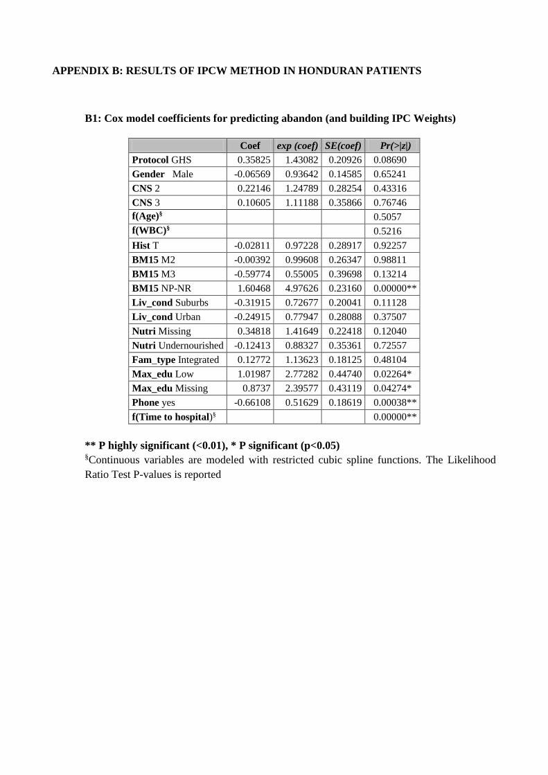
APPENDIX B: RESULTS OF IPCW METHOD IN HONDURAN PATIENTS

B1: Cox model coefficients for predicting abandon (and building IPC Weights)

Coef exp (coef) SE(coef) Pr(>|z|)

Protocol GHS 0.35825 1.43082 0.20926 0.08690

Gender Male -0.06569 0.93642 0.14585 0.65241

CNS 2 0.22146 1.24789 0.28254 0.43316

CNS 3 0.10605 1.11188 0.35866 0.76746

f(Age)§ 0.5057

f(WBC)§ 0.5216

Hist T -0.02811 0.97228 0.28917 0.92257

BM15 M2 -0.00392 0.99608 0.26347 0.98811

BM15 M3 -0.59774 0.55005 0.39698 0.13214

BM15 NP-NR 1.60468 4.97626 0.23160 0.00000**

Liv_cond Suburbs -0.31915 0.72677 0.20041 0.11128

Liv_cond Urban -0.24915 0.77947 0.28088 0.37507

Nutri Missing 0.34818 1.41649 0.22418 0.12040

Nutri Undernourished -0.12413 0.88327 0.35361 0.72557

Fam_type Integrated 0.12772 1.13623 0.18125 0.48104

Max_edu Low 1.01987 2.77282 0.44740 0.02264*

Max_edu Missing 0.8737 2.39577 0.43119 0.04274*

Phone yes -0.66108 0.51629 0.18619 0.00038**

f(Time to hospital)§ 0.00000**

** P highly significant (<0.01), * P significant (p<0.05) §Continuous variables are modeled with restricted cubic spline functions. The Likelihood

Ratio Test P-values is reported

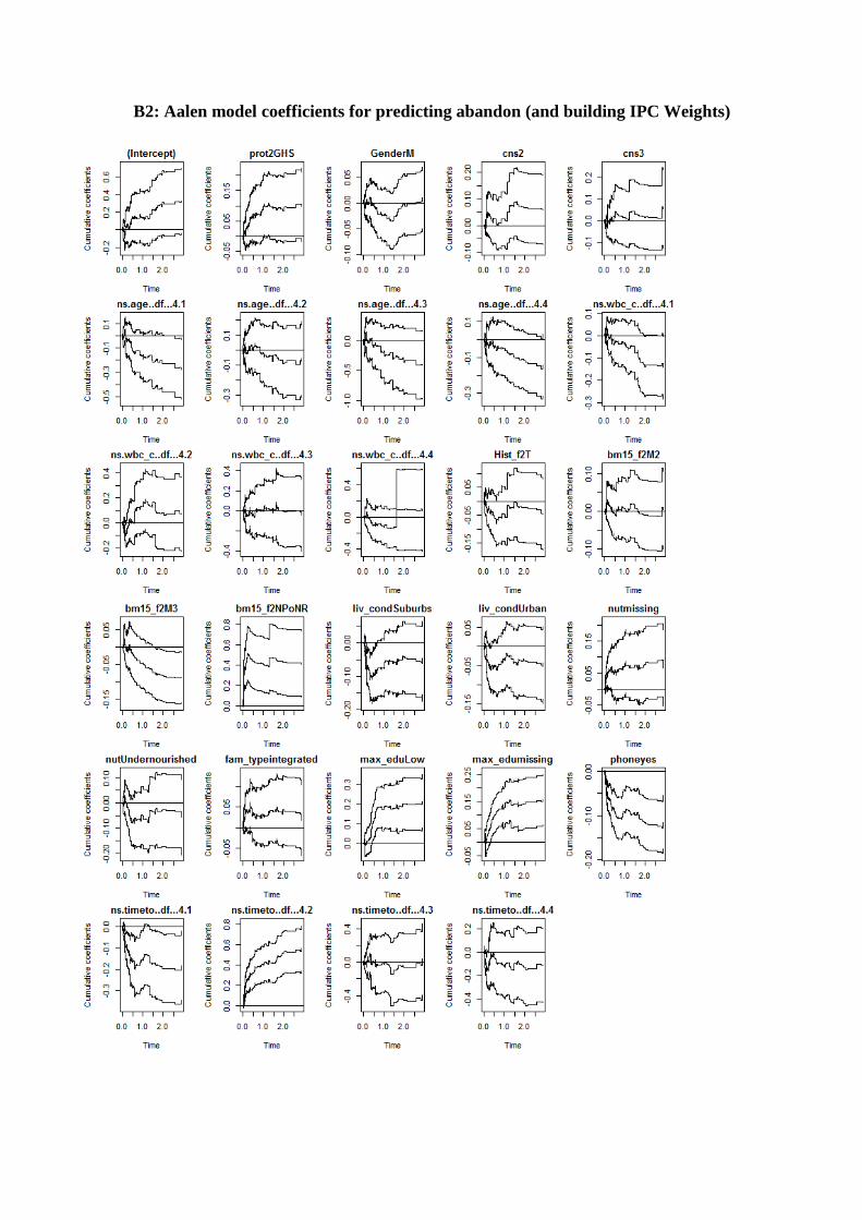
B2: Aalen model coefficients for predicting abandon (and building IPC Weights)

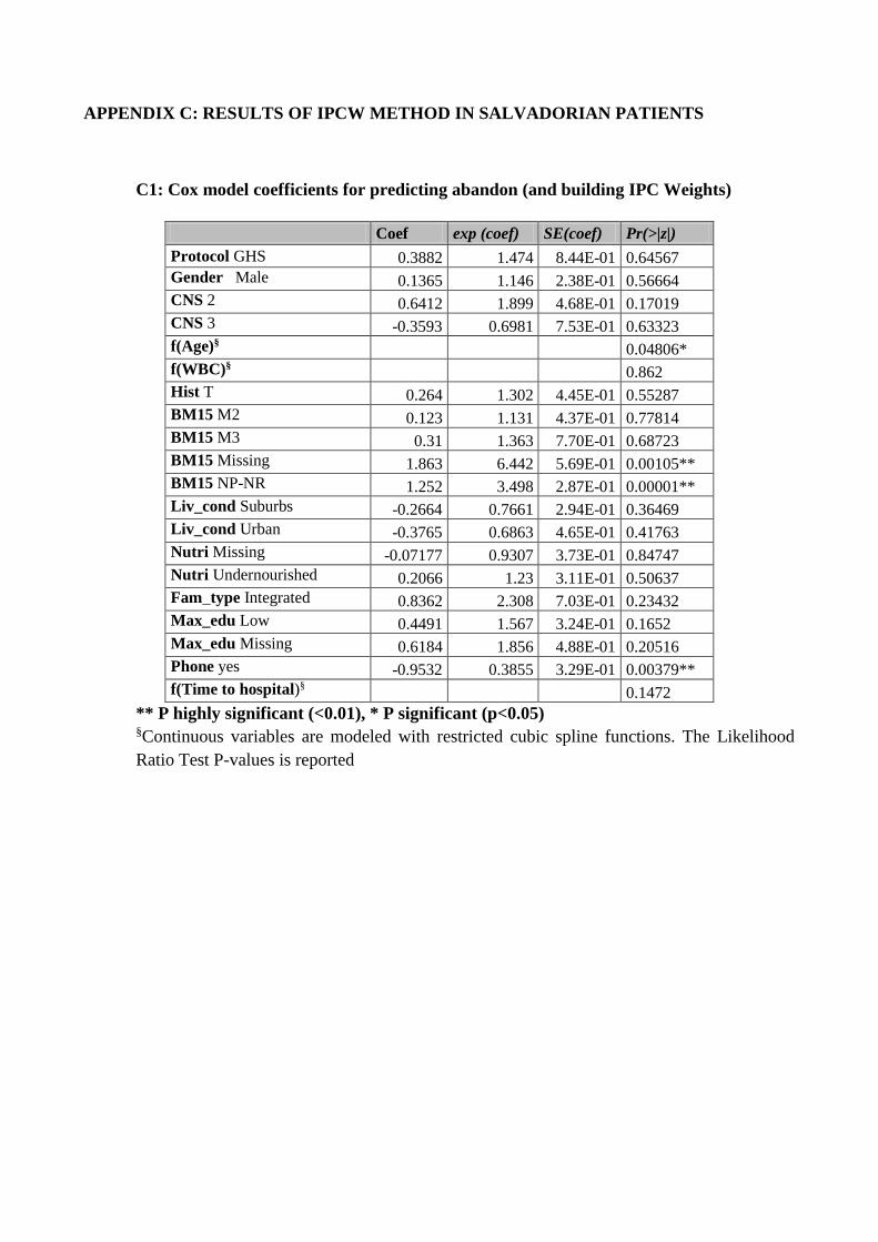
APPENDIX C: RESULTS OF IPCW METHOD IN SALVADORIAN PATIENTS

C1: Cox model coefficients for predicting abandon (and building IPC Weights)

Coef exp (coef) SE(coef) Pr(>|z|)

Protocol GHS 0.3882 1.474 8.44E-01 0.64567

Gender Male 0.1365 1.146 2.38E-01 0.56664

CNS 2 0.6412 1.899 4.68E-01 0.17019

CNS 3 -0.3593 0.6981 7.53E-01 0.63323

f(Age)§ 0.04806*

f(WBC)§ 0.862

Hist T 0.264 1.302 4.45E-01 0.55287

BM15 M2 0.123 1.131 4.37E-01 0.77814

BM15 M3 0.31 1.363 7.70E-01 0.68723

BM15 Missing 1.863 6.442 5.69E-01 0.00105**

BM15 NP-NR 1.252 3.498 2.87E-01 0.00001**

Liv_cond Suburbs -0.2664 0.7661 2.94E-01 0.36469

Liv_cond Urban -0.3765 0.6863 4.65E-01 0.41763

Nutri Missing -0.07177 0.9307 3.73E-01 0.84747

Nutri Undernourished 0.2066 1.23 3.11E-01 0.50637

Fam_type Integrated 0.8362 2.308 7.03E-01 0.23432

Max_edu Low 0.4491 1.567 3.24E-01 0.1652

Max_edu Missing 0.6184 1.856 4.88E-01 0.20516

Phone yes -0.9532 0.3855 3.29E-01 0.00379**

f(Time to hospital)§ 0.1472

** P highly significant (<0.01), * P significant (p<0.05) §Continuous variables are modeled with restricted cubic spline functions. The Likelihood

Ratio Test P-values is reported

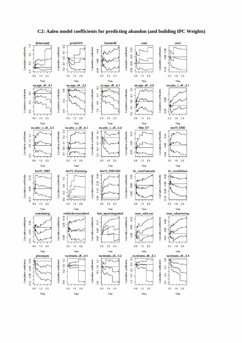
C2: Aalen model coefficients for predicting abandon (and building IPC Weights)