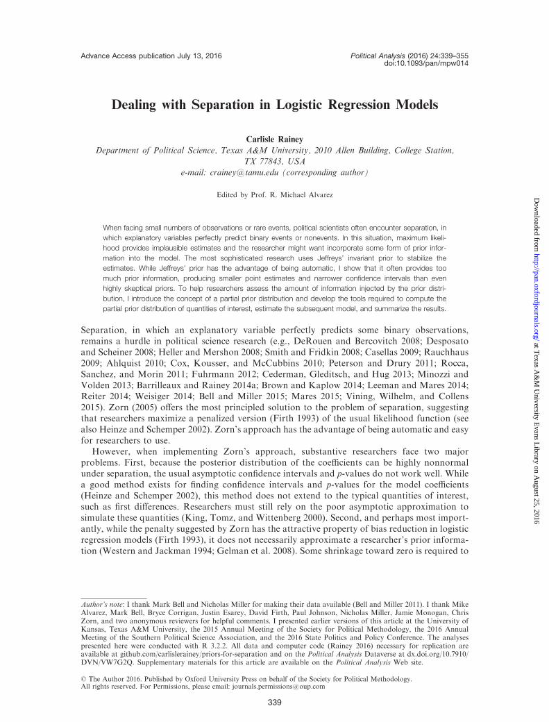
Dealing with Separation in Logistic Regression Models

Carlisle Rainey

Department of Political Science, Texas A&M University, 2010 Allen Building, College Station,

TX 77843, USA

e-mail: crainey@tamu.edu (corresponding author)

Edited by Prof. R. Michael Alvarez

When facing small numbers of observations or rare events, political scientists often encounter separation, in

which explanatory variables perfectly predict binary events or nonevents. In this situation, maximum likeli-

hood provides implausible estimates and the researcher might want incorporate some form of prior infor-

mation into the model. The most sophisticated research uses Jeffreys’ invariant prior to stabilize the

estimates. While Jeffreys’ prior has the advantage of being automatic, I show that it often provides too

much prior information, producing smaller point estimates and narrower confidence intervals than even

highly skeptical priors. To help researchers assess the amount of information injected by the prior distri-

bution, I introduce the concept of a partial prior distribution and develop the tools required to compute the

partial prior distribution of quantities of interest, estimate the subsequent model, and summarize the results.

Separation, in which an explanatory variable perfectly predicts some binary observations,remains a hurdle in political science research (e.g., DeRouen and Bercovitch 2008; Desposatoand Scheiner 2008; Heller and Mershon 2008; Smith and Fridkin 2008; Casellas 2009; Rauchhaus2009; Ahlquist 2010; Cox, Kousser, and McCubbins 2010; Peterson and Drury 2011; Rocca,Sanchez, and Morin 2011; Fuhrmann 2012; Cederman, Gleditsch, and Hug 2013; Minozzi andVolden 2013; Barrilleaux and Rainey 2014a; Brown and Kaplow 2014; Leeman and Mares 2014;Reiter 2014; Weisiger 2014; Bell and Miller 2015; Mares 2015; Vining, Wilhelm, and Collens2015). Zorn (2005) offers the most principled solution to the problem of separation, suggestingthat researchers maximize a penalized version (Firth 1993) of the usual likelihood function (seealso Heinze and Schemper 2002). Zorn’s approach has the advantage of being automatic and easyfor researchers to use.

However, when implementing Zorn’s approach, substantive researchers face two majorproblems. First, because the posterior distribution of the coefficients can be highly nonnormalunder separation, the usual asymptotic confidence intervals and p-values do not work well. Whilea good method exists for finding confidence intervals and p-values for the model coefficients(Heinze and Schemper 2002), this method does not extend to the typical quantities of interest,such as first differences. Researchers must still rely on the poor asymptotic approximation tosimulate these quantities (King, Tomz, and Wittenberg 2000). Second, and perhaps most import-antly, while the penalty suggested by Zorn has the attractive property of bias reduction in logisticregression models (Firth 1993), it does not necessarily approximate a researcher’s prior informa-tion (Western and Jackman 1994; Gelman et al. 2008). Some shrinkage toward zero is required to

Author’s note: I thank Mark Bell and Nicholas Miller for making their data available (Bell and Miller 2011). I thank MikeAlvarez, Mark Bell, Bryce Corrigan, Justin Esarey, David Firth, Paul Johnson, Nicholas Miller, Jamie Monogan, ChrisZorn, and two anonymous reviewers for helpful comments. I presented earlier versions of this article at the University ofKansas, Texas A&M University, the 2015 Annual Meeting of the Society for Political Methodology, the 2016 AnnualMeeting of the Southern Political Science Association, and the 2016 State Politics and Policy Conference. The analysespresented here were conducted with R 3.2.2. All data and computer code (Rainey 2016) necessary for replication areavailable at github.com/carlislerainey/priors-for-separation and on the Political Analysis Dataverse at dx.doi.org/10.7910/DVN/VW7G2Q. Supplementary materials for this article are available on the Political Analysis Web site.

Advance Access publication July 13, 2016 Political Analysis (2016) 24:339–355doi:10.1093/pan/mpw014

� The Author 2016. Published by Oxford University Press on behalf of the Society for Political Methodology.All rights reserved. For Permissions, please email: journals.permissions@oup.com

339

at Texas A

&M

University E

vans Library on A

ugust 25, 2016http://pan.oxfordjournals.org/

Dow

nloaded from

obtain finite estimates, but the appropriate amount of shrinkage depends on the substantiveproblem and the prior information. To address these two problems, I suggest that researchersuse a range of priors, focusing on an informative prior, and use MCMC to simulate directly fromthe posterior.

In this article, I introduce conceptual and computational tools that help researchers under-stand the information provided by a given prior distribution and use that prior distribution toobtain meaningful point estimates and confidence intervals. I make three specific contributions.First, I use statistical theory and two applied examples to demonstrate the importance ofchoosing a prior distribution that represents actual prior information and conducting robustnesschecks using a variety of prior distributions. Second, I introduce the concept of a partial priordistribution, a powerful tool in understanding and choosing a prior when facing separation.Third, I introduce new software that makes it easy for researchers to choose an informativeprior distribution, simulates directly from the posterior distribution, and summarizes theinferences.

I begin with a basic overview of the logistic regression model and summary of the impact ofseparation on the maximum likelihood estimates. I then describe two default prior distributionsthat researchers might use to handle separation. Next, I use a theoretical result and an appliedexample to demonstrate the importance of choosing an informative prior. I then introduce re-searchers to the concept of a partial prior distribution, which enables researchers to understandcomplex prior distributions in terms of the key quantities of interest. To illustrate how these ideaswork in practice, I conclude with a replication of Rauchhaus (2009) and Bell and Miller (2015),whose disagreement about the effect of nuclear weapons on war hinges, in part, on how to deal withseparation.

1 The Logistic Regression Model

Political scientists commonly use logistic regression to model the probability of events such as war(e.g., Fearon 1994), policy adoption (e.g., Berry and Berry 1990), turning out to vote (e.g.,Wolfinger and Rosenstone 1980), and government formation (e.g., Martin and Stevenson 2001).In the typical situation, the researcher uses an n� ðkþ 1Þ design matrix X consisting of a singlecolumn of ones and k explanatory variables to model a vector of n binary outcomes y, whereyi 2 f0; 1g, using the model PrðyiÞ ¼ Prðyi ¼ 1jXiÞ ¼

11þe�Xi�

, where � is a coefficient vector oflength kþ 1.

Using this model, it is straightforward to calculate the likelihood function

Prðyj�Þ ¼ Lð�jyÞ ¼Yni¼1

1

1þ e�Xi�

� �yi

1�1

1þ e�Xi�

� �1�yi" #

: ð1Þ

Researchers routinely obtain the maximum likelihood estimate �̂mle

of the coefficient vector � byfinding the coefficient vector that maximizes L (i.e., maximizing the likelihood of the observeddata). While this approach works quite well in most applications, it fails in a situation known asseparation (Zorn 2005).

2 Separation

Separation occurs in models of binary outcome data when one explanatory variable perfectlypredicts zeros, ones, or both.1 For a binary explanatory variable si (for separating explanatoryvariable), complete separation occurs when si perfectly predicts both zeros and ones.2 Quasicomplete

1Separation can also occur when a combination of explanatory variables perfectly predicts zeros, ones, or both; seeLesaffre and Albert (1989). See Geyer (2009) for a much more general view of the concept of separation.

2For simplicity, I describe complete and quasicomplete separation for a binary explanatory variable, which is moreexplicable than the general case considered by Albert and Anderson (1984). My approach also follows the convention ofHeinze and Schemper (2002) and Zorn (2005). Indeed, in social science problems, binary explanatory variables morecommonly lead to separation, so little is lost.

Carlisle Rainey340

at Texas A

&M

University E

vans Library on A

ugust 25, 2016http://pan.oxfordjournals.org/

Dow

nloaded from

separation occurs when si perfectly predicts either zeros or ones, but not both (Albert and Anderson1984; Zorn 2005). Overlap, the ideal case, occurs when there is no such si. With overlap, the usualmaximum likelihood estimates exist and provide reasonable estimates of parameters. However,under complete or quasicomplete separation, finite maximum likelihood estimates do not existand the usual method of calculating standard errors fails (Albert and Anderson 1984; Zorn 2005).

For the binary explanatory variable si, complete separation occurs when si perfectly predicts bothzeros and ones. For example, suppose si, such that yi¼ 0 for si¼ 0 and yi¼ 1 for si¼ 1. To maximizethe likelihood of the observed data, the “S”-shaped logistic regression curve must assignPrðyiÞ ¼

11þe�Xi�

¼ 0 when si ¼ 0 and PrðyiÞ ¼1

1þe�Xi�¼ 1 when si¼ 1. Since the logistic regression

curve lies strictly between zero and one, this likelihood cannot be achieved, only approached asymp-totically as the coefficient �s for si approaches infinity. Thus, the likelihood function under completeseparation is monotonic, which implies that a finite maximum likelihood estimate does not exist.

Quasicomplete separation occurs when si perfectly predicts either zeros or ones. For example,suppose that when si¼ 0, sometimes yi¼ 1 and other times yi¼ 0, but when si¼ 1, yi¼ 1 always. Tomaximize the likelihood of the observed data, the “S”-shaped logistic regression curve must assignPrðyiÞ ¼

11þe�Xi�

2 ð0; 1Þ when si ¼ 0 and PrðyiÞ ¼1

1þe�Xi�¼ 1 when si¼ 1. Again, since the logistic

regression curve lies strictly between zero and one, this likelihood cannot be achieved, only ap-proached asymptotically. Thus, the likelihood function under quasicomplete separation also mono-tonically increases as the coefficient of si increases, which again implies that the maximumlikelihood estimate does not exist.

For example, Barrilleaux and Rainey (2014a) find that no Democratic governors opposed theMedicaid expansion under the Affordable Care Act (ACA), leading to a maximum likelihoodestimate of negative infinity for the coefficient of the indicator of Democratic governors.Similarly, Rauchhaus (2009) and Bell and Miller (2015) finds no instances of states with nuclearweapons engaging in war with each other, leading to an estimated coefficient of negative infinity forthe coefficient of the variable indicating nuclear dyads. To maximize the likelihood in these situ-ations, the model must assign zero probability of opposition to Democratic governors and zeroprobability of war to nuclear dyads. Because the logistic regression curve lies strictly above zero,this cannot happen, though it can be approached asymptotically as the coefficient of si goes tonegative infinity.

For convenience, I say that the “direction of the separation” is positive if and only if si ¼ 1)yi ¼ 1 or si ¼ 0) yi ¼ 0 and that the direction of separation is negative if and only if si ¼ 0)yi ¼ 1 or si ¼ 1) yi ¼ 0. Thus, �̂

mle¼ þ1 when the direction of the separation is positive, and

�̂mle¼ �1 when the direction of the separation is negative.

3 Solutions to Separation

The maximum likelihood framework requires the researcher to find the parameter vector that“maximizes the likelihood of the observed data.” Of course, infinite coefficients always generateseparated data, whereas finite coefficients only sometimes generate separation. Thus, under separ-ation, maximum likelihood can only produce infinite estimates.

Before addressing potential solutions to this problem, let me mention two unsatisfactory “solu-tions” found in applied work. In some cases, researchers simply ignore the problem of separationand interpret the large estimates and standard errors as though these are reasonable. However, thisapproach leads researchers to overstate the magnitude of the effect and the uncertainty of theestimates. Second, researchers sometimes “solve” the problem of separation by dropping theseparating variable from the model. Zorn (2005, 161–62) correctly dismisses this approach:

As a practical matter, separation forces the analyst to choose from a number of problematic alternatives for

dealing with the problem. The most widely used “solution” is simply to omit the offending variable or

variables from the analysis. In political science, this is the approach taken in a number of studies in

international relations, comparative politics, and American politics. It is also the dominant approach in

sociology, economics, and the other social sciences, and it is the recommended method in a few prominent

texts in statistics and econometrics. Of course, this alternative is a particularly unattractive one; omitting a

covariate that clearly bears a strong relationship to the phenomenon of interest is nothing more than

deliberate specification bias.

Separation in Logistic Regression Models 341

at Texas A

&M

University E

vans Library on A

ugust 25, 2016http://pan.oxfordjournals.org/

Dow

nloaded from

One principled solution is to build prior information pð�Þ—the same prior information that leadsresearchers to deem infinite coefficients “implausibly large”—into the model using Bayes’ rule, sothat

pð�jyÞ ¼pðyj�Þzfflffl}|fflffl{likelihood

pð�Þz}|{prior

Rpðyj�Þpð�Þd�

: ð2Þ

In this case, the estimate switches from the maximum likelihood estimate to a summary of thelocation of the posterior distribution, such as the posterior median. The current literature ondealing with separation suggests researcher take an automatic approach by using a default priordistribution, such as Jeffreys’ invariant prior distribution (Jeffreys 1946; Zorn 2005) or a heavy-tailed Cauchy(0, 2.5) prior distribution (Gelman et al. 2008).

3.1 Jeffreys’ Invariant Prior

Zorn (2005) suggests that political scientists deal with separation by maximizing a penalized like-lihood rather than the likelihood (see Heinze and Schemper 2002 as well). Zorn suggests replacingthe usual likelihood function Lð�jyÞ with the “penalized” likelihood function L�ð�jyÞ from Firth(1993), so that L�ð�jyÞ ¼ Lð�jyÞjIð�Þj

12. It turns out that the penalty jIð�Þj

12 is equivalent to Jeffreys’

(1946) prior for the logistic regression model (Firth 1993; Poirier 1994). Jeffreys’ prior can beobtained by applying Jeffreys’ rule (Jeffreys 1946; Box and Taio 2011, 41–60), which requiressetting the prior pð�Þ to be proportional to the square root of the determinant of the informationmatrix, so that pð�Þ / jIð�Þj

12. Then, of course, applying Bayes’ rule yields the posterior distribution

pð�jyÞ / Lð�jyÞjIð�Þj12, so that Firth’s penalized likelihood is equivalent to a Bayesian approach with

Jeffreys’ prior. The researcher can then sample from this posterior distribution using MCMC toobtain the features of interest, such as the mean and standard deviation.

However, Firth (1993) did not propose this prior to solve the separation problem. Instead, heproposed using Jeffreys’ prior to reduce the well-known small sample bias in logistic regressionmodels. And while it is true that Firth’s correction does provide finite estimates under separation, itremains an open question whether this automatic prior, justified on other grounds, injects a rea-sonable amount of information into the model for particular substantive applications. In somecases, Jeffreys’ prior might contain too little information. In other cases, it might contain too much.

3.2 The Cauchy(0, 2.5) Prior

Indeed, Gelman et al. (2008) note that Firth’s application of Jeffreys’ prior is not easily interpret-able as actual prior information because the prior pð�Þ ¼ jIð�Þj

12 lacks an interpretable scale and

depends on the data in complex ways. Instead, they suggest standardizing continuous inputs tohave mean zero and standard deviation one-half and simply centering binary inputs (Gelman 2008).Then, they suggest placing a weakly informative Cauchy(0, 2.5) prior on the coefficients for theserescaled variables that, like Jeffreys’ prior, bounds the estimates away from positive and negativeinfinity but can also be interpreted as actual prior information.3 Gelman et al. (2008, 1363) write:

Our key idea is that actual effects tend to fall within a limited range. For logistic regression, a change of 5

moves a probability from 0.01 to 0.5, or from 0.5 to 0.99. We rarely encounter situations where a shift in input

x corresponds to the probability of outcome y changing from 0.01 to 0.99, hence, we are willing to assign a

prior distribution that assigns low probabilities to changes of 10 on the logistic scale.

As with Jeffreys’ prior, the posterior distribution is not easily available analytically, but one canuse MCMC to simulate from the posterior distribution. Once a researcher has the MCMC

3Gelman et al. (2008) use a Cauchy(0, 2.5) prior for the coefficients but a Cauchy(0, 10) prior for the intercept. Thisallows the intercept to take on a much larger range of values (e.g., from 10�9 to 1� 10�9).

Carlisle Rainey342

at Texas A

&M

University E

vans Library on A

ugust 25, 2016http://pan.oxfordjournals.org/

Dow

nloaded from

simulations, she can obtain the point estimates and credible intervals for the coefficients orquantities of interest by summarizing the simulations.

Gelman et al. (2008) design their prior distribution to be reflective of prior information for arange of situations. In many cases, their weakly informative prior might supply too little priorinformation. In other cases, it might supply too much. In either case, it remains an open questionwhether this general prior supplies appropriate information for particular research problems.

4 The Importance of the Prior

While default priors, such as Zorn’s suggested Jeffreys’ prior or Gelman et al.’s suggested Cauchy(0,2.5) prior are often useful as starting points, choosing an informative prior distribution is crucial fordealing with separation in a substantively meaningful manner. Further, whether a particular prioris reasonable depends on the particular application.

In most data analyses, the data swamp the contribution of the prior, so that the choice of priorhas little effect on the posterior. However, in the case of separation, the prior essentially determinesthe shape of the posterior in the direction of the separation. When dealing with separation, then, theprior distribution is not an arbitrary choice made for computational convenience, but an importantchoice that affects the inferences. We can see the importance in both theory and practice.

4.1 The Impact of the Prior in Theory

Although it is intuitive that the prior drives the inferences in the direction of the separation, it isalso easy to generally characterize the impact of the prior on a monotonically increasing likelihood.Suppose quasicomplete separation, such that whenever an explanatory variable si¼ 1, a binaryoutcome yi¼ 1, but when si¼ 0, yi might equal zero or one. Suppose further that the analystwishes to obtain plausible estimates of coefficients for the model

Prðyi ¼ 1Þ ¼ logit�1ð�cons þ �ssi þ �1xi1 þ �2xi2 þ :::þ �kxikÞ: ð3Þ

It is easy to find plausible estimates for the coefficients of x1; x2; :::; xk using maximum likeli-hood, but finding a plausible estimate of �s proves more difficult because maximum likelihoodsuggests an estimate of þ1. In order to obtain a plausible estimate of �s, the researcher mustintroduce prior information into the model. My purpose here is to characterize how this priorinformation impacts the posterior distribution.

In the general situation, the analyst is interested in computing and characterizing the posteriordistribution of �s given the data. Using Bayes’ rule, the posterior distribution of � ¼ h�cons; �s; �1;�2; :::; �ki depends on the likelihood and the prior, so that pð�jyÞ / pðyj�Þpð�Þ. In particular, theanalyst might have in mind a family of priors centered at and monotonically decreasing away fromzero with varying scale �, so that pð�sÞ ¼ pð�sjsÞ, though the results below simply depend on havingany proper prior distribution. The informativeness of the prior distribution depends on �, which ischosen by the researcher and “flattens” the prior pð�sÞ ¼ pð�sjsÞ, such that as � increases, the rate atwhich the prior descends to zero decreases. In practice, one uses � to control the amount of shrink-age. A small � produces more shrinkage; a large � produces less.

Theorem 1. For a monotonic likelihood pðyj�Þ increasing [decreasing] in �s, proper prior distributionpð�jsÞ, and large positive [negative] �s, the posterior distribution of �s is proportional to the priordistribution for �s, so that pð�sjyÞ / pð�sjsÞ. More formally, lim �s!1

½�1�

pð�sjyÞpð�sjsÞ

¼ k, for postive constant k.

Proof and details: See the Supplementary Technical Appendix.

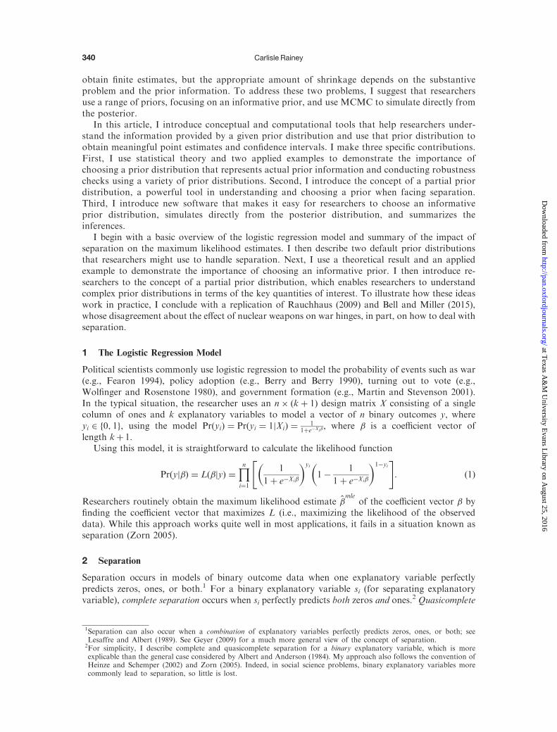
Figure 1 provides the intuition of Theorem 1. In the top panel, we can easily see that multiplyingthe likelihood times the prior, as required by Bayes’ rule, causes the likelihood to determine theinferences in the direction opposite the separation and causes the prior to determine the inferencesin the direction of the separation. Notice that the right-hand side of the posterior barely changes as

Separation in Logistic Regression Models 343

at Texas A

&M

University E

vans Library on A

ugust 25, 2016http://pan.oxfordjournals.org/

Dow

nloaded from

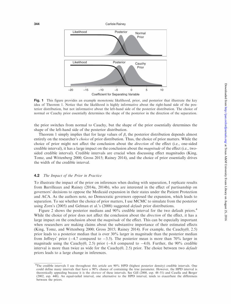
the prior switches from normal to Cauchy, but the shape of the prior essentially determines theshape of the left-hand side of the posterior distribution.

Theorem 1 simply implies that for large values of �s the posterior distribution depends almostentirely on the researcher’s choice of prior distribution. Thus, the choice of prior matters. While thechoice of prior might not affect the conclusion about the direction of the effect (i.e., one-sidedcredible interval), it has a large impact on the conclusion about the magnitude of the effect (i.e., two-sided credible interval). Credible intervals are crucial when discussing effect magnitudes (King,Tomz, and Wittenberg 2000; Gross 2015; Rainey 2014), and the choice of prior essentially drivesthe width of the credible interval.

4.2 The Impact of the Prior in Practice

To illustrate the impact of the prior on inferences when dealing with separation, I replicate resultsfrom Barrilleaux and Rainey (2014a, 2014b), who are interested in the effect of partisanship ongovernors’ decisions to oppose the Medicaid expansion in their states under the Patient Protectionand ACA. As the authors note, no Democratic governors opposed the expansion, which leads toseparation. To see whether the choice of prior matters, I use MCMC to simulate from the posteriorusing Zorn’s (2005) and Gelman et al.’s (2008) suggested default prior distributions.

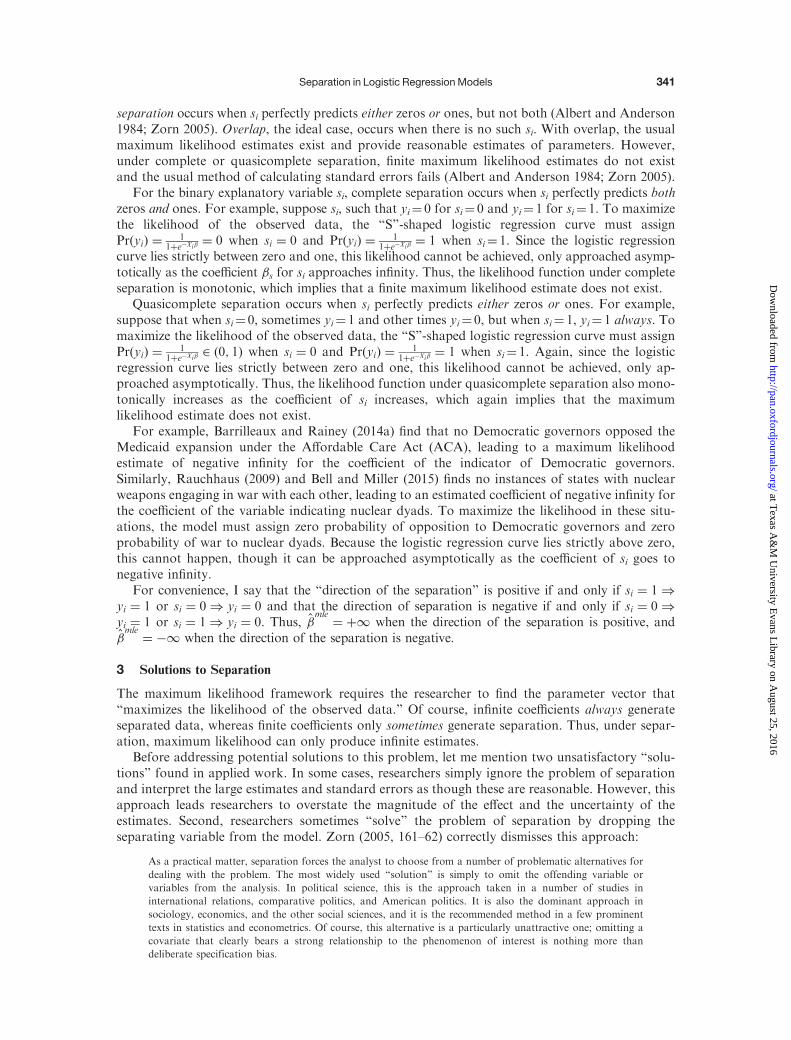
Figure 2 shows the posterior medians and 90% credible interval for the two default priors.4

While the choice of prior does not affect the conclusion about the direction of the effect, it has alarge impact on the conclusion about the magnitude of the effect. This can be especially importantwhen researchers are making claims about the substantive importance of their estimated effects(King, Tomz, and Wittenberg 2000; Gross 2015; Rainey 2014). For example, the Cauchy(0, 2.5)prior leads to a posterior median that is over 30% larger in magnitude than the posterior medianfrom Jeffreys’ prior (�4.7 compared to �3.5). The posterior mean is more than 70% larger inmagnitude using the Cauchy(0, 2.5) prior (�6.8 compared to �4.0). Further, the 90% credibleinterval is more than twice as wide for the Cauchy(0, 2.5) prior. The choice between two defaultpriors leads to a large change in inferences.

Likelihood NormalPrior

Posterior

−20 −15 −10 −5 0 5 10

Coefficient for Separating Variable

Likelihood CauchyPrior

Posterior

Fig. 1 This figure provides an example monotonic likelihood, prior, and posterior that illustrate the keyidea of Theorem 1. Notice that the likelihood is highly informative about the right-hand side of the pos-

terior distribution, but not informative about the left-hand side of the posterior distribution. The choice ofnormal or Cauchy prior essentially determines the shape of the posterior in the direction of the separation.

4The credible intervals I use throughout this article are 90% HPD (highest posterior density) credible intervals. Onecould define many intervals that have a 90% chance of containing the true parameter. However, the HPD interval istheoretically appealing because it is the shortest of these intervals. See Gill (2008, esp. 48–51) and Casella and Berger(2002, esp. 448). An equal-tailed interval, one alternative to the HPD interval, tends to exacerbate the differencesbetween the priors.

Carlisle Rainey344

at Texas A

&M

University E

vans Library on A

ugust 25, 2016http://pan.oxfordjournals.org/

Dow

nloaded from

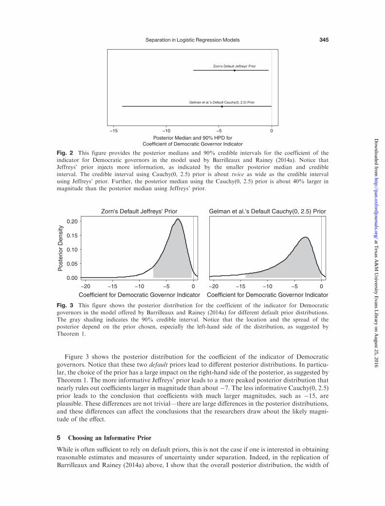
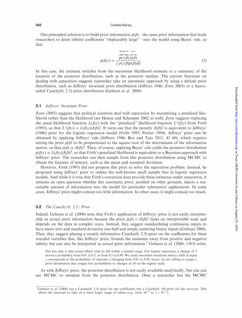
Figure 3 shows the posterior distribution for the coefficient of the indicator of Democraticgovernors. Notice that these two default priors lead to different posterior distributions. In particu-lar, the choice of the prior has a large impact on the right-hand side of the posterior, as suggested byTheorem 1. The more informative Jeffreys’ prior leads to a more peaked posterior distribution thatnearly rules out coefficients larger in magnitude than about �7. The less informative Cauchy(0, 2.5)prior leads to the conclusion that coefficients with much larger magnitudes, such as �15, areplausible. These differences are not trivial—there are large differences in the posterior distributions,and these differences can affect the conclusions that the researchers draw about the likely magni-tude of the effect.

5 Choosing an Informative Prior

While is often sufficient to rely on default priors, this is not the case if one is interested in obtainingreasonable estimates and measures of uncertainty under separation. Indeed, in the replication ofBarrilleaux and Rainey (2014a) above, I show that the overall posterior distribution, the width of

−20 −15 −10 −5 0

Coefficient for Democratic Governor Indicator

0.00

0.05

0.10

0.15

0.20

Pos

terio

r D

ensi

ty

Zorn's Default Jeffreys' Prior

−20 −15 −10 −5 0

Coefficient for Democratic Governor Indicator

Gelman et al.'s Default Cauchy(0, 2.5) Prior

Fig. 3 This figure shows the posterior distribution for the coefficient of the indicator for Democratic

governors in the model offered by Barrilleaux and Rainey (2014a) for different default prior distributions.The gray shading indicates the 90% credible interval. Notice that the location and the spread of theposterior depend on the prior chosen, especially the left-hand side of the distribution, as suggested byTheorem 1.

Fig. 2 This figure provides the posterior medians and 90% credible intervals for the coefficient of theindicator for Democratic governors in the model used by Barrilleaux and Rainey (2014a). Notice thatJeffreys’ prior injects more information, as indicated by the smaller posterior median and credible

interval. The credible interval using Cauchy(0, 2.5) prior is about twice as wide as the credible intervalusing Jeffreys’ prior. Further, the posterior median using the Cauchy(0, 2.5) prior is about 40% larger inmagnitude than the posterior median using Jeffreys’ prior.

Separation in Logistic Regression Models 345

at Texas A

&M

University E

vans Library on A

ugust 25, 2016http://pan.oxfordjournals.org/

Dow

nloaded from

the 90% credible interval, and the posterior median largely depend on the prior one chooses. Thisimplies that researchers relying on default priors alone risk under- or overrepresenting their con-fidence in the magnitude of the effect.

Data with separation fall into the category of “weak data” discussed by Western and Jackman(1994)—data that “provide little information about parameters of statistical models.” Under sep-aration, the data simply offer no information about the upper bound of the magnitude of thecoefficient of the separating variable. Any reasonable regularization, then, must come in theform of an informative prior. But a researcher’s prior is not simply a spur-of-the-momentfeeling. Instead, we should think of the prior as representing other information relevant to theestimation. This information can come from several sources, including quantitative studies ofsimilar topics, detailed analyses of particular cases, and theoretical arguments. As Western andJackman (1994, 415) note:

While extra quantitative information is typically unavailable, large and substantively rich stores of qualitative

information from comparative and historical studies are often present but not available in a form suitable for

analysis. Bayesian procedures enable weak quantitative information of comparative research to be pooled

with the qualitative information to obtain sharper estimates of the regression coefficients.

The best sources of prior information, though, depend on the substantive prior. The judgment ofthe substantive researcher, based on their understanding of the substantive problem, is crucial.

When facing separation, I suggest researchers use a prior distribution that satisfies threeproperties:

1. Shrinks the estimates toward zero. While the ultimate goal is to choose a prior distributionbased on actual prior information, the prior distribution should also be appropriately con-servative. As mentioned before, the prior distribution largely drives the inferences in thedirection of the separation. In this case, a noncentral prior distribution in the direction ofthe separation has an especially large impact on the inferences. For this reason, I focus onprior distributions centered at zero to conservatively shrink coefficients toward zero(Gelman and Jakulin 2007). The only choice the researcher needs to make is the amountof shrinkage appropriate for a given substantive problem.

2. Allows plausible effects. The prior distribution should assign substantial prior probability toestimates that are a priori plausible according to the researcher’s prior information.

3. Rules out implausibly large effects. The prior distribution should assign little prior probabil-ity to estimates that are a priori implausible according to the researcher’s prior information.

Different researchers will inevitably have different prior beliefs. For example, there is substantialdisagreement among international relations theorists about the likely effects of nuclear weapons onconflict. Some optimists believe that nuclear weapons make peace much more likely. Mearsheimer(1993, 57) argues that “nuclear weapons are a powerful force for peace” and observes:

In the pre-nuclear world of industrialized great powers, there were two world wars between 1900 and 1945 in which

some 50 million Europeans died. In the nuclear age, the story is very different. Only some 15,000 Europeans were

killed in minor wars between 1945 and 1990, and there was a stable peace between the superpowers that became

increasingly robust over time. A principal cause of this “long peace” was nuclear weapons.

Bueno de Mesquita and Riker (1982, 283) even theorize that the probability of conflict “decreasesto zero when all nations are nuclearly armed.”

On the other hand, some pessimists (e.g., Sagan 1994) believe that nuclear weapons do not deterconflict, only make it more catastrophic. Mueller (1988, 68–69) writes:

Nuclear weapons may well have enhanced this stability—they are certainly dramatic reminders of how

horrible a big war could be. But it seems highly unlikely that, in their absence, the leaders of the major powers

would be so unimaginative as to need such reminding. Wars are not begun out of casual caprice or idle fancy,

but because one country or another decides that it can profit from (not simply win) the war—the combination

of risk, gain, and cost appears to be preferable to peace. Even allowing considerably for stupidity, ineptness,

miscalculation, and self-deception in these considerations, it does not appear that a large war, nuclear or

otherwise, has been remotely in the interest of essentially-contented, risk-averse, escalation-anticipating

powers that have dominated world affairs since 1945.

Carlisle Rainey346

at Texas A

&M

University E

vans Library on A

ugust 25, 2016http://pan.oxfordjournals.org/

Dow

nloaded from

The optimists and the pessimists have different prior beliefs about the likely effects of nuclearweapons. These different beliefs must lead to different interpretations of the evidence because theprior distribution has such a strong impact on the posterior distribution in the direction of theseparation. Because of this, researchers must clearly communicate the dependence of the inferenceson the choice of prior by transparently developing an informative prior distribution and providingthe inferences for alternative prior beliefs.

However, choosing a prior distribution is quite difficult, especially for multidimensionalproblems. Gill and Walker (2005) provide an overview of methods of choosing a prior appropriateto social science research. However, the most sensible approach for choosing a prior distributiondepends on the nature of the statistical model and the prior information.

In general, the researcher might assess the reasonableness of the prior distribution by examiningthe prior distribution and asking herself whether the prior and model produce a distribution for thequantities of interest that matches her prior information. Under the Bayesian framework, the re-searcher has a fully specified model pnew ¼ pðynewj�Þpð�Þ and can simulate the quantity of interestqnew ¼ qðpnewÞ from the model prior to observing the data. This works much like the Clarify algorithm(King, Tomz, and Wittenberg 2000). By repeatedly simulating from the prior distribution ~� � pð�Þ,calculating ~pnew ¼ pðynewj ~�Þ, and calculating ~qnew ¼ qð ~pnewÞ, the researcher can recover the trans-formed prior distribution of qnew. Just as a researcher can use simulation to interpret the coefficientestimates of nonlinear models, she can use simulation to interpret the prior distribution.

This simulation is entirely pre-data. The researcher does not need to fit the model to data tosimulation the quantities of interest. Instead, she can simulate from the prior distribution (ratherthan the posterior), and use these prior simulations to interpret the prior distribution.

However, it is difficult to work with more than one dimension of the prior distribution.Specifying the full prior distribution requires simultaneously choosing prior distributions for thecoefficients of the kþ 1 explanatory variables, as well as the relationships among these coefficients(e.g., family, location, scale, and correlations of each coefficient). This process is intractably tedious,because the researcher must evaluate the prior for each combination of each parameter set at arange of values. Even if the researcher considers only independent normal priors centered at zeroand only ten values for each scale, then the researcher must examine 10kþ1 prior distributions. If theresearcher has eight control variables, so that k¼ 8 (e.g., Barrilleaux and Rainey 2014a), then theresearcher must evaluate one billion prior distributions.

But only specific regions of the kþ 1 dimensional prior distribution are practically importantwhen addressing separation. This allows the researcher to dramatically simplify the choice of prior.In particular, the researcher can simplify the focus in two specific ways.

1. Focus only on the separated coefficient. Since the data swamp the prior for all the modelcoefficients except �s, the only relevant “slices” of the prior distribution are those in whichall other coefficients are near their maximum likelihood estimates.

2. Focus in the direction of the separation. The likelihood also swamps the prior in the directionopposite the separation. Unless the researcher has an extremely small data set [i.e., smallerthan Barrilleaux and Rainey (2014a), who have n¼ 50], then the likelihood essentially rulesout values less [greater] than zero when the direction of separation is positive [negative].

I refer to this simplified focus as the partial prior distribution.Formally, we might write the partial prior distribution as p�ð�sj�s � 0; ��s ¼ �̂

mle

�s Þ when

�̂mle

s ¼ þ1 and p�ð�sj�s � 0; ��s ¼ �̂mle

�s Þ when �̂mle

s ¼ �1. Much like the researcher can recover

the prior distribution of qnew implied by the prior distribution, she can recover the distribution of qnewimplied by the partial prior distribution by repeatedly simulating from the partial prior distribution

~��� p�ð�sj�s � 0; ��s ¼ �̂

mle

�s Þ, calculating ~p�new ¼ pðynewj ~��Þ, and calculating ~q�new ¼ qð ~p�newÞ.

The researcher should only use the partial prior distribution to study and interpret the priordistribution, not to estimate the model. For estimating the model, researchers should use the fullprior distribution described below in Section 6.

This process requires the researcher to use the data twice—an initial fit using maximum likeli-hood and a final fit using MCMC. First, the researcher fits the model using maximum likelihood to

Separation in Logistic Regression Models 347

at Texas A

&M

University E

vans Library on A

ugust 25, 2016http://pan.oxfordjournals.org/

Dow

nloaded from

obtain a reasonable estimate of the coefficients or the nonseparating explanatory variables (uponwhich the quantities of interest depend). The maximum likelihood estimation produces an estimateof &1 for the coefficient of the separation variable; this is akin to excluding the perfectlypredicted cases from the analysis or using the imperfectly predicted cases to estimate the coefficientsof the nonseparated explanatory variables. For example, even though no Democratic governorsopposed the Medicaid expansion, Barrilleaux and Rainey (2014a) can use the Republican states toestimate the coefficients for their other explanatory variables, including the percentage of the state’sresidents who feel favorable toward the ACA, whether Republicans control the state legislature, thepercentage of the state that is uninsured, and others. This initial maximum likelihood estimationonly serves to identify the especially important region of the (multivariate) prior distribution: thedimension for the coefficient of the separating explanatory variable in the direction of the separ-ation with the other coefficients near their maximum likelihood estimates.

For example, Barrilleaux and Rainey (2014a) do not need to use prior information to obtainreasonable estimates for their measures of need and public opinion. Further, because noDemocratic governors opposed the Medicaid expansion, they do not need the prior to rule outlarge positive effects for Democratic partisanship. In these cases, the likelihood is sufficiently in-formative. However, Barrilleaux and Rainey (2014a) do need to use the prior to rule out largenegative effects for Democratic partisanship, because the likelihood cannot effectively rule outimplausibly large negative effects. Indeed, the likelihood is monotonically decreasing in the coeffi-cient of the indicator of Democratic governors. That is, the likelihood increases as the coefficient ofDemocratic partisanship becomes more negative. The larger the negative effect, the more likelyseparation would occur. The usual maximum likelihood estimator, therefore, provides implausiblylarge negative estimates and unreasonable standard errors. Theorem 1 provides a more formaltreatment of this intuition, but prior information is essential to obtain reasonable estimates andmeasures of uncertainty.

Choosing a prior, though, requires thoughtful effort. As I show above, default priors can lead tomuch different conclusions, so it is essential to build actual prior information into the model. Inorder to choose a reasonable, informative prior distribution, researchers can use simulation toobtain the partial prior distribution of the quantity of interest. The following steps describe howresearchers can simulate from the partial prior distribution of a quantity of interest and use thesimulations to check the reasonableness of the choice.

1. Estimate the model coefficients using maximum likelihood, giving the coefficient vector �̂mle

.Include the separating variable si in the model. Of course, this leads to implausible estimatesfor �s, but the purpose is to choose reasonable values at which to fix the other coefficients inorder to focus on a single slice of the full prior.

2. Choose a prior distribution pð�sjsÞ for the separating variable s that is centered at zero withscale parameter �. One sensible choice is the scaled t distribution, which has the normal andCauchy families as special cases (df ¼ 1 and df ¼ 1, respectively).

3. Choose a large number of simulations nsims to perform (e.g., nsims � 10; 000) and for i in 1to nsims, do the following:

(a) Simulate ~�½i�

s � pð�sÞ.

(b) Replace �̂mle

s in �̂mle

with ~�½i�

s , yielding the vector ~�½i�.

(c) Calculate and store the quantity of interest ~q½i� ¼ q ~�½i�

� �. This quantity of interest might

be a first-difference or risk ratio, for example.

4. Keep only those simulations in the direction of the separation (e.g., ~�½i�

s � 0 when �̂mle

s ¼ þ1

and ~�½i�

s � 0 when �̂mle

s ¼ �1).5

5In some situations, researchers may wish to skip this step. For example, if the numbers of perfectly predicted cases (e.g.,states with Democratic governors or nuclear dyads) are relatively few, then the researchers can skip this step to evaluatethe prior in the direction of the separation as well as the opposite direction. However, a scale parameter that produces

Carlisle Rainey348

at Texas A

&M

University E

vans Library on A

ugust 25, 2016http://pan.oxfordjournals.org/

Dow

nloaded from

5. Summarize the simulations ~q using quantiles, histograms, or density plots. If the prior is inad-equate, then update the prior distribution pð�sjsÞ by choosing a larger or smaller value of �.

Given that the inference can be highly dependent on the choice of prior, I recommend that theresearcher choose at least three prior distributions: (1) an informative prior distribution that rep-resents her actual information, (2) a highly skeptical prior distribution that suggests the effect islikely small, and (3) a highly enthusiastic prior that suggests the effect might be very large. Indeed,Western and Jackman (1994, 422) note:

Still, the subjective choice of prior is an important weakness of Bayesian practice. The consequences of this

weakness can be limited by surveying the sensitivity of conclusions to a broad range of prior beliefs and to

subsets of the sample.

Combined with Zorn’s (2005) and Gelman et al.’s (2008) suggested defaults, these provide a rangeof prior distributions that the researcher can use to evaluate her inferences.

6 Estimating the Full Model

Once the researcher obtains a reasonable prior distribution as well as several to use for robustnesschecks, she can use MCMC (Jackman 2000) to obtain simulations from the posterior. Zorn (2005)and Gelman et al. (2008) suggest variations on maximum likelihood to quickly obtain estimates andconfidence intervals, but the normal approximation typically used to simulate the parameters andcalculate quantities of interest (King, Tomz, and Wittenberg 2000) is particularly inaccurate underseparation (Heinze and Schemper 2002). As an alternative, I recommend the researcher use MCMCto simulate directly from the posterior distribution. The researcher can then use these simulations tocalculate point estimates and confidence intervals for any desired quantity of interest. For theinformative pinfð�sÞ, skeptical pskepð�sÞ, and enthusiastic penthð�sÞ priors, I suggest the model:

Prðyi ¼ 1Þ ¼ logit�1ð�cons þ �ssi þ �1xi1 þ �2xi2 þ :::þ �kxikÞ ð4Þ

�s � pmð�sÞ; for m 2 finf; skep; enthg; ð5Þ

with improper, constant priors on the other model coefficients. Because the researcher is notchoosing the prior based on the desirable or undesirable features of the posterior, inference canproceed in the usual way after the MCMC estimation.

In practice, Stan (Carpenter et al. 2016) makes the MCMC straightforward, especially whencombined with the R packages rstan (Stan Development Team 2016a) and rstanarm (StanDevelopment Team 2016b). The MCMC using Jeffreys’ prior tends to be slow and difficult to setup, so researchers may wish to omit Jeffreys’ prior for convenience.

7 Application: Nuclear Proliferation and War

A recent debate emerged in the conflict literature between Rauchhaus (2009) and Bell and Miller(2015) that revolves around the issue of separation. Rauchhaus (2009, 262) hypothesizes that “[t]heprobability of major war between two states will decrease if both states possess nuclear weapons.”Summarizing his empirical results, Rauchhaus writes:

The hypotheses on nuclear symmetry find strong empirical support. The probability of a major war between

two states is found to decrease when both states possess nuclear weapons (269).

Despite using the same data, Bell and Miller (2015, 9) claim that “symmetric nuclear dyads arenot significantly less likely to go to war than are nonnuclear dyads.” Their disagreement hinges, inpart, on whether and how to handle separation, because no nuclear dyad in Rauchhaus’s data

reasonable prior distribution in the direction of the separation should usually also lead to a reasonable prior distributionin the direction opposite the separation. In most cases, though, the likelihood is informative that the coefficient isprobably in the same direction of the separation, so excluding simulations in the opposite direction of the separationsimplifies the process.

Separation in Logistic Regression Models 349

at Texas A

&M

University E

vans Library on A

ugust 25, 2016http://pan.oxfordjournals.org/

Dow

nloaded from

engages in war.6 Rauchhaus (2009) ignores the separation and estimates that nonnuclear dyads areabout 2.7 million times more likely to go to war than symmetric nuclear dyads. Bell and Miller(2015), on the other hand, use Jeffreys’ (1946) invariant prior, as suggested by Zorn (2005), andestimate that nonnuclear dyads are only about 1.6 times more likely to engage in war. Because theseauthors use very different prior distributions, they reach very different conclusions.7 This raisesimportant questions.

1. First, would a reasonable, informative prior distribution support Rauchhaus’s position of ameaningful effect or Bell and Miller’s position of essentially no effect?

2. Second, how robust is the conclusion to a range of more and less informative priordistributions?

To address these questions, I reanalyze these data (Bell and Miller 2011) with special attention tothe prior distribution.

7.1 Prior

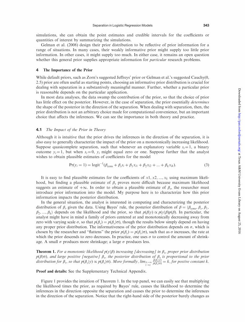
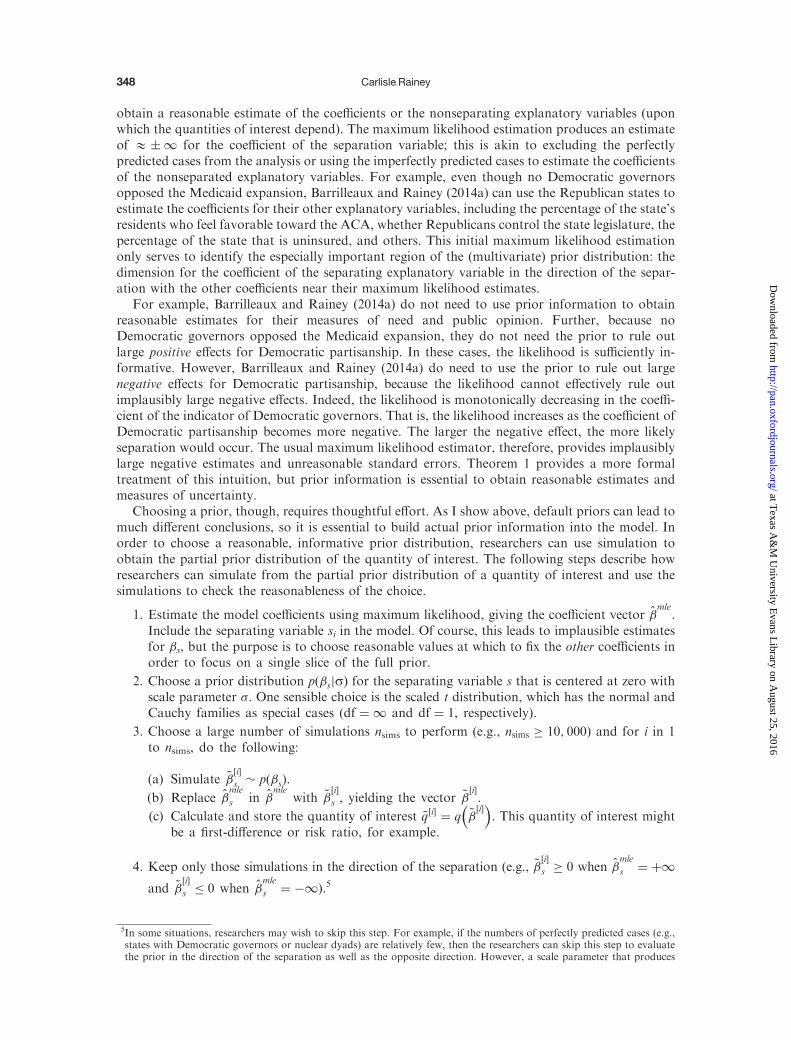
The first step in dealing with the separation in a principled manner is to choose a prior distributionthat represents actual prior information. To choose a reasonable prior, I follow the process aboveto generate a partial prior distribution for the risk ratio that Bell and Miller (2015) emphasize. Iexperimented with a range of prior distributions, from a variety of families, but settled on a normaldistribution with mean zero and standard deviation 4.5. This serves as an informative prior andrepresents my own prior beliefs. I chose this prior distribution because it essentially rules out riskratios larger than 1000—effects that I find implausibly large—and treats risk ratios smaller than1000 as plausible. Figure 4 and Table 1 summarize the partial prior distributions for this normaldistribution with standard deviation 4.5.

To evaluate the robustness of any statistical claims to the choice of prior, I also selected a highlyskeptical and highly enthusiastic prior. I chose a normal distribution with mean zero and standarddeviation 2 to serve as a skeptical prior that represents the belief that any pacifying effect of nuclearweapons is small (e.g., Mueller 1988). This skeptical prior distribution essentially rules out riskratios larger than 25 as implausibly large. Finally, I selected a normal distribution with mean zeroand standard deviation 8 to serve as an enthusiastic prior that represents the belief that the

Risk−Ratio (Log Scale)

0

200

400

600

800

1000

1200C

ount

s

Informative Normal(0, 4.5) Prior

1% ofsimulations

Risk−Ratio (Log Scale)

Skeptical Normal(0, 2) Prior

< 1% ofsimulations

Risk−Ratio (Log Scale)

Enthusiastic Normal(0, 8) Prior

14% ofsimulations

Fig. 4 This figure shows the partial prior distribution for the risk ratio of war in nonnuclear dyads tonuclear dyads. The risk ratio tells us how many times more likely war is in nonnuclear dyads compared to

nuclear dyads. Notice that the informative prior treats effects smaller than about 1000 as plausible, butessentially rules out larger effects. The skeptical prior essentially rules out effects larger than 25, whereas theenthusiastic prior treats effects between 1 and 100,000 as essentially equally likely.

6Bell and Miller (2015) also disagree with Rauchhaus’s (2009) coding of the 1999 conflict in Kargil between India andPakistan, which both possessed nuclear weapons. This conflict is excluded from Rauchhaus’s data set, but Bell andMiller argue that it should be included as a war between two nuclear-armed states, eliminating the problem ofseparation.

7Rauchhaus (2009) does not use a formal prior distribution, but uses generalized estimating equations, which we mightinterpret as having an improper, uniform prior on the logistic regression coefficients from minus infinity to plus infinity.The estimate is finite only due to a stopping rule in the iterative optimization algorithm.

Carlisle Rainey350

at Texas A

&M

University E

vans Library on A

ugust 25, 2016http://pan.oxfordjournals.org/

Dow

nloaded from

pacifying effects of nuclear weapons might be quite large (e.g., Mearsheimer 1993). This enthusi-astic prior, on the other hand, treats risk ratios as large as 500,000 as plausible. Figure 4 shows thepartial prior distributions for the informative, skeptical, and enthusiastic prior distributions. Forconvenience, Table 1 provides the deciles of the partial prior distributions shown in Fig. 4.

Notice that the skeptical prior suggests that risk ratios above and below 4 are equally likely (i.e.,50th percentile of the partial prior distribution is 3.9), whereas the enthusiastic prior suggests thateffects above and below 220 are equally likely. The informative prior, on the other hand, suggests(more reasonably, in my view) that the effect is equally likely to fall above and below 20. Thesethree prior distributions, along with the defaults suggested by Zorn (2005) and Gelman et al. (2008),provide a range of distributions to represent a range of prior beliefs.

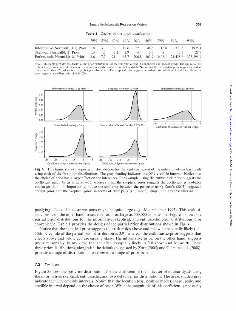
7.2 Posterior

Figure 5 shows the posterior distributions for the coefficient of the indicator of nuclear dyads usingthe informative, skeptical, enthusiastic, and two default prior distributions. The areas shaded grayindicate the 90% credible intervals. Notice that the location (e.g., peak or mode), shape, scale, andcredible interval depend on the choice of prior. While the magnitude of this coefficient is not easily

0.00

0.05

0.10

0.15

0.20

0.25

Pos

terio

r D

ensi

ty

Informative Normal(0, 4.5) Prior Skeptical Normal(0, 2) Prior Enthusiastic Normal(0, 8) Prior

−20 −15 −10 −5 0 5

Coefficient of Symmetric Nuclear Dyads

−20 −15 −10 −5 0 5

Coefficient of Symmetric Nuclear Dyads

0.00

0.05

0.10

0.15

0.20

0.25

Pos

terio

r D

ensi

ty

Zorn's Default Jeffreys' Prior

−20 −15 −10 −5 0 5

Coefficient of Symmetric Nuclear Dyads

Gelman et al.'s Default Cauchy(0, 2.5) Prior

Fig. 5 This figure shows the posterior distribution for the logit coefficient of the indicator of nuclear dyadsusing each of the five prior distributions. The gray shading indicates the 90% credible interval. Notice thatthe choice of prior has a large effect on the inferences. For example, using the enthusiastic prior suggests thecoefficient might be as large as �15, whereas using the skeptical prior suggests the coefficient is probably

not larger than �4. Importantly, notice the similarity between the posterior using Zorn’s (2005) suggesteddefault prior and the skeptical prior, in terms of their peak (i.e., mode), shape, and credible interval.

Table 1 Deciles of the prior distribution

10% 20% 30% 40% 50% 60% 70% 80% 90%

Informative Normal(0, 4.5) Prior 1.8 3.3 6 10.6 22 48.6 118.8 377.5 1975.1Skeptical Normal(0, 2) Prior 1.3 1.7 2.2 2.9 4 5.5 8 13.3 28.7Enthusiastic Normal(0, 8) Prior 2.6 7.7 21 63.7 206.8 803.9 3408.1 21,438.6 335,395.4

Notes: This table provides the deciles of the prior distribution for the risk ratio of war in nonnuclear and nuclear dyads. The risk ratio tellsus how many times more likely war is in nonnuclear dyads compared to nuclear dyads. Notice that the informative prior suggests a medianrisk ratio of about 20, which is a large, but plausible, effect. The skeptical prior suggests a median ratio of about 4 and the enthusiasticprior suggests a median ratio of over 200.

Separation in Logistic Regression Models 351

at Texas A

&M

University E

vans Library on A

ugust 25, 2016http://pan.oxfordjournals.org/

Dow

nloaded from

interpretable, notice that Gelman et al.’s (2008) suggested default prior is somewhat similar to theinformative prior, but Zorn’s (2005) suggested default is quite similar to the skeptical prior. Thus,these distributions illustrate that the prior is important when dealing with separation. Indeed, it is acritical step in obtaining reasonable inferences.

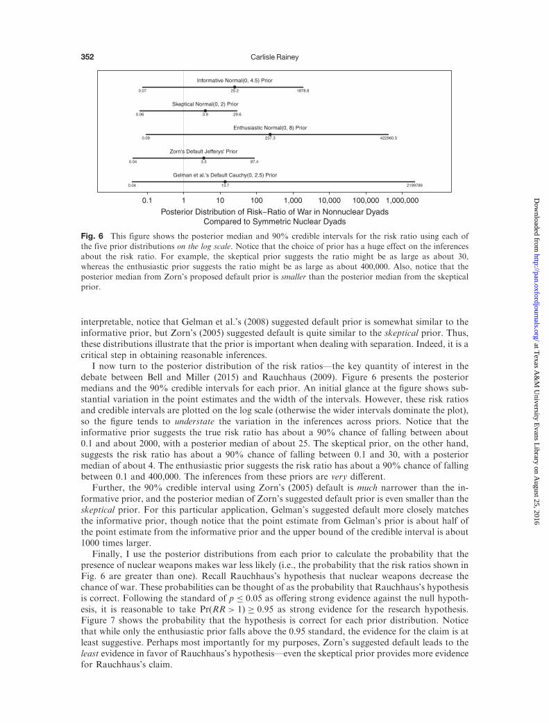
I now turn to the posterior distribution of the risk ratios—the key quantity of interest in thedebate between Bell and Miller (2015) and Rauchhaus (2009). Figure 6 presents the posteriormedians and the 90% credible intervals for each prior. An initial glance at the figure shows sub-stantial variation in the point estimates and the width of the intervals. However, these risk ratiosand credible intervals are plotted on the log scale (otherwise the wider intervals dominate the plot),so the figure tends to understate the variation in the inferences across priors. Notice that theinformative prior suggests the true risk ratio has about a 90% chance of falling between about0.1 and about 2000, with a posterior median of about 25. The skeptical prior, on the other hand,suggests the risk ratio has about a 90% chance of falling between 0.1 and 30, with a posteriormedian of about 4. The enthusiastic prior suggests the risk ratio has about a 90% chance of fallingbetween 0.1 and 400,000. The inferences from these priors are very different.

Further, the 90% credible interval using Zorn’s (2005) default is much narrower than the in-formative prior, and the posterior median of Zorn’s suggested default prior is even smaller than theskeptical prior. For this particular application, Gelman’s suggested default more closely matchesthe informative prior, though notice that the point estimate from Gelman’s prior is about half ofthe point estimate from the informative prior and the upper bound of the credible interval is about1000 times larger.

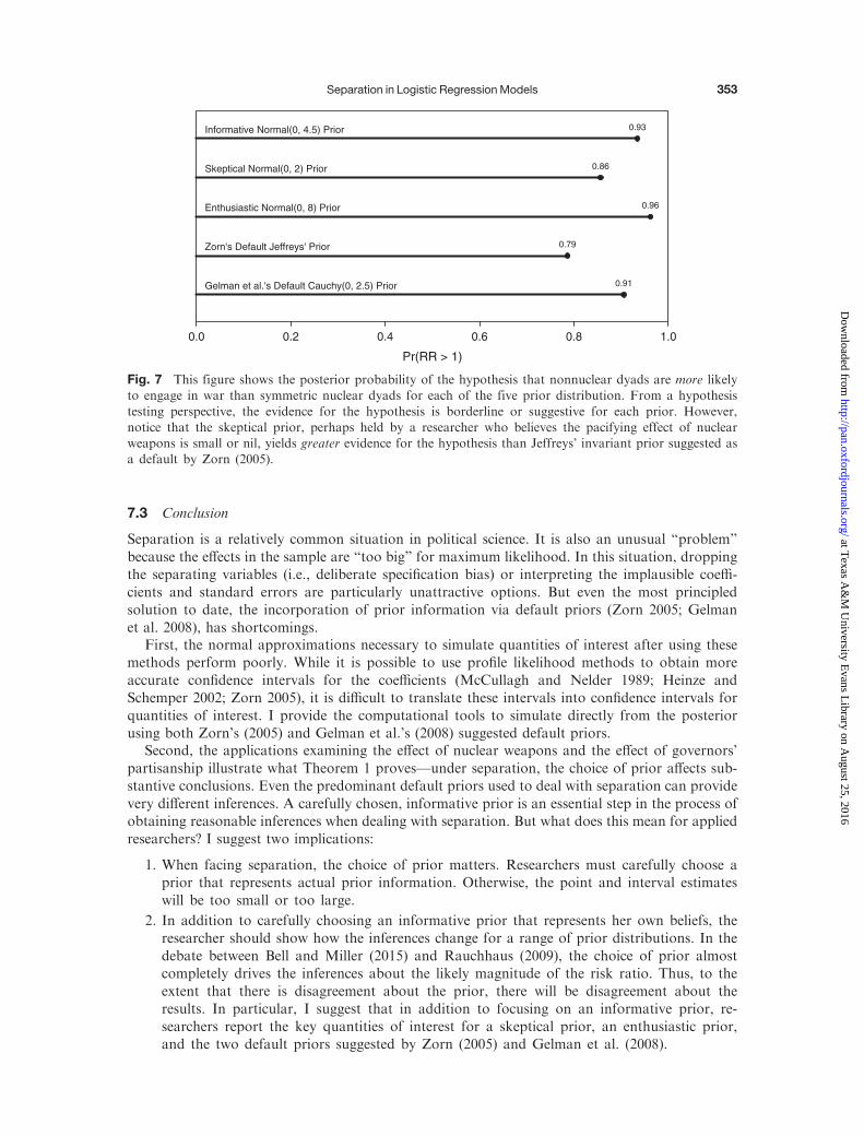
Finally, I use the posterior distributions from each prior to calculate the probability that thepresence of nuclear weapons makes war less likely (i.e., the probability that the risk ratios shown inFig. 6 are greater than one). Recall Rauchhaus’s hypothesis that nuclear weapons decrease thechance of war. These probabilities can be thought of as the probability that Rauchhaus’s hypothesisis correct. Following the standard of p � 0:05 as offering strong evidence against the null hypoth-esis, it is reasonable to take PrðRR > 1Þ � 0:95 as strong evidence for the research hypothesis.Figure 7 shows the probability that the hypothesis is correct for each prior distribution. Noticethat while only the enthusiastic prior falls above the 0.95 standard, the evidence for the claim is atleast suggestive. Perhaps most importantly for my purposes, Zorn’s suggested default leads to theleast evidence in favor of Rauchhaus’s hypothesis—even the skeptical prior provides more evidencefor Rauchhaus’s claim.

Fig. 6 This figure shows the posterior median and 90% credible intervals for the risk ratio using each of

the five prior distributions on the log scale. Notice that the choice of prior has a huge effect on the inferencesabout the risk ratio. For example, the skeptical prior suggests the ratio might be as large as about 30,whereas the enthusiastic prior suggests the ratio might be as large as about 400,000. Also, notice that the

posterior median from Zorn’s proposed default prior is smaller than the posterior median from the skepticalprior.

Carlisle Rainey352

at Texas A

&M

University E

vans Library on A

ugust 25, 2016http://pan.oxfordjournals.org/

Dow

nloaded from

7.3 Conclusion

Separation is a relatively common situation in political science. It is also an unusual “problem”

because the effects in the sample are “too big” for maximum likelihood. In this situation, droppingthe separating variables (i.e., deliberate specification bias) or interpreting the implausible coeffi-

cients and standard errors are particularly unattractive options. But even the most principledsolution to date, the incorporation of prior information via default priors (Zorn 2005; Gelman

et al. 2008), has shortcomings.First, the normal approximations necessary to simulate quantities of interest after using these

methods perform poorly. While it is possible to use profile likelihood methods to obtain more

accurate confidence intervals for the coefficients (McCullagh and Nelder 1989; Heinze andSchemper 2002; Zorn 2005), it is difficult to translate these intervals into confidence intervals for

quantities of interest. I provide the computational tools to simulate directly from the posteriorusing both Zorn’s (2005) and Gelman et al.’s (2008) suggested default priors.

Second, the applications examining the effect of nuclear weapons and the effect of governors’

partisanship illustrate what Theorem 1 proves—under separation, the choice of prior affects sub-stantive conclusions. Even the predominant default priors used to deal with separation can provide

very different inferences. A carefully chosen, informative prior is an essential step in the process ofobtaining reasonable inferences when dealing with separation. But what does this mean for applied

researchers? I suggest two implications:

1. When facing separation, the choice of prior matters. Researchers must carefully choose aprior that represents actual prior information. Otherwise, the point and interval estimates

will be too small or too large.

2. In addition to carefully choosing an informative prior that represents her own beliefs, theresearcher should show how the inferences change for a range of prior distributions. In the

debate between Bell and Miller (2015) and Rauchhaus (2009), the choice of prior almostcompletely drives the inferences about the likely magnitude of the risk ratio. Thus, to the

extent that there is disagreement about the prior, there will be disagreement about theresults. In particular, I suggest that in addition to focusing on an informative prior, re-

searchers report the key quantities of interest for a skeptical prior, an enthusiastic prior,and the two default priors suggested by Zorn (2005) and Gelman et al. (2008).

0.0 0.2 0.4 0.6 0.8 1.0

Pr(RR > 1)

Informative Normal(0, 4.5) Prior 0.93

Skeptical Normal(0, 2) Prior 0.86

Enthusiastic Normal(0, 8) Prior 0.96

Zorn's Default Jeffreys' Prior 0.79

Gelman et al.'s Default Cauchy(0, 2.5) Prior 0.91

Fig. 7 This figure shows the posterior probability of the hypothesis that nonnuclear dyads are more likelyto engage in war than symmetric nuclear dyads for each of the five prior distribution. From a hypothesis

testing perspective, the evidence for the hypothesis is borderline or suggestive for each prior. However,notice that the skeptical prior, perhaps held by a researcher who believes the pacifying effect of nuclearweapons is small or nil, yields greater evidence for the hypothesis than Jeffreys’ invariant prior suggested asa default by Zorn (2005).

Separation in Logistic Regression Models 353

at Texas A

&M

University E

vans Library on A

ugust 25, 2016http://pan.oxfordjournals.org/

Dow

nloaded from

When facing separation, researchers must carefully choose a prior distribution to nearly rule outimplausibly large effects. This article introduces the concept of a partial prior distribution and theassociated computational tools to help researchers choose a prior distribution that represents actualprior information for their particular research problem. By presenting results using several priordistributions, including an informative prior, researchers can increase the transparency, credibility,and accuracy of their inferences when dealing with separation.

References

Ahlquist, John S. 2010. Building strategic capacity: The political underpinning of coordinated wage bargaining. American

Political Science Review 104(1):171–88.

Albert, A., and J. A. Anderson. 1984. On the existence of maximum likelihood estimates in logistic regression models.

Biometrika 71(1):1–10.

Barrilleaux, Charles, and Carlisle Rainey. 2014a. The politics of need: Examining governors’ decisions to oppose the

“Obamacare” Medicaid expansion. State Politics and Policy Quarterly 14(4):437–60.

———. 2014b. Replication data for: The politics of need: Examining governors’ decisions to oppose the “Obamacare”

Medicaid expansion. http://dx.doi.org/10.15139/S3/12130.

Bell, Mark S., and Nicholas L. Miller. 2011. Replication data for: Questioning the stability-instability paradox. http://hdl.

handle.net/1902.1/15892.

———. 2015. Questioning the effect of nuclear weapons on conflict. Journal of Conflict Resolution 59(1):74–92.

Berry, Frances Stokes, and William D. Berry. 1990. State lottery adoptions as policy innovations: An event history

analysis. American Political Science Review 84(2):395–415.

Box, George E. P., and George C. Taio. 2011. Bayesian inference in statistical analysis. New York: John Wiley and Sons.

Brown, Robert L., and Jeffrey M. Kaplow. 2014. Talking peace: IAEA technical cooperation and nuclear proliferation.

Journal of Conflict Resolution 58(3):402–28.

Bueno de Mesquita, Bruce, and William Riker. 1982. An assessment of the merits of selective nuclear proliferation.

Journal of Conflict Resolution 26(2):283–306.

Carpenter, Bob, Andrew Gelman, Matt Hoffman, Daniel Lee, Ben Goodrich, Michael Betancourt, Michael A. Brubaker,

Jiqiang Guo, Peter Li, and Allen Riddell. 2016. Stan: A probabilistic programming language. Journal of Statistical

Software, forthcoming.

Casella, George, and Roger L. Berger. 2002. Statistical inference, 2nd ed. Pacific Grove, CA: Duxbury.

Casellas, Jason P. 2009. Coalitions in the House? The election of minorities to state legislatures and Congress. Political

Research Quarterly 62(1):120–31.

Cederman, Lars-Erik, Kristian Skrede Gleditsch, and Simon Hug. 2013. Elections and ethnic civil war. Comparative

Political Studies 46(3):387–417.

Cox, Gary W., Thad Kousser, and Matthew D. McCubbins. 2010. Party power or preferences? Quasi-experimental

evidence from American state legislatures. Journal of Politics 72(3):799–811.

DeRouen, Karl R. Jr., and Jacob Bercovitch. 2008. Enduring internal rivalries: A new framework for the study of civil

war. Journal of Peace Research 45(1):55–74.

Desposato, Scott, and Ethan Scheiner. 2008. Governmental centralization and party affiliation: Legislator strategies in

Brazil and Japan. American Political Science Review 102(4):509–24.

Fearon, James D. 1994. Signaling versus the balance of power and interests: An empirical test of a crisis bargaining

model. Journal of Conflict Resolution 38(2):236–69.

Firth, David. 1993. Bias reduction of maximum likelihood estimates. Biometrika 80(1):27–38.

Fuhrmann, Matthew. 2012. How “Atoms for Peace” programs cause nuclear insecurity. Ithica, NY: Cornell University

Press.

Gelman, Andrew. 2008. Scaling regression inputs by dividing by two standard deviations. Statistics in Medicine

27(15):2865–73.

Gelman, Andrew, and Aleks Jakulin. 2007. Bayes: Radical, liberal, or conservative? Statistica Sinica 17(2):422–26.

Gelman, Andrew, Aleks Jakulin, Maria Grazia Pittau, and Yu-Sung Su. 2008. A weakly informative prior distribution for

logistic and other regression models. Annals of Applied Statistics 2(4):1360–83.

Geyer, Charles J. 2009. Likelihood inference in exponential families and directions of recession. Electronic Journal of

Statistics 3:259–89.

Gill, Jeff. 2008. Bayesian methods: A social and behavioral science approach, 2nd ed. Boca Raton, FL: Chapman and Hall.

Gill, Jeff, and Lee D. Walker. 2005. Elicited priors for Bayesian model specifications in political science research. Journal

of Politics 67(3):841–72.

Gross, Justin H. 2015. Testing what matters (if you must test at all): A context-driven approach to substantive and

statistical significance. American Journal of Political Science 59(3):775–788.

Heinze, Georg, and Michael Schemper. 2002. A solution to the problem of separation in logistic regression. Statistics in

Medicine 21(16):2409–19.

Heller, William B., and Carol Mershon. 2008. Dealing in discipline: Party switching and legislative voting in the Italian

Chamber of Deputies, 1988–2000. American Journal of Political Science 52(4):910–24.

Carlisle Rainey354

at Texas A

&M

University E

vans Library on A

ugust 25, 2016http://pan.oxfordjournals.org/

Dow

nloaded from

Jackman, Simon. 2000. Estimation and inference via Bayesian simulation: An introduction to Markov chain Monte

Carlo. American Journal of Political Science 44(2):369–98.

Jeffreys, H. 1946. An invariant form of the prior probability in estimation problems. Proceedings of the Royal Society of

London A 186(1007):453–61.

King, Gary, Michael Tomz, and Jason Wittenberg. 2000. Making the most of statistical analyses: Improving interpret-

ation and presentation. American Journal of Political Science 44(2):341–55.

Leeman, Lucas, and Isabella Mares. 2014. The adoption of proportional representation. Journal of Politics 76(2):461–78.

Lesaffre, E., and A. Albert. 1989. Partial separation in logistic discrimination. Journal of the Royal Statistical Society B

51(1):109–16.

Mares, Isabela. 2015. From open secrets to secret voting: Democratic electoral reforms and voter autonomy. Cambridge

Studies in Comparative Politics. Cambridge, UK: Cambridge University Press.

Martin, Lanny W., and Randolph T. Stevenson. 2001. Government formation in parliamentary democracies. American

Journal of Political Science 45(1):33–50.

McCullagh, Peter, and John A. Nelder. 1989. Generalized linear models, 2nd ed. Boca Raton, FL: Chapman and Hall.

Mearsheimer, John J. 1993. The case for a Ukrainian nuclear deterrent. Foreign Affairs 72(3):50–66.

Minozzi, William, and Craig Volden. 2013. Who heeds the call of the party in Congress? Journal of Politics 75(3):787–802.

Mueller, John. 1988. The essential irrelevance of nuclear weapons: Stability in the postwar world. International Security

13(2):55–79.

Peterson, Timothy M., and A. Cooper Drury. 2011. Sanctioning violence: The effect of third-party economic coercion on

militarized conflict. Journal of Conflict Resolution 55(4):580–605.

Poirier, Dale. 1994. Jeffreys’ prior for logit models. Journal of Econometrics 63(2):327–39.

Rainey, Carlisle. 2014. Arguing for a negligible effect. American Journal of Political Science 58(4):1083–91.

———. 2016. Replication data for: Dealing with separation in logistic regression models. http://dx.doi.org/10.7910/DVN/

VW7G2Q.

Rauchhaus, Robert. 2009. Evaluating the nuclear peace hypothesis: A quantitative approach. Journal of Conflict

Resolution 53(2):258–78.

Reiter, Dan. 2014. Security commitments and nuclear proliferation. Foreign Policy Analysis 10(1):61–80.

Rocca, Michael S., Gabriel R. Sanchez, and Jason L. Morin. 2011. The institutional mobility of minority members of

Congress. Political Research Quarterly 64(4):897–909.

Sagan, Scott D. 1994. The perils of proliferation. International Security 18(4):66–107.

Smith, Daniel A., and Dustin Fridkin. 2008. Delegating direct democracy: Interparty legislative competition and the

adoption of the initiative in the American states. American Political Science Review 102(3):333–350.

Stan Development Team. 2016a. RStan: The R interface to Stan, Version 2.9.0. http://mc-stan.org.

———. 2016b. RStanArm: Bayesian applied regression modeling via Stan. http://mc-stan.org.

Vining, Richard L. Jr., Teena Wilhelm, and Jack D. Collens. 2015. A market-based model of state Supreme Court news:

Lessons from capital cases. State Politics and Policy Quarterly 15(1):3–23.

Weisiger, Alex. 2014. Victory without peace: Conquest, insurgency, and war termination. Conflict Management and Peace

Science 31(4):357–82.

Western, Bruce, and Simon Jackman. 1994. Bayesian inference for comparative research. American Political Science

Review 88(2):412–23.

Wolfinger, Raymond E., and Steven J. Rosenstone. 1980. Who votes? New Haven: Yale University Press.

Zorn, Christopher. 2005. A solution to separation in binary response models. Political Analysis 13(2):157–70.

Separation in Logistic Regression Models 355

at Texas A

&M

University E

vans Library on A

ugust 25, 2016http://pan.oxfordjournals.org/

Dow

nloaded from