Dealing with Structural Breaks∗

Pierre Perron

Boston University

This version: April 20, 2005

Abstract

This chapter is concerned with methodological issues related to estimation, testingand computation in the context of structural changes in the linear models. A centraltheme of the review is the interplay between structural change and unit root and onmethods to distinguish between the two. The topics covered are: methods relatedto estimation and inference about break dates for single equations with or withoutrestrictions, with extensions to multi-equations systems where allowance is also madefor changes in the variability of the shocks; tests for structural changes including testsfor a single or multiple changes and tests valid with unit root or trending regressors,and tests for changes in the trend function of a series that can be integrated or trend-stationary; testing for a unit root versus trend-stationarity in the presence of structuralchanges in the trend function; testing for cointegration in the presence of structuralchanges; and issues related to long memory and level shifts. Our focus is on theconceptual issues about the frameworks adopted and the assumptions imposed as theyrelate to potential applicability. We also highlight the potential problems that canoccur with methods that are commonly used and recent work that has been done toovercome them.

∗This paper was prepared for the Palgrave Handbook of Econometrics, Vol. 1: Econometric Theory.For useful comments on an earlier draft, I wish to thank Jushan Bai, Songjun Chun, Ai Deng, MohitoshKejriwal, Dukpa Kim, Eiji Kurozumi, Zhongjun Qu, Jonathan Treussard, Tim Vogelsang, Tatsuma Wada,Tomoyoshi Yabu, Yunpeng Zhang, Jing Zhou.

1 Introduction

This chapter is concerned with methodological issues related to estimation, testing and

computation for models involving structural changes. The amount of work on this subject

over the last 50 years is truly voluminous in both the statistics and econometrics literature.

Accordingly, any survey article is bound by the need to focus on specific aspects. Our aim

is to review developments in the last fifteen years as they relate to econometric applications

based on linear models, with appropriate mention of prior work to better understand the

historical context and important antecedents. During this recent period, substantial advances

have been made to cover models at a level of generality that allows a host of interesting

practical applications. These include models with general stationary regressors and errors

that can exhibit temporal dependence and heteroskedasticity, models with trending variables

and possible unit roots, cointegrated models and long memory processes, among others.

Advances in these contexts have been made pertaining to the following topics: computational

aspects of constructing estimates, their limit distributions, tests for structural changes, and

methods to determine the number of changes present.

These recent developments related to structural changes have paralleled developments

in the analysis of unit root models. One reason is that many of the tools used are similar.

In particular, heavy use is made in both literatures of functional central limit theorems or

invariance principles, which have fruitfully been used in many areas of econometrics. At the

same time, a large literature has addressed the interplay between structural changes and

unit roots, in particular the fact that both classes of processes contain similar qualitative

features. For example, most tests that attempt to distinguish between a unit root and a

(trend) stationary process will favor the unit root model when the true process is subject to

structural changes but is otherwise (trend) stationary within regimes specified by the break

dates. Also, most tests trying to assess whether structural change is present will reject the

null hypothesis of no structural change when the process has a unit root component but

with constant model parameters. As we can see, there is an intricate interplay between unit

root and structural changes. This creates particular difficulties in applied work, since both

are of definite practical importance in economic applications. A central theme of this review

relates to this interplay and to methods to distinguish between the two.

The topics addressed in this review are the following. Section 2 provides interesting

historical notes on structural change, unit root and long memory tests which illustrate the

intricate interplay involved when trying to distinguish between these three features. Section

1

3 reviews methods related to estimation and inference about break dates. We start with

a general linear regression model that allows multiple structural changes in a subset of the

coefficients (a partial change model) with the estimates obtained by minimizing the sum of

squared residuals. Special attention is given to the set of assumptions used to obtain the

relevant results and their relevance for practical applications (Section 3.1). We also include a

discussion of results applicable when linear restrictions are imposed (3.2), methods to obtain

estimates of the break dates that correspond to global minimizers of the objective function

(3.3), the limit distributions of such estimates, including a discussion of benefits and poten-

tial drawbacks that arise from the adoption of a special asymptotic framework that considers

shifts of shrinking magnitudes (3.4). Section 3.5 briefly discusses an alternative estimation

strategy based on estimating the break dates sequentially, and Section 3.6 discusses exten-

sions of most of these issues to a general multi-equations system, which also allows changes

in the covariance matrix of the errors.

Section 4 considers tests for structural changes. We start in Section 4.1 with meth-

ods based on scaled functions of partial sums of appropriate residuals. The CUSUM test

is probably the best known example but the class includes basically all methods available

for general models prior to the early nineties. Despite their wide appeal, these tests suffer

from an important drawback, namely that power is non-monotonic, in the sense that the

power can decrease and even go to zero as the magnitude of the change increases (4.2).

Section 4.3 discusses tests that directly allow for a single break in the regression underlying

their construction, including a class of optimal tests that have found wide appeal in prac-

tice (4.3.1), but which are also subject to non-monotonic power when two changes affect

the system (4.3.2), a result which points to the usefulness of tests for multiple structural

changes discussed in Section 4.4. Tests for structural changes in the linear model subject to

restrictions on the parameters are discussed in Section 4.5 and extensions of the methods

to multivariate systems are presented in Section 4.6. Tests valid when the regressors are

unit root processes and the errors are stationary, i.e., cointegrated systems, are reviewed in

Section 4.7, while Section 4.8 considers recent developments with respect to tests for changes

in a trend function when the noise component of the series is either a stationary or a unit

root process.

Section 5 addresses the topic of testing for a unit root versus trend-stationarity in the

presence of structural changes in the trend function. The motivation, issues and frameworks

are presented in Section 5.1, while Section 5.2 discusses results related to the effect of changes

in the trend on standard unit root tests. Methods to test for a unit root allowing for a change

2

at a known date are reviewed in Section 5.3, while Section 5.4 considers the case of breaks

occurring at unknown dates including problems with commonly used methods and recent

proposals to overcome them (Section 5.4.2).

Section 6 tackles the problem of testing for cointegration in the presence of structural

changes in the constant and/or the cointegrating vector. We review first single equation

methods (Section 6.1) and then, in Section 6.2, methods based on multi-equations systems

where the object of interest is to determine the number of cointegrating vectors. Finally,

Section 7 presents concluding remarks outlining a few important topics for future research

and briefly reviews similar issues that arise in the context of long memory processes, an

area where issues of structural changes (in particular level shifts) have played an important

role recently, especially in light of the characterization of the time series properties of stock

return volatility.

Our focus is on conceptual issues about the frameworks adopted and the assumptions

imposed as they relate to potential applicability. We also highlight problems that can occur

with methods that are commonly used and recent work that has been done to overcome

them. Space constraints are such that a detailed elicitation of all procedures discussed is

not possible and the reader should consult the original work for details needed to implement

them in practice.

Even with a rich agenda, this review inevitably has to leave out a wide range of important

work. The choice of topic is clearly closely related to the author’s own past and current work,

and it is, accordingly, not an unbiased review, though we hope that a balanced treatment

has been achieved to provide a comprehensive picture of how to deal with breaks in linear

models.

Important parts of the literature on structural change that are not covered include,

among others, the following: methods related to the so-called on-line approach where the

issue is to detect whether a change sas occurred in real time; results pertaining to non-linear

models, in particular to tests for structural changes in a Generalized Method of Moment

framework; smooth transition changes and threshold models; non parametric methods to

estimate and detect changes; Bayesian methods; issues related to forecasting in the presence

of structural changes; theoretical results and methods related to specialized cases that are

not of general interest in economics; structural change in seasonal models; and bootstrap

methods. The reader interested in further historical developments and methods not covered

in this survey can consult the books by Clements and Hendry (1999), Csörgo and Horváth

(1997), Krämer and Sonnberger (1986), Hackl and Westlund (1991), Hall (2005), Hatanaka

3

and Yamada (2003), Maddala nd Kim (1998), Tong (1990) and the following review articles:

Bhattacharya (1994), Deshayes and Picard (1986), Hackl and Westlund (1989), Krishnaiah

and Miao (1988), Perron (1994), Pesaran et al. (1985), Shaban (1980), Stock (1994), van

Dijk et al. (2002) and Zacks (1983).

2 Introductory Historical Notes

It will be instructive to start with some interesting historical notes concerning early tests

for structural change. Consider a univariate time series, yt; t = 1, ..., T, which under thenull hypothesis is independently and identically distributed with mean µ and finite variance.

Under the alternative hypothesis, yt is subject to a one time change in mean at some unknown

date Tb, i.e.,

yt = µ1 + µ21(t > Tb) + et (1)

where et ∼ i.i.d. (0, σ2e) and 1(·) denotes the indicator function. Quandt (1958, 1960) hadintroduced what is now known as the Sup F test (assuming normally distributed errors), i.e.,

the likelihood ratio test for a change in parameters evaluated at the break date that maxi-

mizes the likelihood function. However, the limit distribution was then unknown. Quandt

(1960) had shown that it was far from being a chi-square distribution and resorted to tab-

ulate finite sample critical values for selected cases. Following earlier work by Chernoff

and Zacks (1964) and Kander and Zacks (1966), an alternative approach was advocated by

Gardner (1969) steemming from a suggestion by Page (1955, 1957) to use partial sums of

demeaned data to analyze structural changes (see more on this below). The test considered

is Bayesian in nature and, under the alternative, assigns weights pt as the prior probability

that a change occurs at date t (t = 1, ..., T ). Assuming Normal errors and an unknown value

of σ2e, this strategy leads to the test

Q = σ−2e T−1TXt=1

pt

"TX

j=t+1

(yj − y)

#2where y = T−1

PTt=1 yt, is the sample average, and σ2e = T−1

PTt=1(yt − y)2 is the sample

variance of the data. With a prior that assigns equal weight to all observations, i.e. pt = 1/T ,

the test reduces to

Q = σ−2e T−2TXt=1

"TX

j=t+1

(yj − y)

#2Under the null hypothesis, the test can be expressed as a ratio of quadratic forms in Normal

variates and standard numerical method can be used to evaluate its distribution (e.g., Imhof,

4

1961, though Gardner originally analyzed the case with σ2e known). The limit distribution

of the statistic Q was analyzed by MacNeill (1974). He showed that

Q⇒Z 1

0

B0(r)2dr

where B0(r) = W (r) − rW (1) is a Brownian bridge, and noted that percentage point had

already been derived by Anderson and Darling (1952) in the context of goodness of fit tests.

MacNeill (1978) extended the procedure to test for a change in a polynomial trend function

of the form

yt =

pXi=0

βi,tti + et

where

βi,t = βi + δi1(t > Tb)

The test of no change (δi = 0 for all i) is then

Qp = σ−2e T−2TXt=1

"TX

j=t+1

ej

#2

with σ2e = T−1PT

t=1 e2t and et the residuals from a regression of yt on 1, t, ..., tp. The limit

distribution is given by

Q⇒Z 1

0

Bp(r)2dr

where Bp(r) is a generalized Brownian bridge. MacNeill (1978) computed the critical values

by exact numerical methods up to six decimals accuracy (showing, for p = 0, the critical

values of Anderson and Darling (1952) to be very accurate). The test was extended to

allow dependence in the errors et by Perron (1991) and Tang and MacNeill (1993) (see

also Kulperger, 1987a,b, Jandhyala and MacNeill, 1989, Jandhyala and Minogue, 1993, and

Antoch et al., 1997). In particular, Perron (1991) shows that, under general conditions, the

same limit distribution obtains using the statistic

Q∗p = he(0)−1T−2

TXt=1

"TX

j=t+1

ej

#2

where he(0) is a consistent estimate of (2π times) the spectral density function at frequency

zero of et.

5

Even though, little of this filtered through the econometrics literature, the statistic Q∗p is

well known to applied economists. It is the so-called KPSS test for testing the null hypothesis

of stationarity versus the alternative of a unit root, see Kwiatkowski et al. (1992). More

precisely, Qp is the Lagrange Multiplier (LM) and locally best invariant (LBI) test for testing

the null hypothesis that σ2u = 0 in the model

yt =

pXi=0

βi,tti + rt + et

rt = rt−1 + ut

with ut ∼ i.i.d. N(0, σ2u) and et ∼ i.i.d. N(0, σ2e). Q∗p is then the corresponding large sample

counterpart that allows correlation. Kwiatkowski et al. (1992) provided critical values for

p = 0 and 1 using simulations (which are less precise than the critical values of Anderson

and Darling, 1952, and MacNeill, 1978). In the econometrics literature, several extensions

of this test have been proposed; in particular for testing the null hypothesis of cointegration

versus the alternative of no cointegration (Nyblom and Harvey, 2000) and testing whether

any part of a sample shows a vector of series to be cointegrated (Qu, 2004). Note also that

the same test can be given the interpretation of a LBI for parameter constancy versus the

alternative that the parameters follow a random walk (e.g., Nyblom and Mäkeläinen, 1983,

Nyblom, 1989, Nabeya and Tanaka, 1988, Jandhyala and MacNeill, 1992, Hansen, 1992b).

The same statistic is also the basis for a test of the null hypothesis of no-cointegration when

considering functional of its reciprocal (Breitung, 2002).

So what are we to make of all of this? The important message to learn from the fact that

the same statistic can be applied to tests for stationarity versus either unit root or structural

change is that the two issues are linked in important ways. Evidence in favor of unit roots

can be a manifestation of structural changes and vice versa. This was indeed an important

message of Perron (1989, 1990); see also Rappoport and Reichlin (1989). In this survey, we

shall return to this problem and see how it introduces severe complications when dealing

with structural changes and unit roots.

It is also of interest to go back to the work by Page (1955, 1957) who had proposed to

use partial sums of demeaned data to test for structural change. Let Sr =Pr

j=1(yj− y), his

procedure for a two-sided test for change in the mean is based on the following quantities

max0≤r≤T

∙Sr − min

0≤i<rSi

¸and max

0≤r≤T

∙min0≤i<r

Si − Sr

¸and looks whether either exceeds a threshold (which, in the symmetric case, is the same).

So we reject the null hypothesis if the partial sum rises enough from its previous minimum

6

or falls enough from its previous maximum. Nadler and Robbins (1971) showed that this

procedure is equivalent to looking at the statistic

RS =

∙max0≤r≤T

Sr − min0≤r≤T

Sr

¸i.e., to assess whether the range of the sequence of partial sums is large enough. But this is

also exactly the basis of the popular rescaled range procedure used to test the null hypothesis

of short-memory versus the alternative of long memory (see, in particular, Hurst, 1951,

Mandelbrot and Taqqu, 1979, Bhattacharya et al., 1983, and Lo, 1991).

This is symptomatic of the same problem discussed above from a slightly different angle;

structural change and long memory imply similar features in the data and, accordingly,

are hard to distinguish. In particular, evidence for long memory can be caused by the

presence of structural changes, and vice versa. The intuition is basically the same as the

message in Perron (1990), i.e., level shifts induce persistent features in the data. This

problem has recently received a lot of attention, especially in the finance literature concerning

the characteristics of stock returns volatility (see, in particular, Diebold and Inoue, 2001,

Gourieroux and Jasiak, 2001, Granger and Hyung, 2004, Lobato and Savin, 1998, and Perron

and Qu, 2004).

3 Estimation and Inference about Break Dates

In this section we discuss issues related to estimation and inference about the break dates in

a linear regression framework. The emphasis is on describing methods that are most useful

in applied econometrics, explaining the relevance of the conditions imposed and sketching

some important theoretical steps that help to understand particular assumptions made.

Following Bai (1997a) and Bai and Perron (1998), the main framework of analysis can

be described by the following multiple linear regression with m breaks (or m+ 1 regimes):

yt = x0tβ + z0tδj + ut, t = Tj−1 + 1, ..., Tj, (2)

for j = 1, ...,m + 1. In this model, yt is the observed dependent variable at time t; both

xt (p × 1) and zt (q × 1) are vectors of covariates and β and δj (j = 1, ...,m + 1) are the

corresponding vectors of coefficients; ut is the disturbance at time t. The indices (T1, ..., Tm),

or the break points, are explicitly treated as unknown (the convention that T0 = 0 and

Tm+1 = T is used). The purpose is to estimate the unknown regression coefficients together

with the break points when T observations on (yt, xt, zt) are available. This is a partial

7

structural change model since the parameter vector β is not subject to shifts and is estimated

using the entire sample. When p = 0, we obtain a pure structural change model where all

the model’s coefficients are subject to change. Note that using a partial structural change

models where only some coefficients are allowed to change can be beneficial both in terms

of obtaining more precise estimates and also in having can be more powerful tests.

The multiple linear regression system (2) may be expressed in matrix form as

Y = Xβ + Zδ + U,

where Y = (y1, ..., yT )0, X = (x1, ..., xT )

0, U = (u1, ..., uT )0, δ = (δ01, δ

02, ..., δ

0m+1)

0, and Z is

the matrix which diagonally partitions Z at (T1, ..., Tm), i.e. Z = diag(Z1, ..., Zm+1) with

Zi = (zTi−1+1, ..., zTi)0. We denote the true value of a parameter with a 0 superscript. In

particular, δ0 = (δ001 , ..., δ

00m+1)

0 and (T 01 , ..., T0m) are used to denote, respectively, the true

values of the parameters δ and the true break points. The matrix Z0 is the one which

diagonally partitions Z at (T 01 , ..., T0m). Hence, the data-generating process is assumed to be

Y = Xβ0 + Z0δ0 + U. (3)

The method of estimation considered is based on the least-squares principle. For each m-

partition (T1, ..., Tm), the associated least-squares estimates of β and δj are obtained by

minimizing the sum of squared residuals

(Y −Xβ − Zδ)0(Y −Xβ − Zδ) =m+1Xi=1

TiXt=Ti−1+1

[yt − x0tβ − z0tδi]2.

Let β(Tj) and δ(Tj) denote the estimates based on the given m-partition (T1, ..., Tm)

denoted Tj. Substituting these in the objective function and denoting the resulting sumof squared residuals as ST (T1, ..., Tm), the estimated break points (T1, ..., Tm) are such that

(T1, ..., Tm) = argmin(T1,...,Tm)ST (T1, ..., Tm), (4)

where the minimization is taken over some set of admissible partitions (see below). Thus

the break-point estimators are global minimizers of the objective function. The regres-

sion parameter estimates are the estimates associated with the m-partition Tj, i.e. β =

β(Tj), δ = δ(Tj).This framework includes many contributions made in the literature as special cases de-

pending on the assumptions imposed; e.g., single change, changes in the mean of a stationary

8

process, etc. However, the fact that the method of estimation is based on the least-squares

principle implies that, even if changes in the variance of ut are allowed, provided they occur

at the same dates as the breaks in the parameters of the regression, such changes are not

exploited to increase the precision of the break date estimators. This is due to the fact that

the least-squares method imposes equal weights on all residuals. Allowing different weights,

as needed when accounting for changes in variance, requires adopting a quasi-likelihood

framework, see below.

3.1 The assumptions and their relevance

To obtain theoretical results about the consistency and limit distribution of the break dates,

some conditions need to be imposed on the regressors, the errors, the set of admissible

partitions and the break dates. To our knowledge, the most general set of assumptions,

as far as applications are concerned, are those in Perron and Qu (2005). Some are simply

technical (e.g., invertibility requirements), while others restrict the potential applicability of

the results. Hence, it is useful to discuss the latter.

• Assumption on the regressors: Letwt = (x0t, z

0t)0, for i = 0, ...,m, (1/li)

PT 0i +[liv]

t=T0i +1wtw

0t →p

Qi(v) a non-random positive definite matrix uniformly in v ∈ [0, 1].

This assumption allows the distribution of the regressors to vary across regimes. It,

however, requires the data to be weakly stationary stochastic processes. It can, however,

be relaxed substantially, though the technical proofs then depend on the nature of the

relaxation. For instance the scaling used forbids trending regressors, unless they are of the

form 1, (t/T ), ..., (t/T )p, say, for a polynomial trend of order p. Casting trend functionsin this form can deliver useful results in many cases. However, there are instances where

specifying trends in unscaled form, i.e., 1, t, ..., tp, can deliver much better results, especiallyif level and trend slope changes occur jointly. Results using unscaled trends with p = 1

are presented in Perron and Zhu (2005). A comparison of their results with other trend

specifications is presented in Deng and Perron (2005).

Another important restriction is implied by the requirement that the limit be a fixed

matrix, as opposed to permitting it to be stochastic. This, along with the scaling, precludes

integrated processes as regressors (i.e., unit roots). In the single break case, this has been

relaxed by Bai, Lumsdaine and Stock (1998) who considered, among other things, structural

changes in cointegrated relationships. Consistency still applies but the rate of convergence

and limit distributions of the estimates are different. Another context in which integrated

9

regressors play a role is the case of changes in persistence. Chong (2001) considered an AR(1)

model where the autoregressive coefficient takes a value less than one before some break date

and value one after, or vice versa. He showed consistency of the estimate of the break date

and derived the limit distribution. When the move is from stationarity to unit root, the

rate of convergence is the same as in the stationary case (though the limit distribution is

different), but interestingly, the rate of convergence is faster when the change is from a unit

root to a stationary process. No results are yet available for multiple structural changes in

regressions involving integrated regressors, though work is in progress on this issue. The

problem here is more challenging because the presence of regressors with a unit root, whose

coeffients are subject to change, implies break date estimates with limit distributions that

are not independent, hence all break dates need to be evaluated jointly.

The sequence wtut satisfies the following set of conditions.

• Assumptions on the errors: Let the Lr-norm of a random matrix X be defined by

kXkr = (P

i

Pj E |Xij|r)1/r for r ≥ 1. (Note that kXk is the usual matrix norm or the

Euclidean norm of a vector.) With Fi : i = 1, 2, .. a sequence of increasing σ-fields,it is assumed that wiui,Fi forms a Lr-mixingale sequence with r = 2 + δ for some

δ > 0. That is, there exist nonnegative constants ci : i ≥ 1 and ψj : j ≥ 0 suchthat ψj ↓ 0 as j → ∞ and for all i ≥ 1 and j ≥ 0, we have: (a) kE(wiui|Fi−j)kr ≤ciψj, (b) kwiui −E(wiui|Fi+j)kr ≤ ciψj+1. Also assume (c) maxi ci ≤ K < ∞, (d)P∞

j=0 j1+kψj <∞, (e) kzik2r < M <∞ and kuik2r < N <∞ for some K,M,N > 0.

This imposes mild restrictions on the vector wtut and permits a wide class of poten-

tial correlation and heterogeneity (including conditional heteroskedasticity) and also allows

lagged dependent variables. It rules out errors that have unit roots. In this latter case, if

the regressors are stationary (or satisfy the Assumption on the regressors stated above), the

estimates of the break dates are inconsistent (see Nunes et al., 1995). However, unit root

errors can be of interest; for example when testing for a change in the deterministic compo-

nent of the trend function for an integrated series, in which case the estimates are consistent

(see Perron and Zhu, 2005). The set of conditions listed above are not the weakest possible.

For example, Lavielle and Moulines (2000) allow the errors to be strongly dependent, i.e.,

long memory processes such as fractionally integrated ones are permitted. They, however,

consider only the case of multiple changes in the mean. Technically, what is important is

to be able to establish a generalized Hájek-Rényi (1955) type inequality for the zero mean

variables ztut, as well as a Functional Central Limit Theorem and a Law of Large Numbers.

10

• Assumption on the minimization problem: The minimization problem defined by (4)

is taken over all possible partitions such that Ti − Ti−1 ≥ T for some > 0.

This requirement was introduced in Bai and Perron (1998) only for the case where lagged

dependent variables were allowed. When serial correlation in the errors was allowed they

introduced the requirement that the errors be independent of the regressors at all leads and

lags. This is obviously a strong assumption which is often violated in practice. The assump-

tion on the errors listed above are much weaker, in particular concerning the relation between

the errors and regressors. This weakening comes at the cost of a mild strengthening on the

assumption about the regressors and the introduction of the restriction on the minimization

problem. Note that the latter is also imposed in Lavielle and Moulines (2000), though they

note that it can be relaxed with stronger conditions on ztut or by constraining the estimates

to lie in a compact set.

• Assumption on the break dates: T 0i = [Tλ0i ] , where 0 < λ01 < ... < λ0m < 1.

This assumption specifies that the break dates are asymptotically distinct. While it is

standard, it is surprisingly the most controversial for some. The reason is that it dictates the

asymptotic framework adopted. With this condition, when the sample size T increases, all

segments increase in length in the same proportions to each other. Oftentimes, an asymptotic

analysis is viewed as a thought experiment about what would happen if we were able to collect

more and more data in the future. If one adheres to this view, then the last regime should

increase in length (assuming no other break will occur in the future) and all other segments

then become a negligible proportion of the total sample. Hence, as T increases, we would find

ourselves with a single segment, in which case the framework becomes useless. The fact is

that any asymptotic analysis is simply a device to enable us to get useful information about

the structure, which can help us understand the finite sample distributions, and hopefully

to deliver good approximations. The adoption of any asymptotic framework should only be

evaluated on this basis, no matter how ad hoc it may seem at first sight. Here, with say a

sample of size 100 and 3 breaks occurring at dates 25, 50 and 75, all segments are a fourth

of the total sample. It therefore makes sense to use an asymptotic framework whereby this

feature is preserved. The same comments apply to contexts in which some parameters are

made local to some boundary as the sample size increases. No claim whatsoever is made that

the parameter would actually change if more data were collected, yet such a device has been

found to be of great use and to provide very useful approximations. This applies to local

11

asymptotic power function, roots local to unity or shrinking size of shifts as we will discuss

later. Having said that, it does not mean that the asymptotic framework that is adopted

in this literature is the only one useful or even the best. For example, it is conceivable that

an asymptotic theory whereby more and more data are added keeping a fixed span of data

would be useful as well. However, such a continuous time limit distribution has not yet

appeared in the structural change context.

Under these conditions, the main theoretical results are that the break fractions λ0i are

consistently estimated, i.e., λi ≡ (Ti/T )→p λ0i and that the rate of convergence is T . More

precisely, for every ε > 0, there exists a C <∞, such that for large T ,

P (|T (λi − λ0i )| > C∆−2i ) < ε (5)

for every i = 1, ...,m, where ∆i = δi+1 − δi. Note that the estimates of the break dates

are not consistent themselves, but the differences between the estimates and the true values

are bounded by some constant, in probability. Also, this implies that the estimates of the

other parameters have the same distribution as would prevail if the break dates were known.

Kurozumi and Arai (2004) obtain a similar result with I(1) regressors for a cointegrated

model subject to a change in some parameters of the cointegrating vector. They show the

estimate of the break fraction obtained by minimizing the sum of squared residuals from the

static regression to converge at a fast enough rate for the estimates of the parameters of the

model to asymptotically unaffected by the estimation of the break date.

3.2 Allowing for restrictions on the parameters

Perron and Qu (2005) approach the issues of multiple structural changes in a broader frame-

work whereby arbitrary linear restrictions on the parameters of the conditional mean can be

imposed in the estimation. The class of models considered is

y = Zδ + u

where

Rδ = r

with R a k by (m+1)q matrix with rank k and r, a k dimensional vector of constants. The

assumptions are the same as discussed above. Note first that there is no need for a distinction

between variables whose coefficients are allowed to change and those whose coefficients are

not allowed to change. A partial structural change model can be obtained as a special case

12

by specifying restrictions that impose some coefficients to be identical across all regimes.

This is a useful generalization since it permits a wider class of models of practical interests;

for example, a model which specifies a number of states less than the number of regimes

(with two states, the coefficients would be the same in odd and even regimes). Or it could

be the case that the value of the parameters in a specific segment is known. Also, a subset

of coefficients may be allowed to change over only a limited number of regimes.

Perron and Qu (2005) show that the same consistency and rate of convergence results

hold. Moreover, an interesting result is that the limit distribution (to be discussed below) of

the estimates of the break dates are unaffected by the imposition of valid restrictions. They

document, however, that improvements can be obtained in finite samples. But the main

advantage of imposing restrictions is that much more powerful tests are possible.

3.3 Method to Compute Global Minimizers

We now briefly discuss issues related to the estimation of such models, in particular when

multiple breaks are allowed. What are needed are global minimizers of the objective function

(4). A standard grid search procedure would require least squares operations of order O(Tm)

and becomes prohibitive when the number of breaks is greater than 2, even for relatively

small samples. Bai and Perron (2003a) discuss a method based on a dynamic programming

algorithm that is very efficient. Indeed, the additional computing time needed to estimate

more than two break dates is marginal compared to the time needed to estimate a two break

model. The basis of the method, for specialized cases, is not new and was considered by

Guthery (1974), Bellman and Roth (1969) and Fisher (1958). A comprehensive treatment

was also presented in Hawkins (1976).

Consider the case of a pure structural change model. The basic idea of the approach

becomes fairly intuitive once it is realized that, with a sample of size T , the total number

of possible segments is at most T (T + 1)/2 and is therefore of order O(T 2). One then

needs a method to select which combination of segments (i.e., which partition of the sample)

yields a minimal value of the objective function. This is achieved efficiently using a dynamic

programming algorithm. For models with restrictions (including the partial structural change

model), an iterative procedure is available, which in most cases requires very few iterations

(see Bai and Perron, 2003, and Perron and Qu, 2005, who make available Gauss codes to

perform these and other tasks). Hence, even with large samples, the computing cost to

estimate models with multiple structural changes should be considered minimal.

13

3.4 The limit distribution of the estimates of the break dates

With the assumptions on the regressors, the errors and given the asymptotic framework

adopted, the limit distributions of the estimates of the break dates are independent of each

other. Hence, for each break date, the analysis becomes exactly the same as if a single

break has occurred. The intuition behind this feature is first that the distance between

each break increases at rate T as the sample size increases. Also, the mixing conditions on

the regressors and errors impose a short memory property so that events that occur a long

enough time apart are independent. This independence property is unlikely to hold if the

data are integrated but such an analysis is yet to be completed.

We shall not reproduce the results in details but simply describe the main qualitative

feature and the practical relevance of the required assumptions. The reader is referred to Bai

(1997a) and Bai and Perron (1998, 2003a), in particular. Also, confidence intervals for the

break dates need not be based on the limit distributions of the estimates. Other approaches

are possible, for example by inverting a suitable test (e.g., Elliott and Müller, 2004, for an

application in the linear model using a locally best invariant test). For a review of alternative

methods, see Siegmund (1988).

The limit distribution of the estimates of the break dates depends on: a) the magnitude

of the change in coefficients (with larger changes leading to higher precision, as expected),

b) the (limit) sample moment matrices of the regressors for the segments prior to and after

the true break date (which are allowed to be different); c) the so-called ‘long-run’ variance of

wtut, which involves potential serial correlation in the errors (and which again is allowedto be different prior to and after the break); d) whether the regressors are trending or not. In

all cases, all relevant nuisance parameters can be consistently estimated and the appropriate

confidence intervals constructed. A feature of interest is that the confidence intervals need

not be symmetric given that the data and errors can have different properties before and

after the break.

To get an idea of the importance of particular assumptions needed to derive the limit

distribution, it is instructive to look at a simple case with i.i.d. errors ut and a single break

(for details, see Bai, 1997a). Then the estimate of the break satisfies,

T1 = argminSSR(T1) = argmax£SSR(T 01 )− SSR(T1)

¤Using the fact that, given the rate of convergence result (5), the inequality |T1− T 01 | < C∆−2

is satisfied with probability one in large samples (here, ∆ = δ2− δ1). Hence, we can restrict

14

the search over the compact set C(∆) = T1 : |T1− T 01 | < C∆−2. Then for T1 < T 01 ,

SSR(T 01 )− SSR(T1) = −∆0T 01X

t=T1+1

ztz0t∆+ 2∆

0T 01X

t=T1+1

ztut + op(1) (6)

and, for T1 > T 01 ,

SSR(T 01 )− SSR(T1) = −∆0T1X

t=T01+1

ztz0t∆− 2∆0

T1Xt=T01+1

ztut + op(1) (7)

The problem is that, with |T1− T 01 | bounded, we cannot apply a Law of Large Numbersor a Central Limit Theorem to approximate the sums above with something that does not

depend on the exact distributions of zt and ut. Furthermore, the distributions of these sums

depend on the exact location of the break. Now let

W1(m) = −∆00X

t=m+1

ztz0t∆+ 2∆

00X

t=m+1

ztut

for m < 0 and

W2(m) = −∆0mXt=1

ztz0t∆+ 2∆

0mXt=1

ztut

for m > 0. Finally, let W (m) = W1(m) if m < 0, and W (m) = W2(m) if m > 0 (with

W (0) = 0). Now, assuming a strictly stationary distribution for the pair zt, ut, we havethat

SSR(T 01 )− SSR(T1) =W (T1 − T 01 ) + op(1)

i.e., the assumption of strict stationarity allows us to get rid of the dependence of the

distribution on the exact location of the break. Assuming further that (∆0zt)2± (∆0zt)ut has

a continuous distribution ensures that W (m) has a unique maximum. So that

T1 − T 01 →d argmaxm

W (m).

An important early treatment of this result for a sequence of i.i.d. random variables is

Hinkley (1970). See also Feder (1975) for segmented regressions that are continuous at the

time of break, Bhattacharya (1987) for maximum likelihood estimates in a multi-parameter

case and Bai (1994) for linear processes.

Now the issue is that of getting rid of the dependence of this limit distribution on the

exact distribution of the pair (zt, ut). Looking at (6) and (7), what we need is for the

15

difference T1 − T 01 to increase as the sample size increases, then a Law of Large Numbers

and a Functional Central Limit Theorem can be applied. The trick is to realize that from

the convergence rate result (5), the rate of convergence of the estimate will be slower if the

change in the parameters ∆i gets smaller as the sample size increases, but does so slowly

enough for the estimated break fraction to remain consistent. Early applications of this

framework are Yao (1987) in the context of a change in distribution for a sequence of i.i.d.

random variables, and Picard (1985) for a change in an autoregressive process.

Letting ∆ = ∆T to highlight the fact the change in the parameters depends on the

sample size, this leads to the specification ∆T = ∆0vT where vT is such that vT → 0

and T (1/2)−αvT → ∞ for some α ∈ (0, 1/2). Under these specifications, we have from (5)

that T1 − T 01 = Op(T1−2α). Hence, we can restrict the search to those values T1 such that

T1 = T 01 + [sv−2T ] for some fixed s. We can write (6) as

SSR(T 01 )− SSR(T1) = −∆00v2T

T 01Xt=T1+1

ztz0t∆+ 2∆

00vT

T 01Xt=T1+1

ztut + op(1)

The next steps depend on whether the zt includes trending regressors. Without trending

regressors, the following assumptions are imposed (in the case with ut is i.i.d.)

• Assumptions for limit distribution: Let ∆T 0i = T 0i − T 0i−1, then as ∆T 0i → ∞: a)(∆T 0i )

−1PT0i−1+[s∆T 0i ]

t=T 0i−1+1ztz

0t →p sQi, b) (∆T 0i )

−1PT 0i−1+[s∆T 0i ]

t=T 0i−1+1u2t →p sσ

2i

These imply that

(∆T 0i )−1/2

T 0i−1+[s∆T0i ]Xt=T 0i−1+1

ztut ⇒ Bi(s)

where Bi(s) is a multivariate Gaussian process on [0, 1] with mean zero and covariance

E[Bi(s)Bi(u)] = mins, uσ2iQi. Hence, for s < 0

SSR(T 01 )− SSR(T 01 + [sv−2T ]) = −|s|∆0

0Q1∆0 + 2(∆00Q1∆0)

1/2W1(−s) + op(1)

where W1(−s) is a Weiner process defined on (0,∞). A similar analysis holds for the cases > 0 and for more general assumptions on ut. But this suffices to make clear that under these

assumptions, the limit distribution of the estimate of the break date no longer depends on

the exact distribution of zt and ut but only on quantities that can be consistently estimated.

For details, see Bai (1997) and Bai and Perron (1998, 2003a). With trending regressors, the

assumption stated above is violated but a similar result is still possible (assuming trends of

16

the form (t/T )) and the reader is referred to Bai (1997a) for the case where zt is a polynomial

time trend.

So, what do we learn from these asymptotic results? First, for large shifts, the distribu-

tions of the estimates of the break dates depend on the exact distributions of the regressors

and errors even if the sample is large. When shifts are small, we can expect the distributions

of the estimates of the break dates to be insensitive to the exact nature of the distributions of

the regressors and errors. The question is then, how small do the changes have to be? There

is no clear cut solution to this problem and the answer is case specific. The simulations in

Bai and Perron (2005) show that the shrinking shifts asymptotic framework provides use-

ful approximations to the finite sample distribution of the estimated break dates, but their

simulation design uses normally distributed errors and regressors. The coverage rates are

adequate, in general, unless the shifts are quite small in which case the confidence interval is

too narrow. The method of Elliott and Müller (2004), based on inverting a test, works better

in that case. However, with such small breaks, tests for structural change will most likely fail

to detect a change, in which case most practitioners would not pursue the analysis further

and consider the construction of confidence intervals. On the other hand, Deng and Perron

(2005) show that the shrinking shift asymptotic framework leads to a poor approximation

in the context of changes in a linear trend function and that the limit distribution based on

a fixed magnitude of shift is highly preferable.

3.5 Estimating Breaks one at a time

Bai (1997b) and Bai and Perron (1998) showed that it is possible to consistently estimate

all break fractions sequentially, i.e., one at a time. This is due to the following result.

When estimating a single break model in the presence of multiple breaks, the estimate of

the break fraction will converge to one of the true break fractions, the one that is dominant

in the sense that taking it into account allows the greatest reduction in the sum of squared

residuals. Then, allowing for a break at the estimated value, a second one break model can

be applied which will consistently estimate the second dominating break, and so on (in the

case of two breaks that are equally dominant, the estimate will converge with probability

1/2 to either break). Fu and Cornow (1990) presented an early account of this property

for a sequence of Bernoulli random variables when the probability of obtaining a 0 or a 1 is

subject to multiple structural changes (see also, Chong, 1995).

Bai (1997b) considered the limit distribution of the estimates and shows that they are not

the same as those obtained when estimating all break dates simultaneously. In particular,

17

except for the last estimated break date, the limit distributions of the estimates of the break

dates depend on the parameters in all segments of the sample (when the break dates are

estimated simultaneously, the limit distribution of a particular break date depends on the

parameters of the adjacent regimes only). To remedy this problem, Bai (1997b) suggested a

procedure called ‘repartition’. This amounts to re-estimating each break date conditional on

the adjacent break dates. For example, let the initial estimates of the break dates be denoted

by (T a1 , ..., T

am). The second round estimate for the i

th break date is obtained by fitting a

one break model to the segment starting at date T ai−1 + 1 and ending at date T a

i+1 (with

the convention that T a0 = 0 and T a

m+1 = T ). The estimates obtained from this repartition

procedure have the same limit distributions as those obtained simultaneously, as discussed

above.

3.6 Estimation in a system of regressions

The problem of estimating structural changes in a system of regressions is relatively recent.

Bai et al. (1998) considered asymptotically valid inference for the estimate of a single break

date in multivariate time series allowing stationary or integrated regressors as well as trends.

They show that the width of the confidence interval decreases in an important way when

series having a common break are treated as a group and estimation is carried using a quasi

maximum likelihood (QML) procedure. Also, Bai (2000) considers the consistency, rate of

convergence and limiting distribution of estimated break dates in a segmented stationary

VAR model estimated again by QML when the breaks can occur in the parameters of the

conditional mean, the covariance matrix of the error term or both. Hansen (2003) considers

multiple structural changes in a cointegrated system, though his analysis is restricted to the

case of known break dates.

To our knowledge, the most general framework is that of Qu and Perron (2005) who

consider models of the form

yt = (I ⊗ z0t)Sβj + ut

for Tj−1 + 1 ≤ t ≤ Tj (j = 1, ...,m + 1), where yt is an n-vector of dependent variables

and zt is a q-vector that includes the regressors from all equations. The vector of errors

ut has mean 0 and covariance matrix Σj. The matrix S is of dimension nq by p with full

column rank. Though, in principle it is allowed to have entries that are arbitrary constants,

it is usually a selection matrix involving elements that are 0 or 1 and, hence, specifies which

regressors appear in each equation. The set of basic parameters in regime j consists of

the p vector βj and of Σj. They also allow for the imposition of a set of r restrictions of

18

the form g(β, vec(Σ)) = 0, where β = (β01, ..., β0m+1)

0, Σ = (Σ1, ...,Σm+1) and g(·) is an r

dimensional vector. Both within- and cross-equation restrictions are allowed, and in each

case within or across regimes. The assumptions on the regressors zt and the errors ut are

similar to those discussed in Section 3.1 (properly extended for the multivariate nature of

the problem). Hence, the framework permits a wide class of models including VAR, SUR,

linear panel data, change in means of a vector of stationary processes, etc. Models with

integrated regressors (i.e, models with cointegration) are not permitted.

Allowing for general restrictions on the parameters βj and Σj permits a very wide range

of special cases that are of practical interest: a) partial structural change models where only

a subset of the parameters are subject to change, b) block partial structural change models

where only a subset of the equations are subject to change; c) changes in only some element

of the covariance matrix Σj (e.g., only variances in a subset of equations); d) changes in only

the covariance matrix Σj, while βj is the same for all segments; e) ordered break models

where one can impose the breaks to occur in a particular order across subsets of equations;

etc.

The method of estimation is again QML (based on Normal errors) subject to the re-

strictions. They derive the consistency, rate of convergence and limit distribution of the

estimated break dates. They obtain a general result stating that, in large samples, the re-

stricted likelihood function can be separated in two parts: one that involves only the break

dates and the true values of the coefficients, so that the estimates of the break dates are not

affected by the restrictions imposed on the coefficients; the other involving the parameters of

the model, the true values of the break dates and the restrictions, showing that the limiting

distributions of these estimates are influenced by the restrictions but not by the estimation

of the break dates. The limit distribution results for the estimates of the break dates are

qualitatively similar to those discussed above, in particular they depend on the true parame-

ters of the model. Though only root-T consistent estimates of (β,Σ) are needed to construct

asymptotically valid confidence intervals, it is likely that more precise estimates of these

parameters will lead to better finite sample coverage rates. Hence, it is recommended to use

the estimates obtained imposing the restrictions even though imposing restrictions does not

have a first-order effect on the limiting distributions of the estimates of the break dates. To

make estimation possible in practice, for any number of breaks, they present an algorithm

which extends the one discussed in Bai and Perron (2003a) using, in particular, an iterative

GLS procedure to construct the likelihood function for all possible segments.

The theoretical analysis shows how substantial efficiency gains can be obtained by casting

19

the analysis in a system of regressions. In addition, the result of Bai et al. (1998), that when

a break is common across equations the precision increases in proportion to the number of

equations, is extended to the multiple break case. More importantly, the precision of the

estimate of a particular break date in one equation can increase when the system includes

other equations even if the parameters of the latter are invariant across regimes. All that is

needed is that the correlation between the errors be non-zero. While surprising, this result is

ex-post fairly intuitive since a poorly estimated break in one regression affects the likelihood

function through both the residual variance of that equation and the correlation with the

rest of the regressions. Hence, by including ancillary equations without breaks, additional

forces are in play to better pinpoint the break dates.

Qu and Perron (2005) also consider a novel (to our knowledge) aspect to the problem

of multiple structural changes labelled “locally ordered breaks”. Suppose one equation is a

policy-reaction function and the other is some market-clearing equation whose parameters

are related to the policy function. According to the Lucas critique, if a change in policy

occurs, it is expected to induce a change in the market equation but the change may not be

simultaneous and may occur with a lag, say because of some adjustments due to frictions

or incomplete information. However, it is expected to take place soon after the break in the

policy function. Here, the breaks across the two equations are “ordered” in the sense that

we have the prior knowledge that the break in one equation occurs after the break in the

other. The breaks are also “local” in the sense that the time span between their occurrence

is expected to be short. Hence, the breaks cannot be viewed as occurring simultaneously nor

can the break fractions be viewed as asymptotically distinct. An algorithm to estimate such

models is presented. Also, a framework to analyze the limit distribution of the estimates is

introduced. Unlike the case with asymptotically distinct breaks, here the distributions of

the estimates of the break dates need to be considered jointly.

4 Testing for structural change

In this section, we review testing procedures related to structural changes. The following

issues are covered: tests obtained without modelling any break, tests for a single structural

change obtained by explicitly modelling a break, the problem of non monotonic power func-

tions, and tests for multiple structural changes, tests valid with I(1) regressors, and tests for

a change in slope valid allowing the noise component to be I(0) or I(1).

20

4.1 Tests for a single change without modelling the break

Historically, tests for structural change were first devised based on procedures that did not

estimate a break point explicitly. The main reason is that the distribution theory for the

estimates of the break dates (obtained using a least-squares or likelihood principle) was not

available and the problem was solved only for few special cases (see, e.g., Hawkins, 1977,

Kim and Siegmund, 1989). Most tests proposed were of the form of partial sums of residuals.

We have already discussed in Section 2, the Q test based on the average of partial sums of

residuals (e.g., demeaned data for a change in mean) and the rescaled range test based on

the range of partial sums of similarly demeaned data.

Another statistic which has played an important role in theory and applications is the

CUSUM test proposed by Brown, Durbin and Evans (1975). This test is based on the

maximum of partial sums of recursive residuals. More precisely, for a linear regression with

k regressors

yt = x0tβ + ut

it is defined by

CUSUM = maxk+1<r≤T

¯Prt=k+1 evt

σ√T − k

¯/(1 + 2

r − k

T − k)

where σ2 is a consistent estimate of the variance of ut (usually the sum of squared OLS

residuals although, to increase power, one can use the sum of squared demeaned recursive

residuals, as suggested by Harvey, 1975) and evt are the recursive residuals defined byevt = (yt − x0tβt−1)/ft

ft = (1 + x0t(X0t−1Xt−1)xt)1/2

where Xt−1 contains the observations on the regressors up to time t−1 and βt−1 is the OLSestimate of β using data up to time t − 1. For an extensive review of the use of recursivemethods in the analysis of structural change, see Dufour (1982) (see also Dufour and Kiviet,

1996, for finite sample inference in a regression model with a lagged dependent variable).

The limit distribution of the CUSUM test can be expressed in terms of the maximum of

a weighted Wiener process, i.e.,

CUSUM ⇒ sup0≤r≤1

¯W (r)

1 + 2r

¯where W (r) is a unit Wiener process defined on (0, 1), see Sen (1982). Also, it was shown

by Kramer, Ploberger and Alt (1988) that the limit distribution remains valid even if lagged

21

dependent variables are present as regressors. Furthermore, Ploberger and Kramer (1992)

showed that using OLS residuals instead of recursive residuals yields a valid test, though the

limit distribution under the null hypothesis is different (expressed in terms of a Brownian

bridge, W (r) − rW (1), instead of a Wiener process). Their simulations showed the OLS

based CUSUM test to have higher power except for shifts that occur early in the sample

(the standard CUSUM tests having small power for late shifts).

An alternative, also suggested by Brown, Durbin and Evans (1975), is the CUSUM of

squares test. It takes the form:

CUSSQ = maxk+1<r≤T

¯S(r)T −

r − k

T − k

¯where

S(r)T =

ÃrX

t=k+1

ev2t!/

ÃTX

t=k+1

ev2t!

Ploberger and Kramer (1990) considered the local power functions of the CUSUM and

CUSUM of squares. The former has non-trivial local asymptotic power unless the mean

regressor is orthogonal to all structural changes. On the other hand, the latter has only

trivial local power (i.e., power equal to size) for local changes that specify a one-time change

in the coefficients (see also Deshayes and Picard, 1986). This suggests that the CUSUM test

should be preferred, a conclusion we shall revisit below.

Another variant using partial sums is the fluctuations test of Ploberger, Kramer and

Kontrus (1989) which looks at the maximum difference between the OLS estimate of β using

the full sample and the OLS estimates using subsets of the sample from the first observation

to some date t, ranging from t = k to T . A similar test for a change in the slope of a linear

trend function is analyzed in Chu and White (1992). Also, Chu, Hornik and Kuan (1995)

looked at the maximum of moving sums of recursive and least-squares residuals.

4.2 Non monotonic power functions in finite samples

All tests discussed above are consistent for given fixed values in the relevant set of alternative

hypotheses. All (except the CUSUM of squares) are, however, subject to the following

problem. For a given sample size, the power function can be non monotonic in the sense

that it can decrease and even reach a zero value as the alternative considered becomes further

away from the null value. This was shown by Perron (1991) for the Q statistic and extended

to a wide range of tests in a comprehensive analysis by Vogelsang (1999).

22

This was illustrated using a basic shift in mean process or a shift in the slope of a linear

trend (for some statistics designed for that alternative). In the change in mean case, with a

single shift occurring, it was shown that the power of the tests discussed above eventually

decreases as the magnitude of the shift increases and can reach zero. This decrease in power

can be especially pronounced and effective with smaller mean shifts when a lagged dependent

variable is included as a regressor to account for potential serial correlation in the errors.

The basic reason for this feature is the need to estimate the variance of the errors (or

the spectral density function at frequency zero when correlation in the errors is allowed)

to properly scale the statistics. Since no break is directly modelled, one needs to estimate

this variance using least-squares or recursive residuals that are ‘contaminated’ by the shift

under the alternative. As the shift gets larger, the estimate of the scale gets inflated with

a resulting loss in power. With a lagged dependent variable, the problem is exacerbated

because the shift induces a bias of the autoregressive coefficient towards one (Perron, 1989,

1990). See Vogelsang (1999) for a detailed treatment that explains how each test is differ-

ently affected, that also provides empirical illustrations of this problem showing its practical

relevance. Crainiceanu and Vogelsang (2001) also show how the problem is exacerbated

when using estimates of the scale factor that allow for correlation, e.g., weighted sums of the

autocovariance function. The usual methods to select the bandwidth (e.g., Andrews, 1991)

will choose a value that is severely biased upward and lead to a decrease in power. With

change in slope, the bandwidth increases at rate T and the tests become inconsistent.

This is a troubling feature since tests that are consistent and have good local asymptotic

properties can perform rather badly globally. In simulations reported in Perron (2005),

this feature does not occur for the CUSUM of squares test. This leads us to the curious

conclusion that the test with the worst local asymptotic property (see above) has the better

global behavior.

Methods to overcome this problem have been suggested by Altissimo and Corradi (2003)

and Juhl and Xiao (2005). They suggest using non-parametric or local averaging methods

where the mean is estimated using data in a neighborhood of a particular data point. The

resulting estimates and tests are, however, very sensitive to the bandwidth used. A large one

leads to properly sized tests in finite samples but with low power, and a small bandwidth

leads to better power but large size distortions. There is currently no reliable method to

appropriately chose this parameter in the context of structural changes.

23

4.3 Tests that allow for a single break

The discussion above suggests that to have better tests for the null hypothesis of no struc-

tural change versus the alternative hypothesis that changes are present, one should consider

statistics that are based on a regression that allows for a break. As discussed in the intro-

duction, the suggestion by Quandt (1958, 1960) was to use the likelihood ratio test evaluated

at the break date that maximizes this likelihood function. This is a non-standard problem

since one parameter is only identified under the alternative hypothesis, namely the break

date (see Davies, 1977, 1987, King and Shively, 1993, Andrews and Ploberger, 1994, and

Hansen, 1996).

The problem raised by Quandt was treated under various degrees of specificity by De-

shayes and Picard (1984b), Worsley (1986), James, James and Siegmund (1987), Hawkins

(1987), Kim and Siegmund (1989), Horvath (1995) and generalized by Andrews (1993a).

The basic method advocated by Davies (1977), for the case in which a nuisance parameter

is present only under the alternative, is to use the maximum of the likelihood ratio test over

all possible values of the parameter in some pre-specified set as a test statististic. In the

case of a single structural change occurring at some unknown date, this translates into the

following statistic

supλ1∈Λ

LRT (λ1)

where LR(λ1) denotes the value of the likelihood ratio evaluated at some break point T1 =

[Tλ1] and the maximization is restricted over break fractions that are in Λ = [ 1, 1 − 2],

some subset of the unit interval [0, 1] with 1 being the lower bound and 1 − 2 the upper

bound. The limit distribution of the statistic is given by

supλ1∈Λ

LRT (λ1)⇒ supλ1∈Λ

Gq(λ1)

where

Gq(λ1) =[λ1Wq(1)−Wq(λ1)]

0[λ1Wq(1)−Wq(λ1)]

λ1(1− λ1)(8)

with Wq(λ) a vector of independent Wiener processes of dimension q, the number of coeffi-

cients that are allowed to change (this result holds with non-trending data). Not surprisingly,

the limit distribution depends on q but it also depends on Λ . This is important since the

restriction that the search for a maximum value be restricted is not simply a technical require-

ment. It influences the properties of the test in an important way. In particular, Andrews

(1993a) shows that if 1 = 2 = 0 so that no restrictions are imposed, the test diverges to

24

infinity under the null hypothesis (an earlier statement of this result in a more specialized

context can be found in Deshayes and Picard, 1984a). This means that critical values grow

and the power of the test decreases as 1 and 2 get smaller. Hence, the range over which

we search for a maximum must be small enough for the critical values not to be too large

and for the test to retain descent power, yet large enough to include break dates that are

potential candidates. In the single break case, a popular choice is 1 = 2 = .15. Andrews

(1993a) tabulates critical values for a range of dimensions q and for intervals of the form

[ , 1 − ]. This does not imply, however, that one is restricted to imposing equal trimming

at both ends of the sample. This is because the limit distribution depends on 1 and 2 only

through the parameter γ = 2(1− 1)/( 1(1− 2)). Hence, the critical values for a symmetric

trimming are also valid for some asymmetric trimmings.

To better understand these results, it is useful to look at the simple one-time shift in

mean of some variable yt specified by (1). For a given break date T1 = [Tλ1], the Wald test

is asymptotically equivalent to the LR test and is given by

WT (λ1) =SSR(1, T )− SSR(1, T1)− SSR(T1 + 1, T )

[SSR(1, T1) + SSR(T1 + 1, T )]/T

where SSR(i, j) is the sum of squared residuals from regressing yt on a constant using data

from date i to date j, i.e.

SSR(i, j) =

jXt=i

Ãyt − 1

j − i

jXt=i

yt

!=

jXt=i

Ãet − 1

j − i

jXt=i

et

!

Note that the denominator converges to σ2 and the numerator is given by

TXt=1

Ãet − 1

T

TXt=1

et

!2−

T1Xt=1

Ãet − 1

T1

T1Xt=1

et

!2−

TXt=T1+1

Ãet − 1

T − T1

TXt=T1

et

!2

=

∙T1T

µ1− T1

T

¶¸−1ÃT1TT−1/2

TXt=T1+1

et − T − T1T

T−1/2T1Xt=1

et

!2

after some algebra. If T1/T → λ1 ∈ (0, 1), we have T−1/2PT1

t=1 et ⇒ σW (λ1), T−1/2PT

t=T1+1et =

T−1/2PT

t=1 et − T−1/2PT1

t=1 et ⇒ σ[W (1)−W (λ1)] and the limit of the Wald test is

WT (λ1) ⇒ 1

λ1(1− λ1)[λ1W (1)− λ1W (λ1)− (1− λ1)W (λ1)]

2

=1

λ1(1− λ1)[λ1W (1)−W (λ1)]

2

25

which is equivalent to (8) for q = 1.

Andrews (1993a) also considered tests based on the maximal value of the Wald and

LM tests and shows that they are asymptotically equivalent, i.e., they have the same limit

distribution under the null hypothesis and under a sequence of local alternatives. All tests

are also consistent and have non trivial local asymptotic power against a wide range of

alternatives, namely for which the parameters of interest are not constant over the interval

specified by Λ . This does not mean, however, that they all have the same behavior in finite

samples. Indeed, the simulations of Vogelsang (1999) for the special case of a change in

mean, showed the supLMT test to be seriously affected by the problem of non monotonic

power, in the sense that, for a fixed sample size, the power of the test can rapidly decrease

to zero as the change in mean increases 1. This is again because the variance of the errors is

estimated under the null hypothesis of no change. Hence, we shall not discuss it any further.

In the context of Model (2) with i.i.d. errors, the LR and Wald tests have similar prop-

erties, so we shall discuss the Wald test. For a single change, it is defined by (up to a scaling

by q):

supλ1∈Λ

WT (λ1; q) = supλ1∈Λ

µT − 2q − p

k

¶δ0H 0(H(Z 0MXZ)

−1H 0)−1RδSSRk

(9)

where H is the conventional matrix such that (Hδ)0 = (δ01−δ02) andMX = I−X(X 0X)−1X 0.

Here SSRk is the sum of squared residuals under the alternative hypothesis, which depends

on the break date T1. One thing that is very useful with the supWT test is that the break

point that maximizes theWald test is the same as the estimate of the break point, T1 ≡ [T λ1],obtained by minimizing the sum of squared residuals provided the minimization problem (4)

is restricted to the set Λ , i.e.,

supλ1∈Λ

WT (λ1; q) =WT (λ1; q)

When serial correlation and/or heteroskedasticity in the errors is permitted, things are dif-

ferent since the Wald test must be adjusted to account for this. In this case, it is defined

by

W ∗T (λ1; q) =

1

T

µT − 2q − p

k

¶δ0H 0(HV (δ)H 0)−1Hδ, (10)

where V (δ) is an estimate of the variance covariance matrix of δ that is robust to serial

correlation and heteroskedasticity; i.e., a consistent estimate of

V (δ) = plimT→∞T (Z0MXZ)

−1Z 0MXΩMXZ(Z0MXZ)

−1 (11)1Note that what Vogelsang (1998b) actually refers to as the sup Wald test for the static case is actually

the sup LM test. For the dynamic case, it does correspond to the Wald test.

26

For example, one could use the method of Andrews (1991) based on weighted sums of

autocovariances. Note that it can be constructed allowing identical or different distributions

for the regressors and the errors across segments. This is important because if a variance

shift occurs at the same time and is not taken into account, inference can be distorted (see,

e.g., Pitarakis, 2004).

In some instances, the form of the statistic reduces in an interesting way. For exam-

ple, consider a pure structural change model where the explanatory variables are such that

plimT−1Z 0ΩZ = hu(0)plimT−1Z 0Z with hu(0) the spectral density function of the errors

ut evaluated at the zero frequency. In that case, we have the asymptotically equivalent

test (σ2/hu(0))WT (λ1; q), with σ2 = T−1PT

t=1 u2t and hu(0) a consistent estimate of hu(0).

Hence, the robust version of the test is simply a scaled version of the original statistic. This

is the case, for instance, when testing for a change in mean as in Garcia and Perron (1996).

The computation of the robust version of the Wald test (10) can be involved especially

if a data dependent method is used to construct the robust asymptotic covariance matrix of

δ. Since the break fractions are T -consistent even with correlated errors, an asymptotically

equivalent version is to first take the supremum of the original Wald test, as in (9), to obtain

the break points, i.e. imposing Ω = σ2I. The robust version of the test is obtained by

evaluating (10) and (11) at these estimated break dates, i.e., using W ∗T (λ1; q) instead of

supλ1∈Λ W ∗T (λ1; q), where λ1 is obtained by minimizing the sum of squared residuals over

the set Λ . This will be especially helpful in the context of testing for multiple structural

changes.

4.3.1 Optimal tests

The sup-LR or sup-Wald tests are not optimal, except in a very restrictive sense. Andrews

and Ploberger (1994) consider a class of tests that are optimal, in the sense that they

maximize a weighted average power. Two types of weights are involved. The first applies

to the parameter that is only identified under the alternative. It assigns a weight function

J(λ1) that can be given the interpretation of a prior distribution over the possible break

dates or break fractions. The other is related to how far the alternative value is from the

null hypothesis within an asymptotic framework that treats alternative values as being local

to the null hypothesis. The dependence of a given statistic on this weight function occurs

only through a single scalar parameter c. The higher the value of c, the more distant is the

alternative value from the null value, and vice versa. The optimal test is then a weighted

function of the standard Wald, LM or LR statistics for all permissible fixed break dates.

27

Using either of the three basic statistics leads to tests that are asymptotically equivalent.

Here, we shall proceed with the version based on the Wald test (and comment briefly on the

version based on the LM test).

The class of optimal statistics is of the following exponential form:

Exp-WT (c) = (1 + c)−q/2Zexp

½1

2

c

1 + cWT (λ1)

¾dJ(λ1)

where we recall that q is the number of parameters that are subject to change, and WT (λ1)

is the standard Wald test defined in our context as in (9). To implement this test in practice,

one needs to specify J(λ1) and c. A natural choice for J(λ1) is to specify it so that equal

weights are given to all break fractions in some trimmed interval [ 1, 1− 2]. For the parameter

c, one version sets c = 0 and puts greatest weight on alternatives close to the null value, i.e.,

on small shifts; the other version specifies c = ∞, in which case greatest weight is put onlarge changes. This leads to two statistics that have found wide appeal. When c = ∞, thetest is of an exponential form, viz.

Exp-WT (∞) = log⎛⎝T−1

T−[T 2]XT1=[T 1]+1

exp

µ1

2WT

µT1T

¶¶⎞⎠When c = 0, the test takes the form of an average of the Wald tests and is often referred to

as the Mean-WT test. It is given by

Mean-WT = Exp-WT (0) = T−1T−[T 2]X

T1=[T 1]+1

WT

µT1T

¶The limit distributions of the tests are

Exp-WT (∞) ⇒ log

µZ 1− 2

1

exp

µ1

2Gq(λ1)

¶dλ1

¶Mean-WT ⇒

Z 1− 2

1

Gq(λ1)dλ1

Andrews and Ploberger (1994) presented critical values for both tests for a range of values

for symmetric trimmings 1 = 2, though as stated above they can be used for some non

symmetric trimmings as well. Simulations reported in Andrews, Lee and Ploberger (1996)

show that the tests perform well in practice. Relative to other tests discussed above, the

Mean-WT has highest power for small shifts, though the test Exp-WT (∞) performs betterfor moderate to large shifts. None of them uniformly dominates the Sup-WT test and they

28

recommend the use of the Exp-WT (∞) form of the test, referred to as the Exp-Wald test

below.

As mentioned above both tests can equally be implemented (with the same asymptotic

critical values) with the LM or LR tests replacing the Wald test. As noted by Andrews

and Ploberger (1994), the Mean-LM test is closely related to Gardner’s test (discussed in

Section 2). This is because, in the change in mean case, the LM test takes the form of a

scaled partial sums. Given the poor properties of this test, especially with respect to large

shifts when the power can reach zero, we do not recommend the asymptotically optimal tests

based on the LM version. In our context, tests based on the Wald or LR statistics have

similar properties.

Elliott and Müller (2003) consider optimal tests for a class of models involving non-

constant coefficients which, however, rule out one-time abrupt changes. The optimality

criterion relates to changes that are in a local neighborhood of the null values, i.e., for

small changes. Their procedure is accordingly akin to locally best invariant tests for random

variations in the parameters. The suggested procedure does not explicitly model breaks and

the test is then of the ‘function of partial sums type’. It has not been documented if the

test suffers from non-monotonic power. They show via simulations, with small breaks, that

their test also has power against a one-time change. The simulations can also be interpreted

as providing support for the conclusion that the Sup, Mean and Exp tests tailored to a

one-time change also have power nearly as good as the optimal test for random variation

in the parameter. For optimal tests in a Generalized Method of Moments framework, see

Sowell (1996).

4.3.2 Non monotonicity in power

The Sup-Wald and Exp-Wald tests have monotonic power when only one break occurs under

the alternative. As shown in Vogelsang (1999), the Mean-Wald test can exhibit a non-

monotonic power function, though the problem has not been shown to be severe. All of

these, however, suffer from some important power problems when the alternative is one that

involves two breaks. Simulations to that effect are presented in Vogelsang (1997) in the

context of testing for a shift in trend. This suggests a general principle, which remains,

however, just a conjecture at this point. The principle is that any (or most) tests will

exhibit non monotonic power functions if the number of breaks present under the alternative

hypothesis is greater than the number of breaks explicitly accounted for in the construction

of the tests. This suggests that, even though a single break test is consistent against multiple

29

breaks, substantial power gains can result from using tests for multiple structural changes.

These are discussed below.

4.4 Tests for multiple structural changes

The literature on tests for multiple structural changes is relatively scarce. Andrews, Lee

and Ploberger (1996) studied a class of optimal tests. The Avg-W and Exp-W tests remain

asymptotically optimal in the sense defined above. The test Exp-WT (c) is optimal in finite

samples with fixed regressors and known variance of the residuals. Their simulations, which

pertain to a single change, show the test constructed with an estimate of the variance of the

residuals to have power close to the known variance case. The problem, however, with these

tests in the case of multiple structural changes is practical implementation. The Avg-W

and Exp-W tests require the computation of the W -test over all permissible partitions of

the sample, hence the number of tests that need to be evaluated is of the order O(Tm),

which is already very large with m = 2 and prohibitively large when m > 2. Consider

instead the Sup-W test. With i.i.d. errors, maximizing the Wald statistic with respect to

admissible break points is equivalent to minimizing the sum of squared residuals when the

search is restricted to the same possible partitions of the sample. As discussed in Section

3.3, this maximization problem can be solved with a very efficient algorithm. This is the

approach taken by Bai and Perron (1998) (an earlier analysis with two breaks was given in

Garcia and Perron, 1996). To this date, no one knows the extent of the power loss, if any,

in using the sup-W type test compared with the Avg-W and Exp-W tests. To the author’s

knowledge, no simulations have been presented, presumably because of the prohibitive cost

of constructing the Avg-W and Exp-W tests.

In the context of model (2) with i.i.d. errors, the Wald test for testing the null hypothesis

of no change versus the alternative hypothesis of k changes is given by

WT (λ1, ..., λk; q) =

µT − (k + 1)q − p

k

¶δ0H 0(H(Z 0MXZ)

−1H 0)−1Hδ

SSRk

where H now is the matrix such that (Hδ)0 = (δ01 − δ02, ..., δ0k − δ0k+1) and MX = I −

X(X 0X)−1X 0. Here, SSRk is the sum of squared residuals under the alternative hypothesis,

which depends on (T1, ..., Tk). Note that one can allow different variance across segments

when construction SSRk, see Bai and Perron (2003a) for details. The sup-W test is defined

by

sup(λ1,...,λk)∈Λk,

WT (λ1, ..., λk; q) =WT (λ1, ..., λk; q)

30

where

Λ = (λ1, ..., λk); |λi+1 − λi| ≥ , λ1 ≥ , λk ≤ 1− and (λ1, ..., λk) = (T1/T, ..., Tk/T ), with (T1, ..., Tk) the estimates of the break dates obtained

by minimizing the sum of squared residuals by searching over partitions defined by the set

Λ . This set dictates the minimal length of a segment. In principle, this minimal length

could be different across the sample but then critical values would need to be computed on

a case by case basis.

When serial correlation and/or heteroskedasticity in the residuals is allowed, the test is

W ∗T (λ1, ..., λk; q) =

1

T

µT − (k + 1)q − p

k

¶δ0H 0(HV (δ)H 0)−1Hδ,

with V (δ) as defined by (11). Again, the asymptotically equivalent version with the Wald

test evaluated at the estimates (λ1, ..., λk) is used to make the problem tractable.

The limit distribution of the tests under the null hypothesis is the same in both cases,

namely,

supWT (k; q)⇒ supWk,qdef= sup

(λ1,...,λk)∈ΛW (λ1, ..., λk; q)

with

W (λ1, ..., λk; q)def=1

k

kXi=1

[λiWq(λi+1)− λi+1Wq(λi)]0[λiWq(λi+1)− λi+1Wq(λi)]

λiλi+1(λi+1 − λi).

again, assuming non-trending data. Critical values for = 0.05, k ranging from 1 to 9

and for q ranging from 1 to 10, are presented in Bai and Perron (1998). Bai and Perron

(2003b) present response surfaces to get critical values, based on simulations for this and the

following additional cases (all with q ranging from 1 to 10): = .10 (k = 1, ..., 8), = .15

(k = 1, ..., 5), = .20 (k = 1, 2, 3) and = .25 (k = 1, 2). The full set of tabulated critical

values is available on the author’s web page (the same sources also contain critical values

for other tests discussed below). The importance of the choice of for the size and power

of the test is discussed in Bai and Perron (2003a, 2005). Also discussed in Bai and Perron

(2003a) are variations in the exact construction of the test that allow one to impose various

restrictions on the nature of the errors and regressors, which can help improve power.

4.4.1 Double maximum tests

Often, one may not wish to pre-specify a particular number of breaks to make inference.

For such instances, a test of the null hypothesis of no structural break against an unknown

31

number of breaks given some upper bound M can be used. These are called the ‘dou-

ble maximum tests’. The first is an equal-weight version defined by UDmaxWT (M, q) =

max1≤m≤M WT (λ1, ..., λm; q), where λj = Tj/T (j = 1, ..,m) are the estimates of the break

points obtained using the global minimization of the sum of squared residuals. This UDmax

test can be given a Bayesian interpretation in which the prior assigns equal weights to the

possible number of changes (see, e.g., Andrews, Lee and Ploberger, 1996). The second test

applies weights to the individual tests such that the marginal p-values are equal across values

of m and is denoted WDmaxFT (M, q) (see Bai and Perron, 1998, for details). The choice

M = 5 should be sufficient for most applications. In any event, the critical values vary little

as M is increased beyond 5.

Double Maximum tests can play a significant role in testing for structural changes and it

are arguably the most useful tests to apply when trying to determine if structural changes

are present. While the test for one break is consistent against alternatives involving multiple

changes, its power in finite samples can be rather poor. First, there are types of multiple

structural changes that are difficult to detect with a test for a single change (for example,

two breaks with the first and third regimes the same). Second, as discussed above, tests for

a particular number of changes may have non monotonic power when the number of changes

is greater than specified. Third, the simulations of Bai and Perron (2005) show that the

power of the double maximum tests is almost as high as the best power that can be achieved

using the test that accounts for the correct number of breaks. All these elements strongly

point to their usefulness.

4.4.2 Sequential tests

Bai and Perron (1998) also discuss a test of versus + 1 breaks, which can be used as

the basis of a sequential testing procedure. For the model with breaks, the estimated

break points denoted by (T1, ..., T ) are obtained by a global minimization of the sum of

squared residuals. The strategy proceeds by testing for the presence of an additional break

in each of the ( + 1) segments (obtained using the estimated partition T1, ..., T ). The test

amounts to the application of ( + 1) tests of the null hypothesis of no structural change

versus the alternative hypothesis of a single change. It is applied to each segment containing

the observations Ti−1 + 1 to Ti (i = 1, ..., + 1). We conclude for a rejection in favor of a

model with ( + 1) breaks if the overall minimal value of the sum of squared residuals (over

all segments where an additional break is included) is sufficiently smaller than the sum of

squared residuals from the breaks model. The break date thus selected is the one associated

32

with this overall minimum. More precisely, the test is defined by:

WT ( + 1| ) = ST (T1, ..., T )− min1≤i≤ +1

infτ∈Λi,η

ST (T1, ..., Ti−1, τ , Ti, ..., T )/σ2, (12)

where ST (·) denotes the sum of squared residuals, and

Λi, = τ ; Ti−1 + (Ti − Ti−1) ≤ τ ≤ Ti − (Ti − Ti−1) , (13)

and σ2 is a consistent estimate of σ2 under the null hypothesis and also, preferably, under the

alternative. Note that for i = 1, ST (T1, ..., Ti−1, τ , Ti, ..., T ) is understood as ST (τ , T1, ..., T )

and for i = + 1 as ST (T1, ..., T , τ). It is important to note that one can allow different

distributions across segments for the regressors and the errors. The limit distribution of the

test is related to the limit distribution of a test for a single change.

Bai (1999) considers the same problem of testing for versus +1 breaks while allowing

the breaks to be global minimizers of the sum of squared residuals under both the null and

alternative hypotheses. This leads to the likelihood ratio test defined by:

supLRT ( + 1| ) = ST (T1, ..., T )− ST (T∗1 , ..., T

∗+1)

ST (T ∗1 , ..., T∗+1)/T

where T1, ..., T and T ∗1 , ..., T ∗+1 are the sets of and +1 breaks obtained by minimizing

the sum of squared residuals using and + 1 breaks models, respectively. The limit

distribution of the test is different and is given by:

supLRT ( + 1| )⇒ maxξ1, ..., ξ +1

where ξ1, ..., ξ +1 are independent random variables with the following distribution

ξi = supηi≤s≤1−ηi

qXj=1

Bi,j(s)

s(1− s)

with Bi,j(s) independent standard Brownian bridges on [0, 1] and ηi = /(λ0i− λ0i−1). Bai

(1999) discusses a method to compute the asymptotic critical values and also extends the

results to the case of trending regressors.

These tests can form the basis of a sequential testing procedure. One simply needs to

apply the tests successively starting from = 0, until a non-rejection occurs. The estimate

of the number of breaks thus selected will be consistent provided the significance level used

decreases at an appropriate rate. The simulation results of Bai and Perron (2005) show

33

that such an estimate of the number of breaks is much better than those obtained using

information criteria as suggested by, among others, Liu et al. (1997) and Yao (1998) (see

also, Perron, 1997b). But for the reasons discussed above (concerning the problems with

tests that allow a number of breaks smaller than the true value), such a sequential procedure

should not be applied mechanically. It is easy to have cases where the procedure stops too

early. The recommendation is to first use a double maximum test to ascertain if any break is

at all present. The sequential tests can then be used starting at some value greater than 0 to

determine the number of breaks. An alternative sequential method is provided by Altissimo

and Corradi (2003) for the case of multiple changes in mean. It consists in testing for a single

break using the maximum of the absolute value of the partial sums of demeaned data. One

then estimate the break date by minimizing the sum of squared residuals and continue the

procedure conditional on the break date previously found, until a non-rejection occurs. They

derive an appropriate bound to use a critical values for the procedure to yield a strongly

consistent estimate of the number of breaks. It is unclear, however, how the procedure can

be extended to the more general case with general regressors.

4.5 Tests for restricted structural changes

As discussed in Section 3.2, Perron and Qu (2005) consider estimation of structural change

models subject to restrictions. Consider testing the null hypothesis of 0 break versus an

alternative with k breaks. Recall that the restrictions are Rδ = r. Define

WT (λ1, ..., λk; q) = eδ0H 0(H eV (eδ)H 0)−Heδ, (14)

where eδ is the restricted estimate of δ obtained using the partition λ1, ..., λk, and eV (eδ) isan estimate of the variance covariance matrix of eδ that may be constructed to be robust toheteroskedasticity and serial correlation in the errors. As usual, for a matrix A, A− denotes

the generalized inverse of A. Such a generalized inverse is needed since, in general, the

covariance matrix of eδ will be singular given that restrictions are imposed. Again, insteadof using the supWT (λ1, ..., λk; q) statistic where the supremum is taken over all possible

partitions in the set Λ , we consider the asymptotically equivalent test that evaluates the

Wald test at the restricted estimate, i.e., WT (eλ1, ..., eλk; q).The restrictions can alternatively be parameterized by the relation

δ = Sθ + s

where S is a q(k + 1) by d matrix, with d the number of basic parameters in the column

34

vector θ, and s is a q(k + 1) vector of constants. Then

WT (λ1, ..., λk; q, S)⇒ sup|λi−λi−1|>ε

W (λ1, ..., λk; q, S)

with

W (λ1, ..., λk; q, S)

= W ∗0S[S0(Λ⊗ Iq)S]−1S0H 0[HS(S0(Λ⊗ Iq)S

0)−1H 0S0]−HS[S0(Λ⊗ Iq)S]−1S0W ∗

where Λ = diag(λ1, λ2−λ1, ..., 1−λk), Iq is the standard identity matrix of dimension q and

the q(k + 1) vector W ∗ is defined by

W ∗ = [Wq(λ1),Wq(λ2)−Wq(λ1), ...,Wq(1)−Wq(λk)]

withWq(r) a q vector of independent unit Wiener processes. The limit distribution depends

on the exact nature of the restrictions so that it is not possible to tabulate critical values

that are valid in general. Perron and Qu (2005) discuss a simulation algorithm to compute

the relevant critical values given some restrictions. Imposing valid restrictions results in tests

with much improved power.

4.6 Tests for structural changes in multivariate systems

Bai et al. (1998) considered a sup Wald test for a single change in a multivariate system. Bai

(2000) and Qu and Perron (2005) extend the analysis to the context of multiple structural

changes. They consider the case where only a subset of the coefficients is allowed to change,

whether it be the parameters of the conditional mean, the covariance matrix of the errors,

or both. The tests are based on the maximized value of the likelihood ratio over permissible

partitions assuming uncorrelated and homoskedastic errors. As above, the tests can be

corrected to allow for serial correlation and heteroskedasticity when testing for changes in

the parameters of the conditional mean assuming no change in the covariance matrix of the

errors.

The results are similar to those obtained in Bai and Perron (1998). The limit distributions

are identical and depend only on the number of coefficients allowed to change, and the number

of times that they are allowed to do so. However, when the tests involve potential changes

in the covariance matrix of the errors, the limit distributions are only valid assuming a

Normal distribution for these errors. This is because, in this case, the limit distributions

of the tests depend on the higher-order moments of the errors’ distribution. Without the

35

assumption of Normality, additional parameters are present which take different forms for

different distributions. Hence, testing becomes case specific even in large samples. It is not

yet known how assuming Normality affects the size of the tests when it is not valid.

An important advantage of the general framework analyzed by Qu and Perron (2005) is

that it allows studying changes in the variance of the errors in the presence of simultaneous

changes in the parameters of the conditional mean, thereby avoiding inference problem when

changes in variance are studied in isolation. Also, it allows for the two types of changes

to occur at different dates, thereby avoiding problems related to tests for changes in the

paremeters when, for example, a change in variance occurs at some other date (see, e.g.,

Pitarakis, 2004).

Tests using the quasi-likelihood based method of Qu and Perron (2005) are especially

important in light of Hansen’s (2000) analysis. First note that, the limit distribution of the

Sup, Mean and Exp type tests in a single equation system have the stated limit distribution

under the assumption that the regressors and the variance of the errors have distributions

that are stable across the sample. For example, the mean of the regressors or the variance

of the errors cannot undergo a change at some date. Hansen (2000) shows that when this

condition is not satisfied the limit distribution changes and the test can be distorted. His

asymptotic results pertaining to the local asymptotic analysis show, however, the sup-Wald

test to be little affected in terms of size and power. The finite sample simulations show

that if the errors are homoskedastic, the size distortions are quite mild (over and above that

applying with i.i.d. regressors, given that he uses a very small sample of T = 50). The

distortions are, however, quite severe when a change in variance occurs. But both problems

of changes in the distribution of the regressors and the variance of the errors can easily

be handled using the framework of Qu and Perron (2005). If a change in the variance of

the residuals in a concern, one can perform a test for no change in some parameters of the

conditional model allowing for a change in variance since the tests are based on a likelihood

ratio approach. If changes in the marginal distribution of some regressors is a concern,

one can use a multi-equations system with equations for these regressors. Whether this is

preferable to Hansen’s (2000) bootstrap method remains an open question. Note, however,

that in the context of multiple changes it is not clear if that method is computationaly

feasible, especially for the heteroskedastic case.

36

4.7 Tests valid with I(1) regressors

With I(1) regressors, the case of interest is that of a system of cointegrated variables. The

goal is then to test whether the cointegrating relationship has changed and to estimate the

break dates and form confidence intervals for them.

Consider, for simplicity, the following case with an intercept and m I(1) regressors y2t:

y1t = a+ βy2t + ut (15)

where ut is I(0) so that y1t and y2t are cointegrated with cointegrating vector (1,−β). Toour knowledge, the only contribution concerning the consistency and limit distribution of

the estimates of the break dates is that of Bai et al. (1998). They consider a single break

in a multi-equations system and show the estimates obtained by maximizing the likelihood

function to be consistent. They also obtain a limit distribution under a shrinking shifts

scenario with the shift in the constant a decreasing at rate T b1 for some b1 ∈ (0, 1/2) andthe shift in β decreasing at rate T b2 for some b2 ∈ (1/2, 1). Under this scenario the rate ofconvergence is the same as in the stationary case (since the coefficients on the I(1) variables

are assumed to shrink at a faster rate).

For testing, an early contribution in this area is Hansen (1992a). He considers tests of

the null hypothesis of no change in both coefficients (for an extension to partial changes,

see Kuo, 1998, who considers tests for changes in intercept only and tests for changes in all

coefficients of the cointegrating vector). The tests considered are the sup and Mean LM tests

directed against an alternative of a one time change in the coefficients. He also considers

a version of the LM test directed against the alternative that the coefficients are random

walk processes denoted Lc. The latter is an extension of Gardner’s (1969) Q-test to the

multivariate cointegration context, which is based on the average of the partial sums of the

scores and the use of a full sample estimate of the conditional variance of these scores. For

related results with respect to LM tests for parameter constancy in cointegrated regressions,

see Quintos and Phillips (1993).

Gregory et al. (1996) study the finite sample properties of Hansen’s (1992a) tests in the

context of a linear quadratic model with costs of adjustments. They show that power can be

low when the cost of adjustment is high and suggest a simple transformation of the dependent

variable that can increase power. They also consider the behavior of standard residuals

based tests of the null hypothesis of no cointegration and show that their power reduces

considerably when structural breaks are present in the cointegrating relation. Again, this is

simply a manifestation of the fact that unit root tests have little power when the process

37

is stationary around a trend function that changes. Moreover, since Hansen’s (1992a) tests

can also be viewed as a test for the null hypothesis of stationarity, in this context it can

also be viewed as a test for the null hypothesis of cointegration versus the alternative of no

cointegration. Note, however, that the sup and Mean Wald test will also reject when no

structural change is present and the system is not cointegrated. Hence, the application of

such tests should be interpreted with caution. No test are available for the null hypothesis of

no change in the coefficients a and β allowing the errors to be I(0) or I(1). This is because

when the errors are I(1), we have a spurious regression and the parameters are not identified.

To be able to properly interpret the tests, they should be used in conjunction with tests for

the presence or absence of cointegration allowing shifts in the coefficients (see, Section 6).

The same comments apply to other tests discussed below.

Consider now a cointegrated VAR system written in the following error correction format

with y0t = (y1t, y02t)

0 of dimension n = m+ 1,

∆yt = µ+ αB0yt−1 +pX

i=1

Γi∆yt−i + ut (16)

where B (n×r) is the cointegrating matrix and α (n×r) the adjustment matrix (hence, thereare r cointegrating vectors). Under the null hypothesis, both are assumed constant, while

under the alternative either one or both are assumed to exhibit a one time change at some

unknown date T1. For the case of a triangular system with the restriction that B0− [Ir, B∗],Seo (1998) considers the Sup, Mean and Exp versions of the LM test for the following three

cases: 1) the constant vector µ is excluded (and the data are assumed non-trending), 2) the

constant µ is included but the data are not trending, 3) the constant µ is included and the

data are trending. The Sup and Mean LM tests in this cointegrated VAR setup are shown

to have a similar asymptotic distribution as the Sup and Mean LM tests of Hansen (1992a)

for the case of a change in all coefficients. See also Hao (1996) who also considers the Lc

tests for no cointegration allowing for a one time change in intercept at some unknown date

using the maximal value overall possible break dates.

Hansen and Johansen (1999) also consider a VAR process 2. Then, the MLE (based on

Normal errors) of the cointegrating matrix B are the eigenvectors corresponding to the r

largest eigenvalues of the system

|λS11 − S10S−100 S01| = 0

2A contribution related to multiple structural changes occurring at known dates in the context of cointe-grated VAR processes is Hansen (2003), in which case all tests have the usual chi-square distribution.

38

where

Sij = T−1TXj=1

RitRjt (17)

with R0t (resp., R1t) the residuals from a regression of ∆yt (resp., yt−1) on a constant and

lags of ∆yt. Hansen and Johansen (1999) show that instability in α and/or B will manifest

themselves in the form of instability eigenvalues’ estimates when evaluated using different

samples. They therefore suggest the use of the recursive estimates of λ. Their test takes the

form of the fluctuations test of Ploberger et al. (1989) and will have power when either α

or B change (see also Quintos, 1997). They also suggest a test that allows the detection of

changes in β, an extension of the Lc test of Hansen (1992a) that can be constructed using

recursive estimates of λ. Interestingly, Quintos (1997) documents that such tests over-reject

the null hypothesis of no structural change when the cointegrating rank is over specified,

i.e., when the number of stochastic trends, or unit root components, is under specified. This

is the multivariate equivalent of the problem discussed in Section 2, namely that structural

change and unit roots can easily be confounded. She proposes a test for the stability of the

cointegrating rank. However, when the alternative hypothesis is of a greater rank (less unit

roots), the tests will not have power if structural change is present. This is the dilemma

faced when trying to assess jointly the correct rank of a cointegrating system and whether

structural change is present in the cointegrating vectors. Another contribution, again based

on functions of partial sums, is Hao and Inder (1996) who consider the CUSUM test based

on OLS residuals from a cointegrating regression.

>From this brief review, most tests available are seen to be of the LM type. Given our

earlier discussion, these can be expected to have non-monotonic power since they do not

explicitly allow for any break. However, no simulation study is available to substantiate

this claim and show its relevance in practice. More work is needed in that direction and

in considering Wald or LR type tests in a multiple structural changes context. Also, these

tests are valid if the cointegrating rank is well specified. As discussed above, a rejection can

be due to an over specification of this rank. The problem of jointly determining whether

the cointegrating rank is appropriate and whether the system is structurally stable is an

important avenue of further research.

A potential, yet speculative, approach to determining if the data suggest structural

changes in a cointegrating relationship or a spurious regression is the following. Suppose

that one is willing to put an upper bound M (say 5) on the possible number of breaks. One

can then use a multiple structural change test as discussed in Section 4.4. The reason is that

39

if the system is cointegrated with less than M breaks, the tests can be used to consistently

estimate the number of breaks. However, if the regression is spurious, the number of breaks

selected will always (in large enough samples) be the maximum number of breaks allowed.

The same occurs when an information criterion is used to select the number of breaks (see,

Nunes et al., 1996, and Perron, 1997b). Hence, selecting the maximum permissible number

of breaks can be symptomatic of the presence of I(1) errors. Of course, more work is needed

to turn this argument into a rigorous procedure.

4.8 Tests valid whether the errors are I(1) or I(0)

We now consider the issue of testing for structural change when the errors in (2) may have a

unit root. In the general case with arbitrary regressors, this question is of little interest. If the

regressors are I(0) and the errors I(1), the estimates of the break dates will be inconsistent

and so will the tests. This is simply due to the fact that the variability in the errors masks

any potential shifts. With I(1) regressors, we have a cointegrated system when the errors

are I(0), and a spurious regression with I(1) errors. In general, only the former is of interest.

The problem of testing for structural changes in a linear model with errors that are either

I(0) or I(1) is, however, of substantial interest when the regression is on a polynomial time

trend. The leading case is testing for changes in the mean or slope of a linear trend, a

question of substantial interest with economic data. We shall use this example to illustrate

the main issues involved.

Consider the following structure for some variable yt (t = 1, ..., T )

yt = β0 + β1t+ ut (18)

where the errors follow a (possibly nonstationary) AR(k) process

A(L)ut = et

with A(L) = (1− αL)A∗(L) and the roots of A∗(L) all outside the unit circle. If α = 1, the

series contains an autoregressive unit root, while if |α| < 1, it is trend-stationary. The Q

statistic is defined by

Q∗1 = he(0)−1T−2

TXt=1

"TX

j=t+1

uj

#2where hu(0) =

Pmτ−mw(m, τ)Ru(τ) with Ru(τ) = T−1

PTt=τ+1 utut−τ , w(m, τ) is some weight

function with m/T → 0 (e.g., w(m, τ) = 1 − |τ |/m if |τ | < m and 0 otherwise) and ut are

40

the least-squares residuals from estimating (18) by OLS. Then if |α| < 1,

Q∗1 ⇒Z 1

0

B1 (r)2 dr (19)

where

B1 (r) =W (r) + 2

∙W (1)− 3

Z 1

0

W (s) ds

¸r − 3

∙W (1)− 2

Z 1

0

W (s) ds

¸r2

On the other hand, if α = 1,

(m/T )Q∗1 ⇒Z 1

0

∙Z r

0

W ∗1 (s) ds

¸2drÁκ

Z 1

0

W ∗1 (r)

2 dr

with

W ∗1 (r) =W (r)−4

∙Z 1

0

W (s) ds− (3/2)Z 1

0

sW (s) ds

¸+6r

∙Z 1

0

W (s) ds− 2Z 1

0

sW (s) ds

¸and κ =

R 1−1K (s) ds where K (τ/m) = ω (m, τ) (see, Perron, 1991). Hence, the limit

distribution is not only different under both the I(1) and I(0) cases, but the scaling needed

is different. If one does not have prior knowledge about whether the series is integrated or

not, one would need to use the statistic (m/T )Q∗1 and reject using the critical values in the

I(1) case in order to have a test that has asymptotic size no greater than some prespecified

level in all cases. But this would entail a test with zero asymptotic size whenever the series

is stationary. As suggested by Perron (1991), a solution is to base the test on a regression

that parametrically account for the serial correlation in ut, namely

yt = β0 + β1t+kX

j=1

αjyt−j + et (20)

Since the errors are uncorrelated, one uses the statistic

QD1 = σ−2e T−2TX

t=k+1

"TX

j=t+1

ej

#2

where σ2e = T−1PT

t=k+1 e2t with et the residuals from estimating (20) by OLS (since the

dynamics is taken into account parametrically, there is no need to scale with an estimate of

the “long-run” variance). When |α| < 1, result (19) still holds, while when α = 1, we have

QD1 ⇒Z 1

0

∙B1 (r) +H (1)

Z r

0

W ∗1 (s) ds

¸2dr

41

where H (1) =R 10W ∗1 (s) dW (s)Á

R 10W ∗1 (s)

2 ds. The limit distributions are different but

now the scaling for the convergence is the same. Hence, a conservative procedure is to use the

largest of the two sets of critical values, which correspond to those from the limit distribution

that applies to the I(1) case. The test is then somewhat asymptotically conservative in the

I(0) case but power is still non-trivial. Perron (1991) discusses the power function in details

and shows that it is non-monotonic, in that the test has zero power for large shifts (of course,

when testing for a shift in level, the test has little power, if any, when the errors are I(1)).

A natural extension is to explicitly model breaks and consider a regression of the form

yt = β0 + β1t+ γ1DUt + γ2DTt + ut (21)

where DUt = 1(t > T1) and DTt = 1(t > T1)(t − T1). One can then use any of the

tests advocated by Andrews and Ploberger (1996), though they may not be optimal with

I(1) errors. These tests, however, also have different rates of convergence under the null

hypothesis for I(0) and I(1) errors when based on regression (21). To remedy this problem,

one can use a dynamic regression of the form

yt = β0 + β1t+ γ1DUt + γ2DTt +kX

j=1

αjyt−j + et

This is the approach taken by Vogelsang (1997). He considers the Sup, Mean and Exp Wald

tests and shows that they have well defined limit distributions under both I(0) and I(1)

errors, which are, however, different. Again, at any significance level, the critical values are

larger in the I(1) case and these are to be used to ensure tests with an asymptotic size no

greater than pre-specified in both cases. Interestingly, Vogelsang’s results show that the Sup

and Exp Wald tests have monotonic power functions but that the Mean-Wald test does not,

the decrease in power being especially severe in the case of a level shift (this is due to the

fact that the Sup and Exp tests assign most weight to the correct date, unlike the Mean

test). Banerjee et al. (1992) also consider a Sup Wald test for a change in any one or more

coefficients in a regression of yt on 1, t, yt−1,∆yt−1, ...,∆yt−k assuming yt to be I(1).Vogelsang (2001) takes a different approach to obtain a statistic that has the same rate

of convergence under both the I(0) and I(1) cases (see also Vogelsang 1998a,b). LetWT (λ1)

be the Wald statistic for testing that γ1 = γ2 = 0 in (21). The statistic considered is

PSWT (λ1) =WT (λ1)[s2u/(100T

−1s2z)] exp(−bJT (m))

where s2u = T−1PT

t=1 u2t with ut the OLS residuals from regression (21), s2z = T−1

PTt=1 v

2t

42

where vt are the OLS residuals from the following partial sum regression version of (21)

ypt = β0t+ β1((t2 + t)/2) + γ1DTt + γ2[DT 2t +DTt]/2 + vt (22)

where ypt =Pt

j=1 yj and JT (m) is a unit root test that has a non-degenerate limit distribution

in the I(1) case and converges to 0 in the I(0) case. Consider first the case with I(0) errors.

We have WT (λ1), s2u and T−1s2z all Op(1), hence PSWT (λ1) = Op(1), which does not depend

on b . If the errors are I(1), WT (λ1) = Op(T ), T−1s2u = Op(T ) and T−1s2z = Op(1), hence

PSWT (λ1) = Op(1) again. The trick is then to set b at the value which makes the critical

values the same in both cases for any prescribed significance level. One can then use the Sup,

Mean or Exponential version of the Wald test, though neither of the three have any optimal

property in this context (another version based directly on the partial sums regression (22)

is also discussed).

Perron and Yabu (2005) consider an alternative approach which leads to more powerful

tests. Consider the following special case of (21) for illustration

yt = β0 + β1t+ γ2DTt + ut (23)

so that the goal is to test for a shift in the slope of the trend function with both segments

joined at the time of break. Assume that the errors are generated by an AR(1) process of

the form

ut = αut−1 + et (24)

(an extension to the more general case is also discussed). If α = 1, the errors are I(1) and

if |α| < 1, the errors are I(0). Consider the infeasible GLS regression

y∗t = β∗0 + β1t∗ + γ2DT ∗t + et

where for any variable, a ∗ indicates the quasi-differenced data, e.g., y∗t = (1− αL)yt. For a

fixed break point T1, the Wald test would be the best test to use and the limit distribution

would be chi-square in both the I(1) and I(0) cases. However, if one used a standard estimate

of α to construct a test based on the feasible GLS regression (e.g., α obtained by estimating

(24) with ut replaced by ut, the OLS residuals from (23)), the limit distribution would be

different in both cases. Perron and Yabu (2005) show, however, that the same chi-square

distribution prevails if one replace α by a truncated version given by

αS =

⎧⎨⎩ α if T δ|α− 1| > d

1 if T δ|α− 1| ≤ d

43

for some δ ∈ (0, 1) and some d > 0. Theoretical arguments presented in Perron and Yabu

(2004) show that δ = 1/2 is the preferred choice. Also, finite sample improvements are

possible if one replaces α by a median unbiased estimate (e.g., Andrews, 1993b) or the

estimate proposed by Roy and Fuller (2001; see also Roy et al., 2004). When the break date

is unknown, the limit distributions of the Sup, Mean or Exp Wald tests are no longer the

same for the I(0) and I(1) cases. However, for the Mean version, the asymptotic critical

values are very close (for all common significance levels). Hence, with this version, there is

no need for an adjustment. Simulations show that for this case, a value d = 2 leads to tests

with good finite sample properties and a power function that is close to that which could be

obtained using the infeasible GLS regression, unless the value of α is close to but not equal

to one.

The issue of testing for structural changes in the trend function of a time series with-

out having to take a stand on whether the series is I(1) or I(0) is of substantial practical

importance. As discussed above, some useful recent developments have been made. Much

remains to be done, however. First, none of the procedures proposed have been shown to

have some optimality property. Second, there is still a need to extend the analysis to the

multiple structural changes case with unknown break dates.

4.9 Testing for change in persistence

A problem involving structural change and the presence of I(0) and I(1) processes relates

to the quite recent literature on change in persistence. What is meant, in most cases, by

this is that a process can switch at some date from being I(0) to being I(1), or vice versa.

This has been an issue of substantial empirical interest, especially concerning inflation rate

series (e.g., Barsky, 1987, Burdekin and Siklos, 1999), short-term interest rates (e.g., Mankiw

et., 1987), government budget deficits (e.g., Hakkio and Rush, 1991) and real output (e.g.,

Delong and Summers, 1988). As discussed in Section 3.1, Chong (2001) derived the limit

distribution of the estimate of the break date obtained by minimizing the sum of squared

residuals from a regression that allows the coefficient on the lagged dependent variable to

change at some unknown date. However, he provided no procedure to test whether a change

has occurred and in which direction.

A discussed in this review, tests for structural change started with statistics based on

partial sums of the data (or some appropriate residuals, in general) as in the Q test of

Gardner (1969), and tests of the null hypothesis of stationarity versus a unit root process

started with the same statistic. Interestingly, we are again back to Gardner (1969) when

44

devising procedures to test for a change in persistence.

Kim (2000) and Busetti and Taylor (2001) consider testing the null hypothesis that the

series is I(0) throughout the sample versus the alternative that it switches from I(0) to I(1)

or vice versa. The statistic used is the ratio of the unscaled Gardner’s (1969) Q test over

the post and pre-break samples. With the partial sums Si,t =Pt

j=i+1 uj, where ut are the

residuals from a regression of the data yt on a constant (non-trending series) or on a constant

and time trend (for trending series), it is defined by

ΞT (T1) =(T − T1)

−2PTt=T1+1

S2T1,t

T−21PT1

t=1 S21,t

(25)

Under the null hypothesis of I(0) throughout the sample, both the numerator and denom-

inator are Op(1). Consider an alternative with the process being I(0) in the first sample

and I(1) is the second, the numerator is then Op(T2) and one rejects for large values. If the

alternative is reversed, the denominator is Op(T2) and one rejects for small values. Hence,

with a known break date, a two sided test provides a consistent test against both alterna-

tives. For the case with an unknown break date, Kim (2001) considers the sup, Mean or Exp

functionals of the sequence ΞT (T1) with, as usual, a set specifying a range for permissible

values of T1/T (he suggests [0.2, 0.8]). The test is then consistent for a change from I(0) to

I(1) but inconsistent for a change from I(1) to I(0). Busetti and Taylor (2005) note that

maximizing the reciprocal of the test ΞT (T1) provides a consistent test against the alternative

of a change from I(1) to I(0). Hence, their suggestion is to use the maximum of the test

based ΞT (T1) and its reciprocal (whether the sup, Mean of Exp functional is used). Inter-

estingly, Leybourne and Taylor (2004) suggest scaling both the numerator and denominator

of (25) by an estimate of the long-run variance constructed from the respective sub-samples,

in which case the test is then exactly the ratio of the Q tests applied to each sub-samples.

No version of the test will deliver a consistent estimate of the break date and they suggest

using the ratio of the post-break to pre-break sample variances of the residuals ut. They

show consistency of the estimate but no limit distribution is obtained, thereby preventing

making inference about the break date.

Another issue related to this class of tests is the fact that they reject the null hypothesis

often when the process is actually I(1) throughout the sample. This is due to the fact that,

though the statistic ΞT (T1) is Op(1) in this case, the limit distribution is quite different

from that prevailing in the constant I(0) case, with quantiles that are greater. Harvey et

al. (2004) use the same device suggested by Vogelsang (1998, 2001) to solve the problem by

multiplying the test by exp(−bJT ) with JT a unit root test that has a non-degenerate limit

45

distribution in the constant I(1) case and that converges to zero in the constant I(0) case.

For a given size of the test, one can then select b so that the critical values are the same in

both cases (see Section 4.8).

Busetti and Taylor (2005) also consider locally best invariant (LBI) tests. As discussed

in this review, this class of tests has important problems (e.g., non monotonic power) and

here is no exception. Consider the LBI test for a change from I(0) to I(1), the form of the

statistic is then given by:

σ−2(T − T1)−2

TXt=T1+1

S2t,T (26)

where σ2 = T−1PT

t=1 u2t is the estimate of the variance of the residuals using the full sample.

Under the alternative, σ2 is Op(T ) and, hence, the test is Op(T ) under the alternative.

Busetti and Harvey (2005) also consider using the sup, Mean or Exp functionals of the

original Q test applied to the post break data only. It is similar to the test (26) but with

a scaling based on σ21(T1) = (T − T1)−1PT

t=T1+1u2t , an estimate of the variance based on

the post-break data. This test has similar properties. In fact using the Q test itself applied

to the whole sample would be consistent against a change from I(0) to I(1), showing that

this class of tests will reject the null hypothesis with probability one in large samples if the

process is I(1) throughout the sample. Both the LBI and the post break Q tests have a

scaling that is Op(T ) when the alternative is true whatever break date is used. Consider now

instead the statistic (26) scaled by σ20(T1) = T−11PT1

t=1 u2t . The test would then have the same

limit distribution under the constant I(0) null hypothesis but would be Op(T2) under the

alternative and, hence, more powerful. This illustrates once again, a central problem with

LBI or LM type tests in the context of structural changes. The scaling factor is evaluated

under the null hypothesis, which implies an inflated estimate when the alternative is true

and a consequent loss of power.

Leybourne et al. (2003) consider instead the null hypothesis that the process is I(1)

throughout the sample, with the same alternatives that it can switch from I(1) to I(0), or

vice versa. Their test for a change from I(0) to I(1) is based on the minimal value of the

unit root test ADFGLS(T1), the ADF test proposed by Elliott et al. (1996) constructed

using observations up to time T1 (labelled recursive test). Since this test does not use all

information in the data for any given particular break date, they also consider using a similar

unit root test from a full sample regression in which the coefficient on the lagged level is

constrained to be zero in the post-break sample (labelled sequential). To test against the

alternative hypothesis of a change from I(1) to I(0), the same procedures are applied to the

46

data arranged in reverse order. When the direction of the change is unknown, they consider

the minimal value of the pair of statistics for each case. These tests will, however, reject

when the process has no change and is I(0) throughout the sample. To remedy this problem,

Leybourne et al. (2003) consider an alternative procedure when the null hypothesis is I(1)

throughout the sample. It is the ratio of the minimal value of the pre-break sample variance

of the residuals constructed from the original series relative to the minimal value of the same

statistic constructed using time reversed data. The test has a well defined limit distribution

under the null hypothesis of constant I(1), rejects when there is a shift and has a limit value

of 1 when the process is I(0) throughout, which implies a non-rejection asymptotically in

the latter case. Kurozumi (2004) considers a test constructed upon the LM principle. He

shows that the test is asymptotically equivalent to the sum of the t-statistics on α1 and α2

in the regression

∆eyt = α11(t ≤ T1)eyt−1 + α21(t ≤ T1)eyt−1 + kXi=1

ci∆eyt−i + et

where eyt are OLS detrended data (he also considers a version with GLS detrended data

but his simulations show no power improvement). This test performs rather poorly and he

recommends using a regression with a fitted mean that is allowed to change at the break

date, even though this results in a test with lower local asymptotic power. With an unknown

break date, one takes the minimal value of the tests over the range of permissible break dates.

Deng and Perron (2005b) take the null hypothesis to be I(1) throughout and they follow

the approach suggested by Elliott et al. (1996) in specifying a the null hypothesis as involving

an autoregressive parameter (in the I(0) subsample) that is local to unity. They derive the

Gaussian local power envelop and a feasible test that achieves this power envelop. It is shown

that the test has higher power than those of Leybourne et al. (2003) and Kurozumi (2004),

according to both the local power function and to the finite sample power (via simulations).

But they also find a curious feature. The test is consistent when only a constant is included

but inconsistent when a constant and a time trend are included. This is really a theoretical

artifact that has little impact on finite sample power but is interesting nevertheless. Under

the null hypothesis, the support of the test is the positive real line and one reject for small

values. When a fitted trend is included, the limit distribution of the test is exactly zero.

Most of the mass it at zero but there is a very small tail to the right, so that the probability

of rejecting does not go to one for all possible significance levels.

47

5 Unit Root Versus Trend Stationarity in the Presence of Structural Changein the Trend Function

As discussed throughout this review, structural changes and unit root non-stationarity share

similar features in the sense that most tests for structural changes will reject in the presence

of a unit root in the errors, and vice versa, tests of stationarity versus unit root will reject

in the presence of structural changes. We now discuss methods to test the null hypothesis

of a unit root in the presence of structural changes in the trend function.

5.1 The motivation, issues and framework

To motivate the problem addressed, it is useful to step back and look at some basic properties

of unit root and trend-stationary processes. Consider a trending series generated by

yt = µ+ βt+ ut (27)

where

∆ut = C(L)et (28)

with et ∼ i.i.d. (0, σ2e) and C(L) =P∞

j=0 cjLj such that

P∞j=1 j|cj| < ∞ and c0 = 1. A

popular trend-cycle decomposition is that suggested by Beveridge and Nelson (1981). The

trend is specified as the long run forecast of the series conditional on current information,

which results in the following

τ t = µ+ βt+ C(1)tX

j=1

ej

while the cycle is given by ct = eC(L)et with eC(L) =P∞j=0 ecjLj where ecj = Σ∞i=j+1ci. Here the

trend has two components, a deterministic one (a linear trend) and a stochastic one specified

by a random walk weighted by C(1). Hence, the trend exhibits changes every period in the

form of level shifts. Note that if one considered a process which is potentially integrated of

order 2, the trend would exhibit changes in both level and slope every period. When the

process has no unit root, C(1) = 0 and the trend is a linear deterministic function of time.

Within this framework, one can view the unit root versus trend-stationary problem as

addressing the following question: do the data support the view that the trend is changing

every period or never? The empirical analysis of Nelson and Plosser (1982) provided strong

evidence that, if the comparison is restricted to these polar cases, the data support the

view that a trend which ‘always’ changes is a better description than a trend that ‘never’

48

changes (using a variety of US macroeconomic variables, furthermore many other studies

have reached similar conclusions for other series and other countries).

The question is then why restrict the comparison to ‘never’ or ‘always’? Would it not

be preferable to make a comparison between ‘always’ and ‘sometimes’? Ideally, then, the

proper question to ask would be ‘what is the frequency of permanent shocks?’. This is a

question for which no satisfactory framework has been provided and, as such, it still remains

a very important item for further research.

The basic motivation for the work initiated by Perron (1989, 1990) is to take a stand on

what is ‘sometimes’ (see also Rappoport and Reichlin, 1989). The specific number chosen

then becomes case-specific. His argument was that in many cases of interest, especially with

historical macroeconomic time series (including those analyzed by Nelson and Plosser, 1982),

the relevant number of changes is relatively small, in many cases only one. These changes

are then associated with important historical events: the Great Crash (US and Canada,

1929, change in level), the oil price shock (G7 countries, 1973, change in slope); World War

II (European countries, change in level and slope), World War I (United Kingdom, 1917,

change in level), and so on. As far as statistical modelling is concerned, the main conceptual

issue is to view such changes as possibly stochastic but of a different nature than shocks

that occur every period, i.e., drawn from a different distribution. However, the argument

that such large changes are infrequent makes it difficult to specify and estimate a probability

distribution for them. The approach is then to model these infrequent large changes in the

trend as structural changes. The question asked by unit root tests is then: ‘do the data

favor a view that the trend is ‘always’ changing or is changing at most occasionally?’ or

‘if allowance is made for the possibility of some few large permanent changes in the trend

function, is a unit root present in the structure of the stochastic component?’. Note that

two important qualifications need to be made. First, the setup allows but does not impose

such large changes. Second, by “permanent” what should be understood is not that it will

last forever but that, given a sample of data, the change is still in effect. For instance, the

decrease in the slope of the trend function after 1973 for US real GDP is still in effect (see,

Perron and Wada, 2005).

When allowance is made for a one-time change in the trend function, Perron (1989, 1990)

specified two versions of four different structures: 1) a change in level for a non-trending

series; and for trending series, 2) a change in level, 3) a change in slope, and 4) a change

in both level and slope. For each of the four cases, two different versions allow for different

transition effects. Following the terminology in Box and Tiao (1975), the first is labelled

49

the “additive outlier model” and specifies that the change to the new trend function occurs

instantaneously. The second is labelled the “innovational outlier model” and specifies that

the change to the new trend function is gradual. Of course, in principle, there is an infinity

of ways to model gradual changes following the occurrence of a “big shock”. One way out

of this difficulty is to suppose that the variables respond to the “big shocks” the same way

as they respond to so-called “regular shocks” (shocks associated with the stationary noise

component of the series). This is the approach taken in the modelization of the “innovational

outlier model”, following the treatment of intervention analyses in Box and Tiao (1975).

The distinction between the additive and innovational outlier models is important not only

because the assumed transition paths are different but also because the statistical procedures

to test for unit roots are different.

The additive outlier models for each of the four specifications for the types of changes

occurring at a break date T1 are specified as follows:

Model (AO-0) yt = µ1 + (µ2 − µ1)DUt + ut

Model (AO-A) yt = µ1 + βt+ (µ2 − µ1)DUt + ut

Model (AO-B) yt = µ1 + β1t+ (β2 − β1)DT ∗t + ut

Model (AO-C) yt = µ1 + β1t+ (µ2 − µ1)DUt + (β2 − β1)DT ∗t + ut

whereDUt = 1,DT ∗t = t−T1 if t > T1 and 0 otherwise, and ut is specified by (28). Under the

null hypothesis C(1) 6= 0, while under the alternative hypothesis, C(1) = 0. Alternatively,one can define the autoregressive polynomial A(L) = (1 − L)C(L)−1. The null hypothesis

then specifies that a root of the autoregressive polynomial is one, i.e., that we can write

A(L) = (1 − L)A∗(L) where all the roots of A∗ (L) are outside the unit circle. Under the

alternative hypothesis of stationary fluctuations around the trend function, all the roots

of A(L) are strictly outside the unit circle. Model (AO-B) was found to be useful for the

analysis of postwar quarterly real GNP for the G7 countries and Model (AO-0) for some

exchange rate series as well as the US real interest rate, among others. It is important

to note that changes in the trend function are allowed to occur under both the null and

alternative hypotheses.

The innovational outlier models are easier to characterize by describing them separately

under the null and alternative hypotheses. Note also that the innovational outlier versions

have been considered only for Models (A) and (C) in the case of trending series. The basic

reason is that the innovational outlier version of Model (B) does not lend itself easily to

50

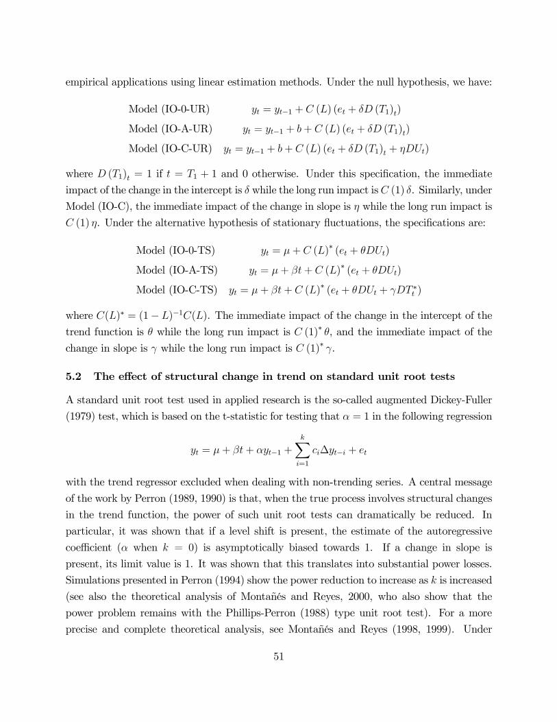
empirical applications using linear estimation methods. Under the null hypothesis, we have:

Model (IO-0-UR) yt = yt−1 + C (L) (et + δD (T1)t)

Model (IO-A-UR) yt = yt−1 + b+ C (L) (et + δD (T1)t)

Model (IO-C-UR) yt = yt−1 + b+ C (L) (et + δD (T1)t + ηDUt)

where D (T1)t = 1 if t = T1 + 1 and 0 otherwise. Under this specification, the immediate

impact of the change in the intercept is δ while the long run impact isC (1) δ. Similarly, under

Model (IO-C), the immediate impact of the change in slope is η while the long run impact is

C (1) η. Under the alternative hypothesis of stationary fluctuations, the specifications are:

Model (IO-0-TS) yt = µ+ C (L)∗ (et + θDUt)

Model (IO-A-TS) yt = µ+ βt+ C (L)∗ (et + θDUt)

Model (IO-C-TS) yt = µ+ βt+ C (L)∗ (et + θDUt + γDT ∗t )

where C(L)∗ = (1− L)−1C(L). The immediate impact of the change in the intercept of the

trend function is θ while the long run impact is C (1)∗ θ, and the immediate impact of the

change in slope is γ while the long run impact is C (1)∗ γ.

5.2 The effect of structural change in trend on standard unit root tests

A standard unit root test used in applied research is the so-called augmented Dickey-Fuller

(1979) test, which is based on the t-statistic for testing that α = 1 in the following regression

yt = µ+ βt+ αyt−1 +kXi=1

ci∆yt−i + et

with the trend regressor excluded when dealing with non-trending series. A central message

of the work by Perron (1989, 1990) is that, when the true process involves structural changes

in the trend function, the power of such unit root tests can dramatically be reduced. In

particular, it was shown that if a level shift is present, the estimate of the autoregressive

coefficient (α when k = 0) is asymptotically biased towards 1. If a change in slope is

present, its limit value is 1. It was shown that this translates into substantial power losses.

Simulations presented in Perron (1994) show the power reduction to increase as k is increased

(see also the theoretical analysis of Montañés and Reyes, 2000, who also show that the

power problem remains with the Phillips-Perron (1988) type unit root test). For a more

precise and complete theoretical analysis, see Montañés and Reyes (1998, 1999). Under

51

the null hypothesis, the large sample distribution is unaffected by the presence of a level

shift (Montañés and Reyes, 1999) and the test is asymptotically conservative in the presence

of a change in slope. It can, however, have a liberal size if the break occurs very early

in the sample (λ1 < .15) as documented by Leybourne et al. (1998) and Leybourne and

Newbold (2000). Intuitively, the latter result can be understood by thinking about the early

observations as outliers such that the series reverts back to the mean in effect for the rest

of the sample. The latter problem is, however, specific to the Dickey-Fuller (1979) type

unit root test, which is based on the conditional likelihood function, discarding the first

observations (see, Lee, 2000) 3. It has also been documented that the presence of stuctural

breaks in trend affects tests of the null hypothesis of stationarity (e.g., the Q or KPSS test)

by inducing size distortions towards rejecting the null hypothesis too often (e.g., Lee et al.,

1997). This is consistent with the effect on unit root tests in the sense that when trying to

distinguish the two hypotheses, the presence of structural changes induces a bias in favor of

the unit root representation.

It is important to discuss these results in relation to the proper way to specify alternative

unit root tests. The main result is that large enough changes in level and/or slope will induce

a reduction in the power of standard unit root tests. Small shifts, especially in level, are

likely to reduce power only slightly. Hence, what is important is to account for the large

shifts, not all of them if the others are small. Consider analyzing the US real GDP over, say,

the period 1900-1980. Within this sample, one can identify two shifts related to the 1929

crash (change in level) and the post 1973 productivity slowdown (change in slope). However

the post 73 sample would, here, consists of only a small proportion of the total sample and

the shift in slope in this period is unlikely to induce a bias and need not be accounted for.

Hence, the testing strategy discussed below need not make a statement about the precise

number of changes. It should rather be viewed as a device to remove biases induced by shifts

large enough to cause an important reduction in power.

5.3 Testing for a unit root allowing for changes at known dates.

The IO models under the null and alternative hypotheses can be nested in the a way which

specifies the regression from which the statistics will be constructed as follows:

yt = µ+ θDUt + βt+ γDT ∗t + δD (T1)t + αyt−1 +kXi=1

ci∆yt−i + et (29)

3Kim et al, 2004, study what happens when the trend regressor is absent and the series has a brokentrend with the coefficients on the trend and shift in slope shrinking to zero as the sample size increases.

52

for a value of the truncation lag parameter k chosen to be large enough as to provide a good

approximation (for methods on how to choose k, see Ng and Perron, 1995, 2001). For Model

(IO-0), the regressors (t,DT ∗t ) are not present, while for Model (IO-A), the regressor (DT ∗t )

is not present. The null hypothesis imposes the following restrictions on the coefficients.

For Model (IO—0), these are α = 1, θ = µ = 0 and, in general, δ 6= 0 (if there is a changein the intercept). For Model (IO-A), the restrictions are α = 1, β = θ = 0 and again, in

general, δ 6= 0, while for Model (IO-C), α = 1, β = γ = 0. Under the alternative hypothesis,

we have the following specifications: |α| < 1 and, in general, δ = 0. These restrictions are,

however, not imposed by most testing procedures. The test statistic used is the t-statistic

for testing the null hypothesis that α = 1 versus the alternative hypothesis that |α| < 1,

denoted tα(λ1) with λ1 = T1/T . It is important to note that, provided the specified break

date corresponds to the true break date, the statistic is invariant to the parameters of the

trend-function, including those related to the changes in level and slope (for an analysis of

the case when the break date is mis-specified, see Hecq and Urbain, 1993, Montañés, 1997,

Montañés and Olloqui, 1999, and Montañés et al., 2005, who also consider the effect of

choosing the wrong specification for the type of break). The limit distribution of the test

under the null hypothesis is

tα(λ1)⇒R 10W ∗(r, λ1)dW (r)hR 1

0W ∗(r, λ1)2dr

i1/2 (30)

where W ∗(r, λ1) is the residual function from a projection of a Wiener process W (r) on the

relevant continuous time versions of the deterministic components (1, 1(r > λ1) for Model(IO-0), 1, 1(r > λ1), r for Model (IO-A) and 1, 1(r > λ1), r, 1(r > λ1)(r− λ1) for Model(IO-C)). Tabulated critical values can be found in Perron (1989, 1990). See also Carrion i

Silvestre et al. (1999).

For the additive outlier models, the procedures are different and consist of a two-step

approach. In the first step, the trend function of the series is estimated and removed from

the original series via the following regressions for Model (AO-0) to (AO-C), respectively:

yt = µ+ γDUt + eytyt = µ+ βt+ γDUt + eytyt = µ+ βt+ γDT ∗t + eytyt = µ+ βt+ θDUt + γDT ∗t + eyt

53

where eyt is accordingly defined as the detrended series. The next step differs according towhether or not the first step involves DUt, the dummy associated with a change in intercept.

For Models (AO-0), (AO-A) and (AO-C), the test is based on the value of the t-statistic for

testing that α = 1 in the following autoregression:

eyt = αeyt−1 + kXj=0

djD (T1)t−j +kXi=1

ai∆eyt−i + et

Details about the need to introduce the current value and lags of the dummies D (Tb)t can

be found in Perron and Vogelsang (1992b). The limit distributions of the tests are then the

same as for the IO case. There is no need to introduce the dummies in the second step

regression for Model (AO-B) where no change in level is involved and the two segments of

the trend are joined at the time of break. The limit distribution is, however, different; see

Perron and Vogelsang (1993a, 1993b). Again, in all cases, the tests are invariant to the

change in level or slope provided the break date is correctly specified.

These unit root tests with known break dates have been extended in the following direc-

tions. Kunitomo and Sato (1995) derive the limit distribution of the likelihood ratio tests

for multiple structural changes in the AO case. Amsler and Lee (1995) consider a LM type

test in the context of a shift in level of the AO type. Saikkonen and Lütkepohl (2001) also

consider cases with a level shift of the AO type, though they allow for general forms of

shifts which can be indexed by some unknown parameter to be estimated. Following Elliott

et al. (1996), they propose a GLS-type detrending procedure, which is however based on

an AR(p) process for the noise. On the basis of simulation results, they recommend using

GLS detrending under the null hypothesis instead of a local alternative as done in Elliott

et al. (1996). Lanne et al. (2002) propose a finite sample modification which is akin to a

pre-whitening device. Let the detrended series be

yGLSt = yt − eµ− eγDUt − eβtand the estimate of the autoregressive polynomial of the first difference ∆ut be eb(L) (allestimates being obtained from the GLS procedure). With the filtered series defined asewt = eb(L)yGLSt , the test is then the t-statistic for testing that α = 1 in the regression

ewt = µ+ αewt−1 + πeb(L)D (T1)t + kXi=1

ai∆yGLSt−i + et.

Note that the limit distribution does not depend on the break date. This is because the

data are detrended using a GLS approach under the null hypothesis of a unit root (or more

54

generally under a sequence of alternatives that are local to a unit root) and the level shift

regressor is, in the terminology of Elliott et al. (1996), a slowly evolving trend, in which

case, the limit distribution is the same as it would be if it was excluded (loosely speaking,

the level shift becomes a one-time dummy). Hence, the limit distribution of the test is the

same as that of Elliott et al. (1996) for their unit root test when only a constant is included

as deterministic regressor. Lanne and Lütkepohl (2002) show that this test has better size

and power than the test proposed in Perron (1990) and the LM test of Amsler and Lee

(1995). A similar procedure for level shifts of the IO type is presented in Lütkepohl, Müller

and Saikkonen (2001).

5.4 Testing for a unit root allowing for changes at unknown dates

The methodology adopted by Perron (1989, 1990) was criticized by, among others, Christiano

(1992), on the ground that using a framework whereby the break is treated as fixed is

inappropriate. The argument is that the choice of the break date is inevitably linked to the

historical record and, hence, involves an element of data-mining. He showed that if one did

a systematic search for a break when the series is actually a unit root process without break,

using fixed break critical value would entail a test with substantial size distortions. While

the argument is correct, it is difficult to quantify the extent of the ‘data-mining’ problem in

Perron’s (1989) study. Indeed, no systematic search was done, the break dates were selected

as obvious candidates (the Crash of 1929 and the productivity slowdown after 1973) and the

same break date was used for all series. Given the intractability of correctly assessing the

right p-values for the tests reported, the ensuing literature addressed the problem by adopting

a completely agnostic approach where a complete and systematic search was done. While

this leads to tests with the correct asymptotic size (under some conditions to be discussed),

it obviously implies a reduction in power. We shall return to the practical importance of

this point.

An avenue taken by Banerjee et al. (1992) was to consider rolling and recursive tests.

Both perform standard unit root tests without breaks, the former using a sample of fixed

length (much smaller than the full sample) that moves sequentially from some starting date

to the end of the sample. The latter considers a fixed starting date for all tests and increases

the sample used (from some minimal value to the full sample). In each case, one then

considers the minimal value of the unit root test and rejects the null hypothesis of a unit

root if this minimal value is small enough. Asymptotically, such procedures will correctly

reject the null hypothesis if the alternative is true but the fact that all tests are based on

55

sub-samples means that not all information in the data is used and consequently one can

expect a loss of power.

An alternative strategy, more closely related to the methodology of Perron (1989) was

adopted by Zivot and Andrews (1992) as well as Banerjee et al. (1992). They consider the

IO type specification and a slightly different regression that does not involve the one-time

dummy when a shift in level is allowed under the alternative hypothesis. For example, for

Model C, the regression is

yt = µ+ θDUt + βt+ γDT ∗t + αyt−1 +kXi=1

ci∆yt−i + et (31)

and the test considered is the minimal value of the t-statistic for testing that α = 1 over

all possible break dates in some pre-specified range for the break fraction [ , 1 − ] where

a popular choice for is 0.15. Denote the resulting test by t∗α = infλ1∈[ ,1− ] tα(λ1) where

tα(λ1) is the t-statistic for testing α = 1 in (31) when the break date T1 = [Tλ1] is used.

The limit distribution of the test is

t∗α ⇒ infλ1∈[ ,1− ]

R 10W ∗(r, λ1)dW (r)hR 1

0W ∗(r, λ1)2dr

i1/2 (32)

withW ∗(r, λ1) as defined in (30). Perron (1997a) extended their theoretical results by show-

ing, using projection arguments, that trimming for the possible values of λ1 was unnecessary

and that one could minimize over all possible break dates 4. For the Nelson-Plosser (1982)

data set, Zivot and Andrews (1992) reported fewer rejections compared to what was reported

in Perron (1989) using a known break date assumption. These rejections should be viewed

as providing stronger evidence against the unit root but a failure to reject does not imply

a reversal of Perron’s (1989) conclusions. This is a commonly found mis-conception in the

literature, which overlooks the fact that a failure to reject may simply be due to tests with

low power.

Zivot and Andrews’ (1992) extension involves, however, a substantial methodological

difference. The null hypothesis considered is that of a unit root process with no break while

the alternative hypothesis is a stationary process with a break. Hence, there is an asymmetric

treatment of the specification of the trend under the null and alternative hypotheses. In

particular, limit result (32) is not valid if a break is present under the null hypothesis.

4Perron (1997a) also showed how the weak convergence result could be obtained using the usual supmetric instead of the hybrid metric adopted in Zivot and Andrews (1992).

56

Vogelsang and Perron (1998) show that, in this case, t∗α diverges to −∞ when a shift in

slope is present. This implies that a rejection can be due to the presence of a unit root

process with a breaking trend. The reason for this is the following. With a fixed break

date, the statistic tα(λ1) from regression (29) is invariant to the values of the parameters

of the trend function under both the null and alternative hypotheses. When searching over

a range of values for the break date (only one of which corresponding to the true value),

this invariance no longer holds. In the case of Model A with only a level shift and for

non-trending series with a change in mean considered by Perron and Vogelsang (1992a), the

statistic t∗α is asymptotically invariant to the value of the level shift but not in finite samples.

Simulations reported by Perron and Vogelsang (1992b) show size distortions that increase

with the magnitude of the level shift. They argue, however, that substantial size distortions

are in effect only when implausibly large shifts occur and that the problem is not important

in practice. Vogelsang and Perron (1998) make the same arguments for the case of a shift

in slope. Even though in practice the distortions may be small, it nevertheless remains a

problematic feature of this approach and we consider recent attempts below which do not

have this problem.

Perron and Vogelsang (1992a), for the non-trending case, and Perron (1997a), for the

trending case, extend the analysis of Zivot and Andrews (1992). They consider tests for

both the IO and AO cases based on the minimal value of the t-statistic for testing that

α = 1, and also tests based on tα(λ1) with T1 selected by maximizing the absolute value

of the t-statistic on the coefficient of the appropriate shift dummy, DUt if only a level shift

is present and DT ∗t if a slope change is present (see also Christiano, 1992, and Banerjee et

al., 1992). For the IO case, they also suggest using regression (29) instead of (31) which

includes the one-time dummy D (Tb)t since that would be the right regression to use with

a known break date. They derive the limit distribution under the null hypothesis of a

unit root and no break (in which case it does not matter if the one-time dummy D (Tb)tis incorporated). Perron (1997a) also considers tests where the break date is selected by

minimizing or maximizing the value of the t-statistic on the slope dummy, which allows

one to impose a priori the restriction of a direction for the change in slope and provides a

more powerful test. Carrion-i-Silvestre et al. (2004) consider statistics which jointly test

the null hypothesis and the zero value of appropriate deterministic regressors, extending the

likelihood ratio test of Dickey and Fuller (1981).

57

5.4.1 Extensions and other approaches

We now briefly review some extensions and alternative approaches and return below to

an assessment of the various methods discussed above. Unless stated otherwise, all work

described below specifies the null hypothesis as a unit root process with no break in trend.

Perron and Rodríguez (2003) consider tests for trending series with a shift in slope in

the AO framework. Following Elliott et al. (1996), they derive the asymptotic local power

envelop and show that using GLS detrended series (based on a local alternative) yields tests

with power close to the envelop. For the non-trending case, Clemente, Montañés and Reyes

(1998) extend the results of Perron and Vogelsang (1992a) to the case with two breaks. A

similar extension is provided by Lumsdaine and Papell (1997) for the case of trending series.

Generalizations to multiple breaks include the following. Ohara (1999) extends the Zivot

and Andrews (1992) approach to the general case with m breaks, though only critical values

for the two break case are presented. Ohara (1999) also proves an interesting generalization of

a result in Perron (1989) to the effect that, if a unit root test allowing form1 changes in slope

is performed on a series having m0 changes with m0 > m1, then the least-squares estimate

of α converges to one. This provides theoretical support for Rule 6 stated in Campbell and

Perron (1991), which states that ‘a non-rejection of the unit root hypothesis may be due to

misspecification of the deterministic components included as regressors’.

Kapetanios (2005) also deals with the multiple break case but considers the following

strategy, based on the sequential method of Bai (1997b) and Bai and Perron (1998) (see

section 3.5). First, denote the set of t-statistics for a unit root over all possible one break

partitions by τ 1. Choose the break date that minimizes the sum of squared residuals. Then

impose that break and insert an additional break over all permissible values (given some

imposed trimming) and store the associated unit root tests in the set τ 2, then choose the

additional break that minimizes the sum of squared residuals. Continue in this fashion until

an m break model is fitted and m sets of unit root tests are obtained. The unit root test

selected is then the one that is minimal over all m sets. The limit distribution is, however,

not derived, and the critical values are obtained through simulation with T = 250.

Saikonnen and Lütkepohl (2002) extend their tests for a level shift with a known break

date (of a general form possibly indexed by some unknown parameter) to the case of a shift

occurring at an unknown date. It can be performed in both the AO and IO frameworks and

the resulting procedure is basically the same as discussed in Section 5.3 for the known break

date case. This is because, with a GLS detrending procedure based on a specification that

is local to a unit root, the limit distribution of the test is the same whatever the break point

58

is selected to be. Hence, one can substitute any estimate of the break date without affecting

the limit null distribution of the test. They recommend using a unit root specification for

the detrending (as opposed to using a local alternative as in Elliott et al., 1996) since it leads

to tests with finite sample sizes that are robust to departures of the estimate of the break

date from its true value. Of course, power is highly sensitive to an incorrectly estimated

break date. Lanne et al. (2003) assess the properties of the tests when different estimates

of the break date are used. A substantial drawback of their approach is that they found the

test to have non-monotonic power, in the sense that the larger the shift in level the lower the

power in rejecting the unit root. Also, the power is sensitive to departures from the exact

specification for the type of change, and power can be reduced substantially if allowance is

made for a general shift indexed by some parameter when the shift is actually an abrupt

one.

Consider now testing the null hypothesis of stationarity. Tests of the type proposed by

Kwiatkowski et al. (1992) will reject the null hypothesis with probability one in large enough

samples if the process is affected by structural changes in mean and/or slope but is otherwise

stationary within regimes. This follows in an obvious way once one realizes that the KPSS

test is also a consistent test for structural change (see, nevertheless, simulations in Lee et al.,

1997). In order not to incorrectly reject the null hypothesis of stationarity, modifications are

therefore necessary. Kurozumi (2002), Lee and Strazicich (2001b) and Busetti and Harvey

(2001, 2003) consider testing the null hypothesis of stationarity versus the alternative of a

unit root in the presence of a single break for the specifications described above (see also,

Harvey and Mills, 2003). Their test is an extension of the Q-statistic of Gardner (1969), or

equivalently the KPSS test as discussed in Section 2. The test is constructed using least-

squares residuals from a regression incorporating the appropriate dummy variables. They

provide critical values for the known break date case. When the break is unknown, things

are less satisfactory. To ensure the consistency of the test, Lee and Strazicich (2001b) and

Busetti and Harvey (2001, 2003) consider the minimal value (as opposed to the maximal

value) of the statistics over all permissible break dates. Since the test rejects for large

values, this implies the need to resort to the value of the statistic at the break point that

permits the least-favorable outcome against the alternative. Hence, it results in a procedure

with low power. Kurozumi (2002) as well as Busetti and Harvey (2001, 2003) also consider

using the estimate of the break date that minimizes the sum of squared residuals from the

relevant regression under the null hypothesis. Since, the estimate of the break fraction is then

consistent, one can use critical values corresponding to the known break date case. They

59

show, however, that the need to estimate the break date induces substantial power losses.

Busetti (2002) extended this approach to a multivariate setting, where the null hypothesis

is that a set of series all share a common trend subject to a change and a stationary noise

function, the alternative being that one or more series have unit root noise components.

Also of related interest is the study by Kim et al. (2002) who study unit root tests with

a break in innovation variance following the work by Hamori and Tokihisa (1997). The issue

of unit roots and trend breaks has also been addressed using a Bayesian framework with

results that are generally in agreement with those of Perron (1989), see Zivot and Phillips

(1994), Wang and Zivot (2000) and Marriott and Newbold (2000).

5.4.2 Problems and recent proposals

Theoretical results by Vogelsang and Perron (1998) and simulation results reported in Perron

and Vogelsang (1992a), Lee and Strazicich (2001a), Harvey et al. (2001) and Nunes et al.

(1997) yield the following conclusions about the tests when a break is present under the null

hypothesis. For the IO case when a slope shift is present, both versions using the break date

by minimizing the unit root test or maximizing the absolute value of the t-statistic on the

coefficient of the slope dummy, yield tests with similar features, namely an asymptotic size

100%. In the presence of a level shift, the asymptotic size is correct but liberal distortions

occur when the level shift is large. When the one time dummy D (T1)t is included in the

regression, the source of the problem is that the break point selected with highest probability

(which increases as the magnitude of the break increases) is T 01 −1, i.e., one period before thetrue break; and it is for this choice of the break date that the tests have most size distortions.

Lee and Strazicich (2001a) show that the problem is the same as if the one time dummy

D (T1)t was excluded when considering the known break date case. Their result also implies

that, when unit root tests are performed using a regression of the form (31) without the one

time dummy D (T1)t, the correct break date is selected but the tests are still affected by size

distortions (which was also documented by simulations). In cases with only a level shift,

Harvey et al. (2001) suggest evaluating the unit root t-statistic at the break date selected

by maximizing the absolute value of the t-statistic on the coefficient of the level shift plus

one, and show that the tests then have correct size even for large breaks.

For the AO type models, the following features apply. When the break date is selected by

minimizing the unit root test, similar size distortions apply. However, when the break date

is selected by maximizing the absolute value of the t-statistic on the relevant shift dummy,

the tests have the correct size even for large breaks, and the correct break date is selected in

60

large samples. Vogelsang and Perron (1998) argue that the limit distribution of the unit root

tests is then that corresponding to the known break date case. They suggest, nevertheless,

to use the asymptotic critical values corresponding to the no break case since this leads to

a test having asymptotic size no greater than that specified for all magnitudes of the break,

even though this implies a conservative procedure when a break is present.

An alternative testing procedure, which naturally follows from the structural change

literature reviewed in Section 3, is to evaluate the unit root test at the break date selected

by minimizing the sum of squared residuals from the appropriate regression. Interesting

simulations pertaining to the IO case are presented in Lee and Strazicich (2001). They show

that if one uses the usual asymptotic critical values that apply for the no break case under

the null hypothesis, the tests are conservative when a break is present (provided the one

time dummy D (T1)t is included in the regression). They correctly note, however, that the

limit null distribution when no break is present depends on the limit distribution of the

estimated break date which may depend on nuisance parameters. Hatanaka and Yamada

(1999) present useful theoretical results for the IO regression (though they specify the data

generating process to be of the AO type). They show that, when a change in slope is present,

the estimate of the break fraction λ1, obtained by minimizing the sum of squared residuals,

is consistent and that the rate of convergence is T in both the I(1) and I(0) cases. They

also show that this rate of convergence is sufficient to ensure that the null limit distribution

of the unit root test is the same as when the break date is known. Hence, one need only

use the critical values for the known break date case that pertains to the estimated break

date. The test has accordingly more power since the critical values are smaller in absolute

value (they also consider a two break model and show the estimates of the break dates to

be asymptotically independent). The problem, however, is that the results apply provided

there is a break in the slope under the null hypothesis. Indeed, if no break is present, the

known break date limit distribution no longer applies; and if the break is small, it is likely

to provide a poor approximation to the finite sample distribution. Hatanaka and Yamada

(1999) present simulations results calibrated to slope changes in Japanese real GDP that

show the estimates of the break dates to have a distribution with fat tails and the unit root

test accordingly shows size distortions.

For the AO case, the work of Kim and Perron (2005) leads to the following results based

on prior work by Perron and Zhu (2005). Under the null hypothesis of a unit root, if a

slope change is present, the rate of convergence of the estimate of the break date obtained

by minimizing the sum of squared residuals is not fast enough to lead to a limit distribution

61

for the unit root tests (evaluated at this estimate of the break date) that is the same as in

the known break date case. They, however, show that a simple modification yields a similar

result as in the IO case. It involves performing the unit root test by trimming or eliminating

data points in a neighborhood of the estimated break date. This again leads to unit root

tests with higher power.

Let us summarize the above discussion. First, in the unknown break date case, the

invariance properties with respect to the parameters of the trend no longer apply as in the

known break date case. Popular methods based on evaluating the unit root test at the value

of the break date that minimizes it or maximizes the absolute value of the t-statistic on the

coefficient of the relevant dummy variable suffer from problems of liberal size distortions

when a large break is present (except with the latter method to select the break date in

the IO case) and little if any when the break is small. When the break is large, evaluating

the unit root test at the break date that minimizes the sum of squared residuals leads to a

procedure with correct size and better power. So this suggests a two step procedure that

requires in the first step a test for a change in the trend function that is valid whether a unit

root is present or not, i.e., under both the null and alternative hypotheses. In this context,

the work of Perron and Yabu (2005) becomes especially relevant. This is the approach taken

by Kim and Perron (2005). They use a pre-test for a change in trend valid whether the series

is I(1) or I(0). Upon a rejection, the unit root test is evaluated at the estimate of the break

date that minimizes the sum of squared residuals from the relevant regression. If the test

does not reject, a standard Dickey-Fuller test is applied. This is shown to yield unit root

tests with good size properties overall and better power. In cases where only level shifts are

present, similar improvements are possible even though, with a fixed magnitude of shift, the

estimate of the break date is not consistent under the null hypothesis of a unit root.

6 Testing for Cointegration Allowing for Structural Changes

We now discuss issues related to testing for cointegration when allowing for structural

changes. We first consider, in Section 6.1, single equation methods involving systems with

one cointegrating vector. Here tests have been considered with the null hypothesis as no-

cointegration and the alternative as cointegration, and vice versa. In Section 6.2, we consider

the multivariate case, where the issue is mainly determining the correct number of cointe-

grating vectors. Since many of the issues are similar to the case of testing for unit roots

allowing structural breaks, our discussion will be brief and outline the main results and

procedures suggested.

62

6.1 Single equation methods

Consider an n dimensional vector of variables yt = (y1t, y2t) with y1t a scalar, and y2t an

n− 1 vector. We suppose that the sub-system y2t is not cointegrated. Then the issue is to

determine whether or not there exists a cointegrating vector for the full system yt. Consider

the following static regression

y1t = α+ βy2t + ut (33)

The system is cointegrated if there exists a β such that the errors ut are I(0). Hence, a

popular method is to estimate this static regression by OLS and perform a unit root test

on the estimated residuals (see, Phillips and Ouliaris, 1990). Here the null hypothesis is

no-cointegration and the alternative is cointegration. Another approach is to use the Error

Correction Model (ECM) representation given by:

∆y1t = bzt−1 +kXi=1

di∆y2t + et

where zt = y1t − βy2t is the equilibrium error. In practice, one needs to replace β by an

estimate that is consistent when there is cointegration. The test can then be carried using

the t-statistic for testing that b = 0 (see, e.g., Banerjee et al., 1986).

When adopting the reverse null and alternative hypotheses, a statistic that has been

suggested is, again, Gardner’s (1969) Q test (see Shin, 1994). It can be constructed using

the OLS residuals from the static regression when the regressors are strictly exogenous, or,

more generally, the residuals from a regression augmented with leads and lags of the first-

differences of the regressors, as suggested by Saikkonen (1991) and Stock and Watson (1993).

Of course, many other procedures are possible.

Here, structural changes can manifest themselves in several ways. First, there can be

structural changes in the trend functions of the series without a change in the cointegrating

relationship (i.e., a change in the marginal distributions of the series). Campos et al. (1996)

have documented that shifts in levels do not affect the size of tests of the null hypothesis

of no cointegration, for both the ECM based test and the test based on the residuals from

the static regression. However, they affect the power of the latter, though not of the former.

If all regressors have a common break in the slope of their trend function, the tests can be

liberal and reject the null hypothesis of no-cointegration too often, though different tests

are affected differently (Leybourne and Newbold, 2003). This is related to what has been

labelled as co-breaking processes. Changes in the variance of the errors ut can also induce

size distortions if it occurs early enough in the sample (e.g., Noh and Kim, 2003).

63

Second, structural changes can manifest themselves through changes in the long-run rela-

tionship (33), either in the form of a change in the intercept, or a change in the cointegrating

vector. Here, the power of standard tests for the null hypothesis of no-cointegration can

have substantially reduced power as documented by Gregory et al. (1996) and Gregory and

Hansen (1996a).

An early contribution that proposed tests for the null hypothesis of no-cointegration

allowing for the possibility of a change in the long-run relation is that of Gregory and Hansen

(1996a). They extend the residual-based tests by incorporating appropriate dummies in

regression (33) and taking as the resulting test-statistic the minimal value over all possible

break dates. Cases covered are: 1) allowing a change in the level α; 2) allowing for a similar

change in level when regression (33) includes a time trend; 3) allowing for changes in both

the level α and the cointegrating vector β (with no trend); 4) the case allowing for a change

in the level and slope of an included trend and of the cointegrating vector is analyzed in

Gregory and Hansen (1986b). The limit distributions of the various tests are derived under

the null hypothesis that the series are not cointegrated and are individually I(1) processes

with a stable deterministic trend component. As in the case of tests for unit roots, the value

of the break date associated with the minimal value of a given statistic is not, in general, a

consistent estimate of the break date if a change is present. Cook (2004) shows the size of

the tests to be affected (towards excessive rejections) when the series are not cointegrated

and are individually I(1) processes with a change in trend.

The issue of allowing the possible change in trend under both the null and alternative

hypotheses does arise in the context of testing the null hypothesis of no-cointegration. Indeed,

under the null hypothesis, the model is a spurious one and the parameters of the cointegrating

vector are not identified. It might be possible to identify a change in the slope of a trend

under the null hypothesis, but this case is seldom of empirical interest. This means that no

further gains in power are possible by trying to exploit the fact that a change in specification

occurs under both the null and alternative hypotheses, as was done for unit root tests. Such

gains are, however, possible, when adopting cointegration as the null hypothesis.

Concerning tests that takes the null hypothesis to be cointegration, the contributions

include Bartley et al. (2001), Carrion-i-Silvestre and Sanso (2004) and Arai and Kurozumi

(2005). All are based on various modifications of Gardner’s (1969) Q statistic as used by Shin

(1994) without structural breaks. The general framework used is to specify the cointegrating

relationship by

y1t = α1 + α2(1 > T1) + γ1t+ γ2(t− T1)1(t > T1) + β1y2t + β1y2t1(t > T1) + ut (34)

64

The required residuals to construct theQ test are based on transformed regressions that allow

the construction of asymptotically optimal estimates of the cointegrating vector. Bartley et

al. (2001) consider only a change in the level and slope of the trend and use the canonical

cointegrating regression approach suggested by Park (1992) to estimate the cointegrating

vector β. The break date is selected by minimizing the sum of squared residuals from the

canonical cointegrating regression. They argue that the resulting estimate of the break

fraction is consistent and that the limit distribution of the test corresponds to that applying

in the known break date case. The simulations supports this assertion. Carrion-i-Silvestre

and Sanso (2004) and Arai and Kurozumi (2005) extend the analysis to cover more cases, in

particular allowing for a change in the cointegrating vector. In the case of strictly exogenous

regressors, they construct the Q test using residuals from the static regression (34) (scaled

appropriately with an estimate of the long-run variance of the errors, which allows for serial

correlation). In the general case without strictly exogenous regressors, both recommend using

the residuals from regression (34) augmented with leads and lags of the first-differences of

y2t (Carrion-i-Silvestre and Sanso (2004) show that the use of the Fully Modified estimates

of Phillips and Hansen (1990) leads to tests with very poor finite sample properties). Both

select the break date by minimizing the sum of squared residuals from the appropriate

regression, following the work of Kurozumi and Arai (2004) who show that the estimate of

the break fraction in this model converges at least at rate T 1/2. This permits limit critical

values corresponding to the known break date case. They also consider selecting the break

date as the value which minimizes the Q statistic but do not recommend its use given that

the resulting tests then suffers from large size distortions in finite samples.

A caveat about the approach discussed above is the fact that for the suggested methods

to be valid, there must be a change in the cointegrating relationship, if cointegration actually

holds. This is because the search for the potential break date is restricted to break fractions

that are bounded, in large samples, from the boundaries 0 and 1. Hence, when there is no

change the limit value cannot be 0 or 1, the estimate is inconsistent and has a non-degenerate

limit distribution, which in turn affects the limit distribution of the test (i.e., it does not

correspond to the one that would prevail if no break was present). But to ascertain whether

a break is present, one needs to know if there is cointegration, which is actually the object

of the test. Tests of whether a change in structure has occurred (as reviewed in Section 4.7)

will reject the null hypothesis of no change when a change actually occurs in a cointegrating

relationship, and will also reject if the system is simply not cointegrated. Hence, we are led

to a circular argument. The test procedure needs to allow for the possibility of a change and

65

not impose it. It may be possible to relax the restriction on the search for the break date

by allowing all possible values. In the context of cointegrated I(1) regressors, it is, however,

unknown at this point, if the estimate of the break fraction would converge to 0 or 1 when

no change is present.

6.2 Methods based on a mutivariate framework

We now consider tests that have been proposed when the variables are analyzed jointly as

a system. Here, the results available in the literature are quite fragmentary and much of it

pertains to a single break at a known date. Also, different treatments are possible by allowing

for a change in the trend function of the original series (i.e., the marginal processes), or in

allowing for a change in the cointegrating relation.

One of the early contribution is that of Inoue (1999). It allows for a one time shift in the

trend function of the series at some unknown date, either in level for non-trending series and

for both level and slope in trending series. He considers an AO type framework and also an

IO type regression when only a shift in intercept is allowed in the VAR. The specification

of the null and alternative hypotheses follow Zivot and Andrews (1992) and Gregory and

Hansen (1996), in that the shifts are allowed only under the alternative hypothesis. Hence,

the null hypothesis is that the system contains no break and no more than r cointegrating

vectors, and the alternative hypothesis is that the data can exhibit a change in trend and

that the cointegrating rank is r + 1, or greater than r. The breaks are assumed to occur at

the same date for all series. Under the alternative hypothesis, the series are not assumed to

be co-breaking, in the sense that the cointegrating vector that reduces the non-stationarity

in the stochastic component also eliminates the non-stationarity in the deterministic trend.

He considers the trace and maximal eigenvalue tests of Johansen (1988, 1991) with data

appropriately detrended allowing for a shift in trend, and the resulting statistic is based on

the maximal values over all permissible break dates. It is unclear what are the properties of

the tests when the null hypothesis is true with data that have broken trends. Also, although

the parameter r can be selected arbitrarily, the procedures cannot be applied sequentially to

determine the cointegrating rank of the system. This is because the breaks are not allowed

under the null hypothesis, only under the alternative. So if one starts with, say, r = 0, breaks

are allowed for alternatives such that the cointegrating rank is greater than 0. But, upon a

rejection, if one then wants to test the null of rank 1 versus an alternative with rank greater

than 1, one needs to impose no break under the null hypothesis of rank 1, a contradiction

from what was specified in the earlier step.

66

Saikkonen and Lütkepohl (2000a) also considers a test of the null hypothesis of r cointe-

grating vectors versus the alternative that this number is greater than r, allowing for a break

in the trend function of the individual series under both the null and alternative hypotheses.

They, however, only consider a level shift (in trending or non trending series) occurring at

some known date. To estimate the coefficients of the trend component of the series, they

use a similar GLS procedure, as discussed in Section 5.3, appropriately extended for the

multivariate nature of the problem. This detrending method imposes the null hypothesis.

Hence, the effect of level shifts is negligible in large samples and the limit distribution of the

test is the same as the standard (no-break) cointegration test of Lütkepohl and Saikkonen

(2000) and Saikkonen and Lütkepohl (2000b). Once the detrended data is obtained the test

is based on the eigenvalues of a reduced rank problem where restrictions implied by the

process and the breaks are not imposed.

Johansen et al. (2000) consider a more general problem but still with known break dates.

They consider multiple structural changes in the following VAR of order k,

∆yt = (Π,Πj)

⎛⎝ yt−1

t

⎞⎠+ µj +k−1Xi=1

Γi∆yt−i + et

for Tj−1 + k < t ≤ Tj for j = 1, ...,m. Hence, there are m breaks which can affect the

constant and the coefficients of the trend. Various tests for the rank of the cointegrating

matrix are proposed (imposing or not various restrictions on the deterministic components).

Since the estimates of the coefficients of the trend are estimated from a maximum-likelihood

type approach (following Johansen, 1988, 1991), the limit distribution depends on the exact

specification of the deterministic components and on the true break dates. Asymptotic

critical values are presented via a response surface analysis.

For the special case of a single shift in level, Lütkepohl et al. (2003) compare the two

approaches of Saikkonen and Lütkepohl (2000a) and Johansen et al. (2000). They show

that the former has higher local asymptotic power. However, the finite sample size-adjusted

power is very similar. They recommend using the method of Saikkonen and Lütkepohl

(2000a) on the basis of better size properties in finite samples and also on the fact that they

view having a limit distribution free of the break dates to be advantageous. A problem with

this argument is that the non-dependence of the limit distribution on the break date with

the procedure of Saikkonen and Lütkepohl (2000a) no longer holds in more general models,

especially when slope shifts are involved. Indeed, no result is yet available for this approach

with a GLS type detrending procedure when slope shifts are present.

67

Lütkepohl et al. (2004) extend the analysis of Saikkonen and Lütkepohl (2002), which

pertained to testing for a unit root allowing for a change in the level of a series occurring

at an unknown date (see Section 5.4.1). The GLS type procedure discussed above is used

to estimate the coefficients of the deterministic components. Once the series are detrended,

the cointegration tests of Johansen (1988) can be used. In the unit root case, with a GLS

detrending procedure that imposes the null hypothesis, the change in mean reduces to an

outlier in the first-differenced series. Here, thing are more complex and a consistent estimate

of the break date is preferable. Estimating the break date has, however, no effect on the

limit null distribution of the test statistic since, here again, it does not depend on the true

value of the break date.

In it useful to consider in more detail the issue of estimating the break date. The n vector

of data yt is assumed to be generated by

yt = µ+ θDUt + δt+ xt

where DUt = 1(t > T1) and xt is a noise component generated by a VAR, with the following

ECM representation,

∆xt = Πxt−1 +kXi=1

Γi∆xt−i + et

Here, the presence of cointegration implies the decomposition Π = αβ0 with β the n × r

matrix of cointegrating vectors. Hence, we also have the following ECM representation for

yt

∆yt = ν + αβ0 (yt−1 − δ(t− 1)− θDUt−1) +kXi=1

Γi∆yt−i +kXi=1

γi∆DUt−i + et (35)

This ECM representation will be affected by a level shift if β0θ 6= 0, otherwise only the

impulse dummies ∆DUt−i are present. In most cases of interest, we have β0δ = 0, which

specifies that the same linear combinations that eliminate the stochastic non-stationarity

also eliminate the non-stationarity induced by the trend. The condition β0θ = 0 can be

interpreted in the same way, i.e., if some variables are affected by changes in trend, the

linear combination of the data specified by the cointegrating vectors will be free of structural

breaks. This is often referred to as ‘co-breaking’. Hence, the condition β0θ 6= 0 requires

that the series be non co-breaking, which may be unappealing in many cases. Lütkepohl et

al. (2004) estimate the break date by minimizing the determinant of the sample covariance

matrix of the estimates of the errors et. They show the estimate of the break fraction to

68

converge at rate T , though no limit distribution is given since this rate is enough to guarantee

that the limit distribution of the test be independent of the break date. Note that the search

for the break date is restricted to an interval that excludes a break fraction occurring near

the beginning or the end of the sample. This is important, since it makes the procedure

valid conditional on shifts in level occurring. Without shifts, the true break fraction is 0 or

1, which are excluded from the search. Hence, in this case the estimated break fractions will

converge to some random variable. But given that a GLS type detrending is done, this has

no impact of the limit distribution of the rank test. A similar result holds when co-breaking

shifts are present, though Lütkepohl et al. (2004) argue that if the shifts are large enough,

they can be captured by the impulse dummies ∆DUt−i (for more details on estimation of

break dates in this framework, see Saikkonen et al., 2004).

All contributions discussed above do not address the problem of a potential shift in the

cointegrating vector. A recent analysis by Andrade et al. (2005) deals with this in the

context of a one-time change. The object is to test the null hypothesis of r cointegrating

vectors versus the alternative that this value is greater than r. They allow the change in

the cointegrating relationship to occur under both the null and alternative hypotheses and

the number of cointegrating vectors is the same in both regimes. This allows a sequential

procedure to determine the rank. The issues are addressed using the following generalized

ECM

∆yt = 1(t ≤ T1)[α0β00yt−1 − δ0dt] + 1(t > T1)[α1β

01(yt−1 − yT1)− δ1dt] +

kXi=1

Γi∆yt−i + et

where dt is a vector of deterministic components (usually the null set or a constant). Note

that the data is re-normalized after the break to start again at 0. This is done since otherwise

the variance of β01yt−1 would increase after the break given that it depends on the value

of β01yT1. They note that the estimation of this model by maximum likelihood is quite

involved and suggest a simpler principle components analysis. Let βi⊥ be a matrix such that

β0iβi⊥ = 0, and suppose that the loading factors (or adjustment matrices) are constant, i.e.,

α0 = α1, the test for the null hypothesis that the cointegrating rank is r is based on testing

that γ0 = γ1 = 0 in the following system

∆yt = 1(t ≤ T1)hγ0β

00⊥yt−1 + αβ

00yt−1

i+ 1(t > T1)

hγ1β

01⊥yt−1 + αβ

01(yt−1 − yT1)

i+

kXi=1

Γi∆yt−i + et

69

where β01 and β

0i⊥ are estimates obtained from the principle components analysis. The

statistic is based on a multivariate Fisher-type statistic modified to eliminate the effect of

nuisance parameters on the limit distribution under the null hypothesis. They also consider

a version that is valid when the break date is unknown, based on the maximal values over

a specified range for the break date, and present a test to evaluate how many cointegrating

vectors are subject to change across regimes. When both the cointegrating matrix β and the

loading factors α are allowed to change, a more involved testing procedure is offered, which

applies, however, only to the known break date case.

An interesting recent contribution is that of Qu (2004). It proposes a procedure to

detect whether cointegration (or stationarity in the scalar case) is present in any part of the

sample, more precisely whether there is evidence in any part of the sample that a system

is cointegrated with a higher cointegrating rank than the rest of the sample. The test

procedure is based on a multivariate generalization of Gardner’s (1969) Q test as used in

Breitung (2002). The main device used is that if one or more sub-samples have a different

cointegrating rank, one can find them by searching, in an iterative fashion, over all possible

partitions of the sample with three segments or two breaks. The relevant limit distributions

are derived allowing the possibility of imposing some structure if desired (e.g., that the

change occurs at the beginning or end of the sample). He also discusses how to consistently

estimate the break dates or the boundaries of the regimes when a change has been detected.

A modification is also suggested to improve the finite sample performance of the test. This

approach also permit testing for changes in persistence with the null hypothesis specified as

an I(1) process throughout the sample. It also permits detecting whether cointegration is

present when the cointegrating vector changes at some unknown possibly multiple dates.

7 Conclusions

This review has discussed a large amount of research that has been done in the last fif-

teen years or so pertaining to issues related to structural changes and to try to distinguish

between structural changes and unit roots. But still, some important questions remain to

be addressed: limit distributions of estimates of break dates in a cointegrated system with

multiple structural changes, issues of non-monotonic power functions for tests of structural

change and how to alleviate the problems, evaluating the frequency of permanent shocks;

just to name a few. Research currently under progress is trying to address these and other

issues.

One recent area of research where similar tools have been applied is related to distinguish-

70

ing between long-memory processes and short-memory processes with structural changes, in

particular level shifts. This is especially important in financial economics, where it is widely

documented that various measures of stock return volatility exhibit properties similar to

those of a long-memory process (e.g., Ding et al., 1993, Granger and Ding, 1995 and Lobato

and Savin, 1998). For reviews of the literature on purely long-memory processes, see Robin-

son (1994a), Beran (1994) and Baillie (1996). A mentioned in Section 2, a popular test for

long-memory is the rescaled-range test. Yet, interestingly, Gardner’s (1969) Q test makes

yet another appearance. Indeed, it was, along with a slight modification, also proposed to

test this problem by Giraitis et al. (2003). So we have the same test acting with the null hy-

pothesis of a stable short-run memory process versus an alternative that is either structural

change, a unit root or long-memory. This goes a long way showing how the three problems

are inter-related.

One of the most convincing evidence that stock market volatility may be better charac-

terized by a short-memory process affected by occasional level shifts is that of Perron and Qu

(2004). They show that the behavior of the log-periodogram estimate of the long-memory

parameter (the fractional differencing coefficient), as a function of the number of frequencies

used in the regression, is very different for the two types of processes. The pattern found

with data on daily SP500 return series (absolute or square root returns) is very close to what

is expected with a short-memory process with level shifts. They also present a test which

rejects the null hypothesis of long memory.

Given that unit root and long memory processes share similar features, it is not surprising

that many of the same problems are being addressed with similar findings. Along the lines of

Perron (1989) for unit roots, it has been documented that short-memory processes with level

shifts will exhibit properties that make standard tools conclude that long memory is present

(e.g., Diebold and Inoue, 2001, Engle and Smith, 1999, Gourieroux and Jasiak, 2001, Granger

and Ding, 1996, Granger and Hyung, 2004, Lobato and Savin, 1998, and Teverosovky and

Taqqu, 1997). Some papers have also documented the fact that long-memory processes will

induce, similar to unit root processes, a rejection of the null hypothesis of no-structural

change when using standard structural change tests; for the CUSUM and the Sup-Wald test

applied to a change in a polynomial trend, see Wright (1998) and Krämer and Sibbertsen

(2002).

Results about the rate of convergence of the estimated break fraction in a single mean

shift model can be found in Kuan and Hsu (1998). When there is structural change, the

estimate is consistent but the rate of convergence depends on d. When d ∈ (0, 1/2) and

71

there is no change, the limit value is not 0 or 1 but rather the estimate of the break fraction

converges to a random variable, suggesting a spurious change, exactly as in the unit root

case (see Nunes et al., 1995, and Bai, 1998). For results related to multiple structural

changes in mean, see Lavielle and Moulines (2000). A test for a single structural change

occurring at some known date in the linear regression model is discussed in Hidalgo and

Robinson (1996). It is essentially a Wald test for testing that the coefficients are the same

in both regimes, which accounts for the long-memory correlation pattern in the residuals.

Lazarová (2005) presents a test for the case of a single change in the parameters of a linear

regression model occurring at an unknown date. The test follows the “fluctuations tests”

approach of Ploberger et al. (1989) with different metrics used to weight the differences

in the estimates for each permissible break dates (giving special attention to the Sup and

Mean functionals). The limit distribution depends on nuisance parameters and a bootstrap

procedure is suggested to obtain the relevant critical values.

Related to the problem of change in persistence (see Section 4.9), Beran and Terrin (1996)

present a test for a change in the long-memory parameter, based on the maximal difference,

across potential break dates, of appropriately weighted sums of autocovariances. Related

to unit root tests allowing for a change in the trend function, Gil-Alana (2004) extends

Robinson’s (1994b) test to allow for a one-time change occurring at a known date. For a

review of some related results, see Sibbertsen (2004).

The literature on structural changes in the context of long memory processes is quite

new and few results are available. Still, there is a large demand for empirical applications.

Given the nature of the problems and series analyzed, it is important to have procedures

that are valid for multiple structural changes. For example, with many financial time series,

it is the case that allowing for structural breaks reduces considerably the estimates of the

long-memory parameters within regimes (e.g., Granger and Hyung, 2004, for stock return

volatility). Are the reductions statistically significant? Are the reductions big enough that

one can consider the process as being of a short-memory nature within regimes? Is there sig-

nificant evidence of structural changes? Is the long-memory parameter stable across regimes?

The econometrics and statistics literatures have a long way to go to provide reliable tools

to answer these questions. Given that the issues are similar to the structural change versus

unit root problem, our hope is that this survey will provide a valuable benchmark to direct

research in specific directions and to alert researchers of the potential merits and drawbacks

of various approaches.

72

References

[1] Altissimo, F., Corradi, V., 2003. Strong rules for detecting the number of breaks in atime series. Journal of Econometrics 117, 207-244.

[2] Amsler, C., Lee, J., 1995. An LM test for a unit root in the presence of a structuralchange. Econometric Theory 11, 359-368.

[3] Anderson, T.W., Darling, D.A., 1952. Asymptotic theory of certain ‘goodness of fit’criteria based on stochastic processes. The Annals of Mathematical Statistics 23, 193-212.

[4] Andrade, P., Bruneau, C., Gregoir, S., 2005. Testing for the cointegration rank whensome cointegrating directions are changing. Journal of Econometrics 124, 269-310.

[5] Andrews, D.W.K., 1991. Heteroskedasticity and autocorrelation consistent covariancematrix estimation. Econometrica 59, 817-858.

[6] Andrews, D.W.K., 1993a. Tests for parameter instability and structural change withunknown change point. Econometrica 61, 821-856 (Corrigendum, 71, 395-397).

[7] Andrews, D.W.K., 1993b. Exactly median-unbiasedestimation of first-order autore-gressive/unit root models. Econometrica 61, 139-165.

[8] Andrews, D.W.K., Lee, I., Ploberger, W., 1996. Optimal change point tests for normallinear regression. Journal of Econometrics 70, 9-38.

[9] Andrews, D.W.K., Ploberger, W., 1994. Optimal tests when a nuisance parameter ispresent only under the alternative. Econometrica 62, 1383-1414.

[10] Antoch, J., Hušková, M., Prášková, Z., 1997. Effect of dependence on statistics fordetermination of change. Journal of Statistical Planning and Inference 60, 291-310.

[11] Arai, Y., Kurozumi, E., 2005. Testing the null hypothesis of cointegration with struc-tural breaks. Unpublished manuscript, Hitotsubashi University.

[12] Bai, J., 1994. Least squares estimation of a shift in linear processes. Journal of TimeSeries Analysis 15, 453-472.

[13] Bai, J., 1997a. Estimation of a change point in multiple regression models. Review ofEconomic and Statistics 79, 551-563.

[14] Bai, J., 1997b. Estimating multiple breaks one at a time. Econometric Theory 13,315-352.

[15] Bai, J., 1998. A note on spurious break. Econometric Theory 14, 663-669.

[16] Bai., J., 1999. Likelihood ratio tests for multiple structural changes. Journal of Econo-metrics 91, 299-323.

73

[17] Bai, J., 2000. Vector autoregressive models with structural changes in regression co-efficients and in variance-covariance matrices. Annals of Economics and Finance 1,303-339.

[18] Bai, J., Lumsdaine, R.L., Stock, J.H., 1998. Testing for and dating breaks in multi-variate time series. Review of Economic Studies 65, 395-432.

[19] Bai, J., Perron, P., 1998. Estimating and testing linear models with multiple structuralchanges. Econometrica 66, 47-78.

[20] Bai, J., Perron, P., 2003a. Computation and analysis of multiple structural changemodels. Journal of Applied Econometrics 18, 1-22.

[21] Bai, J., Perron, P., 2003b. Critical values for multiple structural change tests. Econo-metrics Journal 6, 72-78.

[22] Bai, J., Perron, P., 2005. Multiple structural change models: a simulation analysis.Forthcoming in Econometric Essays, D. Corbea, S. Durlauf and B. E. Hansen (eds.),Cambridge University Press.

[23] Baillie, R.T., 1996. Long memory processes and fractional integration in econometrics.Journal of Econometrics 73, 5-59.

[24] Banerjee, A., Dolado, J.J., Hendry, D.F., Smith, G.W., 1986. Exploring equlibrium re-lationships in econometrics through static models: some Monte Carlo evidence. OxfordBulletin of Economics and Statistics 48, 253-277.

[25] Banerjee, A., Lumsdaine, R.L., Stock, J.H., 1992. Recursive and sequential tests of theunit-root and trend-break hypotheses: theory and international evidence. Journal ofBusiness and Economic Statistics 10, 271-287.

[26] Barsky, R.B., 1987. The Fisher hypothesis and the forecastibility and persistence ofinflation. Journal of Monetary Economics 19, 3-24.

[27] Bartley, W.A., Lee, J., Strazicich, M.C., 2001, Testing the null of cointegration in thepresence of a structural break. Economics Letters 73, 315-323.

[28] Bellman, R., Roth, R., 1969. Curve fitting by segmented straight lines. Journal of theAmerican Statistical Association 64, 1079-1084.

[29] Beran, J., 1994. Statistics for Long Memory Processes. New York: Chapman & Hall.

[30] Beran, J., Terrin, N., 1996. Testing for a change of the long-memory parameter.Biometrika 83, 627-638.

[31] Beveridge, S., Nelson, C.R., 1981. A New Approach to Decomposition of EconomicTime Series into Permanent and Transitory Components with Particular Attention toMeasurement of the ‘Business Cycle’. Journal of Monetary Economics 7, 151-74.

74

[32] Bhattacharya, P.K., 1987. Maximum likelihood estimation of a change-point in thedistribution of independent random variables, general multiparameter case. Journal ofMultivariate Analysis 23, 183-208.

[33] Bhattacharya, P.K., 1994. Some aspects of change-point analysis. In Carlstein, E.,Müller, H.-G., Siegmund, D. (eds.), Change Point Problems, IMS Lecture Notes -Monograph Series, vol. 23, 28-56.

[34] Bhattacharya, R.N., Gupta, V.K., Waymire, E., 1983. The Hurst effect under trends.Journal of Applied Probability 20, 649-662.

[35] Box, G.E.P., Tiao, G.C., 1975. Intervention analysis with applications to economic andenvironmental problems. Journal of the American Statistical Association 70, 70-79.

[36] Breitung, J., 2002. Nonparametric tests for unit roots and cointegration. Journal ofEconometrics 108, 343-363.

[37] Brown, R.L., Durbin, J., Evans, J.M., 1975. Techniques for testing the constancy ofregression relationships over time. Journal of the Royal Statistical Society B 37, 149-163.

[38] Burdekin, R.C.K., Siklos, P.L., 1999. Exchange rate regimes and shifts in inflationpersistence: does nothing else matter?. Journal of Money, Credit and Banking 31,235-247.

[39] Busetti, F., 2002. Testing for (common) stochastic trends in the presence of structuralbreaks. Journal of Forecasting 21, 81-105.

[40] Busetti, F., Harvey, A.C., 2001. Testing for the presence of a random walk in serieswith structural breaks. Journal of Time Series Analysis 22, 127-150.

[41] Busetti, F., Harvey, A.C., 2003. Further comments on stationarity tests in series withstructural breaks at unknown points. Journal of Time Series Analysis 24, 137-140.

[42] Busetti, F., Taylor, A.M.R., 2001. Tests stationarity against a change in persistence.Discussion Paper 01-13, Department of Economics, University of Birmingham.

[43] Busetti, F., Taylor, A.M.R., 2005. Tests stationarity against a change in persistence.Journal of Econometrics. Forthcoming.

[44] Campbell, J.Y., Perron, P., 1991. Pitfalls and opportunities: what macroeconomistsshould know about unit roots. NBER Macroeconomics Annual, Vol. 6, Blanchard,O.J., Fisher, S. (eds.), 141-201.

[45] Campos, J., Ericsson, N.R., Hendry, D.F., 1996. Cointegration tests in the presence ofstructural breaks. Journal of Econometrics 70, 187-220.

75

[46] Carion-i-Silvestre, J.L., Sansó-i-Rosselló, A.S., 2004. Testing the null hypothe-sis of cointegration with structural breaks. Unpublished manuscript, Departamentd’Econometria, Estadística i Economia Espanyola, Universitat de Barcelona.

[47] Carion-i-Silvestre, J.L., Sansó-i-Rosselló, A.S., Artis, M., 2004. Joint hypothesis spec-ification for unit root tests with a structural break. Unpublished manuscript, Depar-tament d’Econometria, Estadística i Economia Espanyola, Universitat de Barcelona.

[48] Carion-i-Silvestre, J.L., Sansó-i-Rosselló, A.S., Ortuño, M.A., 1999. Response surfaceestimates for the Dickey-Fuller test with structural breaks. Economics Letters 63, 279-283.

[49] Chernoff, H., Zacks, S., 1964. Estimating the current mean of a normal distributionwhich is subject to changes in time. The Annals of Mathematical Statistics 35, 999-1018.

[50] Chong, T.T.L., 1995. Partial parameter consistency in a misspecified structural changemodel. Economics Letters 49, 351-357.

[51] Chong, T.T.L., 2001. Structural change in AR(1) models. Econometric Theory 17,87-155.

[52] Christiano, L.J., 1992. Searching for breaks in GNP. Journal of Business and EconomicStatistics 10, 237-250.

[53] Chu, C.-S.J., Hornik, K., Kuan, C.-M., 1995. MOSUM tests for parameter constancy.Biometrika 82, 603-617.

[54] Chu, C.-S. J., White, H., 1992, A direct test for changing trend. Journal of Businessand Economic Statistics 10, 289-299.

[55] Clemente, J., Montañés, A., Reyes, M., 1998. Testing for a unit root in variables witha double change in the mean. Economics Letters 59, 175-182.

[56] Clements, M.P., Hendry, D.F., 1999. Forecasting Non-stationary Economic Time Se-ries. MIT Press, Cambridge, MA.

[57] Cook, S., 2004. Spurious rejection by cointegration tests incorporating structuralchange in the cointegrating relationship. Unpublished manuscript, Department of Eco-nomics, University of Wales Swansea.

[58] Crainiceanu, C.M., Vogelsang, T.J., 2001. Spectral density bandwidth choice: source ofnonmonotonic power for tests of a mean shift in a time series. Unpublished manuscript,Department of Economics, Cornell University.

[59] Csörgo, M., Horváth, L., 1997. Limit theorems in change-point analysis. Wiley Seriesin Probability and Statistics, New York: John Wiley.

76

[60] Davies, R.B., 1977. Hypothesis testing when a nuisance parameter is present onlyunder the alternative. Biometrika 64, 247-254.

[61] Davies, R.B., 1987. Hypothesis testing when a nuisance parameter is present onlyunder the alternative. Biometrika 74, 33-43.

[62] DeLong, J.B., Summers, L.H., 1988. How does macroeconomic policy affect output?.Brookings Papers on Economic Activity 2, 433-494.

[63] Deng, A., Perron, P., 2005a. A comparison of alternative asymptotic frameworks to an-alyze structural change in a linear time trend. Manuscript in preparation, Departmentof Economics, Boston University.

[64] Deng, A., Perron, P., 2005b. A locally asymptotic point optimal test that is incon-sistent: the case of a change in persistence. Unpublished manuscript, Department ofEconomics, Boston University.

[65] Deshayes, J., Picard, D., 1984a. Principe d’invariance sur le processus de vraisem-blance. Annales de l’Institut Henri Poincaré, Probabilités et Statistiques 20, 1-20.

[66] Dehayes, J., Picard, D., 1984b. Lois asymptotiques des tests et estimateurs de rupturedans un modèle statistique classique. Annales de l’Institut Henri Poincaré, Probabilitéset Statistiques 20, 309-327.

[67] Deshayes, J., Picard, D., 1986. Off-line statistical analysis of change point modelsusing non-parametric and likelihood methods. In Basseville, M., Beneviste, A., (eds),Detection of Abrupt Changes in Signals and Dynamical Systems (Lecture Notes inControl and Information Sciences 77), 103-168, Berlin: Springer.

[68] Dickey, D.A., Fuller, W.A., 1979. Distribution of the estimators for autoregressive timeSeries with a unit Root. Journal of the American Statistical Association 74, 427-431.

[69] Dickey, D.A., Fuller, W.A., 1981. Likelihood ratio statistics for autoregressive timeseries with a unit root. Econometrica 49, 1057-1072.

[70] Diebold, F., Inoue, A., 2001. Long memory and regime switching. Journal of Econo-metrics 105, 131-159.

[71] Ding, Z., Engle, R.F., Granger, C.W.J., 1993. A long memory property of stock marketreturns and a new model. Journal of Empirical Finance 1, 83-106.

[72] Dufour, J.M., 1982. Recusrive stability analysis of linear regression relationships: anexploratory methodology. Journal of Econometrics 19, 31-76.

[73] Dufour, J.-M., Kiviet, J.F., 1996. Exact tests for structural change in first-order dy-namic models. Journal of Econometrics 70, 39-68.

77

[74] Elliott, G., Müller, U.K., 2003. Optimally testing general breaking processes in lineartime series models. Unpublished manuscript. Department of Economics, University ofCalifornia at San Diego.

[75] Elliott, G., Müller, U.K., 2004. Confidence sets for the date of a single break in lineartime series regressions. Unpublished manuscript, Department of Economics, Universityof California at San Diego.

[76] Elliott, G., Rothenberg, T.J., Stock, J.H., 1996. Efficient tests for an autoregressiveunit root. Econometrica 64, 813-836.

[77] Engle, R.F., Smith, A.D., 1999. Stochastic permanent breaks. Review of Economicsand Statistics 81, 533-574.

[78] Feder, P.I., 1975. On asymptotic distribution theory in segmented regression problems:identified case. Annals of Statistics 3, 49-83.

[79] Fisher, W.D., 1958. On grouping for maximum homogeneity. Journal of the AmericanStatistical Association 53, 789-798.

[80] Fu, Y-X., Curnow, R.N., 1990. Maximum likelihood estimation of multiple changepoints. Biometrika 77, 563-573.

[81] Garcia, R., Perron, P., 1996. An analysis of the real interest rate under regime shifts.Review of Economics and Statistics 78, 111-125.

[82] Gardner, L.A., 1969. On detecting changes in the mean of normal variates. The Annalsof Mathematical Statistics 40, 116-126.

[83] Giraitis, L., Kokoszka, P., Leipus, R., Teyssière, G., 2003. Rescaled variance and relatedtests for long memory in volatility and level. Journal of Econometrics 112, 265-294(Corrigendum, 126, 571-572).

[84] Gil-Alana, L.A., 2004. A joint test of fractional integration and structural breaks at aknown period of time. Journal of Time Series Analysis 25, 691-700.

[85] Gourieroux, C., Jasiak, J., 2001. Memory and infrequent breaks. Economics Letters70, 29-41.

[86] Granger, C.W.J., Ding, Z., 1996. Varieties of long memory models. Journal of Econo-metrics 73, 61-77.

[87] Granger, C.W.J., Hyung N., 2004. Occasional structural breaks and long memory withan application to the S&P 500 absolute stock returns. Journal of Empirical Finance11, 399-421.

[88] Gregory, A.W., Hansen, B.E., 1996a. Residual-based tests for cointegration in modelswith regime shifts. Journal of Econometrics 70, 99-126.

78

[89] Gregory, A.W., Hansen, B.E., 1996b. Tests for cointegration in models with regimeand trend shifts. Oxford Bulletin of Economics and Statistics 58, 555-560.

[90] Gregory, A.W., Nason, J.M., Watt, D.G., 1996. Testing for structural breaks in coin-tegrated relationships. Journal of Econometrics 71, 321-341.

[91] Guthery, S.B., 1974. Partition Regression. Journal of the American Statistical Associ-ation 69, 945-947.

[92] Hackl, P., Westlund, A.H., 1989. Statistical analysis of ‘structural change’: an anno-tated bibliography. Empirical Economics 14, 167-192.

[93] Hackl, P., Westlund, A.H., 1991 eds. Economic Structural Change: Analysis and Fore-casting. Springer-Verlag: Berlin.

[94] Hakkio, C.S.., Rush, M., 1991. Is the budget deficit too large?. Economic Inquiry 29,429-445.

[95] Hall, A.R., 2005. Generalized Methods of Moments. Oxford University Press.

[96] Hamori, S., Tokihisa, A., 1997. Testing for a unit root in the presence of a varianceshift. Economics Letter 57, 245-253.

[97] Hansen, B.E., 1992a. Tests for parameter instability in regressions with I(1) processes.Journal of Business and Economic Statistics 10, 321-335.

[98] Hansen, B.E., 1992b. Testing for parameter instability in linear models. Journal ofPolicy Modeling 14, 517-533.

[99] Hansen, B.E., 1996. Inference when a nuisance parameter is not identified under thenull hypothesis. Econometrica 64, 413-430.

[100] Hansen, B.E., 2000. Testing for structural change in conditional models. Journal ofEconometrics 97, 93-115.

[101] Hansen, H., Johansen, S., 1999. Some tests for parameter constancy in cointegratedVAR-models. Econometrics Journal 306-333.

[102] Hansen, P.R., 2003. Structural changes in the cointegrated vector autoregressive model.Journal of Econometrics 114, 261-295.

[103] Harvey, D.I., Leybourne, S.J., Taylor, A.M.R., 2004. Modified tests for a change inpersistence. Unpublished manuscript, Department of Economics, University of Birm-ingham.

[104] Hájek, J., Rényi, A., 1955. Generalization of an inequality of Kolmogorov. Acta Math.Acad. Sci. Hungar. 6, 281-283.

79

[105] Hao, K., 1996. Testing for structural change in cointegrated regression models: somecomparisons and generalizations. Econometric Reviews 15, 401-429.

[106] Hao, K., Inder, B., 1996. Diagnostic test for structural change in cointegrated regressionmodels. Economics Letters 50, 179-187.

[107] Harvey, A.C., 1975. Comment on the paper by Brown, Durbin and Evans. Journal ofthe Royal Statistical Society B 37, 179-180.

[108] Harvey, D.I., Leybourne, S.J., Newbold, P., 2001. Innovational outlier unit root testswith an endogeneously determined break in level. Oxford Bulletin of Economics andStatistics 63, 559-575.

[109] Harvey, D.I., Mills, T.C., 2003. A note on Busetti-Harvey tests for stationarity in serieswith structural breaks. Journal of Time Series Analysis 24, 159-164.

[110] Hatanaka, M., Yamada, K., 1999. A unit root test in the presence of structural changesin I(1) and I(0) Models. In Cointegration, Causality, and Forecasting: A Festschrift inHonour of Clive W.J. Granger, Engle, R.F., White, H., eds., Oxford University Press.

[111] Hatanaka, M., Yamada, K., 2003. Co-trending: A Statistical System Analysis of Eco-nomic Trends. Springer-Verlag: Tokyo.

[112] Hawkins, D.L., 1987. A test for a change point in a parametric model based on amaximal Wald-type statistic. Sankhya 49, 368-376.

[113] Hawkins, D.M., 1976. Point estimation of the parameters of piecewise regression mod-els. Applied Statistics 25, 51-57.

[114] Hawkins, D.M., 1977. Testing a sequence of observations for a shift in location. Journalof the American Stastistical Association 72, 180-186.

[115] Hecq, A., Urbain, J.P., 1993. Misspecification tests, unit roots and level shifts. Eco-nomics Letters 43, 129-135.

[116] Hidalgo, J., Robinson, P.M., 1996. Testing for structural change in a long-memoryenvironment. Journal of Econometrics 70, 159-174.

[117] Hinkley, D.V., 1970. Inference about the change-point in a sequence of random vari-ables. Biometrika 57, 1-17.

[118] Horváth, L., 1995. Detecting changes in linear regression. Statistics 26, 189-208.

[119] Hurst, H., 1951. Long term storage capacity of reservoirs. Transactions of the AmericanSociety of Civil Engineers 116, 770-799.

[120] Imhof, J.P., 1961. Computing the distribution of quadratic forms in normal variables.Biometrika 48, 419-426.

80

[121] Inoue, A., 1999. Tests of cointegrating rank with a trend-break. Journal of Economet-rics 90, 215-237.

[122] James, B., James, K.L., Siegmund, D., 1987. Test for a change-point. Biometrika 74,71-83.

[123] Jandhyala, V.K., MacNeill, I.B., 1989. Residual partial sum limit process for regressionmodels with applications to detecting parameter changes at unknown times. StochasticProcesses and their Applications 33, 309-323.

[124] Jandhyala, V.K., MacNeill, I.B., 1992. On testing for the constancy of regression co-efficients under random walk and change-point alternatives. Econometric Theory 8,501-517.

[125] Jandhyala, V.K., Minogue, C.D., 1993. Distributions of Bayes-type change-point statis-tics under polynomial regression. Journal of Statistical Planning and Inference 37,271-290.

[126] Johansen, S., 1988. Statistical analysis of cointegrating vectors. Journal of EconomicDynamics and Control 12, 231-254.

[127] Johansen, S., 1991. Estimation and hypothesis testing of cointegration vectors in Gaus-sian vector autoregressive models. Econometrica 59, 1551-1580.

[128] Johansen, S., Mosconi, R., Nielsen, B., 2000. Cointegration analysis in the presence ofstructural breaks in the deterministic trend. Econometrics Journal 3, 216-249.

[129] Juhl, T., Xiao, Z., 2005. Tests for changing mean with monotonic power. Unpublishedmanuscript, Department of Economics, Boston College.

[130] Kander, Z., Zacks, S., 1966. Test procedures for possible changes in parameters ofstatistical distributions occurring at unknown time points. The Annals of MathematicalStatistics 37, 1196-1210.

[131] Kapetanios, G., 2005. Unit-root testing against the alternative hypothesis of up to mstructural breaks. Journal of Time Series Analysis 26, 123-133.

[132] Kim, D., Perron, P., 2005. Unit Root Tests with a Consistent Break Fraction Estimator.Manuscript, Department of Economics, Boston University.

[133] Kim, H.-J., Siegmund, D., 1989. The likelihood ratio test for a change-point in simplelinear regression. Biometrika 76, 409-423.

[134] Kim, J.Y., 2000. Detection of change in persistence of a llinear time series. Journal ofEconometrics 95, 97-116 (corrigendum, 2002, 109, 389-392)

[135] Kim, T.-H., Leybourne, S.J., Newbold, P., 2002. Unit root tests with a break in inno-vation variance. Journal of Econometrics 109, 365-387.

81

[136] Kim, T.-H., Leybourne, S.J., Newbold, P., 2004. Behavior of Dickey-Fuller unit roottests under trend misspecification. Journal of Time Series Analysis 25, 755-764.

[137] King, M.L., Shiveley, T.S., 1993. Locally optimal testing when a nuisance parameteris present only under the alternative. Review of Economics and Statistics 75, 1-7.

[138] Krämer, W., Ploberger, W., Alt, R., 1988. Testing for structural change in dynamicmodels. Econometrica 56, 1355-1369.

[139] Krämer, W., Sonnberger, H., 1986. The Linear Regression Model Under Test. Physica-Verlag: Heidelberg.

[140] Krämer, W., Sibbertsen, P., 2002. Testing for structural changes in the presence oflong memory. International Journal of Business and Economics 1, 235-242.

[141] Krishnaiah, P.R., Miao, B.Q., 1988. Review about estimation of change points. InHandbook of Statistics, vol. 7, Krishnaiah, P.R., Rao, C.R. (eds.). New York: Elsevier.

[142] Kuan, C.-M., Hsu, C.-C., 1998. Change-point estimation of fractionally integratedprocesses. Journal of Time Series Analysis 19, 693-708.

[143] Kulperger, R.J., 1987a. On the residuals of autoregressive processes and polynomialregression. Stochastic Processes and their Applications 21, 107-118.

[144] Kulperger, R.J., 1987b. Some remarks on regression residuals with autoregressive errorsand their residual processes. Journal of Applied Probability 24, 668-678.

[145] Kunitomo, N., Sato, S., 1995. Tables of limiting distributions useful for testing unitroots and co-integration with multiple structural changes. Manuscript, Department ofEconomics, University of Tokyo.

[146] Kuo, B.-S., 1998. Test for partial parameter stability in regressions with I(1) processes.Journal of Econometrics 86, 337-368.

[147] Kurozumi, E., 2002. Testing for stationarity with a break. Journal of Econometrics108, 63-99.

[148] Kurozumi, E., 2004. Detection of structural change in the long-run persistence in a uni-variate time series. Unpublished manuscript, Department of Economics, HitotsubashiUniversity.

[149] Kurozumi, E., Arai, Y., 2004. Efficient estimation and inference in cointegrating re-gressions with structural breaks. Unpublished manuscript, Department of Economics,Hitotsubashi University.

[150] Kwiatkowski, D., Phillips, P.C.B., Schmidt, P., Shin, Y., 1992. Testing the null hy-pothesis of stationarity against the alternative of a unit root: how sure are we thateconomic time series have a unit root. Journal of Econometrics 54, 159-178.

82

[151] Lanne, M., Lütkepohl, H., 2002. Unit root tests for time series with level shifts: acomparison of different proposals. Economics Letters 75, 109-114.

[152] Lanne, M., Lütkepohl, H., Saikkonen, P., 2002. Comparison of unit root tests for timeseries with level shifts. Journal of Time Series Analysis 23, 667-685.

[153] Lanne, M., Lütkepohl, H., Saikkonen, P., 2003. Test procedures for unit roots in timeseries with level shifts at unknown time. Oxford Bulletin of Economics and Statistics65, 91-115.

[154] Lavielle, M., Moulines, E., 2000. Least-squares estimation of an unknown number ofshifts in a time series. Journal of Time Series Analysis 21, 33-59.

[155] Lazarová, Š., 2005. Testing for structural change in regression with long memory errors.Forthcoming in the Journal of Econometrics.

[156] Lee, J., 2000. On the end-point issue in unit root tests in the presence of a structuralbreak. Economics Letters 68, 7-11.

[157] Lee, J., Huang, C.J., Shin, Y., 1997. On stationary tests in the presence of structuralbreaks. Economics Letters 55, 165-172.

[158] Lee, J., Strazicich, M.C., 2001a. Break point estimation and spurious rejections withendogenous unit root tests. Oxford Bulletin of Economics and Statistics 63, 535-558.

[159] Lee, J., Strazicich, M.C., 2001b. Testing the null of stationarity in the presence of astructural break. Applied Economics Letters 8, 377-382.

[160] Leybourne, S., Kim, T.-H., Smith, V., Newbold, P., 2003. Tests for a change in persis-tence against the null of difference-stationarity. Econometrics Journal 6, 291-311.

[161] Leybourne, S.J., Mills, T.C., Newbold, P., 1998. Spurious rejections by Dickey-Fullertests in the presence of a break under the null. Journal of Econometrics 87, 191-203.

[162] Leybourne, S.J., Newbold, P., 2000. Behavior of the standard and symmetric Dickey-Fuller type tests when there is a break under the null hypothesis. Econometrics Journal3, 1-15.

[163] Leybourne, S.J., Newbold, P., 2003. Spurious rejections by cointegration tests inducedby structural breaks. Applied Economics 35, 1117-1121.

[164] Leybourne, S.J., Taylor, A.M.R., 2004. On tests for changes in persistence. EconomicsLetters 84, 107-115.

[165] Leybourne, S.J., Taylor, A.M.R., Kim, T.-H., 2003. An unbiased test for a change inpersistence. Unpublished manuscript, Department of Economics, University of Birm-ingham.

83

[166] Liu, J., Wu, S., Zidek, J.V., 1997. On segmented multivariate regressions. StatisticaSinica 7, 497-525.

[167] Lo, A., 1991. Long-term memory in stock market prices. Econometrica 59, 1279-1313.

[168] Lobato, I.N., Savin, N.E., 1998. Real and spurious long-memory properties of stock-market data. Journal of Business and Economics Statistics 16, 261-268.

[169] Lumsdaine, R.L., Papell, D.H., 1997. Multiple trend breaks and the unit root hypoth-esis. Review of Economics and Statistics 79, 212-218.

[170] Lütkepohl, H., Saikkonen, P., 2000. Testing for the cointegrating rank of a VAR processwith a time trend. Journal of Econometrics 95, 177-198.

[171] Lütkepohl, H., Saikkonen, P., Trenkler, C., 2003. Comparison of tests for cointegratingrank of a VAR process with a structural shift. Journal of Econometrics 113, 201-229.

[172] Lütkepohl, H., Muller, C., Saikkonen, P., 2001. Unit root tests for time series with astructural break when the break point is known. In Nonlinear Statistical Modelling:Essays in Honor of Takeshi Amemiya (eds. Hsiao, C., Morimune, K., Powell, J.).Cambridge: Cambridge University Press, 327-348.

[173] Lütkepohl, H., Saikkonen, P., Trenkler, C., 2004. Testing for the cointegrating rank ofa VAR process with level shift at unknown time. Econometrica 72, 647-662.

[174] MacNeill, I.B., 1974. Tests for change of parameter at unknown time and distributionson some related functionals of Brownian motion. Annals of Statistics 2, 950-962.

[175] MacNeill, I.B., 1978. Properties of sequences of partial sums of polynomial regressionresiduals with applications to tests for change of regression at unknown times. TheAnnals of Statistics 6, 422-433.

[176] Maddala, G.S., Kim, I.M., 1998. Unit Roots, Cointegration and Structural Change.Cambridge University Press, Cambridge.

[177] Mandelbrot, B.B., Taqqu, M.S., 1979. Robust R/S analysis of long run serial correla-tion. In Proceedings of the 42nd Session of the International Statistical Institute, Vol.2, 69-99.

[178] Mankiw, N.G., Miron, J.A., Weil, D.N., 1987. The adjustment of expectations tochange in regime: a study of the founding of the federal reserve. American EconomicReview 77, 358-374.

[179] Marriott, J., Newbold, P., 2000. The strength of evidence for unit autoregressive rootsand structural breaks: a Bayesian perspective. Journal of Econometrics 98, 1-25.

[180] Montañés, A., 1997. Level shifts, unit roots and misspecification of the breaking date.Economics Letters 54, 7-13.

84

[181] Montañés, A., Olloqui, I., 1999. Misspecification of the breaking date in segmentedtrend variables: effect on the unit root tests. Economics Letters 65, 301-307.

[182] Montañés, A., Olloqui, I., Calvo, E., 2005. Selection of the break in the Perron-typetests. Forthcoming in the Journal of Econometrics.

[183] Montañés, A., Reyes, M., 1998. Effect of a shift in the trend function on Dickey-Fullerunit root tests. Econometric Theory 14, 355-363.

[184] Montañés, A., Reyes, M., 1999. The asymptotic behavior of the Dickey-Fuller testsunder the crash hypothesis. Statistics and Probability Letters 42, 81-89.

[185] Montañés, A., Reyes, M., 2000. Structural breaks, unit roots and methods for removingthe autocorrelation pattern. Statistics and Probablity Letters 48, 401-409.

[186] Nabeya, S., Tanaka, K., 1988. Asymptotic theory of a test for the constancy of regres-sion coefficients against the random walk alternative. Annals of Statistics 16, 218-235.

[187] Nadler, J., Robbins, N.B., 1971. Some characteristics of Page’s two-sided procedurefor detecting a change in a location parameter. The Annals of Mathematical Statistics42, 538-551.

[188] Nelson, C.R., Plosser, C.I., 1982. Trends and Random Walks in Macroeconomics TimeSeries: Some Evidence and Implications. Journal of Monetary Economics 10, 139-162.

[189] Ng, S., Perron, P., 1995. Unit root tests in ARMAmodels with data dependent methodsfor selection of the truncation lag. Journal of the American Statistical Association 90,268-281.

[190] Ng, S., Perron, P., 2001. Lag length selection and the construction of unit root testswith good size and power. Econometrica 69, 1519-1554.

[191] Noh, J., Kim, T.-H., 2003. Behavior of cointegration tests in the presence of structuralbreaks in variance. Applied Economics Letters 10, 999-1002.

[192] Nunes, L. C., Kuan, C.-M., Newbold, P., 1995. Spurious Break, Econometric Theory11, 736-749.

[193] Nunes, L.C., Newbold, P., Kuan, C.-M., 1996. Spurious number of breaks. EconomicsLetters 50, 175-178.

[194] Nunes, L.C., Newbold, P., Kuan, C.-M., 1997. Testing for unit roots with breaks:evidence on the great crash and the unit root hypothesis reconsidered. Oxford Bulletinof Economics and Statistics 59, 435-448.

[195] Nyblom, J., 1989. Testing the constancy of parameters over time. Journal of the Amer-ican Statistical Association 84, 223-230.

85

[196] Nyblom, J., Harvey, A.C., 2000. Tests of common stochstic trends. Econometric Theory16, 176-199.

[197] Nyblom, J., Mäkeläinen, T., 1983. Comparisons of tests for the presence of randomwalkcoefficients in a simple linear model. Journal of the American Statistical Association78, 856-864.

[198] Ohara, H.I., 1999. A unit root test with multiple trend breaks: a theory and applicationto US and Japanese macroeconomic time-series. The Japanese Economic Review 50,266-290.

[199] Page, E. S., 1955. A test for a change in a parameter occurring at an unknown point.Biometrika 42, 523-527.

[200] Page, E. S., 1957. On problems in which a change in a parameter occurs at an unknownpoint. Biometrika 44, 248-252.

[201] Park, J.Y., Canonical cointegrating regressions. Econometrica 60, 119-143.

[202] Perron, P., 1989. The great crash, the oil price shock and the unit root hypothesis.Econometrica 57, 1361-1401.

[203] Perron, P., 1990. Testing for a Unit Root in a Time Series with a Changing Mean.Journal of Business and Economic Statistics 8, 153-162.

[204] Perron, P., 1991, A test for changes in a polynomial trend function for a dynamic timeseries. Research Memorandum No. 363, Econometric Research Program, PrincetonUniversity.

[205] Perron, P., 1994. Trend, unit root and structural change in macroeconomic time se-ries. In Cointegration for the Applied Economist, Rao, B.B. (ed.), 1994, Basingstoke:Macmillan Press, 113-146.

[206] Perron, P., 1997a. Further evidence from breaking trend functions in macroeconomicvariables. Journal of Econometrics 80, 355-385.

[207] Perron, P., 1997b. L’estimation de modèles avec changements structurels multiples.Actualité Économique 73, 457-505.

[208] Perron, P., 2005. A note on the finite sample power function of the dynamic cusum andcusum of squares tests. Manuscript in preparation, Department of Economics, BostonUniversity.

[209] Perron, P., Qu, Z., 2004. An analytical evaluation of the log-periodogram estimate inthe presence of level shifts and its implications for stock return volatility. Manuscript,Department of Economics, Boston University.

86

[210] Perron, P., Qu, Z., 2005. Estimating restricted structural change models. Forthcomingin Journal of Econometrics.

[211] Perron, P., Rodríguez, G.H., 2003. GLS detrending, efficient unit root tests and struc-tural change. Journal of Econometrics 115, 1-27.

[212] Perron, P., Vogelsang, T,J., 1992a. Nonstationarity and level shifts with an applicationto purchasing power parity. Journal of Business and Economic Statistics 10, 301-320.

[213] Perron, P., Vogelsang, T,J., 1992b. Testing for a unit root in a time series with a chang-ing mean: corrections and extensions. Journal of Business and Economic Statistics 10,467-470.

[214] Perron, P., Vogelsang, T,J., 1993a. The great crash, the oil price shock and the unitroot hypothesis: erratum. Econometrica 61, 248-249.

[215] Perron, P., Vogelsang, T,J., 1993b. A note on the additive outlier model with breaks.Revista de Econometria 13, 181-201.

[216] Perron, P., Wada, T., 2005. Trends and cycles: a new approach and explanations ofsome old puzzles. Manuscript, Department of Economics, Boston University.

[217] Perron, P., Yabu, T., 2004. Estimating deterministic trends with an integrated orstationary noise component. Manuscript, Department of Economics, Boston University.

[218] Perron, P., Yabu, T., 2005. Testing for shifts in trend with an integrated or station-ary noise component. Manuscript in preparation, Department of Economics, BostonUniversity.

[219] Perron, P., Zhu, X., 2005. Structural breaks with stochastic and deterministic trends.Forthcoming in the Journal of Econometrics.

[220] Pesaran, H.M., Smith, R.P., Yeo, J.S., 1985. Testing for structural stability and pre-dictive failure: a review. The Manchester School of Economic & Social Studies 53,281-295.

[221] Phillips, P.C.B., Ouliaris, S., 1990. Asymptotic properties of residual based tests forcointegration. Econometrica 58, 165-193.

[222] Phillips, P.C.B., Perron, P., 1988. Testing for a unit root in time series regression.Biometrika 75, 335-346.

[223] Picard, D., 1985. Testing and estimating change-points in time series. Journal of Ap-plied Probability 17, 841-867.

[224] Pitarakis, J.-Y., 2004. Least squares estimation and tests of breaks in mean and vari-ance under misspecification. Econometrics Journal 7, 32-54.

87

[225] Ploberger, W., Krämer, W., 1990. The local power of the cusum and cusum of squarestests. Econometric Theory 6, 335-347.

[226] Ploberger, W., Krämer, W., 1992. The CUSUM test with OLS residuals. Econometrica60, 271-285.

[227] Ploberger, W., Krämer, W., Kontrus, K., 1989. A new test for structural stability inthe linear regression model. Journal of Econometrics 40, 307-318.

[228] Qu, Z., 2004. Searching for cointegration in a dynamic system. Manuscript, Departmentof Economics, Boston University.

[229] Qu, Z., Perron, P., 2005. Estimating and testing multiple structural changes in multi-variate regressions. Manuscript, Department of Economics, Boston University.

[230] Quandt, R.E., 1958. The estimation of the parameters of a linear regression systemobeying two separate regimes. Journal of the American Statistical Association 53, 873-880.

[231] Quandt, R.E., 1960. Tests of the hypothesis that a linear regression system obeys twoseparate regimes. Journal of the American Statistical Association 55, 324-330.

[232] Quintos, C.E., 1997. Stability tests in error correction models. Journal of Econometrics82, 289-315.

[233] Qunitos, C.E., Phillips, P.C.B., 1993. Parameter constancy in cointegrated regressions.Empirical Economics 18, 675-706.

[234] Rappoport, P., Reichlin, L, 1989. Segmented trends and non-stationary time series.Economic Journal 99, 168-177.

[235] Robinson, P.M., 1994a. Time series with strong dependence, in: C. Sims, ed., Advancesin econometrics, 6th world congress (Cambridge University Press, Cambridge), 47-95.

[236] Robinson, P.M., 1994b. Efficient tests of nonstationary hypotheses. Journal of theAmerican Statistical Association 89, 1420-1437.

[237] Roy, A., Falk, B., Fuller, W.A., 2004. Testing for trend in the presence of autoregressiveerrors. Journal of the American Statistical Association 99, 1082-1091.

[238] Roy, A., Fuller, W.A., 2001. Estimation for autoregressive time series with a root near1. Journal of Business and Economic Statistics 19, 482-493.

[239] Saikkonen, P., 1991. Asymptotically efficient estimation of cointegrated regressions.Econometric Theory 7, 1-21.

[240] Saikkonen, P., Lütkepohl, H., 2000a. Testing for the cointegrating rank of a VARprocess with structural shifts. Journal of Business and Economic Statistics 18, 451-464.

88

[241] Saikkonen, P., Lütkepohl, H., 2000b. Trend adjustment prior to testing for the coin-tegrating rank of a vector autoregressive process. Journal of Time Series Analysis 21,435-456.

[242] Saikkonen, P., Lütkepohl, H., 2001. Testing for unit roots in time series with levelshifts. Allgemeines Statistisches Archiv 85, 1-25.

[243] Saikkonen, P., Lütkepohl, H., 2002. Testing for a unit root in a time series with a levelshift at unknown time. Econometric Theory 18, 313-348.

[244] Saikkonen, P., Lütkepohl, H., Trenkler, C., 2004. Break date estimation and cointe-gration testing in VAR processes with level shift. Manuscript, Humboldt UniversityBerlin and University of Helsinki.

[245] Sen, P.K., 1980.Asymptotic theory of some tests for a possible change in the regressionslope occurring at an unknown time point. Zeitschrift für Wahrscheinlichkeitstheorieund verwandte Gebiete 52, 203-218.

[246] Sen, P.K., 1982. Invariance principles for recursive residuals. The Annals of Statistics10, 307-312.

[247] Seo, B., 1998. Tests for structural change in cointegrated systems. Econometric Theory14, 222-259.

[248] Shaban, S.A., 1980. Change point problem and two-phase regression: an annotatedbibliography. International Statistical Review 48, 83-93.

[249] Shin, Y., 1994. A residual-based test of the null of cointegration against the alternativeof no cointegration. Econometric Theory 10, 91-115.

[250] Sibbertsen, P., 2004. Long memory versus structural breaks: an overview. StatisticalPapers 45, 465-515.

[251] Siegmund, D., 1988. Confidence sets in change-point problems. International StatisticalReview 56, 31-48.

[252] Sowell, F., 1996. Optimal tests for parameter instability in the generalized method ofmoments framework. Econometrica 64, 1085-1107.

[253] Stock, J.H., 1994. Unit roots, structural breaks and trends. In Handbook of Econo-metrics, vol. 4 (Engle, R.F., MacFaden, D., eds), Elsevier, 2740-2841.

[254] Stock, J.H., Watson. M.W., 1993. A simple estimator of cointegrating vectors in highreorder integrated systems. Econometrica 64, 783-820.

[255] Tang, S. M., MacNeill, I.B., 1993. The effect of serial correlation on tests for parameterchange at unknown time. Annals of Statistics 21, 552-575.

89

[256] Teverovsky, V., Taqqu, M., 1997. Testing for long-range dependence in the presence ofshifting means or a slowly declining trend, using a variance-type estimator. Journal ofTime Series Analysis 18, 279-304.

[257] Tong, H., 1990. Non-linear Time Series, A Dynamical System Approach. Oxford Uni-versity Press.

[258] van Dijk, D., Terasvirta, T., Franses, P.H., 2002. Smooth transition autoregressivemodels - a survey of recent developments. Econometric Reviews 21, 1-47.

[259] Vogelsang, T.J., 1997. Wald-type tests for detecting breaks in the trend function of adynamic time series. Econometric Theory 13, 818-849.

[260] Vogelsang, T.J., 1998a. Trend function hypothesis testing in the presence of serialcorrelation. Econometrica 66, 123-148.

[261] Vogelsang, T.J., 1998b. Testing for a shift in mean without having to estimate serial-correlation parameters. Journal of Business and Economic Statistics 16, 73-80.

[262] Vogelsang, T.J., 1999. Sources of nonmonotonic power when testing for a shift in meanof a dynamic time series. Journal of Econometrics 88, 283-299.

[263] Vogelsang, T.J., 2001. Testing for a shift in trend when serial correlation is of unknownform. Manuscript, Department of Economics, Cornell University.

[264] Vogelsang, T.J., Perron, P., 1998. Additional tests for a unit root allowing the possi-bility of breaks in the trend function. International Economic Review 39, 1073-1100.

[265] Wang, J., Zivot, E., 2000. A Bayesian time series model of multiple structural changein level, trend and variance. Journal of Business and Economic Statistics 18, 374-386.

[266] Worsley, K.J., 1986. Confidence regions and test for a change-point in a sequence ofexponential family random variables. Biometrika 73, 91-104.

[267] Wright, J.H., 1998. Testing for a structural break at unknown date with long-memorydisturbances. Journal of Time Series Analysis 19, 369-376.

[268] Yao, Y.-C., 1987. Approximating the distribution of the maximum likelihood estimateof the change-point in a sequence of independent random variables. Annals of Statistics15, 1321-1328.

[269] Yao, Y-C., 1988. Estimating the number of change-points via Schwarz’ criterion. Statis-tics and Probability Letters 6, 181-189.

[270] Zacks, S., 1983. Survey of classical and Bayesian approaches to the change-point prob-lem: fixed and sequential procedures of testing and estimation. In Recent Advancesin Statistics, Rivzi, M.H., Rustagi, J.S., Siegmund, D. (eds.). New York: AcademicPress.

90

[271] Zivot, E., Andrews, D.W.K., 1992. Further evidence on the great crash, the oil priceshock and the unit root hypothesis. Journal of Business and Economic Statistics 10,251-270.

[272] Zivot, E., Phillips, P.B.C., 1994. A Bayesian analysis of trend determination in eco-nomic time series. Econometric Reviews 13, 291-336.

91