Dealing with Uncertainty in Transportation and Distribution

Presented as a keynote Speech

Nyoman Pujawan, Ph.D, CSCP, Professor Head of Graduate Programs & Director of Logistics and Supply Chain

Management Laboratory Department of Industrial Engineering

Sepuluh Nopember Institute of Technology (ITS) E-mail: pujawan@ie.its.ac.id

Typology of Uncertainty in Supply Chain Operations

Industry Example

Supply side Manufacturing operations

Transportation & Distribution

Support services

Automotive

Beverage / mineral water

Fertilizer

Cement

Oil & gas

Aerospace

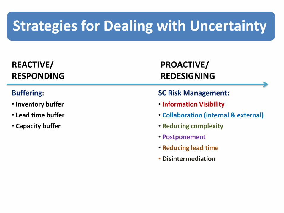
Strategies for Dealing with Uncertainty

Buffering:

• Inventory buffer

• Lead time buffer

• Capacity buffer

REACTIVE/ RESPONDING

PROACTIVE/ REDESIGNING

SC Risk Management:

• Information Visibility

• Collaboration (internal & external)

• Reducing complexity

• Postponement

• Reducing lead time

• Disintermediation

Strategy References

Information sharing Lee et al (1997), Tang (2006)

Cross-functional coordination Pujawan & Graldin (2009); Pujawan & Smart (2011);

CPFR Tang (2006)

VMI Dysney & Towill (2003); Tang (2006), Wong et al (2009)

Consolidation Thomas & Griffin (1996)

Disintermediation Lee et al 91997)

Stable pricing policy Lee et al (1997)

Reducing lead time Hayya et al (2011); Ryu & Lee (2003); Ouyang et al (2007); Glock (2011)

Reducing setup time Diaby (1995); Samaddar (2001); Coates et al 91996)

Reducing order cost Zhang et al (2007);

Safety stock, Augmentation Quantity Pujawan (2004), Pujawan & Silver (2008), Osman & Demirli (2012)

Safety lead time Molinder (1997); Chang (1985)

Freezing schedule Blackburn et al., 1985; Kadipasaoglu and Sridharan, 1995; Zhao et al., 1995;

Xie et al., 2003; Robinson et al, 2008

Increasing component commonality / Part standardization

Meixell (2005); Mohebbi & Choobineh (2005); Baud-Lavigne et al (2012)

Adding backup supplier Tang (2006)

Supplier development Shin et al (2000)

Risk pooling / inventory centralization Weng (1999); Park et al (2010); Gaur & ravindran (2006); Snyder et al

(2007)

Extra production capacity Das (2011)

Outsourcing / subcontracting Stevenson & Spring (2007)

Capacity flexibility Pujawan (2004)

Postponement Lee & Tang (1997), Tang (2006), Yang et al (2004), Gunasekaran & Ngai

(2005), Ernst & kamrad (2000); Lin & Wang (2011)

Responsiveness

Cost

Safety Stock

Stock Centralization VMI

CPFR

Cross-functional coordination

Reducing lead time

Freezing schedule

Part standardization

Supplier development

Extra capacity

Safety lead time

Increasing capacity flexibility

Disintermediation

Outsourcing

Information sharing

Postponement

Uncertainty in Transportation and Distribution

• A problem of high importance in practice, but received limited attention by the academics

– Cost related to transportation is substantial

– Complex, closed-loop system

– A great challange for countries with poor transportation infrastructure and key people work with high risks & low wages (and low morale)

Transportation Uncertainty: A closed-loop system

Demand

Uncertain delivery time

space for buffer

Transportation is a complex issue in Indonesia [over 17.000 islands, 3 time zones, population +230 millions, West-East imbalance]

Uncertainty Related to Transportation & Distribution

Loading

Shipment

Unloading

Going back

waiting

waiting

• Too many trucks/ships coming • Arrive not during working hours • No items to be loaded

• Trucks / ships are in queue • Arrive not during working hours • Full storage

• Uncertain road/sea condition • Uncertain weather condition • Uncertain truck /ship condition • Drivers make more stops than normally

• Uncertain road /sea condition • Uncertain weather condition • Uncertain vehicle/ships condition • Drivers make more stops than normally

• Uncertain unloading speed • Breakdown of equipments

• Uncertain loading speed • Breakdown of equipments

Process Analysis in Transportation: Much opportunities for improvements

Productive Time: loading, sailing, unloading

Non-Productive Time: Waiting / Queueing

40% - 60% Productive Time: loading, travelling, unloading

Non-Productive Time: Waiting / Queueing

30% - 70%

Case Study

Problems

• Destination varies substantially (could be as short as a few kilometers and as long as over 700 kilometers), but there was no attempt to segment the queue.

• Time window is not taken into account when departing trucks. Many trucks wait for the following day for unloading.

Queue time before loading, average around 4 hours

Queue time @ Plant travel Queue time @ destination Travel back 1 cycle

2,5 cycle

Proposed Solutions

• Solution 1: Queue segmentation (priority is given to short destination)

• Solution 2: Consider time window (trucks departing 24 hours, but most destinations follow normal working hours / day time only)

Express Loading for Short Destinations and Take into Account Time Windows

Normal path

Express path

Zone I between 03.00 – 10.00 Zone III for the rest of time

Zone II for night delivery Zone III for the rest of time

OBJECTIVE: minimize truck arriving between 5 pm to 6 am + minimize Q time for short distances.

Case 1: Simulation for Short Distance, Low Uncertainty

• Travel time N[7; 2] hours

• There is a probability that a truck arrives at destination within time window, but has to queue/wait until the following day. This probability is about 50% and in case of waiting, the waiting time is uniformly distributed between 0 – 8 hours.

Planning for time windows is critical for short distance

00 06.00 18.00 24.00

ON OFF OFF

00

Loading Travelling Waiting Ready for

Unload

Maximize the probability of this event falling in the green area

N (7; 2)

0 wp. 0.5

U[0 – 8] wp. 0.5

24.00

00 06 18 30 42 54 66 78 90 102

OFF OFF OFF OFF OFF ON ON ON ON

Departure U [ 03 – 10]

Results: Relatively Short Distance, Travel Time about 7 hours

Range of Departure Time

P[Arrive= Time Window]

P[Unload = Same Day]

[03.00 - 08.00] 99% 97%

[03.00 - 09.00] 97% 95%

[03.00 - 10.00] 95% 92%

[03.00 - 11.00] 93% 89%

[03.00 - 12.00] 84% 80%

[03.00 - 13.00] 77% 73%

About 27% probability that a truck has to

wait for the following day for unloading

The results on Monte Carlo simulation with sample size of 1295.

Case 2: Simulation for Long Distance, high Uncertainty

• Travel time N[85; 25] hours

• There is a probability that a truck arrives at destination within time window, but has to queue/wait until the following day. This probability is about 50% and in case of waiting, the waiting time is uniformly distributed between 0 – 8 hours.

An example of trip time distribution to a destination of about 730 km

0

5

10

15

20

25

30

35

400

10

20

30

40

50

60

70

80

90

10

0

11

0

12

0

13

0

14

0

15

0

16

0

17

0

18

0

19

0

20

0

21

0

22

0

23

0

24

0

36

5,0

7

Fre

qu

en

cy

Time interval

When travelling time is highly uncertain, planning for time windows may have no impact

00 06.00 18.00 24.00

ON OFF OFF

00

Loading Travelling Waiting Ready for

Unload

Maximize the probability of this event falling in green zone

N (85, 25)

0 wp. 0.5

U[0 – 8] wp. 0.5

24.00

00 06 18 30 42 54 66 78 90 102

OFF OFF OFF OFF OFF ON ON ON ON

Departure U [ 0 – 24]

Range of Total Time

Within Time Windows?

Arrival Time

Time Ready for Unload

[0-6] OFF 0 0

[6-18] ON 3 3

[18-30] OFF 4 1

[30-42] ON 11 12

[42-54] OFF 40 31

[54-66] ON 79 68

[66-78] OFF 151 149

[78-90] ON 199 189

[90-102] OFF 230 226

[102-114] ON 218 232

[114-126] OFF 168 166

[126-138] ON 117 127

[138-150] OFF 51 65

[150-162] ON 15 16

[162-174] OFF 9 9

Percentage OFF 50,4 50

Percentage ON 49,6 50

The results on Monte Carlo simulation with sample size of 1295.

Results: departure time interval has no effect on the probability of arriving within the time window

Range of Departure Time

Short Distance Long Distance

P[Arrive= Time Window]

P[Unload = Same Day]

P[Arrive= Time Window]

P[Unload = Same Day]

[03.00 - 08.00] 99% 97% 52% 51%

[03.00 - 09.00] 97% 95% 48% 48%

[03.00 - 10.00] 95% 92% 49% 50%

[03.00 - 11.00] 93% 89% 48% 48%

[03.00 - 12.00] 84% 80% 49% 49%

[03.00 - 13.00] 77% 73% 49% 50%

[00.00 - 24.00] 50% 50% 50% 50%

Shifting Paradigm: Reacting to Demand instead of Reacting to Order

• Orders from distributors do not reflect sales pattern (due to forecast error or speculative motives)

• This is worsen with the company’s policy to require one month frozen orders

If distributors overestimated demand, too many trucks

shipped, warehouse full, long queue, transportation cost is high

If distributors underestimated demand, shortages happened

Proposed Solution

• There is an obvious need for better information visibility (not only demand and inventory, but also truck in transit and the associated quantity, warehouse capacity, and unloading rate).

• Shifting paradigm FROM responding to order TO responding to sales / demand.

• Challenges: information accuracy and timeliness, stakeholders involvement.

Proposed Solution

Some formulae and algoritm have been developed to improve the shipment rules.

Illustrative Example

Demand/day (tons)

Lead time (days)

On-hand (tons)

in-transit (tons)

# truck in transit

Unloading speed (truk

/ hari) WHS

capacity SDR TUR SCR

D1 50 1 100 32 1 2 200 2,6 0,50 0,41

D2 20 4 80 64 2 2 200 1,8 0,25 0,32

D3 100 2 250 32 1 3 500 1,4 0,17 0,16

D4 15 0,5 60 0 0 1 100 8,0 0,00 0,53

D5 120 1 30 32 1 3 400 0,5 0,33 0,00

D6 30 0,4 40 150 1 2 100 15,8 1,25 1,78

D7 20 2 50 0 0 1 100 1,3 0,00 0,10

• High priority is given to destinations with low SDR, TUR, and SCR. • Shipment should not be made to destinations with TUR or SCR values of 1 or

higher.

Algorithm

• Step 1: Retrieve data {SO, on hand, in transit, demand, lead time, SDR Target}

For all distributors:

• Step 2: Calculate SDR, TUR, and SCR

• Step 3: Sort according to SDR in ascending order. Do NOT ship today if both TUR and SCR values are 1 or more.

• Step 4: Calculate amount of day shipment

SQ = max[0, [(SDR Target-SDR)*daily demand*lead time]

• Step 5: Calculate number of trucks needed: #Trucks = [SQ/truck capacity]

• Step 6: Aggregate # trucks needed for the day [TN]

• Step 7: Find out number of trucks available [TA]. If TA < TN, do rationalization (Each is reduced by TA/TN).

Responsiveness

Cost

Safety Stock

Stock Centralization VMI

CPFR

Cross-functional coordination

Reducing lead time

Freezing schedule

Part standardization

Supplier development

Extra capacity

Safety lead time

Increasing capacity flexibility

Disintermediation

Outsourcing

Information sharing

Postponement

Uncertainty and Supply Chain Game

Plant

TSP

DIST

End Customers

Hold trucks

High Costs

Long frozen orders

Truck drivers

Research Implications

• Transportation scheduling to improve truck utilization considering stochastic travel times and waiting time at the destination point.

• Supply chain power structure in the context of transportation different rules of the game.

• The impacts of information visibility in improving transportation and distribution decisions.

The 6th Operations and Supply Chain Management (OSCM) Conference, Bali,

10 – 12 December 2014

www.oscm-forum.org

www.oscm2014.org