Debiased Off-Policy Evaluation for Recommendation Systems

Debiased Off-Policy Evaluation for Recommendation Systems

YUSUKE NARITA, Yale University, USA

SHOTA YASUI, CyberAgent, Inc., Japan

KOHEI YATA, Yale University, USA

Efficient methods to evaluate new algorithms are critical for improving interactive bandit and reinforcement learning systems such as

recommendation systems. A/B tests are reliable, but are time- and money-consuming, and entail a risk of failure. In this paper, we

develop an alternative method, which predicts the performance of algorithms given historical data that may have been generated

by a different algorithm. Our estimator has the property that its prediction converges in probability to the true performance of a

counterfactual algorithm at a rate of

√𝑁 , as the sample size 𝑁 increases. We also show a correct way to estimate the variance of our

prediction, thus allowing the analyst to quantify the uncertainty in the prediction. These properties hold even when the analyst does

not know which among a large number of potentially important state variables are actually important. We validate our method by a

simulation experiment about reinforcement learning. We finally apply it to improve advertisement design by a major advertisement

company. We find that our method produces smaller mean squared errors than state-of-the-art methods.

CCS Concepts: • Information systems → Online advertising; • Computing methodologies → Learning from implicit feed-back.

Additional Key Words and Phrases: ad design, off-policy evaluation, bandit, reinforcement learning

ACM Reference Format:Yusuke Narita, Shota Yasui, and Kohei Yata. 2021. Debiased Off-Policy Evaluation for Recommendation Systems. In Fifteenth ACM

Conference on Recommender Systems (RecSys ’21), September 27-October 1, 2021, Amsterdam, Netherlands. ACM, New York, NY, USA,

8 pages. https://doi.org/10.1145/3460231.3474231

1 INTRODUCTION

Interactive bandit and reinforcement learning (RL) systems (e.g., ad/news/recommendation/search platforms, personal-

ized education and medicine) produce log data valuable for evaluating and redesigning the systems. For example, the

logs of a news recommendation system record which news article was presented and whether the user read it, giving

the system designer a chance to make its recommendation more relevant [11].

Exploiting log data is, however, more difficult than conventional supervised machine learning: the result of each log

is only observed for the action chosen by the system (e.g., the presented news) but not for all the other actions the

system could have taken. Moreover, the log entries are biased in that the logs over-represent actions favored by the

system.

A potential solution to this problem is an A/B test that compares the performance of counterfactual systems. However,

A/B testing counterfactual systems is often technically or managerially infeasible, since deploying a new policy is time-

and money-consuming, and entails a risk of failure.

This leads us to the problem of counterfactual (off-policy, offline) evaluation, where one aims to use batch data collected

by a logging policy to estimate the value of a counterfactual policy or algorithm without deploying it. Such evaluation

allows us to compare the performance of counterfactual policies to decide which policy should be deployed in the field.

This alternative approach thus solves the above problem with the naive A/B test approach. Key prior studies include

© 2021 Copyright held by the owner/author(s). Publication rights licensed to ACM.

Manuscript submitted to ACM

1

arX

iv:2

002.

0853

6v3

[cs

.LG

] 2

Aug

202

1

https://doi.org/10.1145/3460231.3474231

RecSys ’21, September 27-October 1, 2021, Amsterdam, Netherlands Yusuke Narita, Shota Yasui, and Kohei Yata

Dudík et al. [4], Gilotte et al. [6], Li et al. [11, 12], Narita et al. [14], Strehl et al. [19], Swaminathan et al. [20], Wang

et al. [24] for bandit algorithms, and Farajtabar et al. [5], Irpan et al. [7], Jiang and Li [8], Kallus and Uehara [9], Liu

et al. [13], Precup et al. [17], Thomas and Brunskill [21], Uehara et al. [23] for RL algorithms.

Method. For off-policy evaluation with log data of RL feedback, this paper develops and empirically implements

a novel technique with desirable theoretical properties. To do so, we consider a class of RL algorithms, including

contextual bandit algorithms as important special cases. This class includes most of the widely-used algorithms such as

(deep) Q-learning, Actor Critic, contextual 𝜖-greedy, and Thompson Sampling, as well as their non-contextual analogs

and random A/B testing. We allow the logging policy to be an unknown function of numerous potentially important

state variables. This feature is salient in real-world applications. We also allow the evaluation target policy to be

degenerate, again a key feature of real-life situations.

We consider an offline estimator for the expected reward from a counterfactual policy. Our estimator integrates a

well-known Doubly Robust estimator ([18] and modern studies cited above) with “Double/Debiased Machine Learning”

developed in econometrics and statistics [2, 3]. Building upon these prior studies, we show that our estimator is

“

√𝑁 -consistent” in the sense that its prediction converges in probability to the true performance of a counterfactual

policy at a rate of 1/√𝑁 as the sample size 𝑁 increases. Our estimator is also shown to be “asymptotically normal,”

meaning that it has an approximately normal distribution as 𝑁 gets large. We also provide a consistent estimator of

its asymptotic variance, thus allowing for the measurement of statistical uncertainty in our prediction. Moreover, for

special cases in which data are generated by contextual bandit algorithms, our estimator has the lowest variance in a

wide class of estimators, achieving variance reduction relative to standard estimators. Importantly, these properties

hold even when the analyst does not know which among a large number of potentially important state variables are

actually important.

Simulation Experiment. We evaluate the performance of our estimator by conducting an experiment in a slightly

different version of the OpenAI Gym CartPole-v0 environment [1]. In this version, there are many more state variables

than the original one and some of them are irrelevant to the reward. In this challenging environment, our estimator

produces smaller mean squared errors than widely-used benchmark methods (Doubly Robust estimator in the spirit of

Jiang and Li [8] and Thomas and Brunskill [21] and Inverse Probability Weighting estimator).

Real-World Experiment. We empirically apply our estimator to evaluate and optimize the design of online

advertisement formats. Our application is based on proprietary data provided by CyberAgent Inc., the second largest

Japanese advertisement company with about 5 billion USD market capitalization (as of February 2020). This company

uses randomly chosen bandit algorithms to determine the visual design of advertisements assigned to users. This A/B

test of randomly choosing an algorithm produces logged data and the ground truth for the performance of alternative

algorithms. We use this data to examine the performance of our proposed method. We use the log data from an algorithm

to predict the click through rates (CTR) of another algorithm, and assess the accuracy of our prediction by comparing it

with the ground truth. This exercise shows that our estimator produces smaller mean squared errors than widely-used

benchmark methods (Doubly Robust estimator in the spirit of Dudík et al. [4] and Inverse Probability Weighting

estimator). This improvement is statistically significant at the 5% level. Importantly, this result holds regardless of

whether we know the data-generating logging policy or not, which shows that our estimator can substantially reduce

bias and uncertainty we face in real-world decision-making.

This improved performance motivates us to use our estimator to optimize the advertisement design for maximizing

the CTR. We estimate how much the CTR would be improved by a counterfactual policy of choosing the best action

(advertisement) for each context (user characteristics). This exercise produces the following bottom line: Our estimator

2

Debiased Off-Policy Evaluation for Recommendation Systems RecSys ’21, September 27-October 1, 2021, Amsterdam, Netherlands

predicts the hypothetical policy to statistically significantly improve the CTR by 30% (compared to the logging policy)

in one of the three campaigns we analyze. Our approach thus generates valuable managerial conclusions.

2 SETUP

2.1 Data Generating Process

We consider historical data from a Markov Decision Process (MDP) as a mathematical description of RL and bandit

algorithms. An MDP is given by M = ⟨S,A, 𝑃𝑆0, 𝑃𝑆 , 𝑃𝑅⟩, where S is the state space, A is the action space, 𝑃𝑆0

: S →[0, 1] is the initial state distribution, 𝑃𝑆 : S ×A → Δ(S) is the transition function with 𝑃𝑆 (𝑠 ′ |𝑠, 𝑎) being the probabilityof seeing state 𝑠 ′ after taking action 𝑎 given state 𝑠 , and 𝑃𝑅 : S × A × R→ [0, 1] be the conditional distribution of the

immediate reward with 𝑃𝑅 (·|𝑠, 𝑎) being the immediate reward distribution conditional on the state and action being

(𝑠, 𝑎). We assume that the state and action spaces S and A are finite. Given 𝑃𝑅 , we define the mean reward function

` : S × A → R as ` (𝑠, 𝑎) =∫𝑟𝑑𝑃𝑅 (𝑟 |𝑠, 𝑎).

We call a function 𝜋 : S → Δ(A) a policy, which assigns each state 𝑠 ∈ S a distribution over actions, where 𝜋 (𝑎 |𝑠)is the probability of taking action 𝑎 when the state is 𝑠 . Let 𝐻 = (𝑆0, 𝐴0, 𝑅0, ..., 𝑆𝑇 , 𝐴𝑇 , 𝑅𝑇 ) be a trajectory, where 𝑆𝑡 , 𝐴𝑡 ,and 𝑅𝑡 are the state, the action, and the reward in step 𝑡 , respectively, and 𝑇 denotes the last step and is fixed. We say

that a trajectory 𝐻 is generated by a policy 𝜋 , or 𝐻 ∼ 𝜋 in short if 𝐻 is generated by repeating the following process for

𝑡 = 0, ...,𝑇 : (1) When 𝑡 = 0, the state 𝑆𝑡 is drawn from the initial distribution 𝑃𝑆0. When 𝑡 ≥ 1, 𝑆𝑡 is determined based on

the transition function 𝑃𝑆 (·|𝑆𝑡−1, 𝐴𝑡−1). (2) Given 𝑆𝑡 , the action 𝐴𝑡 is randomly chosen based on 𝜋 (·|𝑆𝑡 ). (3) The reward𝑅𝑡 is drawn from the conditional reward distribution 𝑃𝑅 (·|𝑆𝑡 , 𝐴𝑡 ).

Suppose that we observe historical data {𝐻𝑖 }𝑁𝑖=1where trajectories are independently generated by a fixed behavior

policy 𝜋𝑏 , i.e., 𝐻𝑖 ∼ 𝜋𝑏 independently across 𝑖 . The historical data is a collection of i.i.d. trajectories. Importantly, we

allow the components of the data generating processM and 𝜋𝑏 to vary with the sample size 𝑁 . Specifically, letM𝑁

and 𝜋𝑏𝑁 be the MDP and the behavior policy, respectively, when the sample size is 𝑁 , and let P𝑁 denote the resulting

probability distribution of 𝐻𝑖 . P𝑁 is allowed to vary with 𝑁 in a way that the functions 𝑃𝑆0𝑁 , 𝑃𝑅𝑁 and 𝜋𝑏𝑁 are high

dimensional relative to sample size 𝑁 even when 𝑁 is large. In some RL problems, for example, there are a large number

of possible states. To capture the feature that the number of states |S𝑁 | is potentially large relative to sample size 𝑁 ,

we may consider a sequence of P𝑁 such that |S𝑁 | is increasing with 𝑁 . For the sake of notational simplicity, we make

implicit the dependence ofM and 𝜋𝑏 on 𝑁 .

We assume that we know the state space S and the action space A but know none of the functions 𝑃𝑆0, 𝑃𝑆 and 𝑃𝑅 .

In some environments, we know the function 𝜋𝑏 or observe the probability vector (𝜋𝑏 (𝑎 |𝑆𝑖𝑡 ))𝑎∈A,𝑡=0,...,𝑇 for every

trajectory 𝑖 in the historical data. Our approach is usable regardless of the availability of such knowledge on the behavior

policy.

2.2 Prediction Target

With the historical data {𝐻𝑖 }𝑁𝑖=1, we are interested in estimating the discounted value of the evaluation policy 𝜋𝑒 , which

might be different from 𝜋𝑏 : with 𝛾 ∈ [0, 1] as the discount factor,

𝑉 𝜋𝑒 B E𝐻∼𝜋𝑒

[𝑇∑︁𝑡=0

𝛾𝑡𝑅𝑡

].

3


3 ESTIMATOR AND ITS PROPERTIES

The estimation of 𝑉 𝜋𝑒 involves estimation of the behavior policy 𝜋𝑏 (if unknown), the transition function 𝑃𝑆 , and the

mean reward function `. These functions may be high dimensional in the sense of having a large number of arguments,

possibly much larger than the number of trajectories 𝑁 . To handle the issue, we use Double/Debiased Machine Learning

(DML) by Chernozhukov et al. [2]. DML is a general method for estimation and inference of semiparametric models in

the presence of a high-dimensional vector of control variables, and is characterized by two key features, cross-fitting

and Neyman orthogonality, which we will discuss in detail later. These two features play a role in reducing the bias

that may arise due to the estimation of high-dimensional parameters, which makes DML suitable for the off-policy

evaluation problem with potentially high dimensions of 𝜋𝑏 , 𝑃𝑆 and `.

Before presenting our estimator, we introduce some notation. 𝐻𝑠,𝑎𝑡 = (𝑆0, 𝐴0, ..., 𝑆𝑡 , 𝐴𝑡 ) is a trajectory of the state

and action up to step 𝑡 . 𝜌𝜋𝑒𝑡 : (S × A)𝑡+1 → R+ is the importance weight function:

𝜌𝜋𝑒𝑡 (𝐻𝑠,𝑎𝑡 ) B

𝑡∏𝑡 ′=0

𝜋𝑒 (𝐴𝑡 ′ |𝑆𝑡 ′)𝜋𝑏 (𝐴𝑡 ′ |𝑆𝑡 ′)

. (1)

This equals the probability of 𝐻 up to step 𝑡 under the evaluation policy 𝜋𝑒 divided by its probability under the behavior

policy 𝜋𝑏 . Viewing 𝜌𝜋𝑒𝑡 as a function of 𝜋𝑏 , define 𝜌

𝜋𝑒𝑡 (𝐻𝑠,𝑎𝑡 ; �̃�𝑏 ) as the value of 𝜌𝜋𝑒𝑡 (𝐻𝑠,𝑎𝑡 ) with the true behavior policy

𝜋𝑏 replaced with a candidate function �̃�𝑏 :

𝜌𝜋𝑒𝑡 (𝐻𝑠,𝑎𝑡 ; �̃�𝑏 ) B

𝑡∏𝑡 ′=0

𝜋𝑒 (𝐴𝑡 ′ |𝑆𝑡 ′)�̃�𝑏 (𝐴𝑡 ′ |𝑆𝑡 ′)

.

We can think of 𝜌𝜋𝑒𝑡 (𝐻𝑠,𝑎𝑡 ; �̃�𝑏 ) as the estimated importance weight function when we use �̃�𝑏 as the estimate of 𝜋𝑏 .

By definition, 𝜌𝜋𝑒𝑡 (𝐻𝑠,𝑎𝑡 ;𝜋𝑏 ) = 𝜌

𝜋𝑒𝑡 (𝐻𝑠,𝑎𝑡 ), where the left-hand side is 𝜌

𝜋𝑒𝑡 (𝐻𝑠,𝑎𝑡 ; �̃�𝑏 ) evaluated at the true 𝜋𝑏 and the

right-hand side is the true importance weight function. Finally, let 𝑞𝜋𝑒𝑡 : S × A → R be the state-action value function

under policy 𝜋𝑒 at step 𝑡 , where 𝑞𝜋𝑒𝑡 (𝑠, 𝑎) B E𝐻∼𝜋𝑒 [

∑𝑇𝑡 ′=𝑡 𝛾

𝑡 ′−𝑡𝑅𝑡 ′ |𝑆𝑡 = 𝑠, 𝐴𝑡 = 𝑎]. Using 𝑃𝑆 , ` and 𝜋𝑒 , 𝑞𝜋𝑒𝑡 can be

obtained recursively: let

𝑞𝜋𝑒𝑇

(𝑠, 𝑎) = ` (𝑠, 𝑎) (2)

and for 𝑡 = 0, ...,𝑇 − 1,

𝑞𝜋𝑒𝑡 (𝑠, 𝑎) = ` (𝑠, 𝑎) + 𝛾

∑︁(𝑠′,𝑎′)

𝑃𝑆 (𝑠 ′ |𝑠, 𝑎)𝜋𝑒 (𝑎′ |𝑠 ′)𝑞𝜋𝑒𝑡+1(𝑠 ′, 𝑎′) . (3)

Our estimator is based on the following expression of 𝑉 𝜋𝑒 [21]:

𝑉 𝜋𝑒 = E𝐻∼𝜋𝑏[𝜓 (𝐻 ;𝜋𝑏 , {𝑞𝜋𝑒𝑡 }𝑇𝑡=0

)], (4)

where for any candidate tuple [̃ = (�̃�𝑏 , {𝑞𝜋𝑒𝑡 }𝑇𝑡=0

), we define

𝜓 (𝐻 ; [̃) =𝑇∑︁𝑡=0

𝛾𝑡{𝜌𝜋𝑒𝑡 (𝐻𝑠,𝑎𝑡 ; �̃�𝑏 ) (𝑅𝑡 − 𝑞𝜋𝑒𝑡 (𝑆𝑡 , 𝐴𝑡 ))+𝜌𝜋𝑒𝑡−1

(𝐻𝑠,𝑎𝑡−1

; �̃�𝑏 )∑︁𝑎∈A

𝜋𝑒 (𝑎 |𝑆𝑡 )𝑞𝜋𝑒𝑡 (𝑆𝑡 , 𝑎)}, (5)

where 𝜌𝜋𝑒−1

= 1. To give an intuition behind the expression, we arrange the terms as follows:

𝜓 (𝐻 ; [̃) =𝑇∑︁𝑡=0

𝛾𝑡 𝜌𝜋𝑒𝑡 (𝐻𝑠,𝑎𝑡 ; �̃�𝑏 )𝑅𝑡 +

𝑇∑︁𝑡=0

𝛾𝑡{−𝜌𝜋𝑒𝑡 (𝐻𝑠,𝑎𝑡 ; �̃�𝑏 )𝑞𝜋𝑒𝑡 (𝑆𝑡 , 𝐴𝑡 ) + 𝜌𝜋𝑒𝑡−1


; �̃�𝑏 )∑︁𝑎∈A

𝜋𝑒 (𝑎 |𝑆𝑡 )𝑞𝜋𝑒𝑡 (𝑆𝑡 , 𝑎)}.

4


The first term is the well-known Inverse Probability Weighting (IPW) estimator. The second term serves as a control

variate that has zero mean as long as we plug in the true 𝜋𝑏 ; the mean of the term remains zero regardless of the function

we plug in for {𝑞𝜋𝑒𝑡 }𝑇𝑡=0

. This is the key to make our estimator insensitive to {𝑞𝜋𝑒𝑡 }𝑇𝑡=0

. We construct our estimator as

follows.

(1) Take a𝐾-fold random partition (𝐼𝑘 )𝐾𝑘=1of trajectory indices {1, ..., 𝑁 } such that the size of each fold 𝐼𝑘 is 𝑛 = 𝑁 /𝐾 .

Also, for each 𝑘 = 1, ..., 𝐾 , define 𝐼𝑐𝑘B {1, ..., 𝑁 } \ 𝐼𝑘 .

(2) For each 𝑘 = 1, ..., 𝐾 , construct estimators 𝜋𝑏,𝑘 (if 𝜋𝑏 is unknown), ˆ̀𝑘 and 𝑃𝑆,𝑘 of 𝜋𝑏 , ` and 𝑃𝑆 using the subset

of data {𝐻𝑖 }𝑖∈𝐼𝑐𝑘. We then construct estimator {𝑞𝜋𝑒

𝑡,𝑘}𝑇𝑡=0

of {𝑞𝜋𝑒𝑡 }𝑇𝑡=0

by plugging ˆ̀𝑘 and 𝑃𝑆,𝑘 into the recursive

formulation (2) and (3).

(3) Given [̂𝑘 = (𝜋𝑏,𝑘 , {𝑞𝜋𝑒𝑡,𝑘 }𝑇𝑡=0

), 𝑘 = 1, ..., 𝐾 , the DML estimator 𝑉𝜋𝑒DML

is given by

𝑉𝜋𝑒DML

=1

𝐾

𝐾∑︁𝑘=1

1

𝑛

∑︁𝑖∈𝐼𝑘

𝜓 (𝐻𝑖 ; [̂𝑘 )

=1

𝐾

𝐾∑︁𝑘=1

1

𝑛


𝑇∑︁𝑡=0

𝛾𝑡{𝜌𝜋𝑒𝑡 (𝐻𝑠,𝑎

𝑖𝑡;𝜋𝑏,𝑘 ) (𝑅𝑖𝑡 − 𝑞𝜋𝑒𝑡,𝑘 (𝑆𝑖𝑡 , 𝐴𝑖𝑡 )) + 𝜌

𝜋𝑒𝑡−1

(𝐻𝑠,𝑎𝑖𝑡−1

;𝜋𝑏,𝑘 )∑︁𝑎∈A

𝜋𝑒 (𝑎 |𝑆𝑖𝑡 )𝑞𝜋𝑒𝑡,𝑘 (𝑆𝑖𝑡 , 𝑎)}.

Possible estimation methods for 𝜋𝑏 , ` and 𝑃𝑆 in Step 2 are (i) classical nonparametric methods such as kernel and

series estimation, (ii) off-the-shelf machine learning methods such as random forests, lasso, neural nets, and boosted

regression trees, and (iii) existing methods developed in the off-policy policy evaluation literature such as representation

balancing MDPs [13]. These methods, especially (ii) and (iii), are usable even when the analyst does not know which

among a large number of potentially important state variables are actually important. This DML estimator differs from

the Doubly Robust (DR) estimator developed by Jiang and Li [8] and Thomas and Brunskill [21] in that we use the

cross-fitting procedure, as explained next.

A. Cross-Fitting. The above method uses a sample-splitting procedure called cross-fitting, where we split the data

into 𝐾 folds, take the sample analogue of Eq. (4) using one of the folds (𝐼𝑘 ) with 𝜋𝑏 and {𝑞𝜋𝑒𝑡 }𝑇𝑡=0

estimated from the

remaining folds (𝐼𝑐𝑘) plugged in, and average the estimates over the 𝐾 folds to produce a single estimator. Cross-fitting

has two advantages. First, if we use instead the whole sample both for estimating 𝜋𝑏 and {𝑞𝜋𝑒𝑡 }𝑇𝑡=0

and for computing the

final estimate of 𝑉 𝜋𝑒 (the “full-data” variant of the DR estimator of Thomas and Brunskill [21]), substantial bias might

arise due to overfitting [2, 15]. Cross-fitting removes the potential bias by making the estimate of 𝑉 𝜋𝑒 independent of

the estimates of 𝜋𝑏 and {𝑞𝜋𝑒𝑡 }𝑇𝑡=0

.

Second, a standard sample splitting procedure uses a half of the data to construct estimates of 𝜋𝑏 and {𝑞𝜋𝑒𝑡 }𝑇𝑡=0

and

the other half to compute the estimate of 𝑉 𝜋𝑒 (the DR estimator of Jiang and Li [8] and the “half-data” variant of the

DR estimator of Thomas and Brunskill [21]). In contrast, cross-fitting swaps the roles of the main fold (𝐼𝑘 ) and the rest

(𝐼𝑐𝑘) so that all trajectories are used for the final estimate, which enables us to make efficient use of data.

B. Neyman Orthogonality. There is another key ingredient important for DML to have desirable properties. The

DML estimator is constructed by plugging in the estimates of 𝜋𝑏 and {𝑞𝜋𝑒𝑡 }𝑇𝑡=0

, which may be biased due to regularization

if they are estimated with machine learning methods. However, the DML estimator is robust to the bias, since𝜓 satisfies

the Neyman orthogonality condition [2]. The condition requires that for any candidate tuple [̃ = (�̃�𝑏 , {𝑞𝜋𝑒𝑡 }𝑇𝑡=0

),

𝜕E𝐻∼𝜋𝑏 [𝜓 (𝐻 ;[ + 𝑟 ([̃ − [))]𝜕𝑟

��𝑟=0

= 0,

5


where [ = (𝜋𝑏 , {𝑞𝜋𝑒𝑡 }𝑇𝑡=0

) is the tuple of the true functions (see Appendix E for the proof that DML satisfies this).

Intuitively, the Neyman orthogonality condition means that the right-hand side of Eq. (4) is locally insensitive to the

value of 𝜋𝑏 and {𝑞𝜋𝑒𝑡 }𝑇𝑡=0

. More formally, the first-order approximation of the bias caused by using [̃ instead of the true

[ is given by

E𝐻∼𝜋𝑏 [𝜓 (𝐻 ; [̃))] − E𝐻∼𝜋𝑏 [𝜓 (𝐻 ;[)] ≈𝜕E𝐻∼𝜋𝑏 [𝜓 (𝐻 ;[ + 𝑟 ([̃ − [))]

𝜕𝑟

��𝑟=0

,

which is exactly zero by the Neyman orthogonality condition. As a result, plugging in noisy estimates of 𝜋𝑏 and {𝑞𝜋𝑒𝑡 }𝑇𝑡=0

does not strongly affect the estimate of 𝑉 𝜋𝑒 .

In contrast, IPW is based on the following expression of 𝑉 𝜋𝑒 : 𝑉 𝜋𝑒 = E𝐻∼𝜋𝑏 [𝜓IPW (𝐻 ;𝜋𝑏 )], where for any candidate

�̃�𝑏 , we define

𝜓IPW (𝐻 ; �̃�𝑏 ) =𝑇∑︁𝑡=0

𝛾𝑡 𝜌𝜋𝑒𝑡 (𝐻𝑠,𝑎𝑡 ; �̃�𝑏 )𝑅𝑡 . (6)

The Neyman orthogonality condition does not hold for IPW: for some �̃�𝑏 ≠ 𝜋𝑏 ,𝜕E𝐻∼𝜋𝑏 [𝜓IPW (𝐻 ;𝜋𝑏+𝑟 (�̃�𝑏−𝜋𝑏 )) ]

𝜕𝑟

��𝑟=0

≠ 0.

Therefore, IPW is not robust to the bias in the estimate of 𝜋𝑏 .

3.1√𝑁 -consistency and Asymptotic Normality

Let 𝜎2 = E𝐻∼𝜋𝑏 [(𝜓 (𝐻 ;[) −𝑉 𝜋𝑒 )2] be the variance of𝜓 (𝐻 ;[). To derive the properties of the DML estimator, we make

the following assumption.

Assumption 1. (a) There exists a constant 𝑐0 > 0 such that 𝑐0 ≤ 𝜎2 < ∞ for all 𝑁 .

(b) For each 𝑘 = 1, ..., 𝐾 , the estimator [̂𝑘 = (𝜋𝑏,𝑘 , {𝑞𝜋𝑒𝑡,𝑘 }𝑇𝑡=0

) belongs to a set T𝑁 with probability approaching one,

where T𝑁 contains the true [ = (𝜋𝑏 , {𝑞𝜋𝑒𝑡 }𝑇𝑡=0

) and satisfies the following:(i) There exist constants 𝑞 > 2 and 𝑐1 > 0 such that

sup

[̃∈T𝑁

(E𝐻∼𝜋𝑏 [(𝜓 (𝐻 ; [̃) −𝑉 𝜋𝑒 )𝑞]

)1/𝑞 ≤ 𝑐1

for all 𝑁 .

(ii) sup[̃∈T𝑁(E𝐻∼𝜋𝑏 [(𝜓 (𝐻 ; [̃) −𝜓 (𝐻 ;[))2]

)1/2

= 𝑜 (1).

(iii) sup𝑟 ∈(0,1),[̃∈T𝑁

�� 𝜕2E𝐻∼𝜋𝑏 [𝜓 (𝐻 ;[+𝑟 ([̃−[)) ]𝜕𝑟 2

�� = 𝑜 (1/√𝑁 ) .

Assumption 1 (a) assumes that the variance of 𝜓 (𝐻 ;[) is nonzero and finite. Assumption 1 (b) states that the

estimator (𝜋𝑏,𝑘 , {𝑞𝜋𝑒𝑡,𝑘 }𝑇𝑡=0

) belongs to the set T𝑁 , a shrinking neighborhood of the true (𝜋𝑏 , {𝑞𝜋𝑒𝑡 }𝑇𝑡=0

), with probability

approaching one. It requires that (𝜋𝑏,𝑘 , {𝑞𝜋𝑒𝑡,𝑘 }𝑇𝑡=0

) converge to (𝜋𝑏 , {𝑞𝜋𝑒𝑡 }𝑇𝑡=0

) at a sufficiently fast rate so that the rate

conditions in Assumption 1 (b) are satisfied.

The following proposition establishes the

√𝑁 -consistency and asymptotic normality of 𝑉

𝜋𝑒DML

and provides a

consistent estimator for the asymptotic variance. Below, ⇝ denotes convergence in distribution, and

𝑝→ denotes

convergence in probability.

Proposition 1. If Assumption 1 holds, then√𝑁𝜎−1 (𝑉 𝜋𝑒

DML−𝑉 𝜋𝑒 ) ⇝ 𝑁 (0, 1) and �̂�2 − 𝜎2

𝑝→ 0,

6


where �̂�2 = 1

𝐾

∑𝐾𝑘=1

1

𝑛

∑𝑖∈𝐼𝑘 (𝜓 (𝐻𝑖 ; [̂𝑘 ) −𝑉

𝜋𝑒DML

)2 is a sample analogue of 𝜎2.

The proof is an application of Theorems 3.1 and 3.2 of Chernozhukov et al. [2], found in Appendix E. The above

convergence result holds under any sequence of probability distributions {P𝑁 }𝑁 ≥1 as long as Assumption 1 holds.

Therefore, our approach is usable, for example, in the case where there are a growing number of possible states, that is,

|S| is increasing with 𝑁 .

Remark 1. It is possible to show that, if we impose an additional condition about the class of estimators of 𝜋𝑏 and

{𝑞𝜋𝑒𝑡 }𝑇𝑡=0

, the “full-data” variant of the DR estimator (the one that uses the whole sample both for estimating 𝜋𝑏 and


and for computing the estimate of 𝑉 𝜋𝑒 ) has the same convergence properties as our estimator [9, Theorems 6

& 8]. Cross-fitting enables us to prove the desirable properties under milder conditions than those necessary without

sample splitting.

Remark 2. For the “half-data” variant of the DR estimator (the one that uses a half of the data to estimate 𝜋𝑏 and


and the other half to compute the estimate of 𝑉 𝜋𝑒 ), a version of Proposition 1 in which

√𝑁 is replaced with√︁

𝑁 /2 holds, since this method only uses a half of the data to construct the final estimate. This reduction in the data

size leads to the variance of this estimator being roughly twice as large as that of the DML estimator, which formalizes

the efficiency of our method.

3.2 Contextual Bandits as A Special Case

When 𝑇 = 0, a trajectory takes the form of 𝐻 = (𝑆0, 𝐴0, 𝑅0). Regarding 𝑆0 as a context, it is possible to consider {𝐻𝑖 }𝑁𝑖=1

as batch data generated by a contextual bandit algorithm. In this case, the DML estimator becomes

𝑉𝜋𝑒DML

=1

𝐾

𝐾∑︁𝑘=1

1

𝑛


{ 𝜋𝑒 (𝐴𝑖0 |𝑆𝑖0)𝜋𝑏,𝑘 (𝐴𝑖0 |𝑆𝑖0)

(𝑅𝑖0 − ˆ̀𝑘 (𝑆𝑖0, 𝐴𝑖0)) +∑︁𝑎∈A

𝜋𝑒 (𝑎 |𝑆𝑖0) ˆ̀𝑘 (𝑆𝑖0, 𝑎)},

where (𝜋𝑏,𝑘 , ˆ̀𝑘 ) is the estimator of (𝜋𝑏 , `) using the subset of data {𝐻𝑖 }𝑖∈𝐼𝑐𝑘. This estimator is the same as the DR

estimator of Dudík et al. [4] except that we use the cross fitting procedure. Proposition 1 has the following implication

for the contextual bandit case. Let 𝜎2

𝑅(𝑠, 𝑎) =

∫(𝑟 − ` (𝑠, 𝑎))2𝑑𝑃𝑅 (𝑟 |𝑠, 𝑎).

Corollary 1. Suppose that 𝑇 = 0 and that Assumption 1 holds. Then,√𝑁𝜎−1

𝐶𝐵 (𝑉𝜋𝑒DML

−𝑉 𝜋𝑒 ) ⇝ 𝑁 (0, 1),

where

𝜎2

𝐶𝐵 = E𝑆0∼𝑃𝑆0

[ ∑︁𝑎∈A

𝜋𝑒 (𝑎 |𝑆0)2

𝜋𝑏 (𝑎 |𝑆0)𝜎2

𝑅 (𝑆0, 𝑎) +( ∑︁𝑎∈A

𝜋𝑒 (𝑎 |𝑆0)` (𝑆0, 𝑎) −𝑉 𝜋𝑒)

2].

The variance expression coincides with the “semiparametric efficiency bound” obtained by Narita et al. [14], where the

semiparametric efficiency bound is the smallest possible asymptotic variance among all consistent and asymptotically

normal estimators. Hence 𝑉 𝜋DML

is the lowest variance estimator.

4 EXPERIMENTS

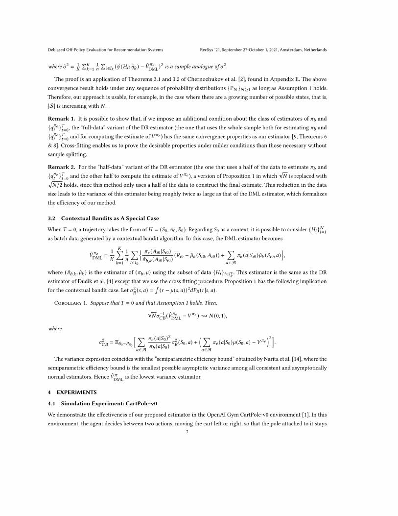
4.1 Simulation Experiment: CartPole-v0

We demonstrate the effectiveness of our proposed estimator in the OpenAI Gym CartPole-v0 environment [1]. In this

environment, the agent decides between two actions, moving the cart left or right, so that the pole attached to it stays

7


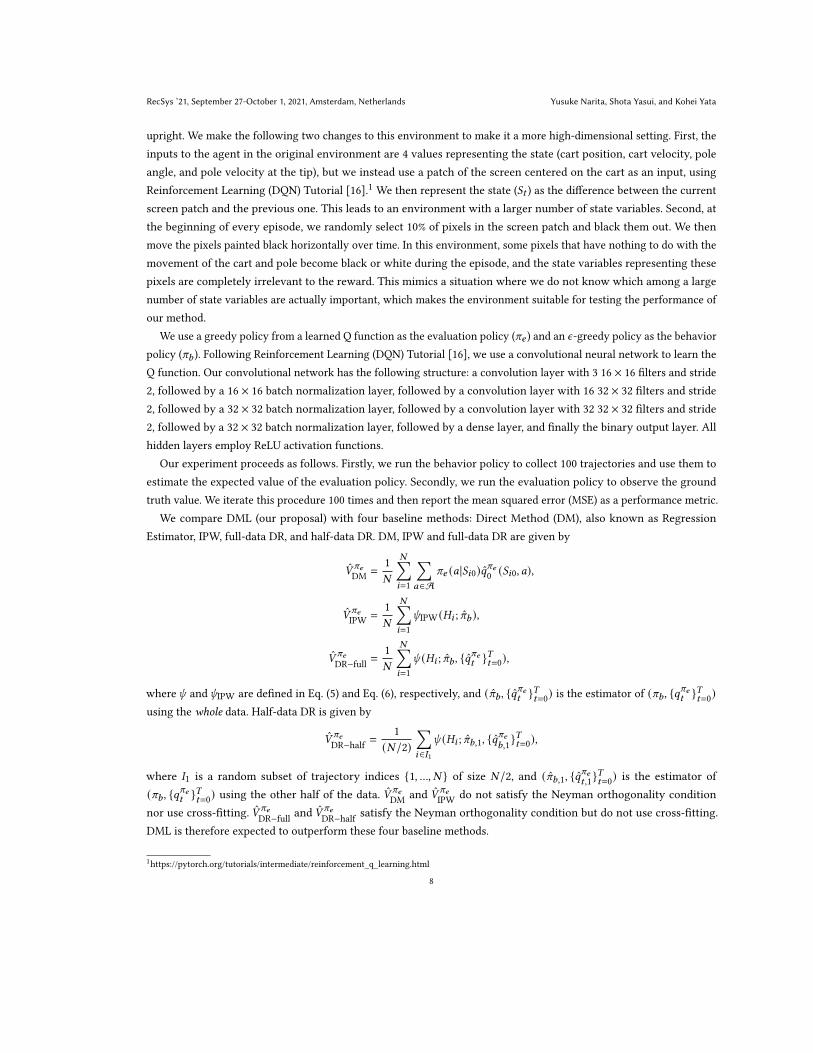
upright. We make the following two changes to this environment to make it a more high-dimensional setting. First, the

inputs to the agent in the original environment are 4 values representing the state (cart position, cart velocity, pole

angle, and pole velocity at the tip), but we instead use a patch of the screen centered on the cart as an input, using

Reinforcement Learning (DQN) Tutorial [16].1We then represent the state (𝑆𝑡 ) as the difference between the current

screen patch and the previous one. This leads to an environment with a larger number of state variables. Second, at

the beginning of every episode, we randomly select 10% of pixels in the screen patch and black them out. We then

move the pixels painted black horizontally over time. In this environment, some pixels that have nothing to do with the

movement of the cart and pole become black or white during the episode, and the state variables representing these

pixels are completely irrelevant to the reward. This mimics a situation where we do not know which among a large

number of state variables are actually important, which makes the environment suitable for testing the performance of

our method.

We use a greedy policy from a learned Q function as the evaluation policy (𝜋𝑒 ) and an 𝜖-greedy policy as the behavior

policy (𝜋𝑏 ). Following Reinforcement Learning (DQN) Tutorial [16], we use a convolutional neural network to learn the

Q function. Our convolutional network has the following structure: a convolution layer with 3 16 × 16 filters and stride

2, followed by a 16 × 16 batch normalization layer, followed by a convolution layer with 16 32 × 32 filters and stride

2, followed by a 32 × 32 batch normalization layer, followed by a convolution layer with 32 32 × 32 filters and stride

2, followed by a 32 × 32 batch normalization layer, followed by a dense layer, and finally the binary output layer. All

hidden layers employ ReLU activation functions.

Our experiment proceeds as follows. Firstly, we run the behavior policy to collect 100 trajectories and use them to

estimate the expected value of the evaluation policy. Secondly, we run the evaluation policy to observe the ground

truth value. We iterate this procedure 100 times and then report the mean squared error (MSE) as a performance metric.

We compare DML (our proposal) with four baseline methods: Direct Method (DM), also known as Regression

Estimator, IPW, full-data DR, and half-data DR. DM, IPW and full-data DR are given by

𝑉𝜋𝑒DM

=1

𝑁

𝑁∑︁𝑖=1

∑︁𝑎∈A

𝜋𝑒 (𝑎 |𝑆𝑖0)𝑞𝜋𝑒0(𝑆𝑖0, 𝑎),

𝑉𝜋𝑒IPW

=1

𝑁

𝑁∑︁𝑖=1

𝜓IPW (𝐻𝑖 ;𝜋𝑏 ),

𝑉𝜋𝑒DR−full

=1

𝑁

𝑁∑︁𝑖=1

𝜓 (𝐻𝑖 ;𝜋𝑏 , {𝑞𝜋𝑒𝑡 }𝑇𝑡=0),

where𝜓 and𝜓IPW are defined in Eq. (5) and Eq. (6), respectively, and (𝜋𝑏 , {𝑞𝜋𝑒𝑡 }𝑇𝑡=0

) is the estimator of (𝜋𝑏 , {𝑞𝜋𝑒𝑡 }𝑇𝑡=0

)using the whole data. Half-data DR is given by

𝑉𝜋𝑒DR−half

=1

(𝑁 /2)∑︁𝑖∈𝐼1

𝜓 (𝐻𝑖 ;𝜋𝑏,1, {𝑞𝜋𝑒𝑏,1}𝑇𝑡=0

),

where 𝐼1 is a random subset of trajectory indices {1, ..., 𝑁 } of size 𝑁 /2, and (𝜋𝑏,1, {𝑞𝜋𝑒𝑡,1}𝑇𝑡=0

) is the estimator of

(𝜋𝑏 , {𝑞𝜋𝑒𝑡 }𝑇𝑡=0

) using the other half of the data. 𝑉𝜋𝑒DM

and 𝑉𝜋𝑒IPW

do not satisfy the Neyman orthogonality condition

nor use cross-fitting. 𝑉𝜋𝑒DR−full

and 𝑉𝜋𝑒DR−half

satisfy the Neyman orthogonality condition but do not use cross-fitting.

DML is therefore expected to outperform these four baseline methods.

1https://pytorch.org/tutorials/intermediate/reinforcement_q_learning.html

8

https://pytorch.org/tutorials/intermediate/reinforcement_q_learning.html


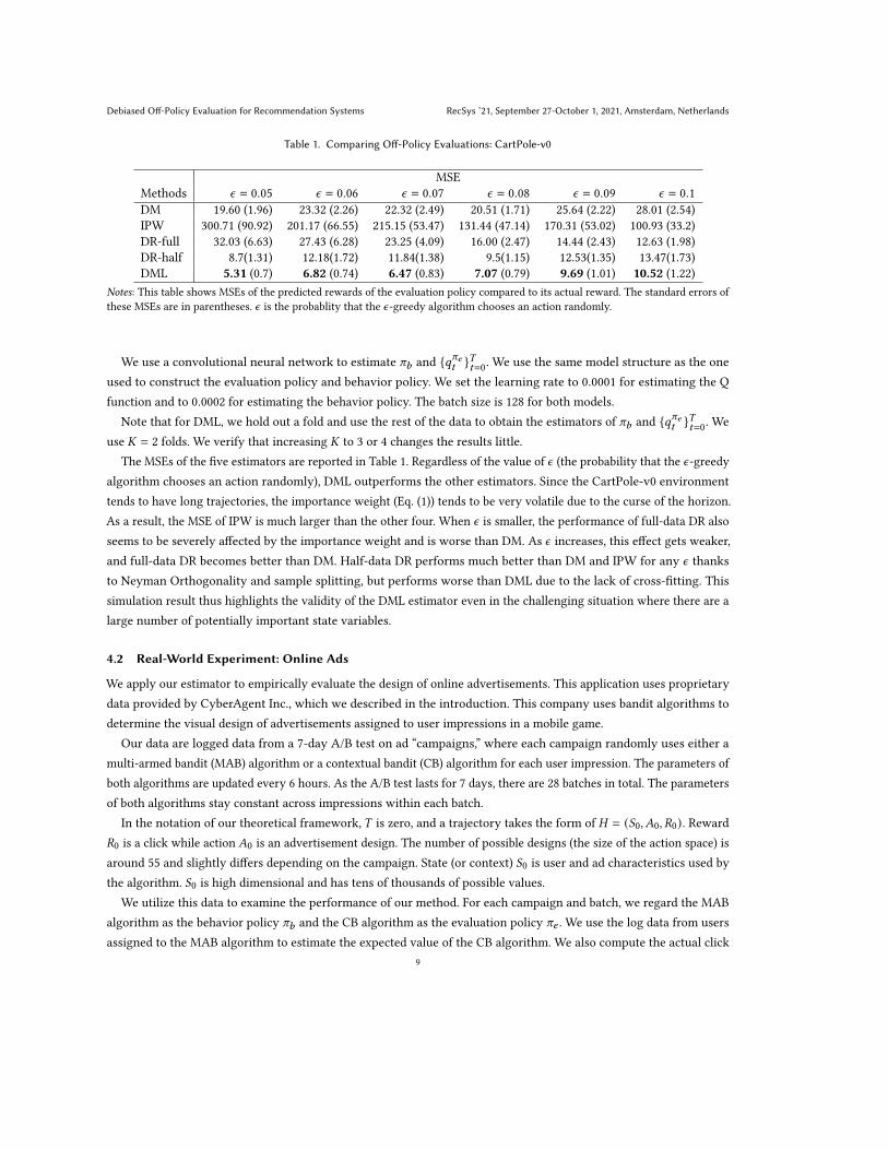
Table 1. Comparing Off-Policy Evaluations: CartPole-v0

MSE

Methods 𝜖 = 0.05 𝜖 = 0.06 𝜖 = 0.07 𝜖 = 0.08 𝜖 = 0.09 𝜖 = 0.1

DM 19.60 (1.96) 23.32 (2.26) 22.32 (2.49) 20.51 (1.71) 25.64 (2.22) 28.01 (2.54)

IPW 300.71 (90.92) 201.17 (66.55) 215.15 (53.47) 131.44 (47.14) 170.31 (53.02) 100.93 (33.2)

DR-full 32.03 (6.63) 27.43 (6.28) 23.25 (4.09) 16.00 (2.47) 14.44 (2.43) 12.63 (1.98)

DR-half 8.7(1.31) 12.18(1.72) 11.84(1.38) 9.5(1.15) 12.53(1.35) 13.47(1.73)

DML 5.31 (0.7) 6.82 (0.74) 6.47 (0.83) 7.07 (0.79) 9.69 (1.01) 10.52 (1.22)

Notes: This table shows MSEs of the predicted rewards of the evaluation policy compared to its actual reward. The standard errors of

these MSEs are in parentheses. 𝜖 is the probablity that the 𝜖-greedy algorithm chooses an action randomly.

We use a convolutional neural network to estimate 𝜋𝑏 and {𝑞𝜋𝑒𝑡 }𝑇𝑡=0

. We use the same model structure as the one

used to construct the evaluation policy and behavior policy. We set the learning rate to 0.0001 for estimating the Q

function and to 0.0002 for estimating the behavior policy. The batch size is 128 for both models.

Note that for DML, we hold out a fold and use the rest of the data to obtain the estimators of 𝜋𝑏 and {𝑞𝜋𝑒𝑡 }𝑇𝑡=0

. We

use 𝐾 = 2 folds. We verify that increasing 𝐾 to 3 or 4 changes the results little.

The MSEs of the five estimators are reported in Table 1. Regardless of the value of 𝜖 (the probability that the 𝜖-greedy

algorithm chooses an action randomly), DML outperforms the other estimators. Since the CartPole-v0 environment

tends to have long trajectories, the importance weight (Eq. (1)) tends to be very volatile due to the curse of the horizon.

As a result, the MSE of IPW is much larger than the other four. When 𝜖 is smaller, the performance of full-data DR also

seems to be severely affected by the importance weight and is worse than DM. As 𝜖 increases, this effect gets weaker,

and full-data DR becomes better than DM. Half-data DR performs much better than DM and IPW for any 𝜖 thanks

to Neyman Orthogonality and sample splitting, but performs worse than DML due to the lack of cross-fitting. This

simulation result thus highlights the validity of the DML estimator even in the challenging situation where there are a

large number of potentially important state variables.

4.2 Real-World Experiment: Online Ads

We apply our estimator to empirically evaluate the design of online advertisements. This application uses proprietary

data provided by CyberAgent Inc., which we described in the introduction. This company uses bandit algorithms to

determine the visual design of advertisements assigned to user impressions in a mobile game.

Our data are logged data from a 7-day A/B test on ad “campaigns,” where each campaign randomly uses either a

multi-armed bandit (MAB) algorithm or a contextual bandit (CB) algorithm for each user impression. The parameters of

both algorithms are updated every 6 hours. As the A/B test lasts for 7 days, there are 28 batches in total. The parameters

of both algorithms stay constant across impressions within each batch.

In the notation of our theoretical framework, 𝑇 is zero, and a trajectory takes the form of 𝐻 = (𝑆0, 𝐴0, 𝑅0). Reward𝑅0 is a click while action 𝐴0 is an advertisement design. The number of possible designs (the size of the action space) is

around 55 and slightly differs depending on the campaign. State (or context) 𝑆0 is user and ad characteristics used by

the algorithm. 𝑆0 is high dimensional and has tens of thousands of possible values.

We utilize this data to examine the performance of our method. For each campaign and batch, we regard the MAB

algorithm as the behavior policy 𝜋𝑏 and the CB algorithm as the evaluation policy 𝜋𝑒 . We use the log data from users

assigned to the MAB algorithm to estimate the expected value of the CB algorithm. We also compute the actual click

9


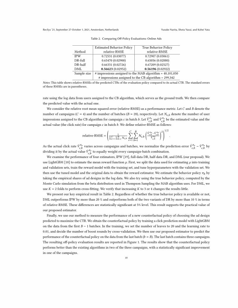
Table 2. Comparing Off-Policy Evaluations: Online Ads

Estimated Behavior Policy True Behavior Policy

Method relative-RMSE relative-RMSE

IPW 0.72531 (0.03077) 0.72907 (0.03061)

DR-full 0.65470 (0.02900) 0.65056 (0.02880)

DR-half 0.66331 (0.02726) 0.67209 (0.02527)

DML 0.56623 (0.02952) 0.56196 (0.02922)

Sample size # impressions assigned to the MAB algorithm = 40,101,050

# impressions assigned to the CB algorithm = 299,342

Notes: This table shows relative-RMSEs of the predicted CTRs of the evaluation policy compared to its actual CTR. The standard errors

of these RMSEs are in parentheses.

rate using the log data from users assigned to the CB algorithm, which serves as the ground truth. We then compare

the predicted value with the actual one.

We consider the relative root mean squared error (relative-RMSE) as a performance metric. Let 𝐶 and 𝐵 denote the

number of campaigns (𝐶 = 4) and the number of batches (𝐵 = 28), respectively. Let 𝑁𝑐,𝑏 denote the number of user

impressions assigned to the CB algorithm for campaign 𝑐 in batch 𝑏. Let 𝑉𝜋𝑒𝑐,𝑏

and 𝑉𝜋𝑒𝑐,𝑏

be the estimated value and the

actual value (the click rate) for campaign 𝑐 in batch 𝑏. We define relative-RMSE as follows:

relative-RMSE =

(1∑𝐶

𝑐=1

∑𝐵𝑏=1

𝑁𝑐,𝑏

𝐶∑︁𝑐=1

𝐵∑︁𝑏=1

𝑁𝑐,𝑏

(�̂�

𝜋𝑒𝑐,𝑏

−𝑉 𝜋𝑒𝑐,𝑏

𝑉𝜋𝑒𝑐,𝑏

)2

)1/2

.

As the actual click rate 𝑉𝜋𝑒𝑐,𝑏

varies across campaigns and batches, we normalize the prediction error 𝑉𝜋𝑒𝑐,𝑏

− 𝑉 𝜋𝑒𝑐,𝑏

by

dividing it by the actual value 𝑉𝜋𝑒𝑐,𝑏

to equally weight every campaign-batch combination.

We examine the performance of four estimators, IPW [19], full-data DR, half-data DR, and DML (our proposal). We

use LightGBM [10] to estimate the mean reward function `. First, we split the data used for estimating ` into training

and validation sets, train the reward model with the training set, and tune hyperparameters with the validation set. We

then use the tuned model and the original data to obtain the reward estimator. We estimate the behavior policy 𝜋𝑏 by

taking the empirical shares of ad designs in the log data. We also try using the true behavior policy, computed by the

Monte Carlo simulation from the beta distribution used in Thompson Sampling the MAB algorithm uses. For DML, we

use 𝐾 = 2 folds to perform cross-fitting. We verify that increasing 𝐾 to 3 or 4 changes the results little.

We present our key empirical result in Table 2. Regardless of whether the true behavior policy is available or not,

DML outperforms IPW by more than 20 % and outperforms both of the two variants of DR by more than 10 % in terms

of relative-RMSE. These differences are statistically significant at 5% level. This result supports the practical value of

our proposed estimator.

Finally, we use our method to measure the performance of a new counterfactual policy of choosing the ad design

predicted to maximize the CTR. We obtain the counterfactual policy by training a click prediction model with LightGBM

on the data from the first 𝐵 − 1 batches. In the training, we set the number of leaves to 20 and the learning rate to

0.01, and decide the number of boost rounds by cross-validation. We then use our proposed estimator to predict the

performance of the counterfactual policy on the data from the last batch (𝑏 = 𝐵). The last batch contains three campaigns.

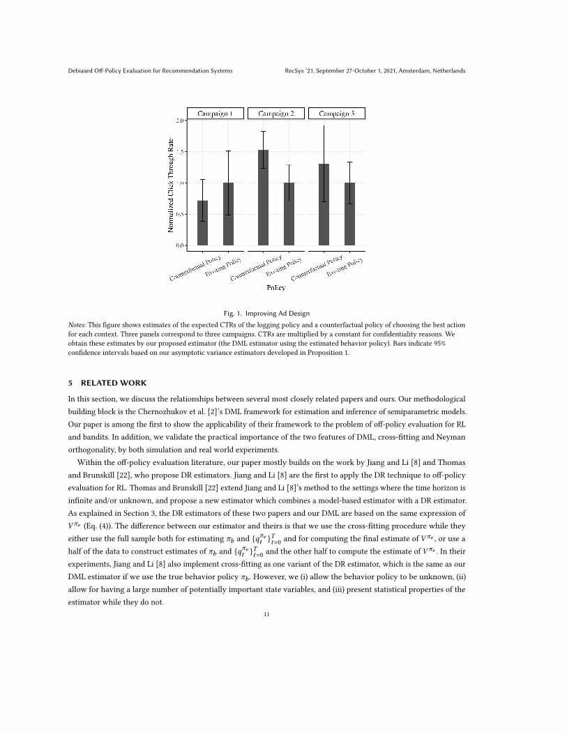
The resulting off-policy evaluation results are reported in Figure 1. The results show that the counterfactual policy

performs better than the existing algorithms in two of the three campaigns, with a statistically significant improvement

in one of the campaigns.

10


Fig. 1. Improving Ad Design

Notes: This figure shows estimates of the expected CTRs of the logging policy and a counterfactual policy of choosing the best action

for each context. Three panels correspond to three campaigns. CTRs are multiplied by a constant for confidentiality reasons. We

obtain these estimates by our proposed estimator (the DML estimator using the estimated behavior policy). Bars indicate 95%

confidence intervals based on our asymptotic variance estimators developed in Proposition 1.

5 RELATEDWORK

In this section, we discuss the relationships between several most closely related papers and ours. Our methodological

building block is the Chernozhukov et al. [2]’s DML framework for estimation and inference of semiparametric models.

Our paper is among the first to show the applicability of their framework to the problem of off-policy evaluation for RL

and bandits. In addition, we validate the practical importance of the two features of DML, cross-fitting and Neyman

orthogonality, by both simulation and real world experiments.

Within the off-policy evaluation literature, our paper mostly builds on the work by Jiang and Li [8] and Thomas

and Brunskill [22], who propose DR estimators. Jiang and Li [8] are the first to apply the DR technique to off-policy

evaluation for RL. Thomas and Brunskill [22] extend Jiang and Li [8]’s method to the settings where the time horizon is

infinite and/or unknown, and propose a new estimator which combines a model-based estimator with a DR estimator.

As explained in Section 3, the DR estimators of these two papers and our DML are based on the same expression of

𝑉 𝜋𝑒 (Eq. (4)). The difference between our estimator and theirs is that we use the cross-fitting procedure while they

either use the full sample both for estimating 𝜋𝑏 and {𝑞𝜋𝑒𝑡 }𝑇𝑡=0

and for computing the final estimate of 𝑉 𝜋𝑒 , or use a

half of the data to construct estimates of 𝜋𝑏 and {𝑞𝜋𝑒𝑡 }𝑇𝑡=0

and the other half to compute the estimate of 𝑉 𝜋𝑒 . In their

experiments, Jiang and Li [8] also implement cross-fitting as one variant of the DR estimator, which is the same as our

DML estimator if we use the true behavior policy 𝜋𝑏 . However, we (i) allow the behavior policy to be unknown, (ii)

allow for having a large number of potentially important state variables, and (iii) present statistical properties of the

estimator while they do not.

11


The most closely related paper to ours is Kallus and Uehara [9], who also apply DML to off-policy evaluation for

RL. Their work and our work are independent and simultaneous. More substantively, there are several key differences

between their paper and ours. Empirically, their paper does not have an application to a real dataset. In contrast, we

show the estimator’s practical performance in a real product setting. In addition, we provide a consistent estimator of

the asymptotic variance, and allow for having a large number of potentially important state variables while they do not.

Methodologically, their estimator differs from ours in that they estimate the marginal distribution ratioPr𝐻∼𝜋𝑒 (𝑆𝑡 ,𝐴𝑡 )Pr𝐻∼𝜋𝑏 (𝑆𝑡 ,𝐴𝑡 )

and plug it in place of 𝜌𝜋𝑒𝑡 (𝐻𝑠,𝑎𝑡 ;𝜋𝑏 ) of our estimator. There are tradeoffs between the two approaches. Their estimator

is better in that it has a smaller asymptotic variance. In the important case with a known behavior policy, however,

our estimator has the following advantages. (1) Our approach only needs to estimate {𝑞𝜋𝑒𝑡 }𝑇𝑡=0

, while their approach

needs to estimate the marginal distribution ratio as well as {𝑞𝜋𝑒𝑡 }𝑇𝑡=0

. (2) Our estimator is

√𝑁 -consistent and can be

asymptotic normal even when the nonparametric estimator of {𝑞𝜋𝑒𝑡 }𝑇𝑡=0

does not converge to the true one, or when the

parametric model of {𝑞𝜋𝑒𝑡 }𝑇𝑡=0

is misspecified. In contrast, their estimator may not be even consistent in such a case

unless the nonparametric estimator of the marginal distribution ratio is consistent, or the parametric model of the

marginal distribution ratio is correctly specified.

6 CONCLUSION

This paper proposes a new off-policy evaluation method, by marrying the DR estimator with Double/Debiased Machine

Learning. Our estimator has two features. First, unlike the IPW estimator, it is robust to the bias in the estimates of

the behavior policy and of the state-action value function (Neyman orthogonality). Second, we use a sample-splitting

procedure called cross-fitting. This removes the overfitting bias that would arise without sample splitting but still makes

full use of data, which makes our estimator better than DR estimators. Theoretically, we show that our estimator is√𝑁 -consistent and asymptotically normal with a consistent variance estimator, thus allowing for correct statistical

inference. Our experiments show that our estimator outperforms the standard DR, IPW and DM estimators in terms of

the mean squared error. This result not only demonstrates the capability of our estimator to reduce prediction errors,

but also suggests the more general possibility that the two features of DML (Neyman orthogonality and cross-fitting)

may improve many variants of the DR estimator such as MAGIC [21], SWITCH [24] and MRDR [5].

REFERENCES[1] Greg Brockman, Vicki Cheung, Ludwig Pettersson, Jonas Schneider, John Schulman, Jie Tang, and Wojciech Zaremba. 2016. OpenAI Gym. arXiv

preprint arXiv:1606.01540 (2016).[2] Victor Chernozhukov, Denis Chetverikov, Mert Demirer, Esther Duflo, Christian Hansen, Whitney Newey, and James Robins. 2018. Double/debiased

machine learning for treatment and structural parameters. The Econometrics Journal 21, 1 (2018), C1–C68.[3] Victor Chernozhukov, Juan Carlos Escanciano, Hidehiko Ichimura, Whitney K. Newey, and James M. Robins. 2018. Locally Robust Semiparametric

Estimation. Arxiv (2018).

[4] Miroslav Dudík, Dumitru Erhan, John Langford, and Lihong Li. 2014. Doubly Robust Policy Evaluation and Optimization. Statist. Sci. 29 (2014),485–511.

[5] Mehrdad Farajtabar, Yinlam Chow, and Mohammad Ghavamzadeh. 2018. More Robust Doubly Robust Off-policy Evaluation. In Proceedings of the35th International Conference on Machine Learning. 1447–1456.

[6] Alexandre Gilotte, Clément Calauzènes, Thomas Nedelec, Alexandre Abraham, and Simon Dollé. 2018. Offline A/B Testing for Recommender

Systems, In Proceedings of the Eleventh ACM International Conference on Web Search and Data Mining. WSDM, 198—-206.

[7] Alex Irpan, Kanishka Rao, Konstantinos Bousmalis, Chris Harris, Julian Ibarz, and Sergey Levine. 2019. Off-Policy Evaluation via Off-Policy

Classification. In Advances in Neural Information Processing Systems 32.[8] Nan Jiang and Lihong Li. 2016. Doubly Robust Off-policy Value Evaluation for Reinforcement Learning. In Proceedings of the 33rd International

Conference on Machine Learning. 652–661.

12


[9] Nathan Kallus and Masatoshi Uehara. 2020. Double Reinforcement Learning for Efficient Off-Policy Evaluation in Markov Decision Processes, In

Proceedings of the 37th International Conference on Machine Learning. ICML.[10] Guolin Ke, Qi Meng, Thomas Finley, Taifeng Wang, Wei Chen, Weidong Ma, Qiwei Ye, and Tie-Yan Liu. 2017. Lightgbm: A highly efficient gradient

boosting decision tree. In Advances in Neural Information Processing Systems 30. 3146–3154.[11] Lihong Li, Wei Chu, John Langford, and Robert E Schapire. 2010. A Contextual-bandit Approach to Personalized News Article Recommendation, In

Proceedings of the 19th International Conference on World Wide Web. WWW, 661–670.

[12] Lihong Li, Wei Chu, John Langford, and XuanhuiWang. 2011. Unbiased Offline Evaluation of Contextual-bandit-based News Article Recommendation

Algorithms, In Proceedings of the Fourth ACM International Conference on Web Search and Data Mining. WSDM, 297–306.

[13] Yao Liu, Omer Gottesman, Aniruddh Raghu, Matthieu Komorowski, Aldo A Faisal, Finale Doshi-Velez, and Emma Brunskill. 2018. Representation

balancing mdps for off-policy policy evaluation. In Advances in Neural Information Processing Systems 31. 2644–2653.[14] Yusuke Narita, Shota Yasui, and Kohei Yata. 2019. Efficient Counterfactual Learning from Bandit Feedback, In Proceedings of the 33rd AAAI

Conference on Artificial Intelligence. AAAI, 4634–4641.[15] Whitney K. Newey and James M. Robins. 2018. Cross-Fitting and Fast Remainder Rates for Semiparametric Estimation. Arxiv (2018).

[16] Adam Paszke, Sam Gross, Francisco Massa, Adam Lerer, James Bradbury, Gregory Chanan, Trevor Killeen, Zeming Lin, Natalia Gimelshein, Luca

Antiga, Alban Desmaison, Andreas Kopf, Edward Yang, Zachary DeVito, Martin Raison, Alykhan Tejani, Sasank Chilamkurthy, Benoit Steiner, Lu

Fang, Junjie Bai, and Soumith Chintala. 2019. PyTorch: An Imperative Style, High-Performance Deep Learning Library, In Advances in Neural

Information Processing Systems 32. NIPS, 8024–8035.[17] Doina Precup, Richard S. Sutton, and Satinder Singh. 2000. Eligibility Traces for Off-Policy Policy Evaluation, In Proceedings of the 17th International

Conference on Machine Learning. ICML, 759–766.[18] Andrea Rotnitzky and James M Robins. 1995. Semiparametric regression estimation in the presence of dependent censoring. Biometrika 82, 4 (1995),

805–820.

[19] Alex Strehl, John Langford, Lihong Li, and Sham M Kakade. 2010. Learning from Logged Implicit Exploration Data, In Advances in Neural

Information Processing Systems 23. NIPS, 2217–2225.[20] Adith Swaminathan, Akshay Krishnamurthy, Alekh Agarwal, Miro Dudik, John Langford, Damien Jose, and Imed Zitouni. 2017. Off-policy Evaluation

for Slate Recommendation, In Advances in Neural Information Processing Systems 30. NIPS, 3635–3645.[21] Philip Thomas and Emma Brunskill. 2016. Data-Efficient Off-Policy Policy Evaluation for Reinforcement Learning. In Proceedings of the 33rd

International Conference on Machine Learning. 2139–2148.[22] Philip Thomas and Emma Brunskill. 2016. Data-efficient Off-policy Policy Evaluation for Reinforcement Learning, In Proceedings of the 33rd

International Conference on Machine Learning. ICML, 2139–2148.[23] Masatoshi Uehara, Jiawei Huang, and Nan Jiang. 2020. Minimax Weight and Q-Function Learning for Off-Policy Evaluation, In Proceedings of the

37th International Conference on Machine Learning. ICML.[24] Yu-Xiang Wang, Alekh Agarwal, and Miroslav Dudik. 2017. Optimal and Adaptive Off-policy Evaluation in Contextual Bandits, In Proceedings of

the 34th International Conference on Machine Learning. ICML, 3589–3597.

13


APPENDICES

A EXAMPLES

The data generating process in our framework allows for many popular RL and bandit algorithms, as the following

examples illustrate.

Example 1 (Deep 𝑄 Learning). In each round 𝑡 , given state 𝑠𝑡 , a Q Learning algorithm picks the best action based

on the estimated Q-value of each actions, 𝑄 (𝑠, 𝑎), which estimates the expected cumulative reward from taking action 𝑎

(following the state and the policy). Choice probabilities can be determined with an 𝜖-greedy or soft-max rule, for instance.

In the case where the soft-max rule is employed, the probability of taking each action is as follows:

𝜋 (𝑎 |𝑠𝑡 ) =exp(𝑄 (𝑠𝑡 , 𝑎))∑

𝑎′∈𝐴 exp(𝑄 (𝑠𝑡 , 𝑎′)).

Deep Q Learning algorithms estimate Q-value functions through deep learning methods.

Example 2 (Actor Critic). An Actor Critic is a hybrid method of value-based approach such as Q learning and

policy-based method such as REINFORCE. This algorithm has two components called Actor and Critic. Critic estimates the

value function and Actor updates the policy using the value of Critic. In each round t, we pick the best action according

to the value of Actor with some probability. As in Deep 𝑄 Learning algorithms, we can use 𝜖-greedy and soft-max for

determining an action.

Contextual bandit algorithms are also important examples. When𝑇 = 0, a trajectory takes the form of𝐻 = (𝑆0, 𝐴0, 𝑅0).Regarding 𝑆0 as a context, it is possible to consider {𝐻𝑖 }𝑁𝑖=1

as batch data generated by a contextual bandit algorithm.

In additional examples below, the algorithms use past data to estimate the mean reward function ` and the reward

variance function 𝜎2

𝑅, where 𝜎2

𝑅(𝑠, 𝑎) =

∫(𝑟 − ` (𝑠, 𝑎))2𝑑𝑃𝑅 (𝑟 |𝑠, 𝑎). Let ˆ̀ and �̂�2

𝑅denote any given estimators of ` and

𝜎2

𝑅, respectively.

Example 3 (𝜖-greedy). When the context is 𝑠0, we choose the best action based on ˆ̀(𝑠0, 𝑎) with probability 1 − 𝜖 andchoose an action uniformly at random with probability 𝜖 :

𝜋 (𝑎 |𝑠0) =

1 − 𝜖 + 𝜖

|A | if 𝑎 = argmax

𝑎′∈Aˆ̀(𝑠0, 𝑎′)

𝜖|A | otherwise.

Example 4 (Thompson Sampling using Gaussian priors). When the context is 𝑠0, we sample the potential reward

𝑟0 (𝑎) from the normal distribution 𝑁 ( ˆ̀(𝑠0, 𝑎), �̂�2

𝑅(𝑠0, 𝑎)) for each action, and choose the action with the highest sampled

potential reward, argmax

𝑎′∈A𝑟0 (𝑎′). As a result, this algorithm chooses actions with the following probabilities:

𝜋 (𝑎 |𝑠0) = Pr(𝑎 = argmax

𝑎′∈A𝑟0 (𝑎′)),

where (𝑟0 (𝑎))𝑎∈A ∼ 𝑁 ( ˆ̀(𝑠0), Σ̂(𝑠0)), ˆ̀(𝑠0) = ( ˆ̀(𝑠0, 𝑎))𝑎∈A , and Σ̂(𝑠0) is the diagonal matrix whose diagonal entries are

(𝜎2

𝑅(𝑠0, 𝑎))𝑎∈A .

B ADDITIONAL FIGURE

We show some examples of visual ad designs in our real product application in Figure 2.

14


Fig. 2. Examples of Visual Ad Designs

C STANDARD ERROR CALCULATIONS IN THE ONLINE AD EXPERIMENT

We calculate the standard error (statistical uncertainty) of relative-RMSE by a bootstrap-like procedure. This procedure

is based on normal approximation of the distributions of 𝑉𝜋𝑒𝑐,𝑏

and 𝑉𝜋𝑒𝑐,𝑏

: for each (𝑐, 𝑏), 𝑉 𝜋𝑒𝑐,𝑏

∼ 𝑁 (𝑉 𝜋𝑒𝑐,𝑏,�̂�

2,𝑜𝑝𝑒

𝑐,𝑏

𝑁𝑜𝑝𝑒

𝑐,𝑏

) and


∼ 𝑁 (𝑉 𝜋𝑒𝑐,𝑏,�̂�

2,𝑜𝑛𝑙𝑖𝑛𝑒

𝑐,𝑏

𝑁𝑐,𝑏), where 𝑉 𝜋𝑒

𝑐,𝑏is the true value of policy 𝜋𝑒 , �̂�

2,𝑜𝑝𝑒

𝑐,𝑏is the estimator for the asymptotic variance of


given in Proposition 1, 𝑁𝑜𝑝𝑒

𝑐,𝑏is the number of impressions used to estimate 𝑉

𝜋𝑒𝑐,𝑏

, and �̂�2,𝑜𝑛𝑙𝑖𝑛𝑒

𝑐,𝑏= 𝑉

𝜋𝑒𝑐,𝑏

(1 −𝑉 𝜋𝑒𝑐,𝑏

) isthe sample variance of the click indicator among the impressions assigned to the CB algorithm.

The standard error is computed as follows. First, we compute �̂�2,𝑜𝑝𝑒

𝑐,𝑏and �̂�


𝑐,𝑏for each (𝑐, 𝑏). Second, we draw

𝑉𝜋𝑒 ,𝑠𝑖𝑚

𝑐,𝑏and𝑉

𝜋𝑒 ,𝑠𝑖𝑚

𝑐,𝑏independently from 𝑁 (𝑉 𝜋𝑒

𝑐,𝑏,�̂�

2,𝑜𝑝𝑒

𝑐,𝑏

𝑁𝑜𝑝𝑒

𝑐,𝑏

) and 𝑁 (𝑉 𝜋𝑒𝑐,𝑏,�̂�


𝑐,𝑏

𝑁𝑐,𝑏) for every (𝑐, 𝑏), and calculate the relative-

RMSE using the draws {(𝑉 𝜋𝑒 ,𝑠𝑖𝑚𝑐,𝑏

,𝑉𝜋𝑒 ,𝑠𝑖𝑚

𝑐,𝑏)}𝑐=1,...,𝐶,𝑏=1,...,𝐵 . We then repeat the second step 100,000 times, and compute

the standard deviation of the simulated relative-RMSEs.

D LEMMAS

Lemma 1. For 𝑡 = 0, ...,𝑇 , E𝐻∼𝜋𝑏 [𝜌𝜋𝑒𝑡 (𝐻𝑠,𝑎𝑡 )𝑅𝑡 ] = E𝐻∼𝜋𝑒 [𝑅𝑡 ].

Proof. Let 𝑃𝜋 (ℎ𝑠,𝑎𝑡 ) denote the probability of observing trajectory ℎ𝑠,𝑎𝑡 = (𝑠0, 𝑎0, ..., 𝑠𝑡 , 𝑎𝑡 ) when 𝐻 ∼ 𝜋 for some

policy 𝜋 . Under our data generating process,

𝑃𝜋 (ℎ𝑠,𝑎0

) = 𝑃𝑆0(𝑠0)𝜋 (𝑎0 |𝑠0),

and for 𝑡 ≥ 1,

𝑃𝜋 (ℎ𝑠,𝑎𝑡 ) =𝑃𝑆0(𝑠0)𝜋 (𝑎0 |𝑠0)𝑃𝑆 (𝑠1 |𝑠0, 𝑎0) × · · · × 𝑃𝑆 (𝑠𝑡 |𝑠𝑡−1, 𝑎𝑡−1)𝜋 (𝑎𝑡 |𝑠𝑡 ).

15


Hence, 𝑃𝜋𝑏 (ℎ𝑠,𝑎𝑡 )𝜌𝜋𝑒𝑡 (ℎ𝑠,𝑎𝑡 ) = 𝑃𝜋𝑒 (ℎ𝑠,𝑎𝑡 ) for any 𝑡 = 0, ...,𝑇 . We then have that

E𝐻∼𝜋𝑏 [𝜌𝜋𝑒𝑡 (𝐻𝑠,𝑎𝑡 )𝑅𝑡 ] = E𝐻∼𝜋𝑏 [𝜌

𝜋𝑒𝑡 (𝐻𝑠,𝑎𝑡 )E𝐻∼𝜋𝑏 [𝑅𝑡 |𝐻

𝑠,𝑎𝑡 ]]

= E𝐻∼𝜋𝑏 [𝜌𝜋𝑒𝑡 (𝐻𝑠,𝑎𝑡 )` (𝑆𝑡 , 𝐴𝑡 )]

=∑︁ℎ𝑠,𝑎𝑡

𝑃𝜋𝑏 (ℎ𝑠,𝑎𝑡 )𝜌𝜋𝑒𝑡 (ℎ𝑠,𝑎𝑡 )` (𝑠𝑡 , 𝑎𝑡 )


𝑃𝜋𝑒 (ℎ𝑠,𝑎𝑡 )` (𝑠𝑡 , 𝑎𝑡 )

= E𝐻∼𝜋𝑒 [` (𝑆𝑡 , 𝐴𝑡 )]

= E𝐻∼𝜋𝑒 [E𝐻∼𝜋𝑒 [𝑅𝑡 |𝐻𝑠,𝑎𝑡 ]]

= E𝐻∼𝜋𝑒 [𝑅𝑡 ],

where we use E𝐻∼𝜋𝑏 [𝑅𝑡 |𝐻𝑠,𝑎𝑡 ] = E𝐻∼𝜋𝑒 [𝑅𝑡 |𝐻

𝑠,𝑎𝑡 ] = ` (𝑆𝑡 , 𝐴𝑡 ), and we use 𝑃𝜋𝑏 (ℎ𝑠,𝑎𝑡 )𝜌𝜋𝑒𝑡 (ℎ𝑠,𝑎𝑡 ) = 𝑃𝜋𝑒 (ℎ𝑠,𝑎𝑡 ) for the

fourth equality. □

Lemma 2. E𝐻∼𝜋𝑏 [∑𝑇𝑡=0

𝛾𝑡 𝜌𝜋𝑒𝑡 (𝐻𝑠,𝑎𝑡 )𝑅𝑡 ] = 𝑉 𝜋𝑒 .

Proof. This immediately follows from Lemma 1 and the definition of 𝑉 𝜋𝑒 . □

Lemma 3. For 𝑡 = 0, ...,𝑇 and for any measurable function 𝑔𝑡 : (S × A)𝑡 → R, E𝐻∼𝜋𝑏 [𝜌𝜋𝑒𝑡 (𝐻𝑠,𝑎𝑡 )𝑔𝑡 (𝐻𝑠,𝑎𝑡 )] =

E𝐻∼𝜋𝑒 [𝑔𝑡 (𝐻𝑠,𝑎𝑡 )].

Proof. We have that

E𝐻∼𝜋𝑏 [𝜌𝜋𝑒𝑡 (𝐻𝑠,𝑎𝑡 )𝑔𝑡 (𝐻𝑠,𝑎𝑡 )] =

∑︁ℎ𝑠,𝑎𝑡

𝑃𝜋𝑏 (ℎ𝑠,𝑎𝑡 )𝜌𝜋𝑒𝑡 (ℎ𝑠,𝑎𝑡 )𝑔(ℎ𝑠,𝑎𝑡 )


𝑃𝜋𝑒 (ℎ𝑠,𝑎𝑡 )𝑔(ℎ𝑠,𝑎𝑡 )

= E𝐻∼𝜋𝑒 [𝑔𝑡 (𝐻𝑠,𝑎𝑡 )],

where we use 𝑃𝜋𝑏 (ℎ𝑠,𝑎𝑡 )𝜌𝜋𝑒𝑡 (ℎ𝑠,𝑎𝑡 ) = 𝑃𝜋𝑒 (ℎ𝑠,𝑎𝑡 ) for the second equality. □

Lemma 4. For 𝑡 = 1, ...,𝑇 and for anymeasurable function𝑔𝑡 : (S×A)𝑡−1×S → R, E𝐻∼𝜋𝑏 [𝜌𝜋𝑒𝑡−1


)𝑔𝑡 (𝐻𝑠,𝑎𝑡−1, 𝑆𝑡 )] =

E𝐻∼𝜋𝑒 [𝑔𝑡 (𝐻𝑠,𝑎𝑡−1

, 𝑆𝑡 )].

Proof. We have that

E𝐻∼𝜋𝑏 [𝜌𝜋𝑒𝑡−1


)𝑔𝑡 (𝐻𝑠,𝑎𝑡−1, 𝑆𝑡 )] =

∑︁(ℎ𝑠,𝑎

𝑡−1,𝑠𝑡 )

𝑃𝜋𝑏 (ℎ𝑠,𝑎𝑡−1

)𝑃𝑆 (𝑠𝑡 |𝑠𝑡−1, 𝑎𝑡−1) × 𝜌𝜋𝑒𝑡−1(ℎ𝑠,𝑎𝑡−1

)𝑔(ℎ𝑠,𝑎𝑡−1

, 𝑠𝑡 )

=∑︁

(ℎ𝑠,𝑎𝑡−1,𝑠𝑡 )

𝑃𝜋𝑒 (ℎ𝑠,𝑎𝑡−1

)𝑃𝑆 (𝑠𝑡 |𝑠𝑡−1, 𝑎𝑡−1)𝑔(ℎ𝑠,𝑎𝑡−1, 𝑠𝑡 )

= E𝐻∼𝜋𝑒 [𝑔𝑡 (𝐻𝑠,𝑎𝑡−1

, 𝑆𝑡 )],

where we use 𝑃𝜋𝑏 (ℎ𝑠,𝑎𝑡−1

)𝜌𝜋𝑒𝑡−1

(ℎ𝑠,𝑎𝑡−1

) = 𝑃𝜋𝑒 (ℎ𝑠,𝑎𝑡−1

) for the second equality. □

16


E PROOF OF PROPOSITION 1

We use Theorems 3.1 and 3.2 of Chernozhukov et al. [2] for the proof. We verify that E𝐻∼𝜋𝑏 [𝜓 (𝐻 ;[)] = 𝑉 𝜋𝑒 and that𝜓

satisfies the Neyman orthogonality condition. For the first part,

E𝐻∼𝜋𝑏 [𝜓 (𝐻 ;[)] =𝑇∑︁𝑡=0

𝛾𝑡E𝐻∼𝜋𝑏 [𝜌𝜋𝑒𝑡 (𝐻𝑠,𝑎𝑡 ) (𝑅𝑡 − 𝑞𝜋𝑒𝑡 (𝑆𝑡 , 𝐴𝑡 )) + 𝜌𝜋𝑒𝑡−1


)∑︁𝑎∈A

𝜋𝑒 (𝑎 |𝑆𝑡 )𝑞𝜋𝑒𝑡 (𝑆𝑡 , 𝑎)]

= 𝑉 𝜋𝑒 −𝑇∑︁𝑡=0

𝛾𝑡 {E𝐻∼𝜋𝑒 [𝑞𝜋𝑒𝑡 (𝑆𝑡 , 𝐴𝑡 )] − E𝐻∼𝜋𝑒 [

∑︁𝑎∈A

𝜋𝑒 (𝑎 |𝑆𝑡 )𝑞𝜋𝑒𝑡 (𝑆𝑡 , 𝑎)]}

= 𝑉 𝜋𝑒 −𝑇∑︁𝑡=0

𝛾𝑡 {E𝐻∼𝜋𝑒 [𝑞𝜋𝑒𝑡 (𝑆𝑡 , 𝐴𝑡 )]E𝐻∼𝜋𝑒 [𝑞

𝜋𝑒𝑡 (𝑆𝑡 , 𝐴𝑡 )]}

= 𝑉 𝜋𝑒 ,

where we use Lemmas 2, 3 and 4 for the second equality.

We now show that𝜓 satisfies the Neyman orthogonality condition. Let

𝐷𝜌𝜋𝑒𝑡 (𝐻𝑠,𝑎𝑡 ) [�̃�𝑏 ] B

𝜕𝜌𝜋𝑒𝑡 (𝐻𝑠,𝑎𝑡 ;𝜋𝑏 + 𝑟 (�̃�𝑏 − 𝜋𝑏 ))

𝜕𝑟

��𝑟=0

for any candidate �̃�𝑏 . Note that by Lemmas 3 and 4,

E𝐻∼𝜋𝑏 [−𝜌𝜋𝑒𝑡 (𝐻𝑠,𝑎𝑡 )𝑞𝜋𝑒𝑡 (𝑆𝑡 , 𝐴𝑡 ) + 𝜌𝜋𝑒𝑡−1


)∑︁𝑎∈A


= E𝐻∼𝜋𝑒 [−𝑞𝜋𝑒𝑡 (𝑆𝑡 , 𝐴𝑡 ) +

∑︁𝑎∈A


= E𝐻∼𝜋𝑒 [−𝑞𝜋𝑒𝑡 (𝑆𝑡 , 𝐴𝑡 )] + E𝐻∼𝜋𝑒 [𝑞

𝜋𝑒𝑡 (𝑆𝑡 , 𝐴𝑡 )]

= 0

for 𝑡 = 0, ...,𝑇 . We then have that for any candidate [̃ = (�̃�𝑏 , {𝑞𝜋𝑒𝑡 }𝑇𝑡=0

),

𝜕E𝐻∼𝜋𝑏 [𝜓 (𝐻 ;[ + 𝑟 ([̃ − [))]𝜕𝑟

��𝑟=0

=

𝑇∑︁𝑡=0

𝛾𝑡E𝐻∼𝜋𝑏 [𝐷𝜌𝜋𝑒𝑡 (𝐻𝑠,𝑎𝑡 ) [�̃�𝑏 ] (𝑅𝑡 − 𝑞𝜋𝑒𝑡 (𝑆𝑡 , 𝐴𝑡 )) − 𝜌𝜋𝑒𝑡 (𝐻𝑠,𝑎𝑡 )𝑞𝜋𝑒𝑡 (𝑆𝑡 , 𝐴𝑡 )

+ 𝐷𝜌𝜋𝑒𝑡−1


) [�̃�𝑏 ]∑︁𝑎∈A

𝜋𝑒 (𝑎 |𝑆𝑡 )𝑞𝜋𝑒𝑡 (𝑆𝑡 , 𝑎) + 𝜌𝜋𝑒𝑡−1(𝐻𝑠,𝑎𝑡−1

)∑︁𝑎∈A


=

𝑇∑︁𝑡=0

𝛾𝑡E𝐻∼𝜋𝑏 [𝐷𝜌𝜋𝑒𝑡 (𝐻𝑠,𝑎𝑡 ) [�̃�𝑏 ] (𝑅𝑡 − 𝑞𝜋𝑒𝑡 (𝑆𝑡 , 𝐴𝑡 )) + 𝐷𝜌𝜋𝑒𝑡−1


) [�̃�𝑏 ]∑︁𝑎∈A


= 𝛾𝑇E𝐻∼𝜋𝑏 [𝐷𝜌𝜋𝑒𝑇

(𝐻𝑠,𝑎𝑇

) [�̃�𝑏 ] (𝑅𝑇 − 𝑞𝜋𝑒𝑇

(𝑆𝑇 , 𝐴𝑇 ))]

+𝑇−1∑︁𝑡=0

𝛾𝑡E𝐻∼𝜋𝑏 [𝐷𝜌𝜋𝑒𝑡 (𝐻𝑠,𝑎𝑡 ) [�̃�𝑏 ] (𝑅𝑡 − 𝑞𝜋𝑒𝑡 (𝑆𝑡 , 𝐴𝑡 ) + 𝛾

∑︁𝑎∈A

𝜋𝑒 (𝑎 |𝑆𝑡+1)𝑞𝜋𝑒𝑡+1(𝑆𝑡+1, 𝑎))] .

17


SinceE𝐻∼𝜋𝑏 [𝑅𝑇 |𝐻𝑠,𝑎𝑇

] = ` (𝑆𝑇 , 𝐴𝑇 ) and𝑞𝜋𝑇𝑒 (𝑆𝑇 , 𝐴𝑇 ) = ` (𝑆𝑇 , 𝐴𝑇 ), the first term is zero by the law of iterated expectations.

The second term is also zero, since for 𝑡 = 0, ...,𝑇 − 1,

E𝐻∼𝜋𝑏 [𝐷𝜌𝜋𝑒𝑡 (𝐻𝑠,𝑎𝑡 ) [�̃�𝑏 ] (𝑅𝑡 + 𝛾

∑︁𝑎∈A

𝜋𝑒 (𝑎 |𝑆𝑡+1)𝑞𝜋𝑒𝑡+1(𝑆𝑡+1, 𝑎))]

= E𝐻∼𝜋𝑏 [𝐷𝜌𝜋𝑒𝑡 (𝐻𝑠,𝑎𝑡 ) [�̃�𝑏 ]E𝐻∼𝜋𝑏 [𝑅𝑡 + 𝛾

∑︁𝑎∈A

𝜋𝑒 (𝑎 |𝑆𝑡+1)𝑞𝜋𝑒𝑡+1(𝑆𝑡+1, 𝑎) |𝐻𝑠,𝑎𝑡 ]]

= E𝐻∼𝜋𝑏 [𝐷𝜌𝜋𝑒𝑡 (𝐻𝑠,𝑎𝑡 ) [�̃�𝑏 ] (` (𝑆𝑡 , 𝐴𝑡 ) + 𝛾

∑︁𝑠∈S

𝑃𝑆 (𝑠 |𝑆𝑡 , 𝐴𝑡 )∑︁𝑎∈A

𝜋𝑒 (𝑎 |𝑠)𝑞𝜋𝑒𝑡+1(𝑠, 𝑎))]

= E𝐻∼𝜋𝑏 [𝐷𝜌𝜋𝑒𝑡 (𝐻𝑠,𝑎𝑡 ) [�̃�𝑏 ]𝑞𝜋𝑒𝑡 (𝑆𝑡 , 𝐴𝑡 )],

where we use the recursive formulation of 𝑞𝜋𝑡 for the last equality.

The convergence results then follow from Theorems 3.1 and 3.2 of Chernozhukov et al. [2]. □

18

Documents

Debiased Off-Policy Evaluation for Recommendation Systems