Decentralizing Rent-seeking: Water and Power in

Pakistan’s Indus Basin∗

Hanan G. Jacoby† Ghazala Mansuri‡ Freeha Fatima§

August 16, 2017

Abstract

Does decentralizing public resource allocation reduce rent-seeking or merely change

its venue? We study a governance reform in Pakistan’s vast Indus basin irrigation sys-

tem. Using canal discharge measurements across all of Punjab, we find that water theft

increased on channels taken over by local farmer organizations, compared to channels

that remained bureaucratically managed, leading to substantial wealth redistribution.

This increase in water theft was also sharper along channels with larger landowners

situated upstream. These findings are consistent with a model in which decentraliza-

tion accentuates the political power of local elites by shifting the arena in which water

rights are contested.

∗Financial support for this project was provided by the Knowledge for Change Program. The viewsexpressed herein are those of the authors, and do not necessarily reflect the opinions of the World Bank, itsexecutive directors, or the countries they represent.†World Bank, 1818 H St NW, Washington DC 20433; e-mail: hjacoby@worldbank.org.‡World Bank; e-mail: gmansuri@worldbank.org.§World Bank; e-mail: ffatima@worldbank.org.

1 Introduction

Perceived corruption and lack of accountability associated with top-down public service deliv-

ery has led to calls for greater decentralization in developing countries. Indeed, participatory

or grass-roots governance, in which resource control resides with local elected bodies rather

than with centralized bureaucracies, has gained currency among international agencies and

donors (see, e.g., World Bank 2004), even though communal authority is by no means im-

mune from rent-seeking in its various forms. A key empirical question is, therefore, whether

the promise of local governance can be realized in practice and, if so, under what conditions.

Yet, empirical investigation is hampered by lack of large-scale ‘controlled’ experiments in

decentralization and by the paucity of objective data on rent-seeking behavior.1 This paper

takes advantage of a partial governance reform in the world’s largest canal irrigation system,

that of Pakistan’s Indus basin watershed. During the last decade, in an effort encouraged by

the World Bank, the management of several large sub-systems in the Punjab was transferred

from the provincial irrigation department to grass-roots farmer organizations (FOs) orga-

nized at the channel level. Here we assess how this shift from bureaucratic to local control

affected rent-seeking in the form of water “theft” along a channel.

Effective management of large irrigation systems has proven elusive in both historical and

contemporary experience (Meinzen-Dick, 2007).2 In the continuous gravity flow and rotation

systems most common in Asia, volumetric pricing and widespread water trading–i.e., market-

based allocation–faces daunting technical hurdles (Moore, 1989; Sampath, 1992).3 Instead,

1See Mansuri and Rao (2013) for a comprehensive and critical review of the evidence. A small literaturelooks at the impact of decentralization on corruption in cross-sections of countries (most recently, Fan et al.2009). The difficulties here include heterogeneity in the nature of decentralization and, of course, reversecausation (See Bardhan and Mookherjee 2006b).

2The celebrated writings of Elinor Ostrom take a slightly more optimistic view, arguing that self-governinginstitutions sometimes arise organically to solve collective action problems, at least in smaller-scale irrigationsystems (Ostrom and Garner 1993).

3Surface irrigation systems are distinct from other public utilities, such as piped water networks, in thatproperty rights are vastly cheaper to enforce in the latter case; canal water thus has an important commonproperty dimension.

1

irrigation bureaucracies have been established to operate and monitor centralized systems

for the allocation of water as it makes its way down from the rivers and main canals to

the network of distributaries, minor and sub-minor canals, and, finally, to the watercourse

outlets, where it is distributed to individual farms. In such quota-based systems, users have

a strong temptation to bribe local officials to “look the other way” as they use various means

to illicitly enhance their water entitlement. Invariably, such water theft benefits farmers at

the head of the channel, where water is first to arrive, at the expense of farmers at the tail

(see Bromely et al. 1980, Wade 1982, and Chambers 1988). As even a cursory internet

search reveals, canal water theft garners enormous media attention in Pakistan, where it is

often portrayed as pitting large landlords at the head against multitudes of poor tail-enders.

While decentralization strips authority from unelected irrigation department bureaucrats,

farmer organizations may also be subject to capture by these upstream elites and, hence, may

sanction as much (if not more) water theft than the irrigation department functionaries they

replace. In this sense, irrigation reform and, more broadly, decentralization could merely

change the venue for rent-seeking without ameliorating its underlying causes.4 To think

about the implications of decentralizing irrigation management, we set out a simple model

of water allocation, corruption, and rent-seeking along a canal system. Given the locational

asymmetry, corruption and theft are concentrated at the head of a channel. However, theft

induces rent-seeking by coalitions of gainers (farmers at the head) and losers (farmers at the

tail); these coalitions have varying degrees of political influence. Under irrigation depart-

ment control, lobbying effort is directed “over the head” of the local official involved in the

corruption whereas, under decentralized control, it is directed toward the FO. The model

4Rijsberman (2008) elaborates on the view that so-called water users associations are not a panacea. Pun-jab’s irrigation reform exemplifies what Meinzen-Dick (2007) terms “externally initiated programs...[with]top-down imposition of a rigid structure of user groups and uniform rules that would allow state agenciesto recognize and interact with [them].” Such irrigation management transfers, according to her review ofthe evidence, have had mixed success. Vermillion (1997), considering much the same body of country case-studies, concludes that “the literature on irrigation management transfer does not yet allow analysts to drawstrong conclusions about...impacts, either positive or negative.” p29.

2

has several empirical implications for the impact of decentralization and how this impact

interacts with asymmetry in political influence.

The centerpiece of our analysis of Pakistan’s irrigation reform is an administrative database

maintained by the Punjab Irrigation Department and consisting of readings taken from wa-

ter discharge gauges installed at the head and tail of each channel of the entire system.

These data arguably provide an objective measure of water theft along a channel. More-

over, water discharge data are available over the years 2006-2014, a period encompassing

significant devolution of irrigation management to FOs. Importantly, we are also able to

match villages along each irrigation channel back to unit record landownership data from

recent Agricultural Censuses. This allows us to construct measures of differences in political

power, proxied by landholdings, between head and tail villages and thus establish whether

irrigation reform has had heterogeneous impacts along this dimension.

In a companion paper (Jacoby and Mansuri 2017), we study the allocation of canal water

in the presence of rent-seeking farmers and of corruptible irrigation officials with career

concerns. Using data from several hundred distributaries in Punjab that were not subject

to irrigation reform, we find that, under bureaucratic control, the extent of water theft is

substantially affected by the distribution of political power along a channel: where political

influence is relatively concentrated at the head of a channel, water allocations are more

favorable toward the head as reflected in land value differentials between head and tail. In

this paper, by contrast, we focus on how inequality interacts with decentralization. Although

the literature recognizes that local governance is more likely to serve the interests of elites

where political power is more asymmetric (see Mansuri and Rao, 2013), empirical support

for this proposition has up to now been lacking.

We adopt two strategies for constructing a control group against which we compare the

changes in canal water allocations following decentralization. Since FOs were phased-in

starting in 2005, our first strategy is to look solely at variation in outcomes across distribu-

3

taries with early and late FO formation while controlling for channel-level fixed effects. In

this ‘pipeline’ approach, we only focus on the administrative zones where FO formation has

been sanctioned; those FOs that became operational later serve as controls for those that be-

came operational early. Our second, and ultimately preferable, strategy uses geographically

matched controls drawn from adjacent administrative zones in which provincial authorities

have not (yet) called for FOs to be established. That is, control channels are chosen on

the basis of being within a geographical buffer zone of given distance around a particular

FO channel. In this case, and in contrast to the pipeline strategy, we compare changes in

discharges over the same time period between FO and non-FO channels.5

To summarize our empirical results, we find strong evidence of an economically important

decrease in the relative allocation of water to the tail of a channel once an FO becomes

operational. Moreover, this decline is greater along FO channels where large landowners are

more heavily concentrated at the head vis a vis the tail. This latter finding implies that,

where power asymmetry is in the same direction as the inherent locational (head versus tail)

asymmetry, decentralization leads to greater inequity in allocations. By contrast, where the

power asymmetry and the inherent locational asymmetry work in opposition, the negative

impact of decentralization is muted.

This study contributes to a growing micro-empirical literature on the impact of decen-

tralization. Alatas et al. (2013) and Beath et al. (2017) look for direct evidence of elite

capture based on field experiments (in Indonesia and Afghanistan, respectively) in which the

authority or accountability of extant local governments is randomly varied (see also Basurto

et al., 2015, for a nonexperimental study along similar lines). None of these studies, however,

compares local-level to top-down control, the pre-reform scenario considered in this paper.

Moreover, as noted by Mookherjhee (2015), empirical work to date focuses almost exclusively

on intracommunity allocations, although “effects of decentralization on intercommunity al-

5Similarly, Holmes (1998) exploits legislative discontinuities at the borders of US states.

4

locations are no less important,” precisely because much rent-seeking activity is undertaken

by groups of actors in pursuit of their collective interests. Bardhan and Mookherjee (2006c),

using longitudinal data from West Bengal, find that district and/or state allocated develop-

ment grants to villages are strongly negatively related to the percentage of low-caste poor

households in the village. However, neither this study nor any other econometric analysis of

which we are aware addresses whether devolution of resource control can exacerbate conflict

and inequality between communities.

More broadly, this paper is related to, and the results consistent with, Acemoglu and

Robinson (2008) who study the interaction between de jure and de facto political power: “A

change in political institutions that modifies the distribution of de jure power,” they argue,

“need not lead to a change in equilibrium economic institutions if it is associated with an

offsetting change in the distribution of de facto political power.” Our question, in particular,

is whether an institutional change (decentralization) reduces economic inequality or is instead

thwarted by increased investments in political capture. We also follow Baland and Robinson

(2008) and Anderson et al. (2015), among others, in associating land ownership in developing

countries with political power or influence, although our mechanism (rent-seeking) is distinct

from theirs (clientilism).

The next section of the paper presents the institutional backdrop and data for our anal-

ysis. Section 3 develops the model of corruption and rent-seeking along a canal system.

Section 4 lays out the empirical methodologies and presents the main impacts of irrigation

management reform in Punjab. Section 5 turns to the empirical analysis of power asymmetry

along a channel and how it interact with decentralization. Section 6 concludes the paper.

5

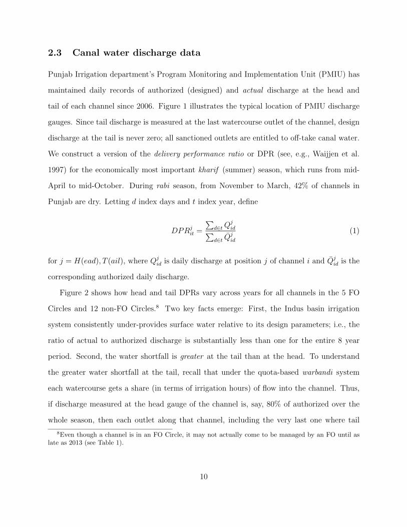
Head outlets and watercourses

Tail outlets and watercourses

Dis

trib

uta

ry

Minor canal

Outlet discharge

Distance from head0

= PMIU discharge gauge

Branch canal Authorized

ActualDe-silted

Figure 1: Channel schematic with discharge gauges

2 Context and Data

2.1 Indus Basin irrigation system

The Indus Basin irrigation system, which accounts for 80% of Pakistan’s agricultural produc-

tion, lies mostly in its most populous province, Punjab, wherein it encompasses 23 thousand

miles of canals and irrigates about 21 million acres. From the Indus, Jhelum, Chenab, Ravi,

and Sutlej rivers, issue a dense network of main canals, branch canals, distributaries, minors,

and sub-minors, ultimately feeding 58 thousand individual watercourses in Punjab alone (See

Figure 1 for a schematic of the canal hierarchy.).

Each watercourse outlet or mogha supplies irrigation to typically several dozen farmers

according to a rotational system known as warabandi. Tracing its origins to British colonial

rule and to the early development of irrigation in the Indus basin, the institution of warabandi

(literally “fixed turns”) embodies a modified principle of equity: to each irrigator in propor-

6

tion to his cultivated area. As discussed below, adherence to warabandi leads to an efficient

allocation of canal water. At each level of the canal hierarchy in this continuous gravity-flow

irrigation system, “authorized discharge” is allocated in proportion to cultivable command

area (CCA). At the main canal level, irrigation department staff operate a series of gates

regulating flow into the off-taking distributaries according to a rotational schedule. However,

since moghas are ungated, discharge into tertiary units, the watercourses, is determined by

the width of the outlet; the greater the watercourse CCA, the greater the authorized outlet

width (for a given canal discharge), and thus the greater the water in-take each week. Over

the course of a week, proceeding from the head to the tail of the watercourse, each farmer

takes his pre-assigned turn at using the entire flow to irrigate his field, with the length of

turn proportional to the size of the field.

Although design discharge at any point along a channel accounts for seepage and con-

veyance losses and is therefore a declining function of distance to the head (see Figure 1

inset), tail outlets should, in theory at least, receive their full water entitlement. In practice,

however, discharge at the distributary head is often too low (Bandaragoda and Rehman

1995), or the canal is too silted up, for water to reach the tail outlets. Over-silting also re-

sults in higher water levels at the channel head and, consequently, greater discharge at head

outlets (Van Waijjen et al. 1997). Lack of canal maintenance, therefore, tends to favor head

outlets, which may give rise to lobbying of the irrigation department by farmers at the tail

outlets to increase maintenance and by those at the head outlets to suppress it. Although

such manipulation is difficult to confirm,6 pervasive “direct” forms of water theft – i.e., tam-

pering with outlets to increase width, siphoning off canal water with pipes, breaching of the

canal banks, all undertaken with the connivance of corrupt irrigation officials – have been

documented in the Indus basin (Rinaudo 2002; Rinaudo et al. 2000).

6Yet, one apparently widespread practice having the same effect is placing large boulders or other ob-structions in the bed of a minor canal to increase flow at the head.

7

2.2 Irrigation management reform

Administratively, Punjab’s irrigation System is divided into 17 Circles (see Appendix Figure

B.1). As part of the reform, Area Water Boards (AWBs) were established at the Circle

level with the responsibility of promoting the formation of FOs covering every water channel

within the Circle, with the FOs themselves tasked with the operations and management of

distributaries and their off-taking channels. In particular, an FO is responsible for monitoring

the rotational system to ensure equitable allocation along the distributary, for mediating and

reporting water-related disputes among its irrigators, and for collecting water taxes to fund

canal operations and maintenance. Five AWBs in what we will refer to as “FO Circles” were

initially sanctioned to form FOs. Subsequent roll-out to the remaining 12 Circles has been

indefinitely delayed by concerns about FO performance.

The formation of an FO involves the following steps: First, an outlet level chairman is

elected by all landowners in each watercourse. Second, a secret ballot election is held at

the level of the distributary (including off-taking channels), through which a nine-member

management committee (president, vice-president, secretary, treasurer, and five executive

members) is selected from among the outlet level chairmen. The management committee

exercises all powers of the FO. Once elected, an FO does not start operations until its

members are trained and it is registered with the AWB.7 Once operationalized, the FO

membership remains in office for a tenure of three years, after which new elections are

due. In practice, this electoral system has not functioned smoothly. Several incumbent FOs

initiated legal action to remain in power and their first tenures have been extended beyond

the 3-year term under court stays.

Starting from the universe of 2902 irrigation channels in the Punjab, dropping cases

that either had zero discharge at the head throughout the 2006-14 period or in which the

7In theory, FO members were to acquire formal training related to the daily operations and managementof the system and be provided with ongoing institutional support. However, despite detailed rules andregulations to this effect, training and capacity building efforts stalled after the pilot phase in LCC East.

8

overseeing FO included a larger branch canal (3 FOs in all), leaves 2860 channels. Of these,

1007 are in FO Circles, covered by 394 FOs, and 1853 are in non-FO Circles. The excess

of channels over FOs in the former case reflects the fact that most distributaries have off-

taking minors (and sub-minors) for which we also have discharge data. A distributary-level

FO manages all of these minor canals as well. Appendix Table B.1 presents descriptive

statistics for all channels by FO status of the Circle. Across design features (number and

location of outlets, position along parent channel), FO and non-FO circles look quite similar.

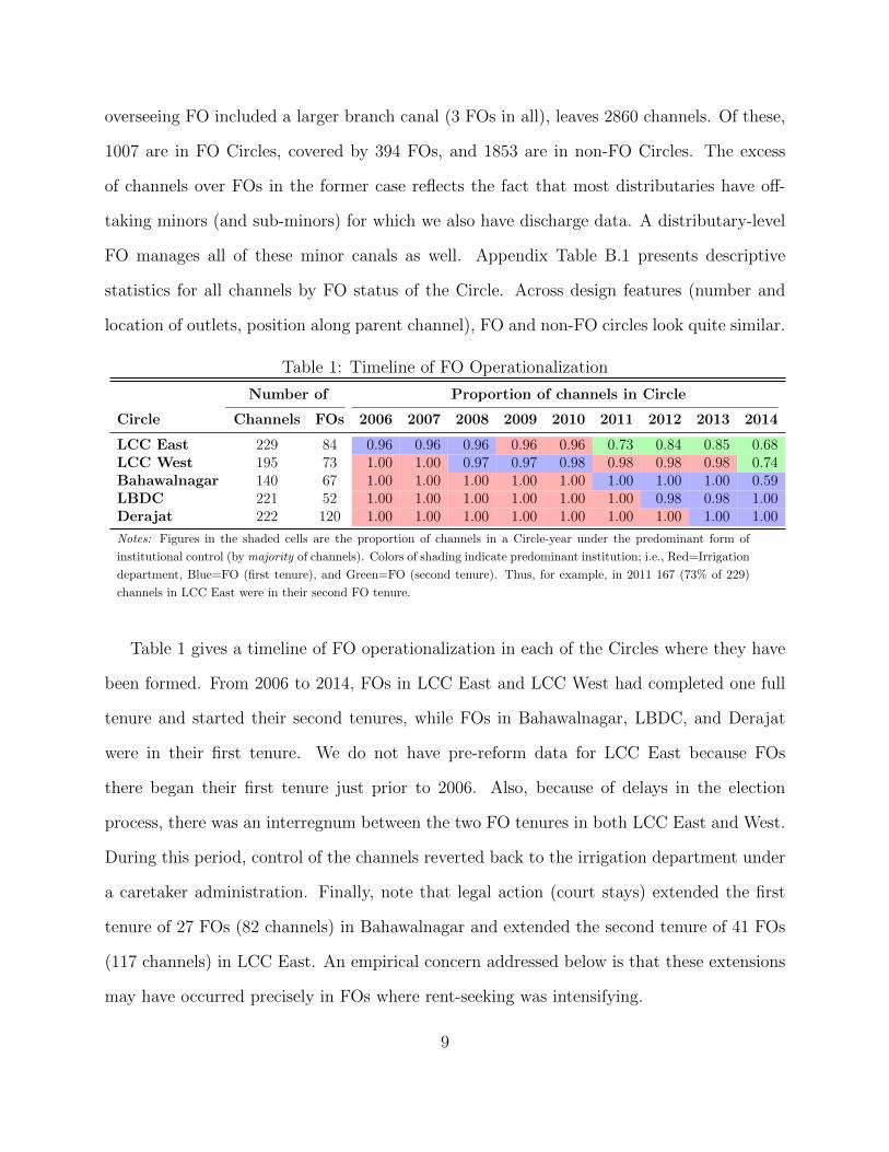
Table 1: Timeline of FO Operationalization

Number of Proportion of channels in Circle

Circle Channels FOs 2006 2007 2008 2009 2010 2011 2012 2013 2014

LCC East 229 84 0.96 0.96 0.96 0.96 0.96 0.73 0.84 0.85 0.68LCC West 195 73 1.00 1.00 0.97 0.97 0.98 0.98 0.98 0.98 0.74Bahawalnagar 140 67 1.00 1.00 1.00 1.00 1.00 1.00 1.00 1.00 0.59LBDC 221 52 1.00 1.00 1.00 1.00 1.00 1.00 0.98 0.98 1.00Derajat 222 120 1.00 1.00 1.00 1.00 1.00 1.00 1.00 1.00 1.00

Notes: Figures in the shaded cells are the proportion of channels in a Circle-year under the predominant form of

institutional control (by majority of channels). Colors of shading indicate predominant institution; i.e., Red=Irrigation

department, Blue=FO (first tenure), and Green=FO (second tenure). Thus, for example, in 2011 167 (73% of 229)

channels in LCC East were in their second FO tenure.

Table 1 gives a timeline of FO operationalization in each of the Circles where they have

been formed. From 2006 to 2014, FOs in LCC East and LCC West had completed one full

tenure and started their second tenures, while FOs in Bahawalnagar, LBDC, and Derajat

were in their first tenure. We do not have pre-reform data for LCC East because FOs

there began their first tenure just prior to 2006. Also, because of delays in the election

process, there was an interregnum between the two FO tenures in both LCC East and West.

During this period, control of the channels reverted back to the irrigation department under

a caretaker administration. Finally, note that legal action (court stays) extended the first

tenure of 27 FOs (82 channels) in Bahawalnagar and extended the second tenure of 41 FOs

(117 channels) in LCC East. An empirical concern addressed below is that these extensions

may have occurred precisely in FOs where rent-seeking was intensifying.

9

2.3 Canal water discharge data

Punjab Irrigation department’s Program Monitoring and Implementation Unit (PMIU) has

maintained daily records of authorized (designed) and actual discharge at the head and

tail of each channel since 2006. Figure 1 illustrates the typical location of PMIU discharge

gauges. Since tail discharge is measured at the last watercourse outlet of the channel, design

discharge at the tail is never zero; all sanctioned outlets are entitled to off-take canal water.

We construct a version of the delivery performance ratio or DPR (see, e.g., Waijjen et al.

1997) for the economically most important kharif (summer) season, which runs from mid-

April to mid-October. During rabi season, from November to March, 42% of channels in

Punjab are dry. Letting d index days and t index year, define

DPRjit =

∑d∈tQ

jid∑

d∈t Qjid

(1)

for j = H(ead), T (ail), where Qjid is daily discharge at position j of channel i and Qj

id is the

corresponding authorized daily discharge.

Figure 2 shows how head and tail DPRs vary across years for all channels in the 5 FO

Circles and 12 non-FO Circles.8 Two key facts emerge: First, the Indus basin irrigation

system consistently under-provides surface water relative to its design parameters; i.e., the

ratio of actual to authorized discharge is substantially less than one for the entire 8 year

period. Second, the water shortfall is greater at the tail than at the head. To understand

the greater water shortfall at the tail, recall that under the quota-based warbandi system

each watercourse gets a share (in terms of irrigation hours) of flow into the channel. Thus,

if discharge measured at the head gauge of the channel is, say, 80% of authorized over the

whole season, then each outlet along that channel, including the very last one where tail

8Even though a channel is in an FO Circle, it may not actually come to be managed by an FO until aslate as 2013 (see Table 1).

10

0.2

.4.6

.81

2006 2008 2010 2012 2014 2006 2008 2010 2012 2014

FO Circles Non-FO Circles

Head TailActual/authorized discharge

Figure 2: Head and Tail DPRs by year for FO and non-FO channels

discharge is measured, would automatically receive 80% of its water entitlement or design

flow. If, however, upstream outlets are enlarged or the canal is breached or silt is not removed

in a timely manner, then off-take per hour at the head is increased and relatively less water

makes its way to the tail of the channel over the course of the season; for any given value of

DPRH , there is a lower value of DPRT .

As noted earlier, however, water theft in its various forms is not the only reason for

differential shortages at channel tails. Fluctuation in the flow of water into the channel during

the week also disrupts the warabandi schedule. Absent a continuous discharge throughout

the week at the head, the channel would not remain full and tail outlets would not receive

water. To examine this issue, we again use the daily data to construct the coefficient of

variation (CV) of weekly discharge at the head of each channel. Note that we take the

intertemporal variance of weekly discharge within each kharif season so that CV varies by

both channel and year. Figure 3 shows a strong positive relationship between tail shortage,

11

-.05

0.0

5.1

Hea

d D

PR

- Ta

il D

PR

5th pctile 95th pctileCV of weekly kharif head discharge

95% CI lpoly smoothNote: CV trimmed below 1st and above 99th percentile

Figure 3: Head-tail differences in DPR as a function of CV

defined as

TSit = DPRHit −DPRT

it (2)

and the variability of seasonal discharge across most of the range of CVs. It is, therefore,

important to control for CV in the empirical analysis.

Returning to Figure 2, the average tail shortage across all channels and years is twice as

large in FO Circles (0.096) as in non-FO Circles (0.048). Since this gap is not attributable to

differences in average CVs between FO and non-FO Circles, which are negligible, it appears

that water theft is more prevalent in FO Circles. However, inferring anything about the

causal impact of FOs is premature. Indeed, the pattern could reflect selection; i.e., reforms

may have been initiated in areas where water theft was most pervasive to begin with.

12

3 Conceptual Framework

3.1 Centralized bureaucracy versus decentralization

Modelling public service delivery both under centralized bureaucracy and under local gov-

ernance using a common theoretical apparatus poses a distinct challenge. In perhaps the

only attempt to do so,9 Bardhan and Mookherjee (2006a) consider a bureaucratic hierarchy

engaged in rent extraction under asymmetric information and compare it against a local

elected government captured by elites. Decentralization “shifts control rights away from

bribe extractors to those who respond to the interests of local users, owing to electoral pres-

sures. However, they respond with a bias in favour of local elites” (p. 110). Bribe-taking is,

consequently, replaced by biased fiscal transfers.

Bardhan and Mookherjee’s conceptualization of bureaucracy ignores the disciplining

power of career concerns. In a companion paper (Jacoby and Mansuri 2017), we develop a

model of canal water allocation in the presence of corruptible irrigation department officials

motivated by a dismissal or transfer threat. Here, we extend the model to cover the case

of FO-managed channels. Under either form of management, corruption generates winners

(farmers at the head of the channel) and losers (farmers at the downstream outlets) who

receive less water than they are entitled to. Rent-seeking arises as these winners and losers

lobby the powers-that-be to intercede on their behalf. To highlight the role of institutional

structure, the only difference between centralized and decentralized systems lies in the in-

centive for corruption, which, in equilibrium, affects the incentive for rent-seeking.

9Hoffmann et al. (2017) examine political allocations under centralized and decentralized structures whenhome constituencies are favored. However, there is no bureaucratic hierarchy in the model.

13

3.2 Model preliminaries

Assume a continuum of outlets along a channel indexed by n ∈ [0, N ], with n = 0 representing

the first outlet at the head of the channel and n = N the last outlet at the tail of the channel.

Suppose that each outlet has the same command area, normalized to one, and hence the

same de jure endowment of water w0. The de facto inflow of water to each outlet is given

by the function w(n), which for the channel as a whole is constrained by

∫ N

0

w(n)dn = Nw0. (3)

Agricultural output depends on water per acre cultivated, but with diminishing marginal

product.10 The demand schedule for water D(w) is, therefore, downward sloping (D′ < 0

for ∀w). Suppose further that D(w0) > 0 and that surplus from off-take w is

s(w) =

∫ w

0

D(w)dw. (4)

So, the de jure allocation has a positive marginal value and confers a collective surplus or

total value of s0 = s(w0) to farmers on the outlet.

The efficient allocation of canal water along a channel maximizes

∫ N

0

s(w(n))dn (5)

subject to (3), which requires that D(w(n)) be equal across outlets. The de jure allocation,

with w(n) = w0 ∀ n, is thus efficient and deviations from equal per acre allocations, such as

those discussed below, create deadweight losses.11

10Output, of course, also depends on purchased inputs such as seed and fertilizer, but to the extentthat these are optimally chosen and that their prices do not vary along a channel, the presence of suchcomplementary (to water) investments will not affect our analysis.

11Chakravorty and Roumasset (1993) point out that equal per-acre allocation along a canal is not neces-sarily efficient once conveyance losses–i.e., water seepage into the channel itself–are taken into account. They

14

3.3 Theft and corruption

Assume that canal water at each outlet is appropriated until its marginal value is zero subject

to availability. Since water arrives first at the head of the channel, outlets at the head have

first-mover advantage; some outlets at the tail must, therefore, get no water. Define outlet

off-take w such that D(w) = 0 and the ‘critical’ outlet n by nw = Nw0 (using equation 3).

Thus, all outlets n ∈ [0, n] off-take w − w0 in excess of their legal entitlement and receive

surplus s = s(w), whereas all outlets n ∈ (n, N ] receive no water and get zero surplus.

Now, consider the role of an authority, such as the irrigation department or an FO.

While the authority could, at some cost, set w < w by restricting outlet tampering and

other such violations, we assume that the amount of water theft w − w0 is, for them, a fait

accompli. Alternatively, we may suppose that the authority (through its agent) engages in

Nash bargaining with each outlet over w, which also yields w = w.12 In any case, the official

of the authority accepts a bribe from each offending outlet to overlook the infraction.13 If

the official cannot pre-commit to a bribe amount b for the entire channel, then b would also

be determined at each outlet in a Nash bargain (see fn. 12) and thus set to a fixed share

of excess surplus s − s0. However, inability to commit to a channel-level corruption plan

implies that political institutions and rent-seeking can have no influence on the official’s

actions. Therefore, for the sake of argument, we assume the contrary.

show that, in this case, optimal inflow at each outlet should decline with distance to the head. Chakravortyand Roumasset’s simulations, however, indicate that these conveyance loss effects only become quantitativelyrelevant for outlets at a considerable distance from the head. With a median length of 7 kilometers, thechannels that we consider are, in general, too short for conveyance losses to be consequential. Moreover,these simulations overstate the effect of canal seepage in our context by not accounting for the resultingaquifer recharge, which is recovered and used productively by farmers through groundwater pumping.

12In particular, w would be chosen to max [s(w)− s0 − b]η b1−η, where b is the bribe and η is an exogenousbargaining weight. The necessary condition for an optimum implies that s′(w) = D(w) = 0.

13Wade’s (1982, p. 297) observations from south India are apposite in this regard: “The distinctionbetween a bribe, offered by farmers to get the [irrigation official] to do something he might not otherwisedo, and extortion money, demanded by the officer in return for not inflicting a penalty, is often difficult todraw in practice.”

15

3.4 Rent-seeking

Water theft creates groups of winners (head outlets) and losers (tail outlets), each of which

lobbies the “powers-that-be” for its desired outcome. The head coalition CH = n|n ∈ [0, n]

and the tail coalition CT = n|n ∈ (n, N ] each try to sway the authority to, respectively,

continue the corruption or to end the corruption and restore the de jure water allocation. As

in Tullock (1980), we assume that the probability P of CH winning this rent-seeking contest

depends on the effort level, ej, of both coalitions j = H,T as follows:14

P =ιHeH

ιHeH + ιT eT, (6)

where the ιj represent the marginal influence of coalition j. When ιH 6= ιT , there is a power

asymmetry along the channel; this is the sense in which intercommunity inequality matters

for outcomes.15

Assuming a unitary marginal cost of effort,16 expected net surplus for CH is

πH = Pn(s− b) + (1− P )ns0 − eH (7)

= ns0 + P∆H − eH ,

where ∆H = n(s− s0 − b), and for CT is

πT = (1− P )(N − n)s0 − eT (8)

= (N − n)s0 − P∆T − eT14The linearity of each player’s effort in the probability function is a standard simplification in the literature

on games of rent-seeking (see Nitzan 1994).15Insofar as some of the rent-seeking effort translates into utility for the authority, there is an incentive

for whoever is in charge to hold a lobbying contest with non-trivial win probabilites for each side.16This assumption, applied to lobbying effort by both head and tail coalitions, is innocuous. High (low)

marginal influence ιj is equivalent to low (high) marginal cost of effort.

16

where ∆T = (N − n)s0.

We assume that each coalition chooses its rent-seeking effort taking that of the other

coalition as given. Assuming an interior solution,17 eT = ΩeH , where Ω = ∆T/∆H is the

ratio of win-loss differentials. Thus, in the Nash equilibrium, P = P , where

P (b) =ιH∆H(b)

ιH∆H(b) + ιT∆T

. (9)

The equilibrium probability of maintaining corruption depends on each coalition’s net gains

from winning the lobbying contest weighted by their marginal influence. We may write

equation (9) more compactly as

P (b) =θ

θ + Ω(b). (10)

where θ = ιH/ιT is a parameter representing the relative influence of the head coalition

vis-a-vis the tail coalition.

3.5 Optimal control of water theft

Bureaucracy: Bureaucracy is characterized by hierarchy; the official on the ground, di-

rectly engaged in corruption, is an agent of a higher level office. We assume that the local

official is, in effect, paid an efficiency wage and thus has career concerns (see Jacoby and

Mansuri 2017 and the citations therein). As long as he stays in his current position he

receives bribe income nb; otherwise, he receives his outside option, which we normalize to

zero. Whether the local official is retained depends on the pressure exerted on the irrigation

department by the contending interests along the channel. If CH wins the lobbying contest,

as described formally in the previous subsection, the corrupt official will be retained, whereas

if CT wins, the official will be ‘detected’ and reassigned (or fired). For simplicity, we suppose

that once the corrupt official leaves, he is replaced, at least temporarily, by a non-corrupt

17For sufficiently low ιT , eT = eH = 0 is optimal and political influence plays no role in water allocation.

17

regime under direct irrigation department oversight.18

The local official chooses his bribe b for the channel to maximize expected income

VB(b) = P (b)nb. (11)

Thus, the official faces a trade-off between greater bribe income, on the one hand, and a

higher equilibrium probability of retaining his position, on the other. In particular, the

higher the bribe, the less net surplus is available to head outlets and, hence, the less effort

their coalition exerts to retain the official.

Farmer Organizations: While FO officials are assumed to be just as corrupt as the

local irrigation department officials, their objective function differs in a key respect. Under

bureaucratic control, lobbying is directed upward, to the office with the authority to fire

or transfer the corrupt official. In a decentralized structure, farmers lobby the FO and at

least part of this lobbying directly benefits FO officials. Decentralization thus breaks the

separation between corruption and rent-seeking that prevails in the bureaucratic hierarchy.

Suppose that the FO receives utility u(b) = U(eT (b) + eH(b)) from the total rent-seeking

effort expended. We may think of u as the perks of power or the value of political support

to remain in power or to be reelected, or all three. The FO chooses b to maximize

VF (b) = P (b)nb+ u(b). (12)

VF combines the local irrigation official’s objective VB with that of the higher-level depart-

ment office, which we previously could (and did) ignore. Importantly, since u′ < 0 (higher

bribes, by curtailing total rent-seeking effort, make the FO worse off), the FO official has

lower marginal corruption incentives than the irrigation official and, hence, charges a lower

18Again, it would be in the interest of the irrigation department to provide for such a (credible) regimeprecisely to extract rents through the lobbying contest (see fn. 15).

18

bribe (see lemma 1, Appendix A).

3.6 Implications of decentralization

Our outcome variable, tail shortage, is the expected difference in water available at the first

and last outlet of a channel. In terms of the model, TSr = P (br)(w− 0) +[1− P (br)

](w0−

w0) = P (br)w, where r = B,F denote bureaucracy and FO, respectively. The model yields

three results (see Appendix A for proofs):

Proposition 1. TSF > TSB

This result says that water theft increases after decentralization, or ∆TS = TSF −TSB > 0.

Intuitively, the bribe amount falls under FO authority because, as noted, the marginal

incentives for bribery are reduced. Water theft, however, is decreasing in the bribe amount,

because higher bribes reduce head outlets’ surplus and, hence, their support for the status

quo (so P must fall).

Next, we have that decentralization increases water theft by more on channels along

which head outlets are relatively powerful; i.e., along those with high θ:

Proposition 2.∂∆TS

∂θ> 0.

Essentially, theft responds more to political influence when bribes are low (i.e., under FOs).19

Lastly, we have a symmetry result following directly from the definition θ = ιH/ιT :

Proposition 3.∂∆T

∂ log ιH= − ∂∆T

∂ log ιT.

A one percent increase in head influence has an equivalent effect on the change in tail shortage

as a one percent decrease in tail influence.

In the remainder of the paper, we take these implications of decentralization to the data.

19Jacoby and Mansuri (2017) prove that ∂TS(bB)/∂θ > 0 so that water theft is increasing in θ under bothirrigation department and FO authority.

19

4 Main Impact of Irrigation Reform

4.1 Pipeline strategy

Our baseline regression model for tail shortage, exploiting the pipeline variation, is

Yit = α1τ1it + α2τ

2it + β logCVit + µi + δt + γct+ εit (13)

where the τ jit are indicators for whether channel i is in the midst of its first (j = 1) or

second (j = 2) FO tenure during kharif season of year t. As noted, we control for the

seasonal CV of weekly head discharge as well as for channel fixed effects, µi, which sweep out

permanent channel characteristics, including those correlated with the likelihood of receiving

an FO earlier rather than later. We also include year dummies δt and Circle-specific time-

trends, as represented by the penultimate term in equation (13). Difference-in-differences

(or fixed effects) estimation of treatment effects is typically predicated on the parallel trends

assumption, which is to say that, absent intervention, average outcomes would have evolved

similarly for both treatment and control groups. Here, with the exception of LCC East,

which has no pre-reform observations (see Table 1), we are able to estimate separate time

trends, γc, for each FO Circle. Thus, we directly control for differential pre-intervention time

trends across the unit of policy choice (recall that Area Water Boards for the formation of

FOs were established at the Circle level).

4.2 Pipeline results

Results for the pipeline approach using all channel-years (Table 2, column 1) indicate that the

first FO tenure significantly increased tail shortage. The average treatment effect estimate

of 0.063 translates into 68% of the average pre-reform tail shortage across all FO channels

and years (0.092). Thus, the irrigation reform worsened discharge at the tail relative to

20

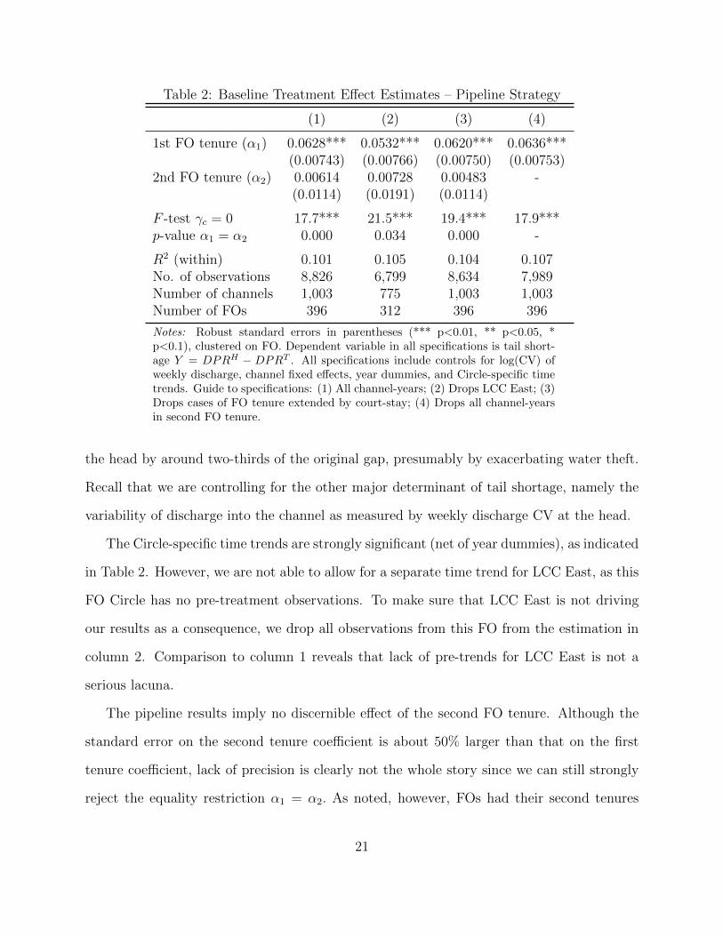
Table 2: Baseline Treatment Effect Estimates – Pipeline Strategy

(1) (2) (3) (4)

1st FO tenure (α1) 0.0628*** 0.0532*** 0.0620*** 0.0636***(0.00743) (0.00766) (0.00750) (0.00753)

2nd FO tenure (α2) 0.00614 0.00728 0.00483 -(0.0114) (0.0191) (0.0114)

F -test γc = 0 17.7*** 21.5*** 19.4*** 17.9***p-value α1 = α2 0.000 0.034 0.000 -

R2 (within) 0.101 0.105 0.104 0.107No. of observations 8,826 6,799 8,634 7,989Number of channels 1,003 775 1,003 1,003Number of FOs 396 312 396 396

Notes: Robust standard errors in parentheses (*** p<0.01, ** p<0.05, *p<0.1), clustered on FO. Dependent variable in all specifications is tail short-age Y = DPRH − DPRT . All specifications include controls for log(CV) ofweekly discharge, channel fixed effects, year dummies, and Circle-specific timetrends. Guide to specifications: (1) All channel-years; (2) Drops LCC East; (3)Drops cases of FO tenure extended by court-stay; (4) Drops all channel-yearsin second FO tenure.

the head by around two-thirds of the original gap, presumably by exacerbating water theft.

Recall that we are controlling for the other major determinant of tail shortage, namely the

variability of discharge into the channel as measured by weekly discharge CV at the head.

The Circle-specific time trends are strongly significant (net of year dummies), as indicated

in Table 2. However, we are not able to allow for a separate time trend for LCC East, as this

FO Circle has no pre-treatment observations. To make sure that LCC East is not driving

our results as a consequence, we drop all observations from this FO from the estimation in

column 2. Comparison to column 1 reveals that lack of pre-trends for LCC East is not a

serious lacuna.

The pipeline results imply no discernible effect of the second FO tenure. Although the

standard error on the second tenure coefficient is about 50% larger than that on the first

tenure coefficient, lack of precision is clearly not the whole story since we can still strongly

reject the equality restriction α1 = α2. As noted, however, FOs had their second tenures

21

in only two of the five FO circles (see in Table 1); in fact, 84% of these observations are

from LCC East, which, recall, was intended to be a showcase for the irrigation reform.

Additionally, as also noted, a large proportion of second tenures in LCC East were extended

by court stays. To check robustness against the concern that FO tenures were endogenously

extended by legal action, we drop all such channel-year observations (whether in the first or

second FO tenures) in column 3. The results are virtually unchanged. Finally, in the last

column of Table 1, we present the estimate for the first FO tenure treatment effect when

all second tenure observations are dropped. Again, there is essentially no difference between

this specification and that in column 1.

4.3 Spatial matching strategy

Before setting out the regression model for use with spatially matched controls, we discuss our

GIS buffer strategy. A buffer is a locus of GIS coordinates equidistant from each coordinate

of an FO channel. Spatial matching consists in finding the set of channels from non-FO

Circles that lie entirely within a buffer of given radius. Figure 4 illustrates a 40 kilometer

buffer for a channel in Bahawalnagar Circle along with one particular control channel, of

which there are typically many.20

The choice of radius for the GIS buffer presents a tradeoff. The smaller the radius, the

more similar treatment and control channels are likely to be along unobserved dimensions

(given spatial correlation in these unobservables). However, a smaller radius also implies a

smaller likelihood of finding any channels lying both within the buffer and within an adjacent

non-FO Circle. A radius of 40 km, in particular, leads to a sample consisting of 302 FOs

covering 747 channels, with 915 non-FO channels as controls (but each of these typically

appearing in many buffers). Thus, the choice of 40 km radius implies a loss of 94 of our

20There are no GIS shape files for Circle borders, so we cannot match on the basis of distance to theseadministrative boundaries.

22

Figure 4: Example of 40 km buffer for spatial matching

original 396 FOs in the sense that we do not have spatially matched controls for them. By

contrast, moving to a 60 km buffer radius matches 348 FOs covering 883 channels (with

1233 non-FO control channels). But shrinking the buffer radius down to 20 km nets only

130 FOs covering a mere 351 channels; since we believe that this is too few to constitute a

useful sample, we do not pursue the 20 km buffer strategy.

Indexing buffers by subscript b, our regression model becomes

Yibt = α1τ1it + α2τ

2it + β logCVit + µi + γct+ φbt + εibt (14)

where φbt is a buffer-year fixed effect.21 To understand the source of identifying variation

in equation (14), let us simplify the model so that we have just two time periods, before

and after reform. First-differencing over time for each channel in this case is equivalent to

21Due to the high dimensionality of both the channel and buffer-year fixed effects, we must estimateequation (14) using an iterative technique (Guimaraes and Portugal, 2010).

23

channel fixed effects and yields

∆Yibt = α1∆τ1it + α2∆τ

2it + β∆ logCVit + γc + φb + ∆εib, (15)

where φb is a buffer fixed effect. Thus, the average treatment effect of an FO tenure is iden-

tified off of within buffer variation in channel-level discharge differences (pre/post) between

FO and non-FO channels that lie in adjacent FO and non-FO Circles, respectively. In con-

trast to the pipeline approach, the spatial matching estimator uses none of the variation in

the timing of reform across FO Circles ; this is for the simple reason that, by construction, a

given buffer only contains channels from one FO Circle. Note that, because they are based

on different samples, regression models (14) and (13) are not nested and, hence, cannot be

readily tested against one another.

Finally, even though the general time-pattern of tail shortage is absorbed in the buffer-

year fixed effects included in equation (14), Circle-specific trends γc are still identified because

FOs from the same Circle appear in many different buffers. Indeed, it is important to control

for Circle-specific trends since it is conceivable that tail shortages in FO Circles and in

adjacent non-FO Circles were not on parallel trajectories prior to decentralization.22

4.4 Spatial matching results

22Our analysis of pre-trends in the three late-reforming FOs (Bahawalnagar, LBDC, and Derajat; seeTable 1) is summarized in Appendix Figure B.2. While parallel trends between these FOs and all non-FOchannels from 2006-2010 can be formally rejected, this is no longer the case when 2006 data are dropped.Below, therefore, we check our estimates for robustness to the removal of 2006 observations.

24

Table 3: Baseline Treatment Effect Estimates – Spatial Matching

40 km buffer 60 km buffer

(1) (2) (3) (4) (5) (6) (7) (8)

1st FO tenure (α1) 0.0480*** 0.0478*** - 0.0520*** 0.0441*** 0.0439*** - 0.0462***(0.00881) (0.00882) (0.00866) (0.00864) (0.00864) (0.00849)

2nd FO tenure (α2) 0.0505*** 0.0504*** - - 0.0369*** 0.0367*** - -(0.0169) (0.0169) (0.0141) (0.0140)

FO tenure (α1 = α2) - - 0.0485*** - - - 0.0425*** -(0.00806) (0.00743)

F -test γc = 0 6.8*** 6.8*** 7.1*** 6.2*** 7.2*** 7.2*** 7.8*** 7.0***p-value α1 = α2 0.894 0.888 - - 0.658 0.663 - -

R2 (within) 0.601 0.601 0.601 0.601 0.570 0.570 0.570 0.571Observations 223,109 222,970 223,109 222,508 674,296 674,121 674,296 673,517Number of clusters 751 751 751 751 916 916 916 916Number of FOs 302 302 302 302 348 348 348 348

Notes: Robust standard errors in parentheses (*** p<0.01, ** p<0.05, * p<0.1), clustered on FO/distributary (distributary for non-FOchannels). Dependent variable in all specifications is tail shortage Y = DPRH −DPRT . All specifications include controls for log(CV)of weekly discharge, channel fixed effects, buffer-year fixed effects, and Circle-specific time trends. Guide to specifications: (1,5) Allchannel-years; (2,6) Drops cases of FO tenure extended by court-stay; (3,7) Constrains α1 = α2; (4,8) Drops all channel-years in secondFO tenure.

25

The spatial matching strategy yields estimates of the first FO tenure treatment effect

that are similar in magnitude to those from the pipeline strategy, regardless of whether we

adopt a 40 km (Table 3, column 1) or a 60 km (column 5) buffer radius. Relative to the

pre-reform scenario in FO Circles, the first tenure effects imply a 52% (40 km buffer) and

48% (60 km buffer) incresae in tail shortage. In contrast to the pipeline case, however, the

second FO tenure effects here are statistically significant and of similar magnitude to the first

tenure effects, so that we cannot reject the equality restriction α1 = α2. Moreover, none of

these results depends on the inclusion of the potentially suspect observations involving court

stays (cols. 2 and 6). The rest of Table 3 reports specifications that restrict first and second

FO tenure effects to be equal (columns 3 and 7) and specifications that drop channel-years

in second FO tenures altogether (columns 4 and 8). All of these various treatment effects

are within a range of 10% of each other, i.e., well within a single standard error.23

4.5 Discussion

Two distinct panel data strategies have yielded broadly consistent findings: Irrigation reform

in Punjab increased tail shortage initially (i.e., in the first FO tenure) by at least 50% relative

to the pre-reform baseline. Since, as we have argued, the efficient allocation of canal water

involves zero tail shortage, decentralization had a social cost. In other words, the takeover

by FOs could not both accentuate head-tail inequality in canal water and (through side-

payments) lead to a Pareto improvement of welfare. While we cannot compute the social

cost directly, outlet-level data on land values from Punjab (see Jacoby and Mansuri 2017)

allow us to infer that the wealth redistribution was substantial; in particular, the reform

23Equality of Circle-specific time-trends can also be rejected in all specifications. Note, as well, thatdropping observations from 2006, thereby rendering parallel the pre-trends in FO and non-FO circles (seefn. 22), does not appreciably affect our results (the estimate of α1 in spectication (5) falls to 0.041 (0.009)and that of α2 falls to 0.030 (0.014)).

26

increased the value of head-end land by about 9% relative to the value of tail-end land.24

Evidence on the second FO tenure, which is far less frequent in the data than the first

tenure, is not as clear-cut. Results depend importantly upon the estimation strategy, which

is to say upon the comparison group. When the comparison group consists of channels

in other FO circles in the same years that were not in their second FO tenures (pipeline

strategy), we find no effect of second FO tenure. But, when the comparison group is non-FO

channels lying in the same 40 or 60 km buffer, we find a positive effect on tail shortage; in

particular, we cannot reject the null that first and second tenure effects are identical. Since

there is no theoretical reason to suggest that these effects should differ, we will rely on the

spatial matching strategy in the analysis to follow.

5 Role of Political Influence

Under what conditions will decentralization produce more equitable allocations? Our the-

oretical model formalizes the political process at the canal level as a rent-seeking contest

between rival coalitions of irrigators. Asymmetry of political influence (θ) thus affects the

outcome of irrigation reform. The empirical challenge is to measure the relative influence of

outlets at the head versus those at the tail. In Pakistan, the natural proxy for political power

is land ownership.25 Despite active tenancy markets, land sales markets are thin in Pakistan,

with the vast bulk of ownership transferred through inheritance. As a consequence, the local

distribution of land ownership can be seen as both stable and as largely independent of the

24The data come from a survey of around 4000 outlets along 470 non-FO channels in Punjab. Withinthe same channel, land at the head is valued at a 11.1% premium over land at the tail. Moreover, theDPR on these same channels (averaged over 2012-14) is higher by 0.055 at the head than at the tail.Assuming, plausibly, that the entire head-tail land value differential is attributable to variation in canalwater availability, a treatment effect of 0.044 is tantamount to a 11.1 × 0.044/0.055 = 8.9% increase inrelative land values.

25In Jacoby and Mansuri (2017), we use both landownership and political/bureaucratic/hereditary office-holding as proxies for political power. However, because the latter variables are only available for 470 non-FOchannels in Punjab, they are excluded from the present analysis.

27

distribution of farmer productivity or soil fertility (factors which are, at any rate, purged

from our regression specifications using channel fixed effects).

5.1 Land ownership data and mouza matching

We use data from four Agricultural Censuses (1980, 1990, 2000, and 2010) to characterize

the distribution of landownership along Punjab’s irrigation channels. Since Pakistan carries

out a “sample census,” about 13% of villages (mouzas) are covered in any given round (and

9% of households), yielding roughly 3500 villages per round with considerable overlap across

rounds. Thus, between 1980-2010, nearly 7700 unique villages appear in the Agricultural

Census. Given the relative stability of the land ownership distribution over time, we treat the

most recent observations on all of these villages equally for the purposes of constructing our

aggregates.26 Irrigated villages from the census are matched to their corresponding canal

outlets using village-outlet lists supplied by the Punjab irrigation department. Following

irrigation department designation, head villages are defined as those that match to outlets

on the upper 40% by length of a given channel; tail villages as those that match to outlets

on the lower 20%.

We compute land ownership statistics by position on the channel. For instance, mean

landholdings at the head is a household (population weighted) average based on unit record

data from all irrigated census villages that match to head outlets; likewise, for mean land-

holdings at the tail.27 To the extent that large landowners are the dominant source of

political influence, we compute the 90th percentiles of land ownership, in addition to the

means, at each channel position. Since the Agricultural Census does not provide household

landownership broken down by irrigated and rain-fed areas, even though it is the former that

is most germane to the lobbying effort along a channel, we deflate household landownership

26To the extent that land ownership data from the 1980s and 1990s are dated, they introduce measurementerror biasing against finding (differential) treatment effects.

27We drop any channel-position with fewer than 20 household level observations.

28

by the ratio of cultivated area under irrigation to total cultivated area in the mouza.

Note that the Agricultural Census samples all types of households within each mouza,

whether cultivating or not and whether they own land or not. Arguably, the population

of cultivators and/or landowners is most relevant for the political-economy of irrigation.

Since non-cultivating households without land should have little, if any, influence with the

FO, or with the irrigation department for that matter, this population might reasonably be

excluded in calculating channel position-level land statistics. On the other hand, includ-

ing these non-farm households could have an important scaling function. For example, a

community of a hundred households each owning a hundred acres is likely to have more

influence than a community consisting of just a single hundred-acre farm surrounded by 99

non-farm households; yet, mean landholdings across farm households is identical in these

two communities, whereas mean landholdings across all households is indeed higher in the

presumptively more powerful one. Of course, if the second community, instead, consisted

of a hundred hundred-acre farms and a hundred non-farm households, the mean across all

households would imply that the second is less powerful than the first when it is, in fact,

equally powerful. In this case, using the means across farm households would (correctly)

imply communities with identical lobbying influence. In short, for our purposes, there is no

unambiguously valid choice of population over which to compute land ownership statistics.

Prudence, therefore, dictates using both approaches.

Because the four rounds of sample census data are not everywhere dense in villages, we

are not able to match both head and tail mouzas for every channel. Our analysis of power

asymmetry is, thus, based on fewer FOs than were present in the baseline samples. For the

60 km spatial matching sample, the number of FOs covered falls from 349 to 247, when land

statistics are taken over only farm households, and to 252, when land statistics are taken

over all census households.28 There is also a modest (positive) correlation between land

28Of the 247 FOs represented in the former case, 15% are in Bahawalnagar Circle, 29% are in Derajat,

29

ownership statistics at head and tail of the same channel (see Appendix Figure B.3), which

is why these variables must be included together in the regressions.

5.2 Heterogeneity results

With these considerations, we now specify a mapping from the land distribution at position j

of the channel to relative political influence of the form ιj(L) ∝ exp(L). Thus, if we choose to

represent the distribution of landholdings by the mean, L, we would have log θi = LiH− LiT ,

where Lij, j = H,T, is mean landownership on position j of channel i. Taking the spatial

matching case, the augmented specification (dropping second FO tenure effects) is

Yibt = α1τ1ibt + δHτ

1ibtLiH + δT τ

1ibtLiT + β logCVit + µi + γct+ φbt + εibt. (16)

Under the symmetry restriction δH = −δT (see Proposition 3), this regression is equivalent to

interacting the treatment dummy with log θi. Symmetry, however, implies that head outlets

obtain just as much additional influence over allocations at the margin from (say) one acre

higher mean landownership at the head as from one acre lower mean landownership at

the tail. Although this restriction emerges from our simple model of rent-seeking and the

assumption that ιH(·) = ιT (·), we would rather test δH = −δT than impose it a priori.

17% are in LBDC, 21% are in LCC East, and 17% are in LCC West. The corresponding breakdown acrossall 396 FOs in Punjab is 17%, 30%, 13%, 21%, and 18%. In line with this similarity in composition, maintreatment effects are very close to those in Table 3 when estimated on the smaller samples of channels withland data (results available upon request).

30

Table 4: Influence Asymmetry and FO Performance

Census Farm Households All Census Households

Mean 90th percentile Mean 90th percentile

τ 1 (α1) 0.0502** 0.0547*** 0.0547*** 0.0551*** 0.0647*** 0.0578*** 0.0662*** 0.0574***(0.0212) (0.0109) (0.0197) (0.0109) (0.0183) (0.0107) (0.0204) (0.0108)

τ 1 × LH (δH) 0.00558** - 0.00181 - 0.00834** - 0.00343** -(0.00230) - (0.00117) - (0.00357) - (0.00157) -

τ 1 × LT (δT ) -0.00466 - -0.00178 -0.0107** - -0.00460** -(0.00319) - (0.00111) - (0.00473) - (0.00208) -

τ 1 × (LH − LT ) - 0.00518*** - 0.00179** - 0.00933*** - 0.00388***- (0.00194) - (0.000842) - (0.00308) - (0.00130)

p-value δH = −δT 0.810 - 0.984 - 0.657 - 0.636 -

R2 0.571 0.571 0.571 0.571 0.570 0.570 0.570 0.570No. of Obs. 586,417 586,417 586,417 586,417 602,425 602,425 602,425 602,425No. of clusters 892 892 892 892 909 909 909 909No. of FOs 247 247 247 247 252 252 252 252

Notes: Robust standard errors in parentheses (*** p<0.01, ** p<0.05, * p<0.1), clustered on FO/distributary. All specifications use spatialmatching with 60 km buffer. Dependent variable is tail shortage Y = DPRH − DPRT . Channel-years in 2nd FO tenure dropped. Allspecifications include controls for log(CV) of weekly discharge, channel fixed effects, Circle-specific time trends, and buffer-year fixed effects. Ljdenotes mean or 90th percentile of land ownership distribution at position j of channel computed over census farm households (cols 2-5) or allcensus households (cols 6-9); τ1 is indicator for first FO tenure.

31

Table 4 reports the results of the heterogeneity analysis based on spatial matching with a

60 km buffer. We cannot formally reject the symmetry hypothesis whether we use the mean

or the 90th percentile of landholdings at each channel position, or whether we use statistics

based on farm households or based on all census households. The similarity of the estimates

across the alternative reference populations for the computation of landowership statistics is

comforting, given the aforementioned arbitrariness of this choice.29

-.05

0.0

5.1

.15

Mar

gina

l effe

ct o

f 1st

FO

tenu

re

-10 -5 0 5 10Head mean land - Tail mean land

Census Farm Households

0.0

2.0

4.0

6.0

8Fr

actio

n

-10 -5 0 5 10Head mean land - Tail mean land

-.10

.1.2

Mar

gina

l effe

ct o

f 1st

FO

tenu

re

-10 -5 0 5 10Head mean land - Tail mean land

All Census Households

0.0

2.0

4.0

6.0

8.1

Frac

tion

-10 -5 0 5 10Head mean land - Tail mean land

Figure 5: Marginal effect of 1st FO tenure by log θ

Figure 5 summarizes the key finding of the heterogeneity analysis based on the restricted

estimates (cols 2 and 6 of Table 4). In channels with relatively greater average landownership

at the head than at the tail, the post-reform allocation of canal water worsened (disfavored

the tail) to a significantly greater extent. In other words, decentralization not only appears

to have aggravated rent-seeking, but to have aggravated it by more in channels along which

29Appendix Table B.2 reports specifications with channel-year observations in second FO tenures included(constraining first and second tenure effects to be equal), with similar results.

32

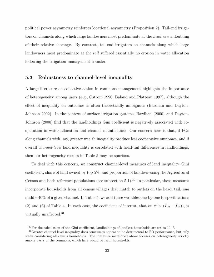
political power asymmetry reinforces locational asymmetry (Proposition 2). Tail-end irriga-

tors on channels along which large landowners most predominate at the head saw a doubling

of their relative shortage. By contrast, tail-end irrigators on channels along which large

landowners most predominate at the tail suffered essentially no erosion in water allocation

following the irrigation management transfer.

5.3 Robustness to channel-level inequality

A large literature on collective action in commons management highlights the importance

of heterogeneity among users (e.g., Ostrom 1990; Baland and Platteau 1997), although the

effect of inequality on outcomes is often theoretically ambiguous (Bardhan and Dayton-

Johnson 2002). In the context of surface irrigation systems, Bardhan (2000) and Dayton-

Johnson (2000) find that the landholdings Gini coefficient is negatively associated with co-

operation in water allocation and channel maintenance. Our concern here is that, if FOs

along channels with, say, greater wealth inequality produce less cooperative outcomes, and if

overall channel-level land inequality is correlated with head-tail differences in landholdings,

then our heterogeneity results in Table 5 may be spurious.

To deal with this concern, we construct channel-level measures of land inequality–Gini

coefficient, share of land owned by top 5%, and proportion of landless–using the Agricultural

Census and both reference populations (see subsection 5.1).30 In particular, these measures

incorporate households from all census villages that match to outlets on the head, tail, and

middle 40% of a given channel. In Table 5, we add these variables one-by-one to specifications

(2) and (6) of Table 4. In each case, the coefficient of interest, that on τ 1 × (LH − LT )), is

virtually unaffected.31

30For the calculation of the Gini coefficient, landholdings of landless households are set to 10−8.31Greater channel level inequality does sometimes appear to be detrimental to FO performance, but only

when considering all census households. The literature mentioned above focuses on heterogeneity strictlyamong users of the commons, which here would be farm households.

33

Table 5: Influence Asymmetry–Robustness to Channel-level Inequality

Census Farm Households All Census Households

Gini Top 5% share Landless prop. Gini Top 5% share Landless prop.

τ 1 0.0571 0.0159 0.0515*** -0.0898 0.00624 -0.0128(0.0581) (0.0342) (0.0156) (0.0687) (0.0364) (0.0274)

τ 1 × (LH − LT ) 0.00519*** 0.00499*** 0.00519*** 0.00932*** 0.00917*** 0.00939***(0.00191) (0.00192) (0.00194) (0.00305) (0.00301) (0.00302)

τ 1 × inequality -0.00396 0.0719 0.0206 0.189** 0.0810 0.146***(0.0911) (0.0596) (0.0659) (0.0868) (0.0546) (0.0511)

R2 0.571 0.571 0.571 0.570 0.570 0.570No. of Obs. 586,417 586,417 586,417 602,425 602,425 602,425No. of clusters 892 892 892 909 909 909No. of FOs 247 247 247 252 252 252

Notes: Robust standard errors in parentheses (*** p<0.01, ** p<0.05, * p<0.1), clustered on FO/distributary. Allspecifications use spatial matching with 60 km buffer. Dependent variable is tail shortage Y = DPRH − DPRT .Channel-years in 2nd FO tenure dropped. All specifications include controls for log(CV) of weekly discharge, channelfixed effects, Circle-specific time trends, and buffer-year fixed effects. Lj denotes mean land ownership at position jof channel computed over census farm households (cols 2-4) or all census households (cols 5-7); τ1 is indicator for firstFO tenure.

6 Conclusion

How a shift in resource control from centralized bureaucracy to local government affects

allocations of publicly provided goods has been an empirical terra incognita. It is worth

reiterating why this is so: natural experiments in decentralization are extremely rare, rarer

still in contexts where rent-seeking (or, rather, the consequences thereof) can be objectively

measured. The devolution of irrigation management in Pakistan’s Indus basin combined

with an extensive water discharge database provides just such a felicitous circumstance.

We have compared changes in water discharge along channels whose management was

taken over by locally elected farmer organizations (FOs) to changes that occurred in channels

that remained centrally managed. Water theft increased by more in the former case, leading

to a large redistribution of wealth. That decentralization also increased water theft by more

along channels with a greater preponderance of large landowners at the head suggests that

investment in de facto political power (borrowing the terminology of Acemoglu and Robinson

2008) can more than offset changes in de jure political power brought about by institutional

34

reform. Here, as our theoretical model indicates, decentralization shifts the lobbying arena

from the upper-tier of the bureaucratic hierarchy to the communal governance structure and

thereby enhances rent-seeking.

While our evidence is not favorable to the decentralization effort in the Indus basin

inasmuch as it did not deliver on its promise of a more equitable (and efficient) distribution

of canal water, it would be premature to throw out the reform baby with the bathwater.

Successful decentralization would likely involve directly addressing power asymmetries along

the irrigation system, such as by giving tail-enders exclusive control over FOs.32 In terms of

the model, this policy would make it more likely that the efficient allocation is implemented.

Tail-enders would have every incentive to enforce the warabandi system, while head-end

influence within the FO would be minimized. More generally, as Mansuri and Rao (2013)

argue, state support, both in setting and in enforcing the rules of the game, is a key ingredient

for effective local governance.

32Merely establishing reservations whereby each FO must have a certain number of members or officersrepresenting tail outlets may not be enough. In our data, a reasonable proportion of FO presidents (20%) andof the four-member FO management committee (18% on average) own land at the tail. In these cases, tail-enders’ interests are nominally represented in the FO. However, analysis similar to that in Table 4 (availablefrom the authors upon request) reveals no significant difference in decentralization outcomes between FOswith and without tail representation. To be sure, caution must be exercised in interpreting these results aswe do not understand why some FOs have officers with tail-holdings and others do not. Nevertheless, takenon their own terms, these finding do not support a partial reservation for tail-enders.

35

References

[1] Acemoglu, D., & Robinson, J. (2008). Persistence of Power, Elites, and Institutions.

American Economic Review, 98(1), 267-293.

[2] Alatas, V., Banerjee, A., Hanna, R., Olken, B. A., Purnamasari, R., & Wai-Poi, M.

(2013). Does elite capture matter? Local elites and targeted welfare programs in In-

donesia (No. w18798). National Bureau of Economic Research.

[3] Anderson, S., Francois, P., & Kotwal, A. (2015). Clientelism in Indian villages. American

Economic Review, 105(6), 1780-1816.

[4] Baland, J. M., & Platteau, J. P. (1997). Wealth inequality and efficiency in the commons

Part I: the unregulated case. Oxford Economic Papers, 49(4), 451-482.

[5] Baland, J. M., & Robinson, J. A. (2008). Land and power: Theory and evidence from

Chile. American Economic Review, 98(5), 1737-1765.

[6] Bardhan, P. (2000). Irrigation and cooperation: An empirical analysis of 48 irrigation

communities in South India. Economic Development and cultural change, 48(4), 847-

865.

[7] Bardhan, P., & Dayton-Johnson, J. (2002). Unequal irrigators: heterogeneity and com-

mons management in large-scale multivariate research. The drama of the commons,

87-112.

[8] Bardhan, P., & Mookherjee, D. (2006a). Decentralisation and accountability in infras-

tructure delivery in developing countries. Economic Journal, 116(508), 101-127.

[9] Bardhan, P., & Mookherjee, D. (2006b). Decentralization, corruption and government

accountability. International handbook on the economics of corruption, 6, 161-188.

36

[10] Bardhan, P., & Mookherjee, D. (2006). Pro-poor targeting and accountability of local

governments in West Bengal. Journal of development Economics, 79(2), 303-327.

[11] Bandaragoda, D. J., & ur Rehman, S. (1995). Warabandi in Pakistan’s canal irrigation

systems: Widening gap between theory and practice. No. 7. IWMI.

[12] Basurto, P., Dupas, P., & Robinson, J. (2015). Decentralization and efficiency of subsidy

targeting: Evidence from chiefs in rural Malawi. Unpublished, Stanford University.

[13] Beath, A., Christia, F., & Enikolopov, R. (2017). Direct democracy and resource allo-

cation: Experimental evidence from Afghanistan. Journal of Development Economics,

124, 199-213.

[14] Bromley, D. W., Taylor, D. C., & Parker, D. E. (1980). Water reform and economic

development: institutional aspects of water management in the developing countries.

Economic Development and Cultural Change, 365-387.

[15] Chakravorty, U., & Roumasset, J. (1991). Efficient spatial allocation of irrigation water.

American Journal of Agricultural Economics, 73(1), 165-173.

[16] Chambers, R. (1988). Managing canal irrigation: Practical analysis from south Asia.

New Delhi: Oxford.

[17] Dayton-Johnson, J. (2000). Determinants of collective action on the local commons: a

model with evidence from Mexico. Journal of Development Economics, 62(1), 181-208.

[18] Fan, C. S., Lin, C., & Treisman, D. (2009). Political decentralization and corruption:

Evidence from around the world. Journal of Public Economics, 93(1), 14-34.

[19] Guimaraes, P. and P. Portugal (2010). A Simple Feasible Alternative Procedure to

Estimate Models with High-Dimensional Fixed Effects, Stata Journal, 10(4), 628-649.

37

[20] Holmes, T. J. (1998). The effect of state policies on the location of manufacturing:

Evidence from state borders. Journal of Political Economy, 106(4), 667-705.

[21] Hoffman, V., P. Jakiela, M. Kremer, and R. Sheely (2017). There is no place like home:

Theory and evidence on decentralization and politician preferences. Unpublished.

[22] Jacoby, H. & Mansuri, G. (2017). Misgoverning the Commons: Corruption and Rent-

seeking in Pakistan’s Indus Basin. World Bank, Washington DC.

[23] Mansuri, G., and Rao, V. (2013). Localizing development: Does participation work?.

World Bank Publications.

[24] Mookherjee, D. (2015). Political decentralization. Annual Review of Economics 7, no.

1 (2015): 231-249.

[25] Meinzen-Dick, R. (2007). Beyond panaceas in water institutions. Proceedings of the

National Academy of Sciences, 104(39), 15200-15205.

[26] Moore, M. (1989). The fruits and fallacies of neoliberalism: the case of irrigation policy.

World Development, 17(11), 1733-1750.

[27] Nitzan, S. (1994). Modelling rent-seeking contests. European Journal of Political Econ-

omy 10, no. 1: 41-60.

[28] Ostrom, E. (1990). Governing the Commons: The Evolution of Institutions for Collec-

tive Action. New York: Cambridge University Press.

[29] Ostrom, E. & Gardner, R. (1993). Coping with asymmetries in the commons: self-

governing irrigation systems can work. Journal of Economic Perspectives, 7(4), 93-112.

[30] Rijsberman, F. R. (2008). Water for food: corruption in irrigation systems. Global

Corruption Report 2008, P. 67-84.

38

[31] Rinaudo, J. D., Strosser, P., & Thoyer, S. (2000). Distributing water or rents? Ex-

amples from a public irrigation system in Pakistan. Canadian Journal of Development

Studies/Revue canadienne d’etudes du developpement, 21(1):113-139.

[32] Rinaudo, J. D. (2002). Corruption and allocation of water: the case of public irrigation

in Pakistan. Water Policy, 4(5), 405-422.

[33] Sampath, R. K. (1992). Issues in irrigation pricing in developing countries. World De-

velopment, 20(7), 967-977.

[34] Tullock, G. (1980). Efficient rent-seeking. In Buchanan, J.; Tollison, R.; & Tullock, G.,

Toward a theory of the rent-seeking society, pp. 97-112.

[35] Van Waijjen, E. G., Hart, W. W. H., Kuper, M. & Brouwer, R. (1997). ”Using a

hydro-dynamic flow model to plan maintenance activities and improve irrigation water

distribution: application to the Fordwah distributary in Punjab, Pakistan.” Irrigation

and Drainage Systems 11, no. 4: 367-386.

[36] Vermillion, D. L. (1997). Impacts of irrigation management transfer: A review of the

evidence. Sri Lanka: International Irrigation Management Institute.

[37] Wade, R. (1982). The system of administrative and political corruption: Canal irrigation

in south India, J. of Development Studies, 18(3): 287-328.

[38] World Bank (2004) World Development Report 2004: Making Services Work for Poor

People. Washington, DC: World Bank.

39

Appendix

A Proofs

The following results hold at θ = 1, which is to say at the mean of relative influence:

Lemma 1. bF < bB.

Proof. The FOC for the bureaucratic official is V ′B(bB) = 0 (the SOC V ′′

B < 0 is always

satisfied) and the FOC for the FO official is V ′B(bF ) + u′(bF ) = 0. Since equilibrium efforts

are ej = P (1− P )∆j, we have eH + eT = P (1− P )(∆H + ∆T ) = ∆H∆T/(∆H + ∆T ) at

θ = 1. Thus,

u′(bB) =U ′(·)∆2

T∆′H

(∆H + ∆T )2< 0

since ∆′H(b) = −n. It follows that V ′

B(bF ) > V ′B(bB), which, by V ′′

B < 0,⇒ bF < bB.

Proof of Proposition 1: We have TS(br) = TSr = P (br)w, and Taylor expansion

TS(bF ) ≈ TS(bB) + TS ′(bB)(bF − bB).

Since P ′(br) < 0⇒ TS ′(bB) < 0, lemma 1 ⇒ TSF > TSB.

Proof of Proposition 2: We have Taylor expansion

TSθ(bF ) ≈ TSθ(bB) + TSθb(bB)(bF − bB).

where subscripts denote partial derivatives and TSθb(bB) = Pθb(bB)w. Next,

Pθb =

[P

b+ Pb

]bθb− Pθ

P.

Evaluated at bB, the expression in square brackets is proportional to V ′B(bB) and thus

vanishes. Since Pθ > 0, TSθb(bB) < 0, which, with lemma 1, proves the result.

40

B Additional Figures and Tables

Figure B.1: Indus Basin irrigation system in Punjab

41

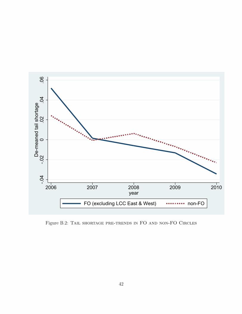
-.04

-.02

0.0

2.0

4.0

6D

e-m

eane

d ta

il sh

orta

ge

2006 2007 2008 2009 2010year

FO (excluding LCC East & West) non-FO

Figure B.2: Tail shortage pre-trends in FO and non-FO Circles

42

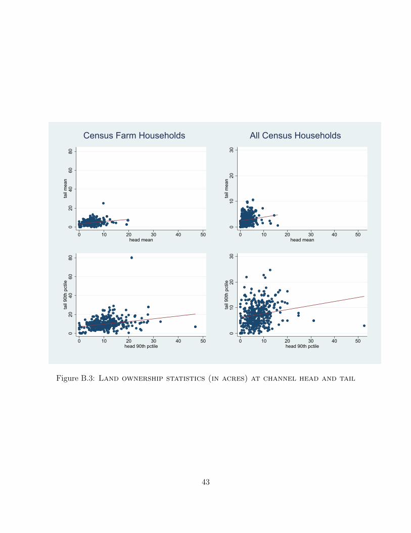
020

4060

80ta

il m

ean

0 10 20 30 40 50head mean

020

4060

80ta

il 90

th p

ctile

0 10 20 30 40 50head 90th pctile

Census Farm Households

010

2030

tail

mea

n

0 10 20 30 40 50head mean

010

2030

tail

90th

pct

ile

0 10 20 30 40 50head 90th pctile

All Census Households

Figure B.3: Land ownership statistics (in acres) at channel head and tail

43

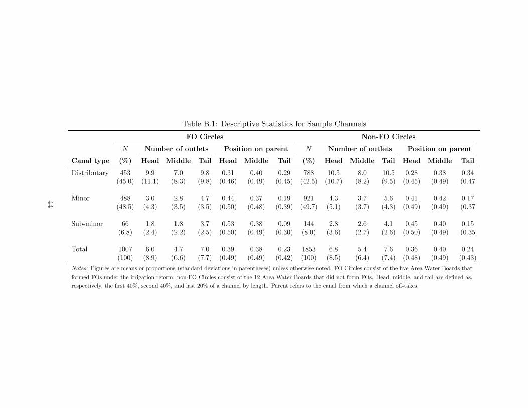
Table B.1: Descriptive Statistics for Sample Channels

FO Circles Non-FO Circles

N Number of outlets Position on parent N Number of outlets Position on parent

Canal type (%) Head Middle Tail Head Middle Tail (%) Head Middle Tail Head Middle Tail

Distributary 453 9.9 7.0 9.8 0.31 0.40 0.29 788 10.5 8.0 10.5 0.28 0.38 0.34(45.0) (11.1) (8.3) (9.8) (0.46) (0.49) (0.45) (42.5) (10.7) (8.2) (9.5) (0.45) (0.49) (0.47

Minor 488 3.0 2.8 4.7 0.44 0.37 0.19 921 4.3 3.7 5.6 0.41 0.42 0.17(48.5) (4.3) (3.5) (3.5) (0.50) (0.48) (0.39) (49.7) (5.1) (3.7) (4.3) (0.49) (0.49) (0.37

Sub-minor 66 1.8 1.8 3.7 0.53 0.38 0.09 144 2.8 2.6 4.1 0.45 0.40 0.15(6.8) (2.4) (2.2) (2.5) (0.50) (0.49) (0.30) (8.0) (3.6) (2.7) (2.6) (0.50) (0.49) (0.35

Total 1007 6.0 4.7 7.0 0.39 0.38 0.23 1853 6.8 5.4 7.6 0.36 0.40 0.24(100) (8.9) (6.6) (7.7) (0.49) (0.49) (0.42) (100) (8.5) (6.4) (7.4) (0.48) (0.49) (0.43)

Notes: Figures are means or proportions (standard deviations in parentheses) unless otherwise noted. FO Circles consist of the five Area Water Boards that

formed FOs under the irrigation reform; non-FO Circles consist of the 12 Area Water Boards that did not form FOs. Head, middle, and tail are defined as,

respectively, the first 40%, second 40%, and last 20% of a channel by length. Parent refers to the canal from which a channel off-takes.

44

Table B.2: Influence Asymmetry and FO Performance – Alternative Estimates

Census Farm Households All Census Households

Mean 90th percentile Mean 90th percentile

τ (α1 = α2) 0.0453** 0.0505*** 0.0487*** 0.0507*** 0.0569*** 0.0528*** 0.0584*** 0.0526***(0.0189) (0.00973) (0.0173) (0.00972) (0.0165) (0.00953) (0.0183) (0.00957)

τ × LH (δH) 0.00494** 0.00167 0.00728** 0.00289**(0.00208) (0.00105) (0.00294) (0.00124)

τ × LT (δT ) -0.00385 -0.00148 -0.00874** -0.00368*(0.00298) (0.00102) (0.00437) (0.00193)

τ × (LH − LT ) 0.00446** 0.00157** 0.00788*** 0.00319***(0.00183) (0.000783) (0.00264) (0.00108)

p-value δH = −δT 0.752 - 0.888 - 0.767 - 0.722 -

R2 0.571 0.571 0.571 0.571 0.570 0.570 0.570 0.570No. of Obs. 586,679 586,679 586,679 586,679 602,703 602,703 602,703 602,703No. of clusters 892 892 892 892 909 909 909 909No. of FOs 247 247 247 247 252 252 252 252

Notes: Robust standard errors in parentheses (*** p<0.01, ** p<0.05, * p<0.1), clustered on FO/distributary. All specifications use spatialmatching with 60 km buffer. Channel-years in 2nd tenure included with 1st and 2nd tenure effects constrained to be equal (τ is indicator for FOtenure, either 1st or 2nd). Dependent variable is tail shortage Y = DPRH −DPRT . All specifications include controls for log(CV) of weeklydischarge, channel fixed effects, Circle-specific time trends, and buffer-year fixed effects. Lj denotes mean or 90th percentile of land ownershipdistribution at position j of channel computed over census farm households (cols 2-5) or all census households (cols 6-9).

45