Embed Size (px)
Citation preview
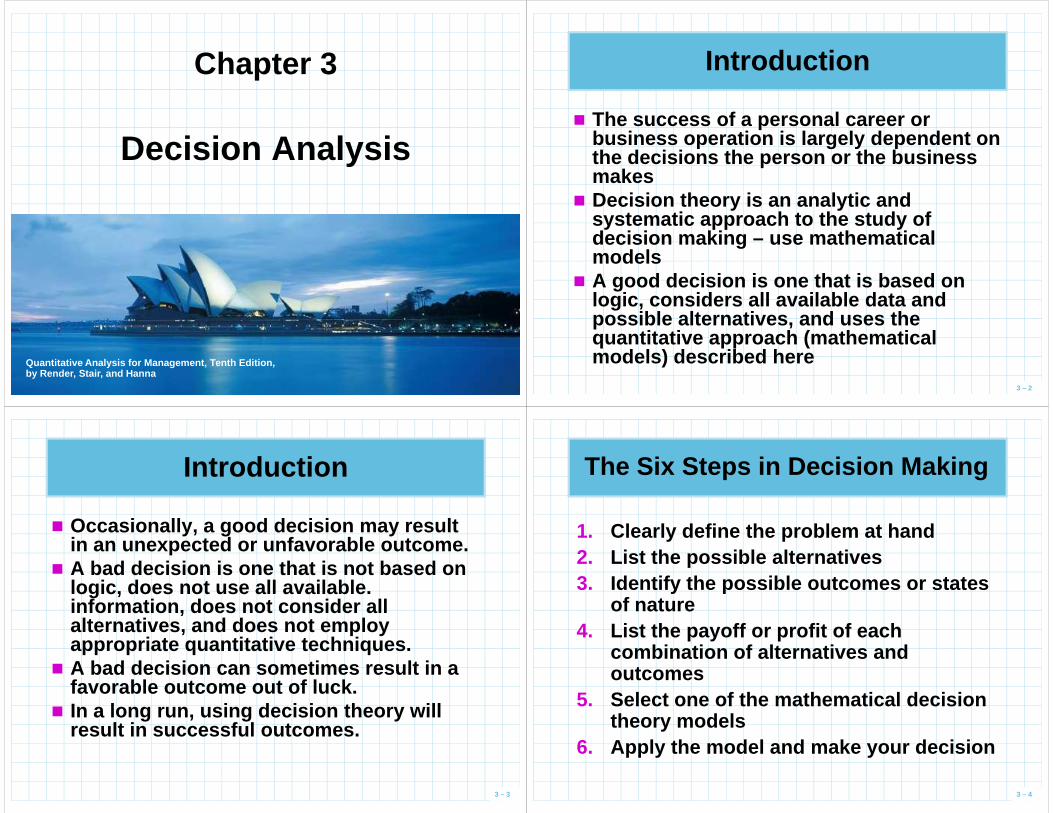
Chapter 3
Decision Analysis
© 2008 Prentice-Hall, Inc.Quantitative Analysis for Management , Tenth Edition ,by Render, Stair, and Hanna
Introduction
� The success of a personal career or business operation is largely dependent on the decisions the person or the business makes
� Decision theory is an analytic and
3 – 2
� Decision theory is an analytic and systematic approach to the study of decision making – use mathematical models
� A good decision is one that is based on logic, considers all available data and possible alternatives, and uses the quantitative approach (mathematical models) described here
Introduction
� Occasionally, a good decision may result in an unexpected or unfavorable outcome.
� A bad decision is one that is not based on logic, does not use all available. information, does not consider all
3 – 3
information, does not consider all alternatives, and does not employ appropriate quantitative techniques.
� A bad decision can sometimes result in a favorable outcome out of luck.
� In a long run, using decision theory will result in successful outcomes.
The Six Steps in Decision Making
1. Clearly define the problem at hand2. List the possible alternatives3. Identify the possible outcomes or states
of nature
3 – 4
of nature4. List the payoff or profit of each
combination of alternatives and outcomes
5. Select one of the mathematical decision theory models
6. Apply the model and make your decision
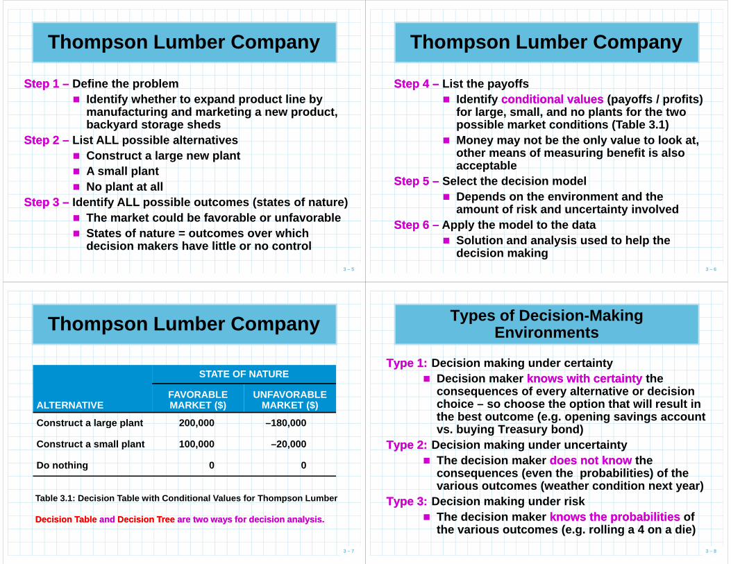
Thompson Lumber Company
Step 1 Step 1 –– Define the problem� Identify whether to expand product line by
manufacturing and marketing a new product, backyard storage sheds
Step 2 Step 2 –– List ALL possible alternatives
3 – 5
Step 2 Step 2 –– List ALL possible alternatives � Construct a large new plant� A small plant� No plant at all
Step 3 Step 3 –– Identify ALL possible outcomes (states of nature)� The market could be favorable or unfavorable� States of nature = outcomes over which
decision makers have little or no control
Thompson Lumber Company
Step 4 Step 4 –– List the payoffs� Identify conditional valuesconditional values (payoffs / profits)
for large, small, and no plants for the two possible market conditions (Table 3.1)
� Money may not be the only value to look at,
3 – 6
� Money may not be the only value to look at, other means of measuring benefit is also acceptable
Step 5 Step 5 –– Select the decision model� Depends on the environment and the
amount of risk and uncertainty involvedStep 6 Step 6 –– Apply the model to the data
� Solution and analysis used to help the decision making
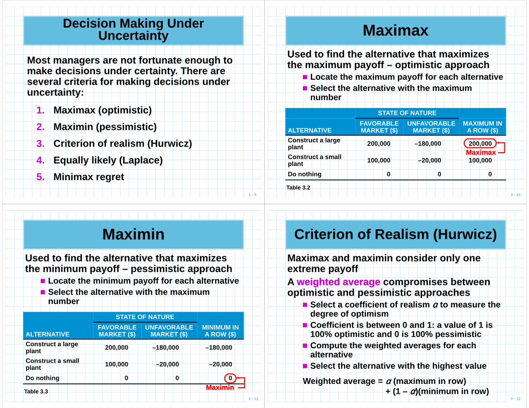
Thompson Lumber Company
STATE OF NATURE
ALTERNATIVEFAVORABLE MARKET ($)
UNFAVORABLE MARKET ($)
Construct a large plant 200,000 –180,000
3 – 7
Construct a large plant 200,000 –180,000
Construct a small plant 100,000 –20,000
Do nothing 0 0
Table 3.1: Decision Table with Conditional Values f or Thompson Lumber
Decision Table Decision Table andand Decision Tree Decision Tree are two ways for decision analysis.are two ways for decision analysis.
Types of Decision-Making Environments
Type 1:Type 1: Decision making under certainty� Decision maker knows with certaintyknows with certainty the
consequences of every alternative or decision choice – so choose the option that will result in the best outcome (e.g. opening savings account vs. buying Treasury bond)
3 – 8
vs. buying Treasury bond)Type 2:Type 2: Decision making under uncertainty
� The decision maker does not knowdoes not know the consequences (even the probabilities) of the various outcomes (weather condition next year)
Type 3:Type 3: Decision making under risk� The decision maker knows the probabilitiesknows the probabilities of
the various outcomes (e.g. rolling a 4 on a die)
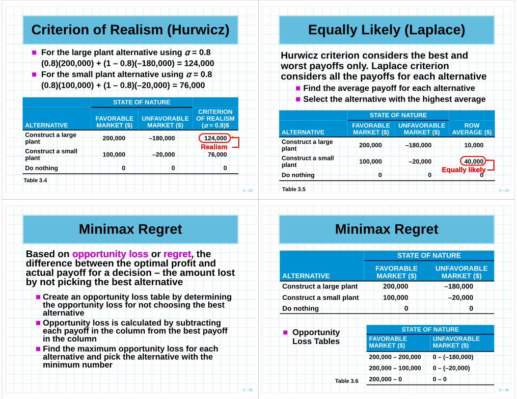
Decision Making Under Uncertainty
Most managers are not fortunate enough to make decisions under certainty. There are several criteria for making decisions under uncertainty:
3 – 9
1. Maximax (optimistic)
2. Maximin (pessimistic)
3. Criterion of realism (Hurwicz)
4. Equally likely (Laplace)
5. Minimax regret
MaximaxUsed to find the alternative that maximizes the maximum payoff – optimistic approach
� Locate the maximum payoff for each alternative� Select the alternative with the maximum
number
3 – 10
STATE OF NATURE
ALTERNATIVEFAVORABLE MARKET ($)
UNFAVORABLE MARKET ($)
MAXIMUM IN A ROW ($)
Construct a large plant 200,000 –180,000 200,000
Construct a small plant 100,000 –20,000 100,000
Do nothing 0 0 0
Table 3.2
MaximaxMaximax
MaximinUsed to find the alternative that maximizes the minimum payoff – pessimistic approach
� Locate the minimum payoff for each alternative� Select the alternative with the maximum
number
3 – 11
STATE OF NATURE
ALTERNATIVEFAVORABLE MARKET ($)
UNFAVORABLE MARKET ($)
MINIMUM IN A ROW ($)
Construct a large plant 200,000 –180,000 –180,000
Construct a small plant 100,000 –20,000 –20,000
Do nothing 0 0 0
Table 3.3MaximinMaximin
Criterion of Realism (Hurwicz)
Maximax and maximin consider only one extreme payoffA weighted averageweighted average compromises between optimistic and pessimistic approaches
� Select a coefficient of realism αααα to measure the
3 – 12
� Select a coefficient of realism αααα to measure the degree of optimism
� Coefficient is between 0 and 1: a value of 1 is 100% optimistic and 0 is 100% pessimistic
� Compute the weighted averages for each alternative
� Select the alternative with the highest value
Weighted average = αααα (maximum in row) + (1 – αααα)(minimum in row)
Criterion of Realism (Hurwicz)
� For the large plant alternative using αααα = 0.8(0.8)(200,000) + (1 – 0.8)(–180,000) = 124,000
� For the small plant alternative using αααα = 0.8 (0.8)(100,000) + (1 – 0.8)(–20,000) = 76,000
STATE OF NATURE
3 – 13
STATE OF NATURE
ALTERNATIVEFAVORABLE MARKET ($)
UNFAVORABLE MARKET ($)
CRITERION OF REALISM
(αααα = 0.8)$
Construct a large plant 200,000 –180,000 124,000
Construct a small plant 100,000 –20,000 76,000
Do nothing 0 0 0
Table 3.4
RealismRealism
Equally Likely (Laplace)
Hurwicz criterion considers the best and worst payoffs only. Laplace criterion considers all the payoffs for each alternative
� Find the average payoff for each alternative� Select the alternative with the highest average
3 – 14
� Select the alternative with the highest average
STATE OF NATURE
ALTERNATIVEFAVORABLE MARKET ($)
UNFAVORABLE MARKET ($)
ROW AVERAGE ($)
Construct a large plant 200,000 –180,000 10,000
Construct a small plant 100,000 –20,000 40,000
Do nothing 0 0 0
Table 3.5
Equally likelyEqually likely
Minimax Regret
Based on opportunity lossopportunity loss or regretregret , the difference between the optimal profit and actual payoff for a decision – the amount lost by not picking the best alternative
� Create an opportunity loss table by determining
3 – 15
� Create an opportunity loss table by determining the opportunity loss for not choosing the best alternative
� Opportunity loss is calculated by subtracting each payoff in the column from the best payoff in the column
� Find the maximum opportunity loss for each alternative and pick the alternative with the minimum number
Minimax Regret
STATE OF NATURE
ALTERNATIVEFAVORABLE MARKET ($)
UNFAVORABLE MARKET ($)
Construct a large plant 200,000 –180,000
Construct a small plant 100,000 –20,000
3 – 16
STATE OF NATURE
FAVORABLE MARKET ($)
UNFAVORABLE MARKET ($)
200,000 – 200,000 0 – (–180,000)
200,000 – 100,000 0 – (–20,000)
200,000 – 0 0 – 0Table 3.6
� Opportunity Loss Tables
Construct a small plant 100,000 –20,000
Do nothing 0 0
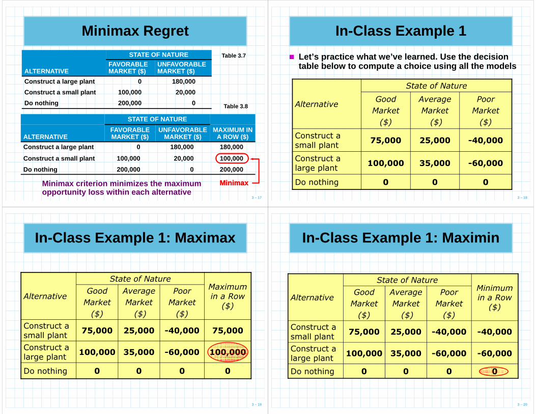
Minimax Regret
Table 3.8
Table 3.7STATE OF NATURE
ALTERNATIVEFAVORABLE MARKET ($)
UNFAVORABLE MARKET ($)
Construct a large plant 0 180,000
Construct a small plant 100,000 20,000
Do nothing 200,000 0
3 – 17
Table 3.8
STATE OF NATURE
ALTERNATIVEFAVORABLE MARKET ($)
UNFAVORABLE MARKET ($)
MAXIMUM IN A ROW ($)
Construct a large plant 0 180,000 180,000
Construct a small plant 100,000 20,000 100,000
Do nothing 200,000 0 200,000
MinimaxMinimaxMinimax criterion minimizes the maximum opportunity loss within each alternative
Do nothing 200,000 0
� Let’s practice what we’ve learned. Use the decision table below to compute a choice using all the model s
In-Class Example 1
Alternative
State of Nature
Good Average Poor
3 – 18
AlternativeMarket
($)
Market
($)
Market
($)
Construct a small plant
75,000 25,000 -40,000
Construct a large plant
100,000 35,000 -60,000
Do nothing 0 0 0
In-Class Example 1: Maximax
Alternative
State of NatureMaximum in a Row
($)
Good
Market
($)
Average
Market
($)
Poor
Market
($)
3 – 19
($) ($) ($)
Construct a small plant
75,000 25,000 -40,000 75,000
Construct a large plant
100,000 35,000 -60,000 100,000
Do nothing 0 0 0 0
In-Class Example 1: Maximin
Alternative
State of NatureMinimum in a Row
($)
Good
Market
($)
Average
Market
($)
Poor
Market
($)
3 – 20
($)($) ($) ($)
Construct a small plant
75,000 25,000 -40,000 -40,000
Construct a large plant
100,000 35,000 -60,000 -60,000
Do nothing 0 0 0 0
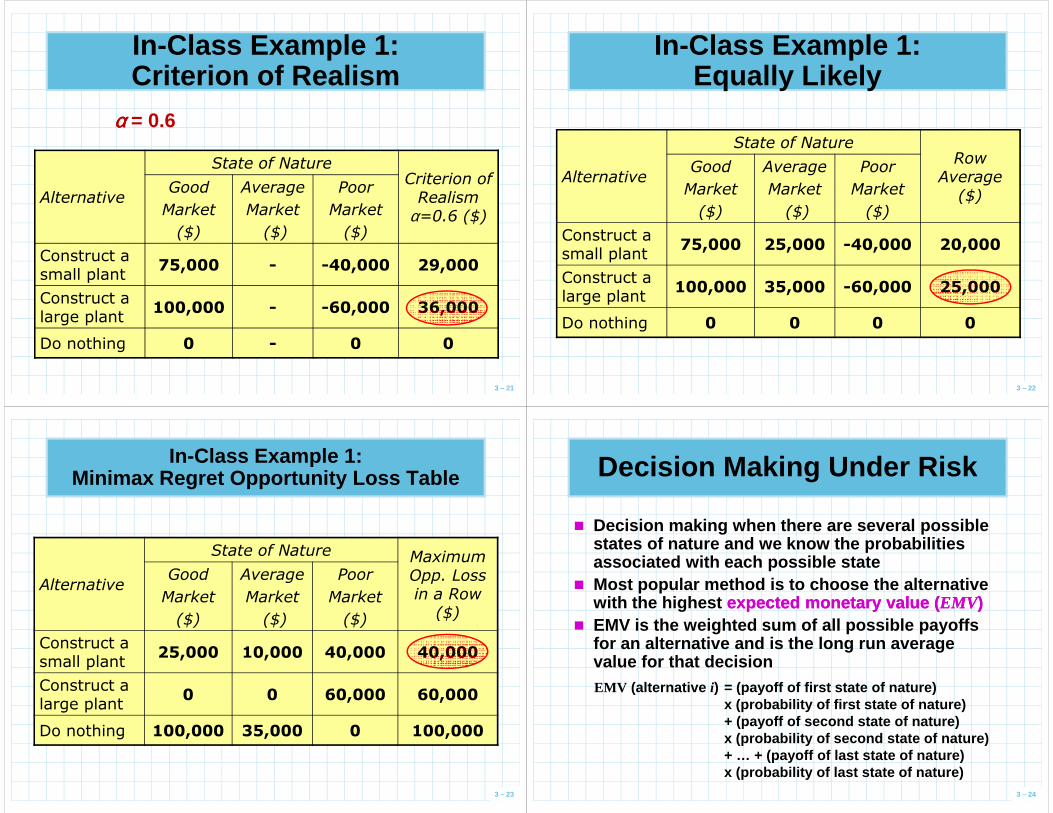
In-Class Example 1: Criterion of Realism
Alternative
State of NatureCriterion of
Realism Good
Market
Average
Market
Poor
Market
αααα = 0.6
3 – 21
Alternative Realism α=0.6 ($)Market
($)
Market
($)
Market
($)
Construct a small plant
75,000 - -40,000 29,000
Construct a large plant
100,000 - -60,000 36,000
Do nothing 0 - 0 0
In-Class Example 1: Equally Likely
Alternative
State of NatureRow
Average ($)
Good
Market
($)
Average
Market
($)
Poor
Market
($)
3 – 22
($)($) ($) ($)
Construct a small plant
75,000 25,000 -40,000 20,000
Construct a large plant
100,000 35,000 -60,000 25,000
Do nothing 0 0 0 0
Alternative
State of Nature Maximum Opp. Loss in a Row
($)
Good
Market
($)
Average
Market
($)
Poor
Market
($)
In-Class Example 1:Minimax Regret Opportunity Loss Table
3 – 23
($)($) ($) ($)
Construct a small plant
25,000 10,000 40,000 40,000
Construct a large plant
0 0 60,000 60,000
Do nothing 100,000 35,000 0 100,000
Decision Making Under Risk
� Decision making when there are several possible states of nature and we know the probabilities associated with each possible state
� Most popular method is to choose the alternative with the highest expected monetary value (expected monetary value ( EMVEMV) )
3 – 24
with the highest expected monetary value (expected monetary value ( EMVEMV) ) � EMV is the weighted sum of all possible payoffs
for an alternative and is the long run average value for that decisionEMV (alternative i) = (payoff of first state of nature)
x (probability of first state of nature)+ (payoff of second state of nature)x (probability of second state of nature)+ … + (payoff of last state of nature)x (probability of last state of nature)
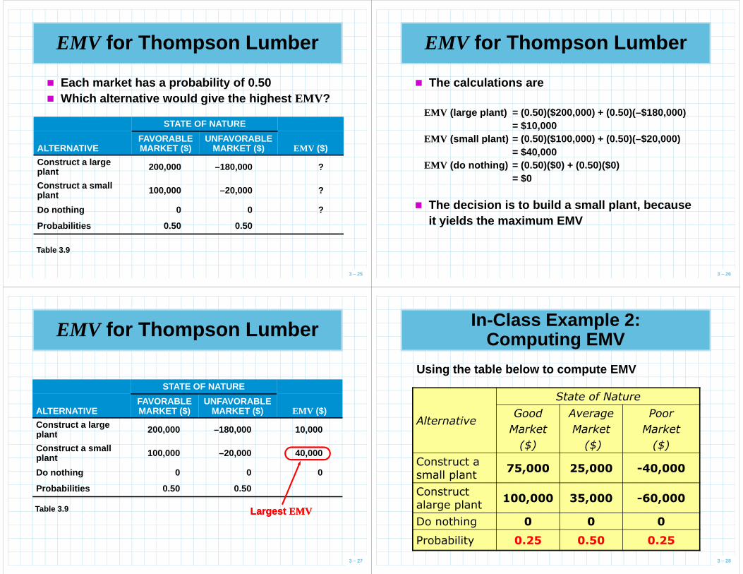
EMV for Thompson Lumber
STATE OF NATURE
ALTERNATIVEFAVORABLE MARKET ($)
UNFAVORABLE MARKET ($) EMV ($)
� Each market has a probability of 0.50� Which alternative would give the highest EMV ?
3 – 25
ALTERNATIVE MARKET ($) MARKET ($) EMV ($)
Construct a large plant 200,000 –180,000 ?
Construct a small plant 100,000 –20,000 ?
Do nothing 0 0 ?
Probabilities 0.50 0.50
Table 3.9
EMV for Thompson Lumber
� The calculations are
EMV (large plant) = (0.50)($200,000) + (0.50)(–$180,000)= $10,000
EMV (small plant) = (0.50)($100,000) + (0.50)(–$20,000)
3 – 26
EMV (small plant) = (0.50)($100,000) + (0.50)(–$20,000)= $40,000
EMV (do nothing) = (0.50)($0) + (0.50)($0)= $0
� The decision is to build a small plant, becauseit yields the maximum EMV
EMV for Thompson Lumber
STATE OF NATURE
ALTERNATIVEFAVORABLE MARKET ($)
UNFAVORABLE MARKET ($) EMV ($)
Construct a large plant 200,000 –180,000 10,000
3 – 27
plant 200,000 –180,000 10,000
Construct a small plant 100,000 –20,000 40,000
Do nothing 0 0 0
Probabilities 0.50 0.50
Table 3.9 Largest Largest EMVEMV
In-Class Example 2: Computing EMV
Alternative
State of Nature
Good
Market
Average
Market
Poor
Market
Using the table below to compute EMV
3 – 28
Market
($)
Market
($)
Market
($)
Construct a small plant
75,000 25,000 -40,000
Construct alarge plant
100,000 35,000 -60,000
Do nothing 0 0 0
Probability 0.25 0.50 0.25
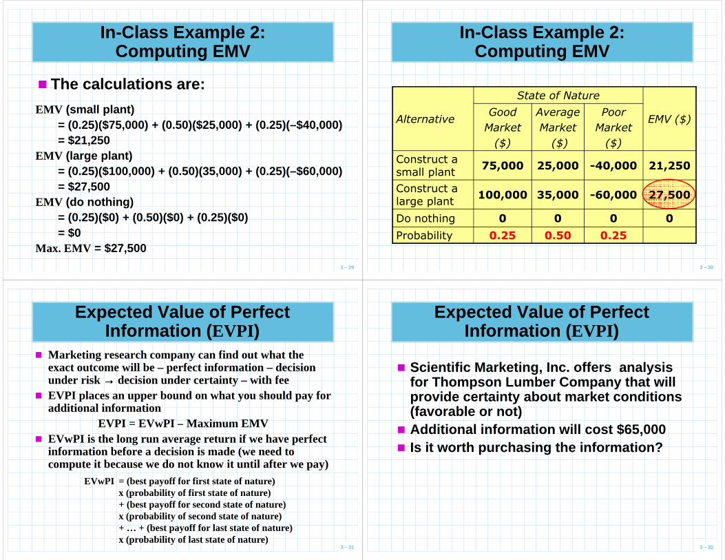
� The calculations are:
In-Class Example 2: Computing EMV
EMV (small plant)= (0.25)($75,000) + (0.50)($25,000) + (0.25)(–$40,000)= $21,250
3 – 29
= $21,250EMV (large plant)
= (0.25)($100,000) + (0.50)(35,000) + (0.25)(–$60,000)= $27,500
EMV (do nothing)= (0.25)($0) + (0.50)($0) + (0.25)($0) = $0
Max. EMV = $27,500
In-Class Example 2: Computing EMV
Alternative
State of Nature
EMV ($)Good
Market
($)
Average
Market
($)
Poor
Market
($)
3 – 30
($) ($) ($)
Construct a small plant
75,000 25,000 -40,000 21,250
Construct a large plant
100,000 35,000 -60,000 27,500
Do nothing 0 0 0 0
Probability 0.25 0.50 0.25
Expected Value of Perfect Information ( EVPI )
� Marketing research company can find out what the exact outcome will be – perfect information – decision under risk →→→→ decision under certainty – with fee
� EVPI places an upper bound on what you should pay for additional information
EVPI = EVwPI – Maximum EMV
3 – 31
EVPI = EVwPI – Maximum EMV� EVwPI is the long run average return if we have perfect
information before a decision is made (we need to compute it because we do not know it until after we pay)
EVwPI = (best payoff for first state of nature)x (probability of first state of nature)+ (best payoff for second state of nature)x (probability of second state of nature)+ … + (best payoff for last state of nature)x (probability of last state of nature)
Expected Value of Perfect Information ( EVPI )
� Scientific Marketing, Inc. offers analysis for Thompson Lumber Company that will provide certainty about market conditions (favorable or not)
3 – 32
� Additional information will cost $65,000� Is it worth purchasing the information?
Expected Value of Perfect Information ( EVPI )
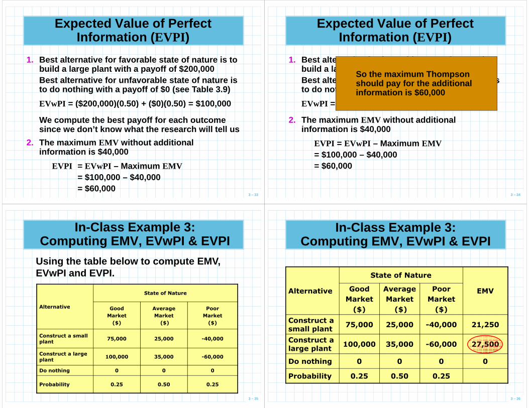
1. Best alternative for favorable state of nature is t o build a large plant with a payoff of $200,000Best alternative for unfavorable state of nature is to do nothing with a payoff of $0 (see Table 3.9)
EVwPI = ($200,000)(0.50) + ($0)(0.50) = $100,000
3 – 33
EVwPI = ($200,000)(0.50) + ($0)(0.50) = $100,000
We compute the best payoff for each outcome since we don’t know what the research will tell us
2. The maximum EMV without additional information is $40,000
EVPI = EVwPI – Maximum EMV= $100,000 – $40,000= $60,000
Expected Value of Perfect Information ( EVPI )
1. Best alternative for favorable state of nature is build a large plant with a payoff of $200,000Best alternative for unfavorable state of nature is to do nothing with a payoff of $0
EVwPI = ($200,000)(0.50) + ($0)(0.50) = $100,000
So the maximum Thompson should pay for the additional information is $60,000
3 – 34
EVwPI = ($200,000)(0.50) + ($0)(0.50) = $100,000
2. The maximum EMV without additional information is $40,000
EVPI = EVwPI – Maximum EMV= $100,000 – $40,000= $60,000
In-Class Example 3:Computing EMV, EVwPI & EVPI
Using the table below to compute EMV, EVwPI and EVPI.
Alternative
State of Nature
Good Average Poor
3 – 35
Alternative Good
Market
($)
Average
Market
($)
Poor
Market
($)
Construct a small plant
75,000 25,000 -40,000
Construct a large plant
100,000 35,000 -60,000
Do nothing 0 0 0
Probability 0.25 0.50 0.25
In-Class Example 3:Computing EMV, EVwPI & EVPI
Alternative
State of Nature
EMVGood
Market
($)
Average
Market
($)
Poor
Market
($)
3 – 36
($) ($) ($)
Construct a small plant
75,000 25,000 -40,000 21,250
Construct a large plant
100,000 35,000 -60,000 27,500
Do nothing 0 0 0 0
Probability 0.25 0.50 0.25
In-Class Example 3:Computing EMV, EVwPI & EVPI
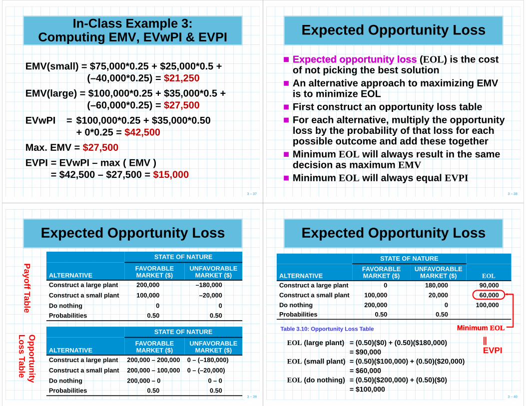
EMV(small) = $75,000*0.25 + $25,000*0.5 +(–40,000*0.25) = $21,250
EMV(large) = $100,000*0.25 + $35,000*0.5 +(–60,000*0.25) = $27,500
3 – 37
(–60,000*0.25) = $27,500
EVwPI = $100,000*0.25 + $35,000*0.50 + 0*0.25 = $42,500
Max. EMV = $27,500
EVPI = EVwPI – max ( EMV )= $42,500 – $27,500 = $15,000
Expected Opportunity Loss
�� Expected opportunity lossExpected opportunity loss (EOL ) is the cost of not picking the best solution
� An alternative approach to maximizing EMV is to minimize EOLFirst construct an opportunity loss table
3 – 38
� First construct an opportunity loss table� For each alternative, multiply the opportunity
loss by the probability of that loss for each possible outcome and add these together
� Minimum EOL will always result in the same decision as maximum EMV
� Minimum EOL will always equal EVPI
Expected Opportunity Loss
STATE OF NATURE
ALTERNATIVEFAVORABLE MARKET ($)
UNFAVORABLE MARKET ($)
Construct a large plant 200,000 –180,000
Construct a small plant 100,000 –20,000
Do nothing 0 0
Payoff Table
3 – 39
Do nothing 0 0
Probabilities 0.50 0.50
STATE OF NATURE
ALTERNATIVEFAVORABLE MARKET ($)
UNFAVORABLE MARKET ($)
Construct a large plant 200,000 – 200,000 0 – (–180,000 )
Construct a small plant 200,000 – 100,000 0 – (–20,000)
Do nothing 200,000 – 0 0 – 0
Probabilities 0.50 0.50
Payoff Table
Opportunity
Loss Table
Expected Opportunity Loss
STATE OF NATURE
ALTERNATIVEFAVORABLE MARKET ($)
UNFAVORABLE MARKET ($) EOL
Construct a large plant 0 180,000 90,000
Construct a small plant 100,000 20,000 60,000
Do nothing 200,000 0 100,000
3 – 40
EOL (large plant) = (0.50)($0) + (0.50)($180,000)= $90,000
EOL (small plant) = (0.50)($100,000) + (0.50)($20,000)= $60,000
EOL (do nothing) = (0.50)($200,000) + (0.50)($0)= $100,000
Table 3.10: Opportunity Loss Table
Do nothing 200,000 0 100,000Probabilities 0.50 0.50
Minimum Minimum EOLEOL
||||||||EVPI
Sensitivity Analysis
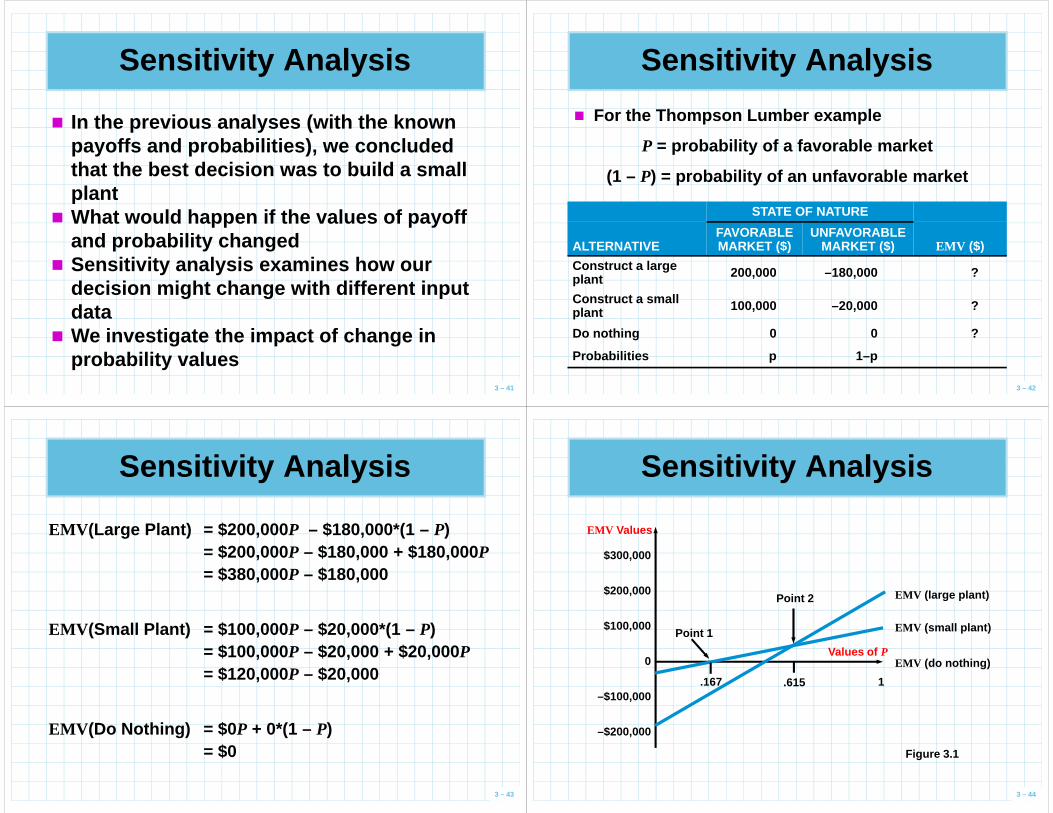
� In the previous analyses (with the known payoffs and probabilities), we concluded that the best decision was to build a small plant
3 – 41
plant� What would happen if the values of payoff
and probability changed � Sensitivity analysis examines how our
decision might change with different input data
� We investigate the impact of change in probability values
Sensitivity Analysis
� For the Thompson Lumber example
P = probability of a favorable market
(1 – P) = probability of an unfavorable market
3 – 42
STATE OF NATURE
ALTERNATIVEFAVORABLE MARKET ($)
UNFAVORABLE MARKET ($) EMV ($)
Construct a large plant 200,000 –180,000 ?
Construct a small plant 100,000 –20,000 ?
Do nothing 0 0 ?
Probabilities p 1–p
Sensitivity Analysis
EMV (Large Plant) = $200,000 P – $180,000*(1 – P)= $200,000P – $180,000 + $180,000P= $380,000P – $180,000
3 – 43
EMV (Small Plant) = $100,000 P – $20,000*(1 – P)= $100,000P – $20,000 + $20,000P= $120,000P – $20,000
EMV (Do Nothing) = $0 P + 0*(1 – P)= $0
Sensitivity Analysis
$300,000
$200,000
EMV Values
EMV (large plant)Point 2
3 – 44
$100,000
0
–$100,000
–$200,000
EMV (small plant)
EMV (do nothing)
Point 1
.167 .615 1
Values of P
Figure 3.1
Sensitivity Analysis
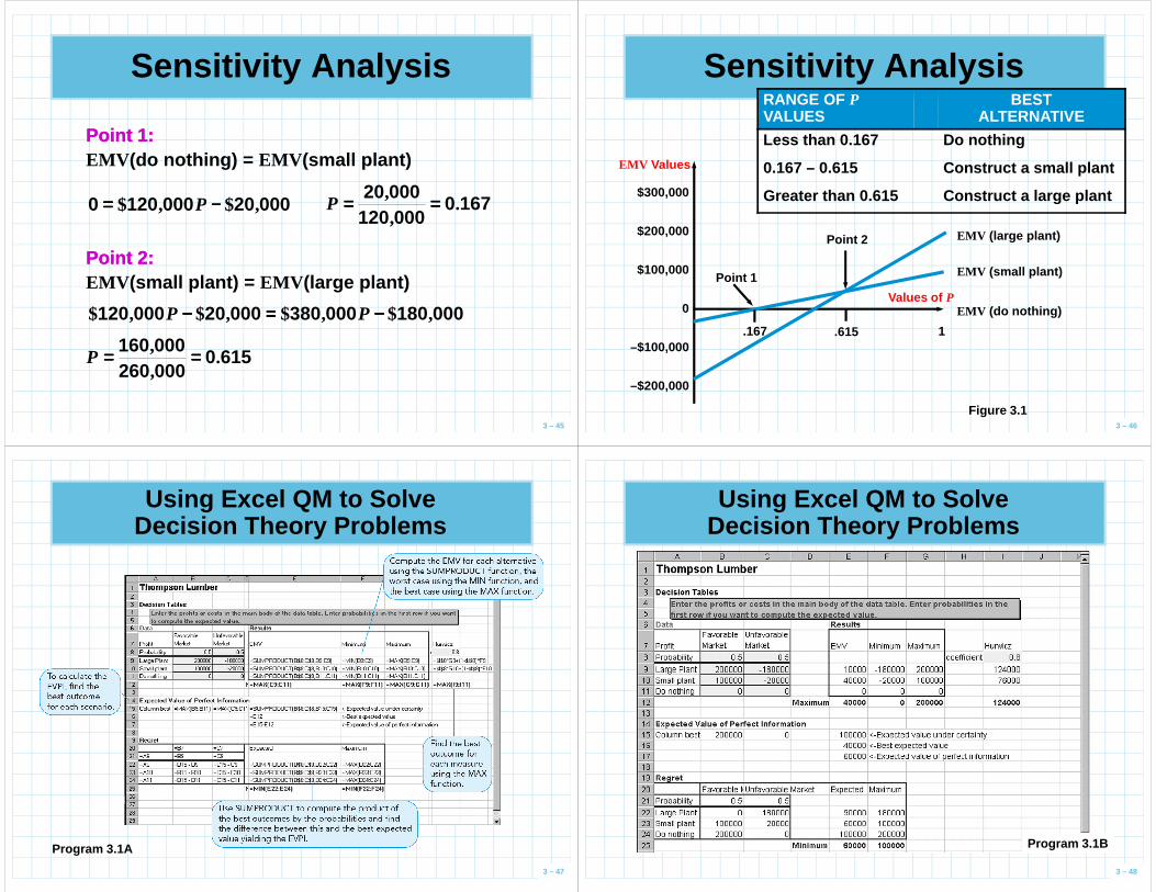
Point 1:Point 1:EMV (do nothing) = EMV (small plant)
000200001200 ,$,$ −−−−==== P 167000012000020
.,, ========P
3 – 45
000120,
00018000038000020000120 ,$,$,$,$ −−−−====−−−− PP
6150000260000160
.,, ========P
Point 2:Point 2:EMV (small plant) = EMV (large plant)
Sensitivity Analysis
$300,000
EMV Values
RANGE OF PVALUES
BEST ALTERNATIVE
Less than 0.167 Do nothing
0.167 – 0.615 Construct a small plant
Greater than 0.615 Construct a large plant
3 – 46
$200,000
$100,000
0
–$100,000
–$200,000
EMV (large plant)
EMV (small plant)
EMV (do nothing)
Point 1
Point 2
.167 .615 1
Values of P
Figure 3.1
Using Excel QM to Solve Decision Theory Problems
3 – 47
Program 3.1A
Using Excel QM to Solve Decision Theory Problems
3 – 48
Program 3.1B
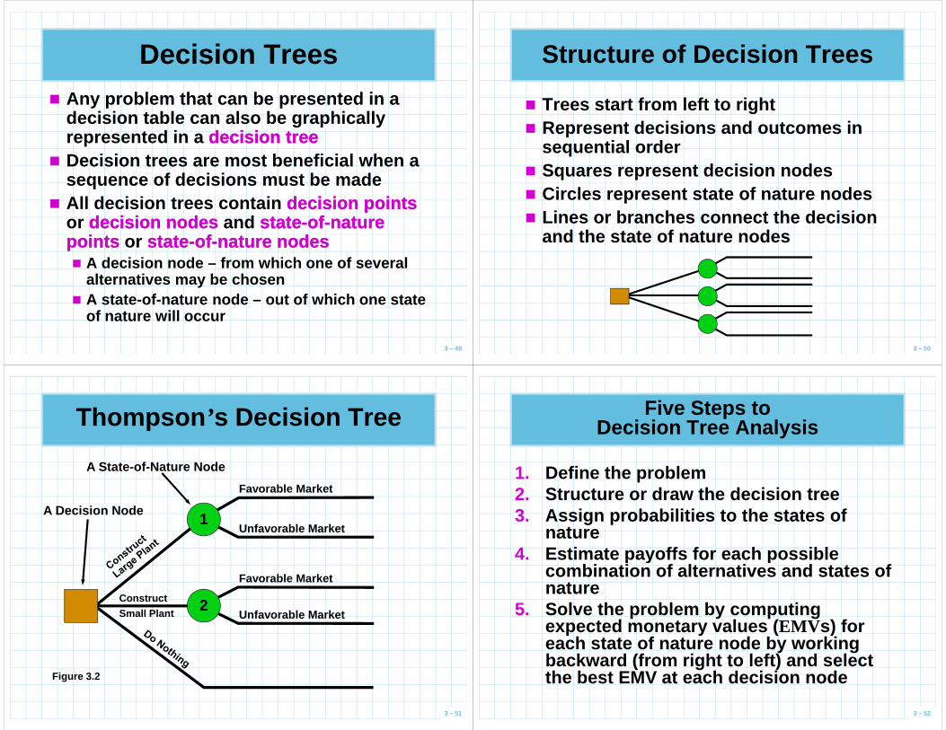
Decision Trees� Any problem that can be presented in a
decision table can also be graphically represented in a decision treedecision tree
� Decision trees are most beneficial when a sequence of decisions must be made
3 – 49
sequence of decisions must be made� All decision trees contain decision pointsdecision points
or decision nodesdecision nodes and statestate--ofof--nature nature pointspoints or statestate--ofof--nature nodesnature nodes� A decision node – from which one of several
alternatives may be chosen� A state-of-nature node – out of which one state
of nature will occur
Structure of Decision Trees
� Trees start from left to right� Represent decisions and outcomes in
sequential order� Squares represent decision nodes
3 – 50
� Circles represent state of nature nodes� Lines or branches connect the decision
and the state of nature nodes
Thompson ’s Decision Tree
Favorable Market
Unfavorable Market1
A Decision Node
A State-of-Nature Node
3 – 51
Favorable Market
Unfavorable MarketConstruct
Small Plant2
Figure 3.2
Five Steps toDecision Tree Analysis
1. Define the problem2. Structure or draw the decision tree3. Assign probabilities to the states of
nature4. Estimate payoffs for each possible
3 – 52
4. Estimate payoffs for each possible combination of alternatives and states of nature
5. Solve the problem by computing expected monetary values ( EMV s) for each state of nature node by working backward (from right to left) and select the best EMV at each decision node
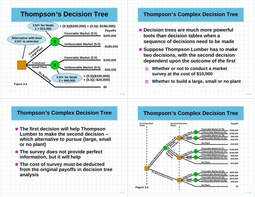
Thompson ’s Decision Tree
Favorable Market
Unfavorable Market1
Alternative with best EMV is selected
EMV for Node 1 = $10,000
= (0.5)($200,000) + (0.5)(–$180,000)Payoffs
$200,000
–$180,000
(0.5)
(0.5)
3 – 53
Favorable Market
Unfavorable MarketConstruct
Small Plant2
Figure 3.3
EMV for Node 2 = $40,000
= (0.5)($100,000) + (0.5)(–$20,000)
$100,000
–$20,000
$0
(0.5)
(0.5)
Thompson ’s Complex Decision Tree
� Decision trees are much more powerful tools than decision tables when a sequence of decisions need to be made
� Suppose Thompson Lumber has to make
3 – 54
� Suppose Thompson Lumber has to make two decisions, with the second decision dependent upon the outcome of the first
1) Whether or not to conduct a market survey at the cost of $10,000
2) Whether to build a large, small or no plant
Thompson ’s Complex Decision Tree
� The first decision will help Thompson Lumber to make the second decision –which alternative to pursue (large, small or no plant)
3 – 55
� The survey does not provide perfect information, but it will help
� The cost of survey must be deducted from the original payoffs in decision tree analysis
Thompson ’s Complex Decision Tree
First Decision Point
Second Decision Point
Favorable Market (0.78)
Unfavorable Market (0.22)Favorable Market (0.78)Unfavorable Market (0.22)
Favorable Market (0.27)
Small Plant
No Plant
2
3
1
Payoffs
–$190,000
$190,000
$90,000–$30,000
–$10,000
3 – 56
Favorable Market (0.27)
Unfavorable Market (0.73)Favorable Market (0.27)Unfavorable Market (0.73)
Favorable Market (0.50)
Unfavorable Market (0.50)Favorable Market (0.50)Unfavorable Market (0.50)
Small Plant
No Plant
6
7
Small Plant
No Plant
4
5
1
–$180,000
$200,000
$100,000–$20,000
$0
–$190,000
$190,000
$90,000–$30,000
–$10,000
Figure 3.4
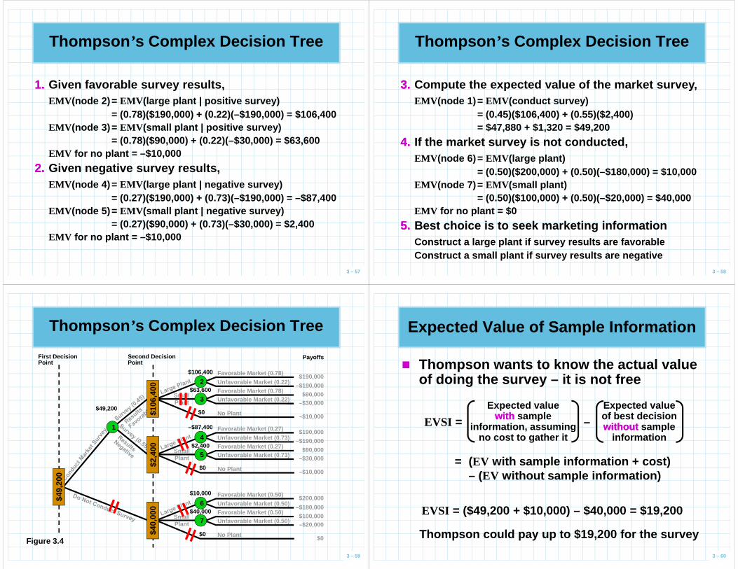
Thompson ’s Complex Decision Tree
1.1. Given favorable survey results,EMV (node 2)= EMV (large plant | positive survey)
= (0.78)($190,000) + (0.22)(–$190,000) = $106,400EMV (node 3)= EMV (small plant | positive survey)
= (0.78)($90,000) + (0.22)(–$30,000) = $63,600
3 – 57
= (0.78)($90,000) + (0.22)(–$30,000) = $63,600EMV for no plant = –$10,000
2.2. Given negative survey results,EMV (node 4)= EMV (large plant | negative survey)
= (0.27)($190,000) + (0.73)(–$190,000) = –$87,400EMV (node 5)= EMV (small plant | negative survey)
= (0.27)($90,000) + (0.73)(–$30,000) = $2,400EMV for no plant = –$10,000
Thompson ’s Complex Decision Tree
3.3. Compute the expected value of the market survey,EMV (node 1)= EMV (conduct survey)
= (0.45)($106,400) + (0.55)($2,400)= $47,880 + $1,320 = $49,200
4.4. If the market survey is not conducted,
3 – 58
4.4. If the market survey is not conducted,EMV (node 6)= EMV (large plant)
= (0.50)($200,000) + (0.50)(–$180,000) = $10,000EMV (node 7)= EMV (small plant)
= (0.50)($100,000) + (0.50)(–$20,000) = $40,000EMV for no plant = $0
5.5. Best choice is to seek marketing informationConstruct a large plant if survey results are favor ableConstruct a small plant if survey results are negat ive
Thompson ’s Complex Decision Tree
First Decision Point
Second Decision Point
Favorable Market (0.78)
Unfavorable Market (0.22)Favorable Market (0.78)Unfavorable Market (0.22)
Favorable Market (0.27)
Small Plant
No Plant
2
3
1
Payoffs
–$190,000
$190,000
$90,000–$30,000
–$10,000$106
,400
$106,400
$63,600
–$87,400
$49,200$0
3 – 59
Figure 3.4
Favorable Market (0.27)
Unfavorable Market (0.73)Favorable Market (0.27)Unfavorable Market (0.73)
Favorable Market (0.50)
Unfavorable Market (0.50)Favorable Market (0.50)Unfavorable Market (0.50)
Small Plant
No Plant
6
7
Small Plant
No Plant
4
5
1
–$180,000
$200,000
$100,000–$20,000
$0
–$190,000
$190,000
$90,000–$30,000
–$10,000
$40,
000
$2,4
00
$49,
200
–$87,400
$2,400
$10,000
$40,000
$0
$0
Expected Value of Sample Information
� Thompson wants to know the actual value of doing the survey – it is not free
EVSI = –Expected value
withwith sampleinformation, assuming
Expected valueof best decisionwithoutwithout sample
3 – 60
EVSI = –information, assumingno cost to gather it
withoutwithout sampleinformation
= (EV with sample information + cost)– (EV without sample information)
EVSI = ($49,200 + $10,000) – $40,000 = $19,200
Thompson could pay up to $19,200 for the survey
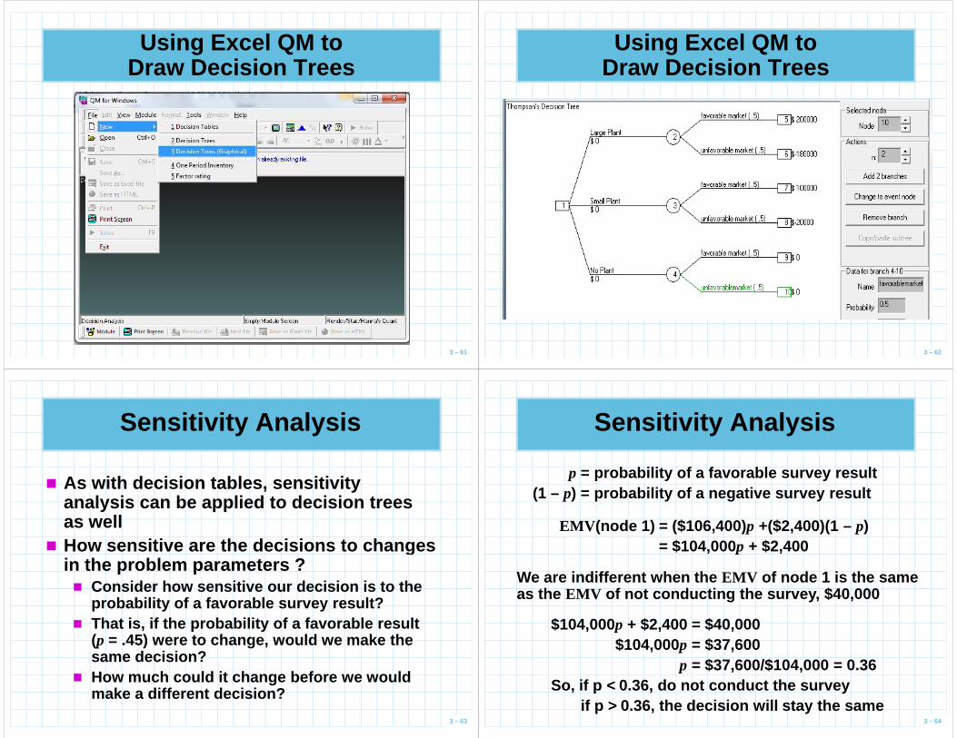
Using Excel QM to Draw Decision Trees
3 – 61
Using Excel QM to Draw Decision Trees
3 – 62
Sensitivity Analysis
� As with decision tables, sensitivity analysis can be applied to decision trees as well
� How sensitive are the decisions to changes
3 – 63
� How sensitive are the decisions to changes in the problem parameters ?� Consider how sensitive our decision is to the
probability of a favorable survey result? � That is, if the probability of a favorable result
(p = .45) were to change, would we make the same decision?
� How much could it change before we would make a different decision?
Sensitivity Analysis
p = probability of a favorable survey result(1 – p) = probability of a negative survey result
EMV (node 1) = ($106,400) p +($2,400)(1 – p)= $104,000p + $2,400
3 – 64
= $104,000p + $2,400
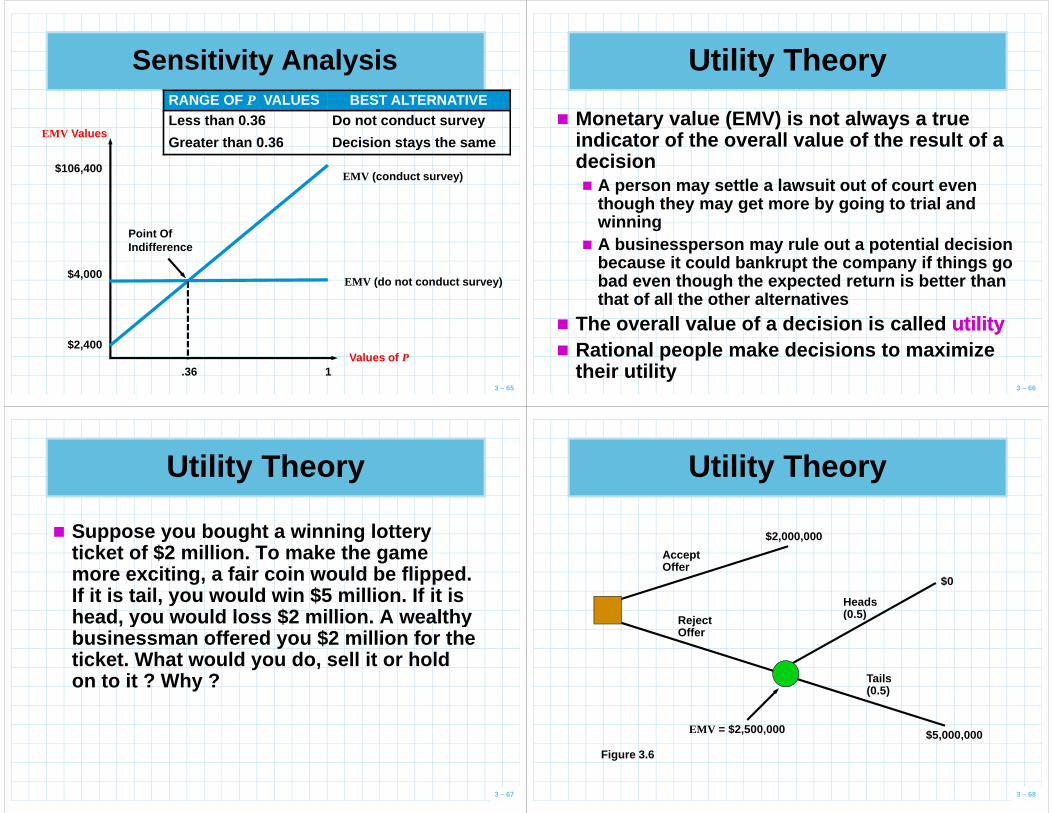
We are indifferent when the EMV of node 1 is the same as the EMV of not conducting the survey, $40,000
$104,000p + $2,400 = $40,000$104,000p = $37,600
p = $37,600/$104,000 = 0.36So, if p <<<< 0.36, do not conduct the survey
if p >>>> 0.36, the decision will stay the same
Sensitivity Analysis
$106,400
EMV Values
EMV (conduct survey)
RANGE OF P VALUES BEST ALTERNATIVELess than 0.36 Do not conduct survey
Greater than 0.36 Decision stays the same
3 – 65
$4,000
$2,400
EMV (do not conduct survey)
Point Of Indifference
.36 1Values of P
Utility Theory
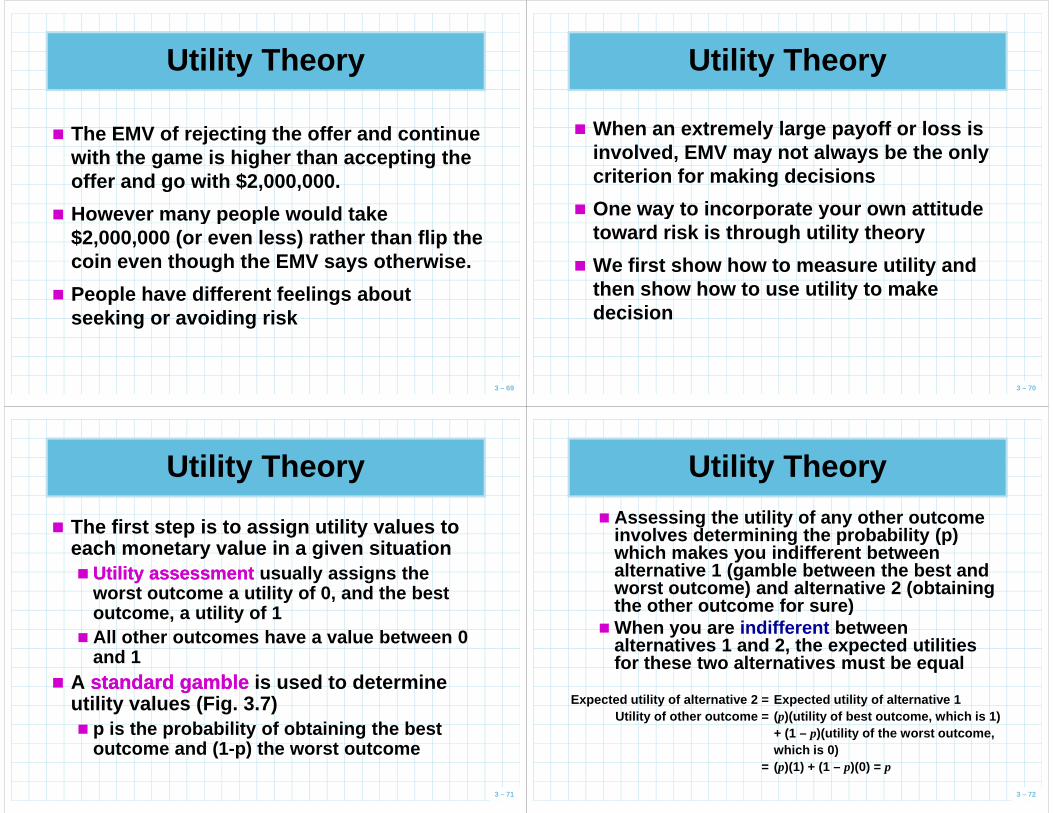
� Monetary value (EMV) is not always a true indicator of the overall value of the result of a decision� A person may settle a lawsuit out of court even
though they may get more by going to trial and
3 – 66
though they may get more by going to trial and winning
� A businessperson may rule out a potential decision because it could bankrupt the company if things go bad even though the expected return is better than that of all the other alternatives
� The overall value of a decision is called utilityutility� Rational people make decisions to maximize
their utility
Utility Theory
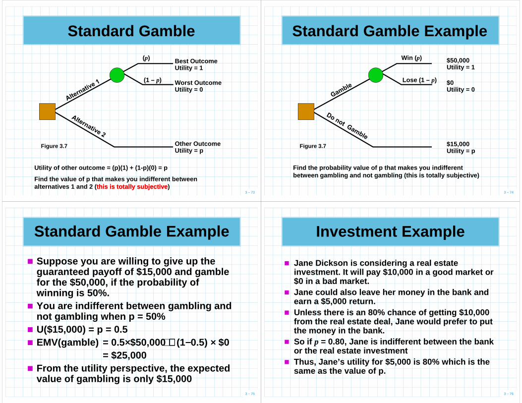
� Suppose you bought a winning lottery ticket of $2 million. To make the game more exciting, a fair coin would be flipped. If it is tail, you would win $5 million. If it is head, you would loss $2 million. A wealthy
3 – 67
head, you would loss $2 million. A wealthy businessman offered you $2 million for the ticket. What would you do, sell it or hold on to it ? Why ?
Heads (0.5)
$0
Utility Theory
Accept Offer
$2,000,000
3 – 68
(0.5)
Tails (0.5)
$5,000,000
Reject Offer
EMV = $2,500,000
Figure 3.6
Utility Theory
� The EMV of rejecting the offer and continue with the game is higher than accepting the offer and go with $2,000,000.
However many people would take
3 – 69
� However many people would take $2,000,000 (or even less) rather than flip the coin even though the EMV says otherwise.
� People have different feelings about seeking or avoiding risk
Utility Theory
� When an extremely large payoff or loss is involved, EMV may not always be the only criterion for making decisions
� One way to incorporate your own attitude
3 – 70
� One way to incorporate your own attitude toward risk is through utility theory
� We first show how to measure utility and then show how to use utility to make decision
Utility Theory
� The first step is to assign utility values to each monetary value in a given situation�� Utility assessmentUtility assessment usually assigns the
worst outcome a utility of 0, and the best outcome, a utility of 1
3 – 71
outcome, a utility of 1� All other outcomes have a value between 0
and 1� A standard gamblestandard gamble is used to determine
utility values (Fig. 3.7)� p is the probability of obtaining the best
outcome and (1- p) the worst outcome
Utility Theory
� Assessing the utility of any other outcome involves determining the probability ( p) which makes you indifferent between alternative 1 (gamble between the best and worst outcome) and alternative 2 (obtaining the other outcome for sure)
3 – 72
the other outcome for sure)� When you are indifferent between
alternatives 1 and 2, the expected utilities for these two alternatives must be equal
Expected utility of alternative 2 = Expected utility of alternative 1Utility of other outcome = ( p)(utility of best outcome, which is 1)
+ (1 – p)(utility of the worst outcome, which is 0)
= (p)(1) + (1 – p)(0) = p
Standard Gamble
Best OutcomeUtility = 1
Worst OutcomeUtility = 0
(p)
(1 – p)
3 – 73
Other OutcomeUtility = p
Figure 3.7
Utility of other outcome = (p)(1) + (1-p)(0) = p
Find the value of p that makes you indifferent betw een alternatives 1 and 2 ( this is totally subjectivethis is totally subjective )
Standard Gamble Example
$50,000Utility = 1
$0Utility = 0
Win (p)
Lose (1 – p)
3 – 74
$15,000Utility = p
Figure 3.7
Find the probability value of p that makes you indi fferent between gambling and not gambling (this is totally subjective)
� Suppose you are willing to give up the guaranteed payoff of $15,000 and gamble for the $50,000, if the probability of winning is 50%.
� You are indifferent between gambling and
Standard Gamble Example
3 – 75
� You are indifferent between gambling and not gambling when p = 50%
� U($15,000) = p = 0.5� EMV(gamble) = 0.5 ××××$50,000 ++++ (1−−−−0.5) ×××× $0
= $25,000� From the utility perspective, the expected
value of gambling is only $15,000
Investment Example
� Jane Dickson is considering a real estate investment. It will pay $10,000 in a good market or $0 in a bad market.
� Jane could also leave her money in the bank and earn a $5,000 return.
3 – 76
earn a $5,000 return. � Unless there is an 80% chance of getting $10,000
from the real estate deal, Jane would prefer to put the money in the bank.
� So if p = 0.80, Jane is indifferent between the bank or the real estate investment
� Thus, Jane’s utility for $5,000 is 80% which is the same as the value of p.
Investment Example
p = 0.80
(1 – p) = 0.20
$10,000U($10,000) = 1.0
$0U($0.00) = 0.0
3 – 77
Figure 3.8
$5,000U($5,000) = p = 0.8
Utility for $5,000 = U($5,000) = p = 0.8
Investment Example
Utility for $7,000 = 0.90Utility for $3,000 = 0.50
� We can assess other utility values in the same way� For Jane these are
3 – 78
Utility for $3,000 = 0.50
� Jane Dickson wants to construct a utility curve revealing her preference for money between $0 and $10,000 under the risk
� A utility curve plots the utility value versus the monetary value
� Using the three utilities for different dollar amou nts, it is enough to construct a utility curve assessing Jane’s feeling toward risk
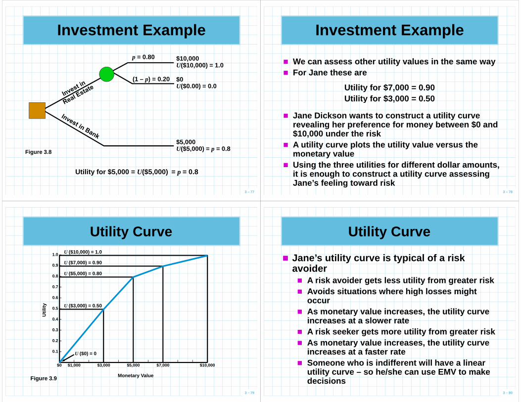
Utility Curve
U ($7,000) = 0.90
U ($5,000) = 0.80
1.0 –
0.9 –
0.8 –
0.7 –
0.6 –
U ($10,000) = 1.0
3 – 79
U ($3,000) = 0.50
U ($0) = 0
Figure 3.9
0.5 –
0.4 –
0.3 –
0.2 –
0.1 –
| | | | | | | | | | |
$0 $1,000 $3,000 $5,000 $7,000 $10,000
Monetary Value
Util
ity
Utility Curve
� Jane’s utility curve is typical of a risk avoider� A risk avoider gets less utility from greater risk� Avoids situations where high losses might
occur
3 – 80
occur� As monetary value increases, the utility curve
increases at a slower rate� A risk seeker gets more utility from greater risk� As monetary value increases, the utility curve
increases at a faster rate� Someone who is indifferent will have a linear
utility curve – so he/she can use EMV to make decisions
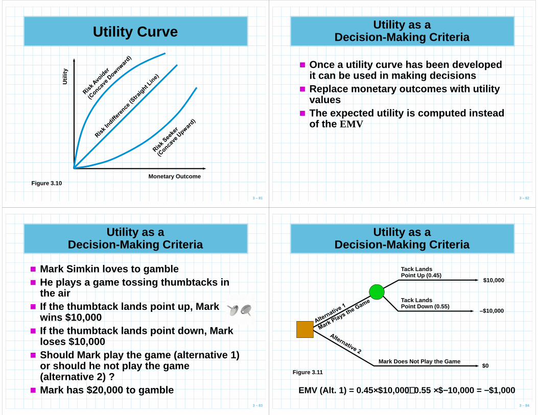
Utility Curve
Util
ity
3 – 81
Figure 3.10Monetary Outcome
Utility as a Decision-Making Criteria
� Once a utility curve has been developed it can be used in making decisions
� Replace monetary outcomes with utility values
3 – 82
values� The expected utility is computed instead
of the EMV
Utility as a Decision-Making Criteria
� Mark Simkin loves to gamble� He plays a game tossing thumbtacks in
the air� If the thumbtack lands point up, Mark
3 – 83
� If the thumbtack lands point up, Mark wins $10,000
� If the thumbtack lands point down, Mark loses $10,000
� Should Mark play the game (alternative 1) or should he not play the game (alternative 2) ?
� Mark has $20,000 to gamble
Utility as a Decision-Making Criteria
Tack Lands Point Up (0.45)
$10,000
–$10,000
Tack Lands Point Down (0.55)
3 – 84
Figure 3.11
–$10,000
$0Mark Does Not Play the Game
EMV (Alt. 1) = 0.45 ××××$10,000++++0.55 ××××$−−−−10,000 = −−−−$1,000
Utility as a Decision-Making Criteria
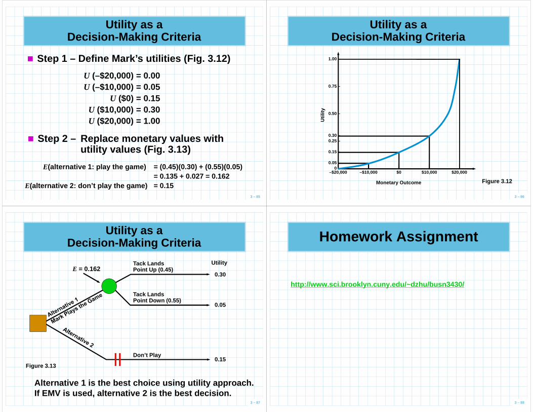
� Step 1 – Define Mark’s utilities (Fig. 3.12)
U (–$20,000) = 0.00U (–$10,000) = 0.05
U ($0) = 0.15
3 – 85
U ($10,000) = 0.30U ($20,000) = 1.00
� Step 2 – Replace monetary values withutility values (Fig. 3.13)
E(alternative 1: play the game) = (0.45)(0.30) + (0.5 5)(0.05)= 0.135 + 0.027 = 0.162
E(alternative 2: don’t play the game) = 0.15
Utility as a Decision-Making Criteria
1.00 –
0.75 –
3 – 86
Figure 3.12
0.50 –
0.30 –0.25 –
0.15 –
0.05 –0 –| | | | |
–$20,000 –$10,000 $0 $10,000 $20,000
Monetary Outcome
Util
ity
Utility as a Decision-Making Criteria
Tack Lands Point Up (0.45)
0.30
0.05
Tack Lands Point Down (0.55)
UtilityE = 0.162
3 – 87
Figure 3.130.15
Don’t Play
Alternative 1 is the best choice using utility appr oach.If EMV is used, alternative 2 is the best decision.
http://www.sci.brooklyn.cuny.edu/~dzhu/busn3430/
Homework Assignment
3 – 88