Embed Size (px)
Citation preview
1
DECISION ANALYSIS
Introduction
Decision often must be made in uncertainenvironments.Examples:
Manufacturer introducing a new product in themarketplace.Government contractor bidding on a new contract.Oil company deciding to drill for oil in a particularlocation.
Type of decisions that decision analysis is designed toaddress.Making decisions with or without experimentation.
558
2
Prototype example
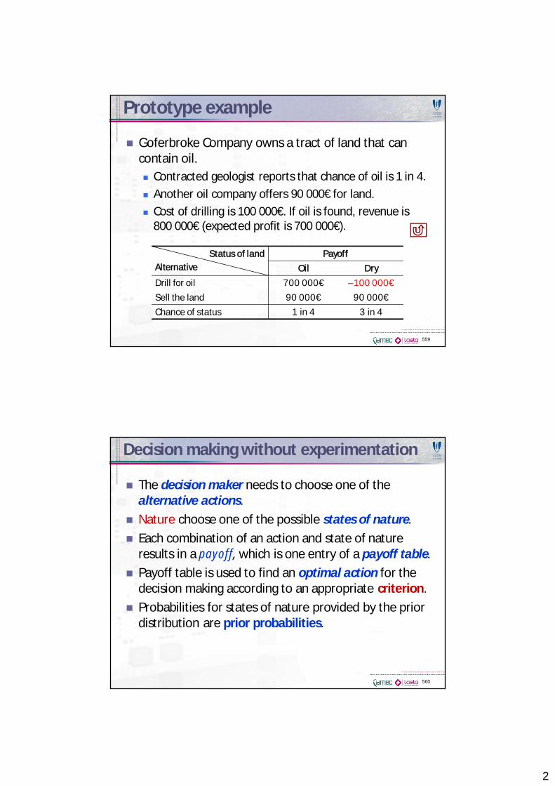
Goferbroke Company owns a tract of land that cancontain oil.
Contracted geologist reports that chance of oil is 1 in 4.Another oil company offers 90 000€ for land.Cost of drilling is 100 000€. If oil is found, revenue is800 000€ (expected profit is 700 000€).
559
Status of landAlternative
PayoffOil Dry
Drill for oil 700 000€ –100 000€Sell the land 90 000€ 90 000€Chance of status 1 in 4 3 in 4
Decision making without experimentation
The decision maker needs to choose one of thealternative actions.Nature choose one of the possible states of nature.Each combination of an action and state of natureresults in a payoff, which is one entry of a payoff table.Payoff table is used to find an optimal action for thedecision making according to an appropriate criterion.Probabilities for states of nature provided by the priordistribution are prior probabilities.
560
3
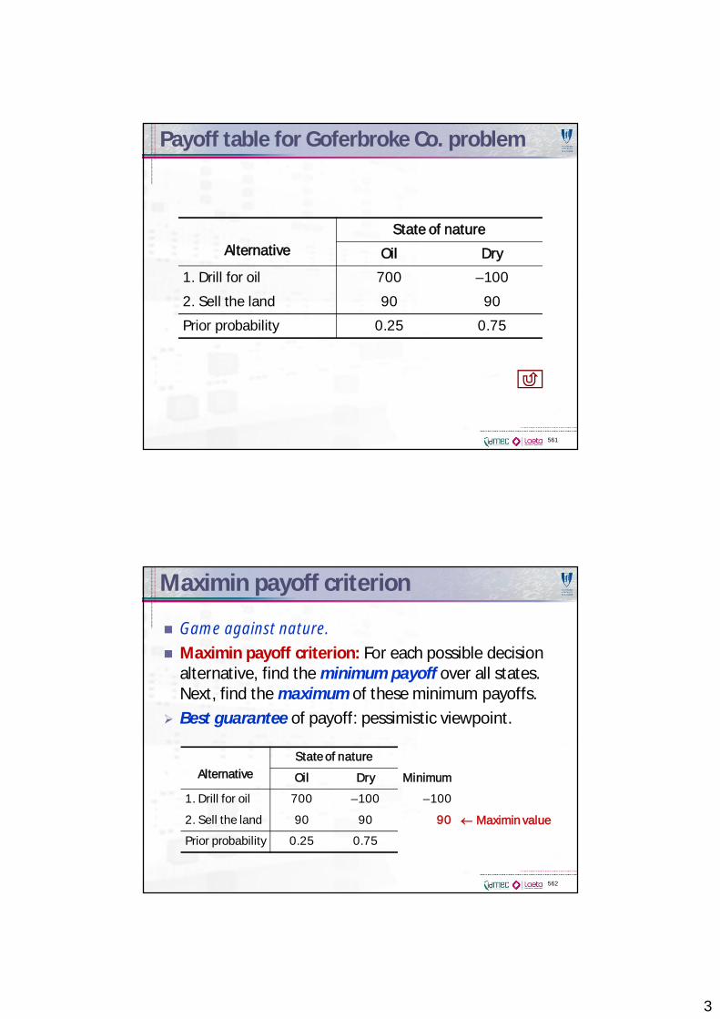
Payoff table for Goferbroke Co. problem
561
AlternativeState of nature
Oil Dry
1. Drill for oil 700 –100
2. Sell the land 90 90
Prior probability 0.25 0.75
Maximin payoff criterion
Game against nature.Maximin payoff criterion: For each possible decisionalternative, find the minimum payoff over all states.Next, find the maximum of these minimum payoffs.Best guarantee of payoff: pessimistic viewpoint.
562
AlternativeState of nature
Oil Dry Minimum
1. Drill for oil 700 –100 –100
2. Sell the land 90 90 90 Maximin value
Prior probability 0.25 0.75
4
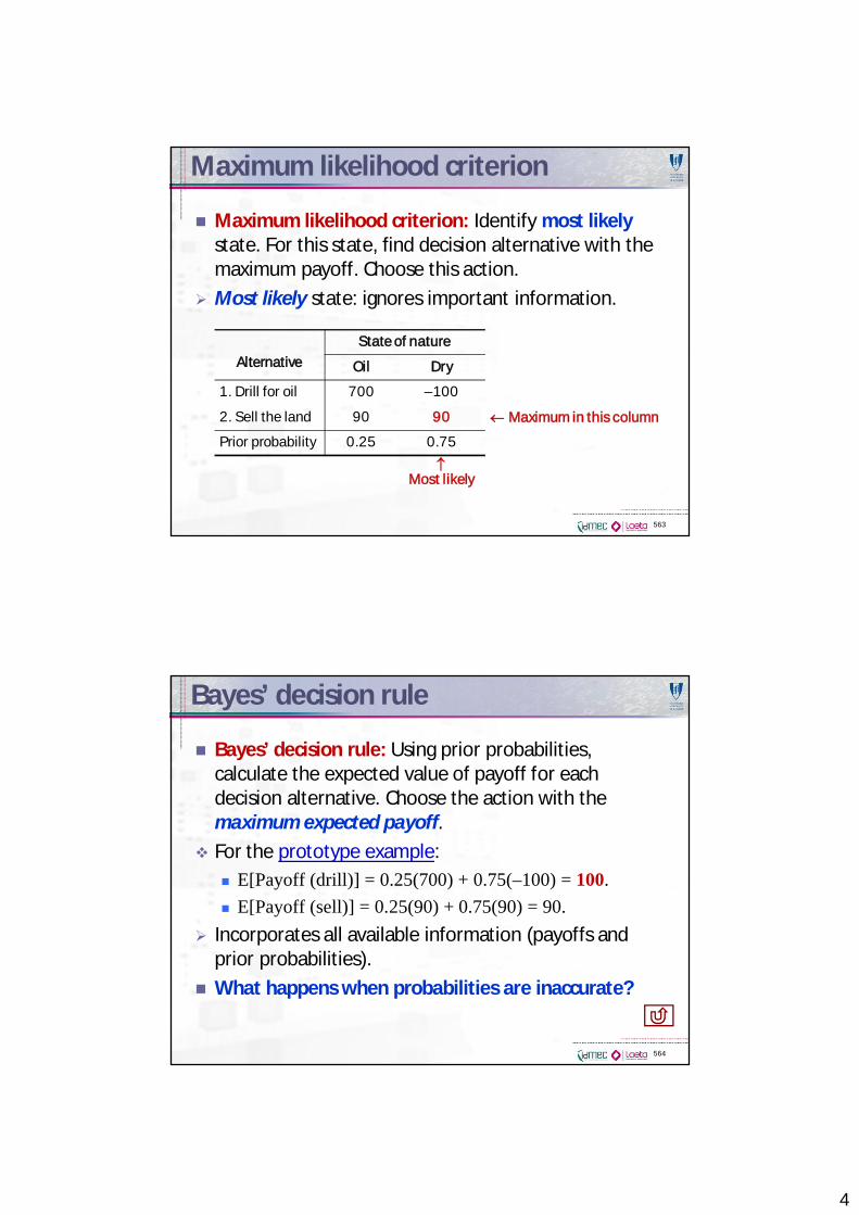
Maximum likelihood criterion
Maximum likelihood criterion: Identify most likelystate. For this state, find decision alternative with themaximum payoff. Choose this action.Most likely state: ignores important information.
563
AlternativeState of nature
Oil Dry
1. Drill for oil 700 –100
2. Sell the land 90 90 Maximum in this column
Prior probability 0.25 0.75
Most likely
Bayes’ decision rule
Bayes’ decision rule: Using prior probabilities,calculate the expected value of payoff for eachdecision alternative. Choose the action with themaximum expected payoff.For the prototype example:
E[Payoff (drill)] = 0.25(700) + 0.75(–100) = 100.E[Payoff (sell)] = 0.25(90) + 0.75(90) = 90.
Incorporates all available information (payoffs andprior probabilities).What happens when probabilities are inaccurate?
564
5
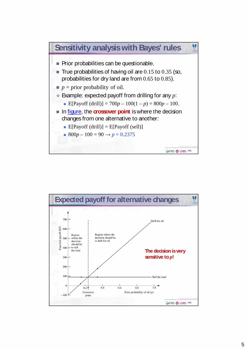
Sensitivity analysis with Bayes’ rules
Prior probabilities can be questionable.True probabilities of having oil are 0.15 to 0.35 (so,probabilities for dry land are from 0.65 to 0.85).p = prior probability of oil.Example: expected payoff from drilling for any p:
E[Payoff (drill)] = 700p – 100(1 – p) = 800p – 100.In figure, the crossover point is where the decisionchanges from one alternative to another:
E[Payoff (drill)] = E[Payoff (sell)]800p – 100 = 90 p = 0.2375
565
Expected payoff for alternative changes
566
The decision is verysensitive to p!
6
Decision making with experimentation
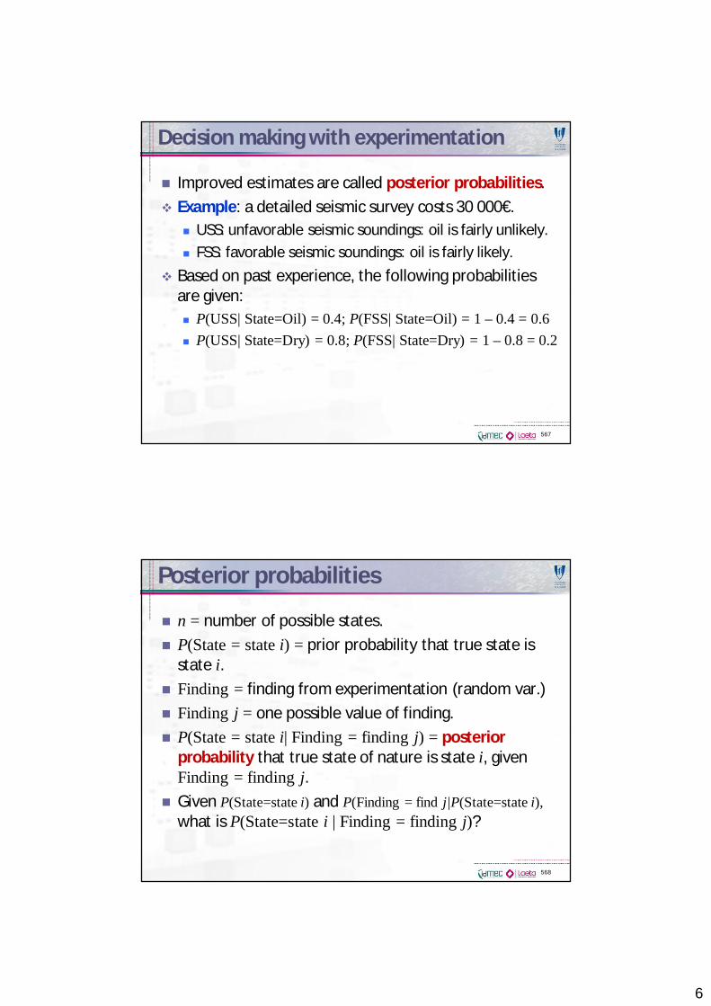
Improved estimates are called posterior probabilities.Example: a detailed seismic survey costs 30 000€.
USS: unfavorable seismic soundings: oil is fairly unlikely.FSS: favorable seismic soundings: oil is fairly likely.
Based on past experience, the following probabilitiesare given:
P(USS| State=Oil) = 0.4; P(FSS| State=Oil) = 1 – 0.4 = 0.6P(USS| State=Dry) = 0.8; P(FSS| State=Dry) = 1 – 0.8 = 0.2
567
Posterior probabilities
n = number of possible states.P(State = state i) = prior probability that true state isstate i.Finding = finding from experimentation (random var.)Finding j = one possible value of finding.P(State = state i| Finding = finding j) = posteriorprobability that true state of nature is state i, givenFinding = finding j.Given P(State=state i) and P(Finding = find j|P(State=state i),what is P(State=state i | Finding = finding j)?
568
7
Posterior probabilities
From probability theory the Bayes’ theorem can beobtained:
569
1
(State = state | Finding = finding )
(Finding = finding |State = state ) (State = state )
(Finding = finding |State = state ) (State = state )n
k
P i j
P j i P i
P j k P k
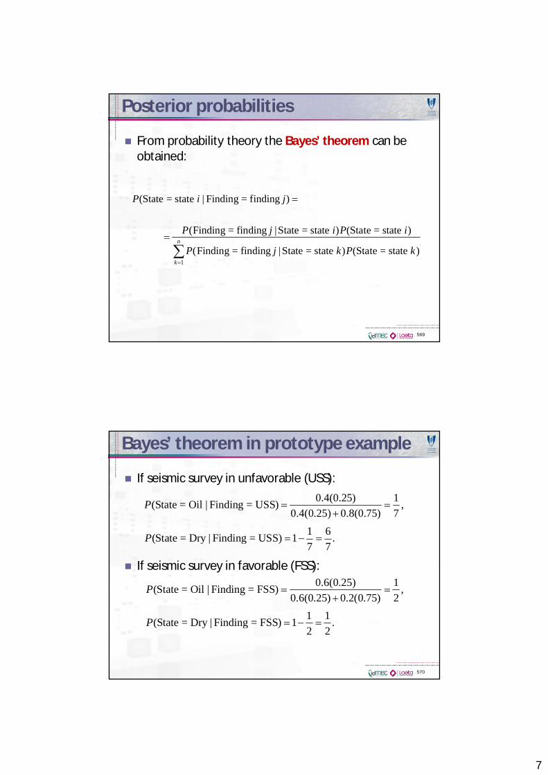
Bayes’ theorem in prototype example
If seismic survey in unfavorable (USS):
If seismic survey in favorable (FSS):
570
0.4(0.25) 1(State = Oil | Finding = USS) ,0.4(0.25) 0.8(0.75) 7
P
1 6(State = Dry | Finding = USS) 1 .7 7
P
0.6(0.25) 1(State = Oil | Finding = FSS) ,0.6(0.25) 0.2(0.75) 2
P
1 1(State = Dry | Finding = FSS) 1 .2 2
P
8
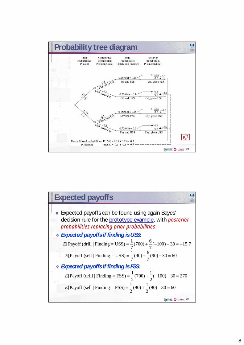
Probability tree diagram
571
Expected payoffs
Expected payoffs can be found using again Bayes’decision rule for the prototype example, with posteriorprobabilities replacing prior probabilities:Expected payoffs if finding is USS:
Expected payoffs if finding is FSS:
572
1 6[Payoff (drill | Finding = USS) (700) ( 100) 30 15.77 7
E
1 6[Payoff (sell | Finding = USS) (90) (90) 30 607 7
E
1 1[Payoff (drill | Finding = FSS) (700) ( 100) 30 2702 2
E
1 1[Payoff (sell | Finding = FSS) (90) (90) 30 602 2
E
9
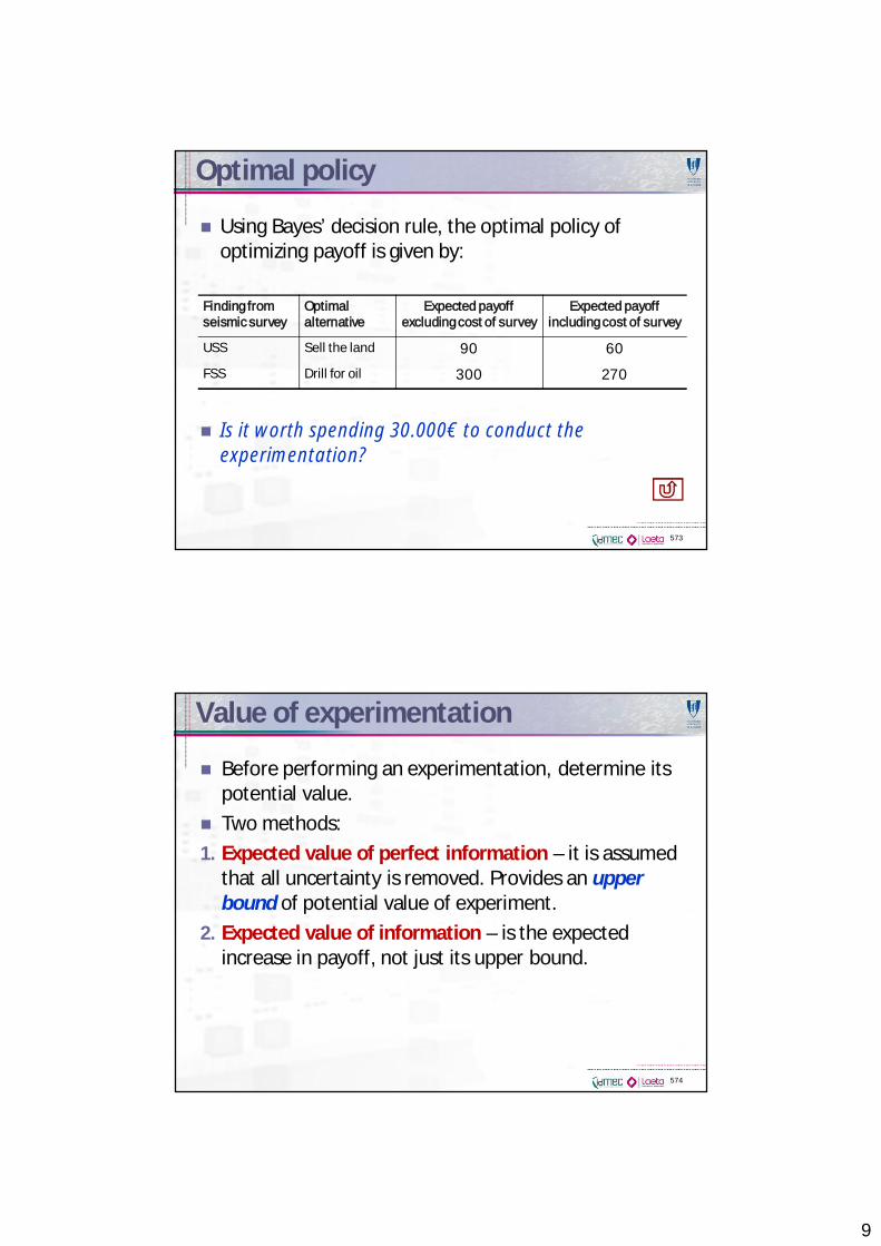
Optimal policy
Using Bayes’ decision rule, the optimal policy ofoptimizing payoff is given by:
Is it worth spending 30.000€ to conduct theexperimentation?
573
Finding fromseismic survey
Optimalalternative
Expected payoffexcluding cost of survey
Expected payoffincluding cost of survey
USS Sell the land 90 60
FSS Drill for oil 300 270
Value of experimentation
Before performing an experimentation, determine itspotential value.Two methods:
1. Expected value of perfect information – it is assumedthat all uncertainty is removed. Provides an upperbound of potential value of experiment.
2. Expected value of information – is the expectedincrease in payoff, not just its upper bound.
574
10
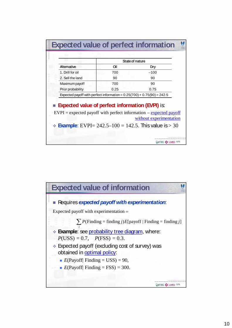
Expected value of perfect information
Expected value of perfect information (EVPI) is:EVPI = expected payoff with perfect information – expected payoff
without experimentationExample: EVPI= 242.5–100 = 142.5. This value is > 30
575
State of natureAlternative Oil Dry1. Drill for oil 700 –1002. Sell the land 90 90Maximum payoff 700 90Prior probability 0.25 0.75Expected payoff with perfect information = 0.25(700) + 0.75(90) = 242.5
Expected value of information
Requires expected payoff with experimentation:
Example: see probability tree diagram, where:P(USS) = 0.7, P(FSS) = 0.3.Expected payoff (excluding cost of survey) wasobtained in optimal policy:
E(Payoff| Finding = USS) = 90,E(Payoff| Finding = FSS) = 300.
576
Expected payoff with experimentation
(Finding = finding ) [payoff | Finding = finding ]j
P j E j
11
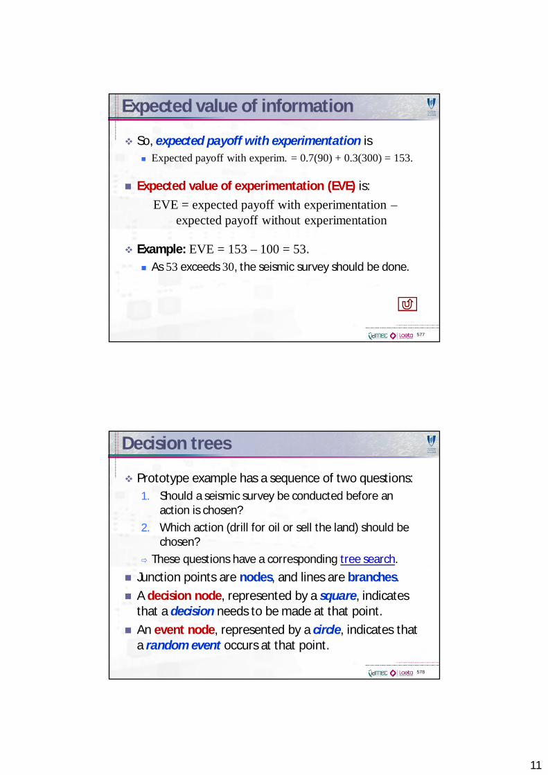
Expected value of information
So, expected payoff with experimentation isExpected payoff with experim. = 0.7(90) + 0.3(300) = 153.
Expected value of experimentation (EVE) is:EVE = expected payoff with experimentation –
expected payoff without experimentation
Example: EVE = 153 – 100 = 53.As 53 exceeds 30, the seismic survey should be done.
577
Decision trees
Prototype example has a sequence of two questions:1. Should a seismic survey be conducted before an
action is chosen?2. Which action (drill for oil or sell the land) should be
chosen?These questions have a corresponding tree search.
Junction points are nodes, and lines are branches.A decision node, represented by a square, indicatesthat a decision needs to be made at that point.An event node, represented by a circle, indicates thata random event occurs at that point.
578
12
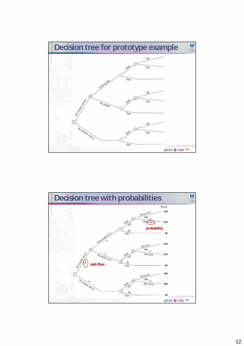
Decision tree for prototype example
579
Decision tree with probabilities
580
cash flow
probability
13
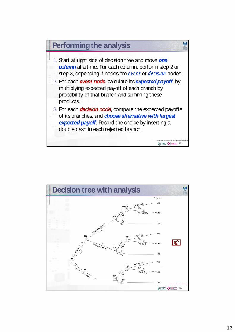
Performing the analysis
1. Start at right side of decision tree and move onecolumn at a time. For each column, perform step 2 orstep 3, depending if nodes are event or decision nodes.
2. For each event node, calculate its expected payoff, bymultiplying expected payoff of each branch byprobability of that branch and summing theseproducts.
3. For each decision node, compare the expected payoffsof its branches, and choose alternative with largestexpected payoff. Record the choice by inserting adouble dash in each rejected branch.
581
Decision tree with analysis
582
14
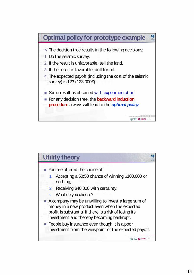
Optimal policy for prototype example
The decision tree results in the following decisions:1. Do the seismic survey.2. If the result is unfavorable, sell the land.3. If the result is favorable, drill for oil.4. The expected payoff (including the cost of the seismic
survey) is 123 (123 000€).
Same result as obtained with experimentation.For any decision tree, the backward inductionprocedure always will lead to the optimal policy.
583
Utility theory
You are offered the choice of:1. Accepting a 50:50 chance of winning $100.000 or
nothing;2. Receiving $40.000 with certainty.
What do you choose?A company may be unwilling to invest a large sum ofmoney in a new product even when the expectedprofit is substantial if there is a risk of losing itsinvestment and thereby becoming bankrupt.People buy insurance even though it is a poorinvestment from the viewpoint of the expected payoff.
584
15
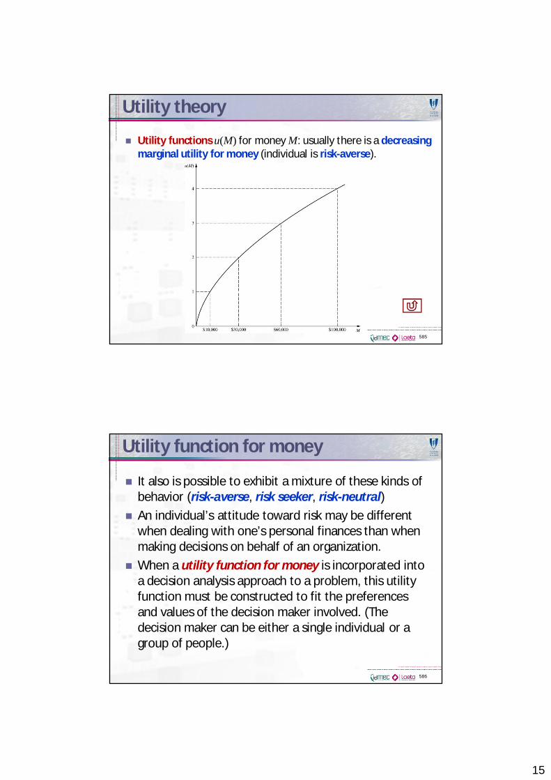
Utility theory
Utility functions u(M) for money M: usually there is a decreasingmarginal utility for money (individual is risk-averse).
585
Utility function for money
It also is possible to exhibit a mixture of these kinds ofbehavior (risk-averse, risk seeker, risk-neutral)An individual’s attitude toward risk may be differentwhen dealing with one’s personal finances than whenmaking decisions on behalf of an organization.When a utility function for money is incorporated intoa decision analysis approach to a problem, this utilityfunction must be constructed to fit the preferencesand values of the decision maker involved. (Thedecision maker can be either a single individual or agroup of people.)
586
16
Utility theory
Fundamental property: the decision maker’s utilityfunction for money has the property that the decisionmaker is indifferent between two alternatives if theyhave the same expected utility.Example. Offer: an opportunity to obtain either$100000 (utility = 4) with probability p or nothing(utility = 0) with probability 1 – p. Thus, E(utility) = 4p.
Decision maker is indifferent for e.g.:Offer with p = 0.25 (E(utility) = 1) or definitelyobtaining $10 000 (utility = 1).Offer with p = 0.75 (E(utility) = 3) or definitelyobtaining $60 000 (utility = 3).
587
Role of utility theory
If utility function is used to measure worth of possiblemonetary outcomes, Bayes’ decision rule replacesmonetary payoffs by corresponding utilities.Thus, optimal action is the one that maximizes theexpected utility.
Note that utility functions my not be monetary.Example: doctor’s decision alternatives in treating apatient involves the future health of the patient.
588
17
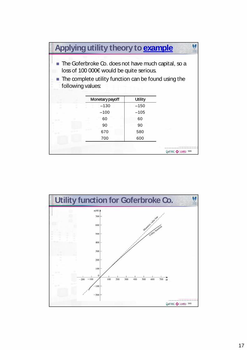
Applying utility theory to example
The Goferbroke Co. does not have much capital, so aloss of 100 000€ would be quite serious.The complete utility function can be found using thefollowing values:
589
Monetary payoff Utility–130 –150–100 –105
60 6090 90
670 580700 600
Utility function for Goferbroke Co.
590
18
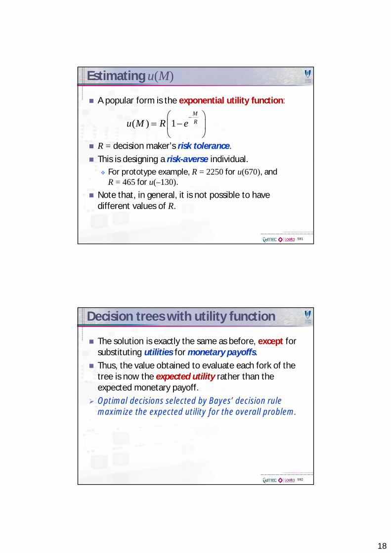
Estimating u(M)
A popular form is the exponential utility function:
R = decision maker’s risk tolerance.This is designing a risk-averse individual.
For prototype example, R = 2250 for u(670), andR = 465 for u(–130).
Note that, in general, it is not possible to havedifferent values of R.
591
( ) 1MRu M R e
Decision trees with utility function
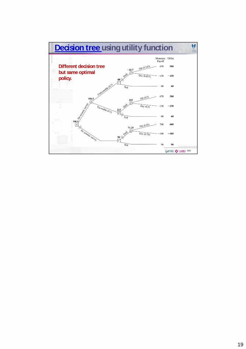
The solution is exactly the same as before, except forsubstituting utilities for monetary payoffs.Thus, the value obtained to evaluate each fork of thetree is now the expected utility rather than theexpected monetary payoff.Optimal decisions selected by Bayes’ decision rulemaximize the expected utility for the overall problem.
592
19
Decision tree using utility function
593
Different decision treebut same optimalpolicy.