Embed Size (px)
Citation preview

DECISION SUPPORT ANALYSIS FOR A RENEWABLE ENERGY SYSTEM TO SUPPLY A GRID-CONNECTED COMMERCIAL BUILDING
Andrew Tubesing Master of Science, Electrical Engineering
New Mexico Institute of Mining and Technology December 2009

© 2009 Andrew Tubesing All Rights Reserved

ABSTRACT
This thesis studies the integration of a solar concentrator photovoltaic array
(CPV) system with a commercial building. Solar resource conversion, load
characterization, power quality, and grid integration are the primary aspects addressed by
the study. Local solar radiation and renewable energy source (RES) conversion data were
used to determine a profile for annual energy production of the CPV, which uses a non-
traditional method of solar energy conversion. The load was characterized by creating an
annual profile for the building’s power demand using a combination of historical monthly
billing data and a week of detailed real-time power consumption data (real, reactive, and
apparent). Various simulation approaches were considered to evaluate the integration of
system components with the supply grid. Because of the high time resolution necessary
for the study, which evaluates a number of parameters that traditional methods do not
address, a custom analysis was performed, both in time segments and total project
lifetime figures. This quantifies, at one-minute resolution, the energy produced by the
RES, consumed by the building, and metered to and from the supply grid.
The study concludes that the CPV system will make a valuable contribution to the
energy supply, it can pay for itself in energy savings over a number of years, and it
provides a substantial environmental benefit by reducing pollutant emissions. Financial
considerations are dependent upon a number of variables, including the panel quantity,
buy/sell prices of grid energy, project lifetime, financing options, and renewable energy
credit programs.

ACKNOWLEDGMENTS
I would like to thank the numerous people who helped to make this project
possible.
At New Mexico Tech I would like to thank my research advisor and graduate
committee chair, Dr. Kevin Wedeward, whose interest and expertise allowed me to
explore this topic and provided valuable insight and assistance throughout the process.
Graduate committee members, Dr. Aly El-Osery and Dr. Bill Rison, provided much
appreciated help and guidance. Also I acknowledge Electrical Engineering department
chair, Dr. Scott Teare, whose support was instrumental in making the pursuit of this
degree possible.
From the Institute for Engineering Research and Applications (IERA) I wish to
thank Wes Helgeson. As a member of the Playas energy research project studied in this
thesis, he provided the impetus for this study as well as much supporting data on the site
and hardware.
I also owe a debt of gratitude to broadcast engineer Tom Nelson who gave me my
first job in electronics many years ago… a job which I desperately wanted, and it
profoundly shaped my future.
Thank you to all.
iii

TABLE OF CONTENTS
Title Page
ABSTRACT........................................................................................................................ ii ACKNOWLEDGMENTS ................................................................................................. iii TABLE OF CONTENTS................................................................................................... iv LIST OF FIGURES .............................................................................................................v LIST OF ACRONYMS AND ABBREVIATIONS ......................................................... vii Chapter 1 Introduction .........................................................................................................1 Chapter 2 Background .........................................................................................................6
2.1 Literature Review.................................................................................................... 6 2.2 Technical Concerns................................................................................................. 9
2.2.1 Power Balance ............................................................................................... 9 2.2.2 Time Dynamics & Transients ...................................................................... 10 2.2.3 Power Quality .............................................................................................. 12
Chapter 3 Methodology .....................................................................................................18 3.1 Physical System .................................................................................................... 18
3.1.1 Description................................................................................................... 18 3.1.2 Operational Modes....................................................................................... 20
3.2 Load Characterization........................................................................................... 21 3.2.1 Historical and Time Series Data .................................................................. 21 3.2.2 Seasonal and Annual Variation.................................................................... 27 3.2.3 Projected Annual Load Profile..................................................................... 29
3.3 Source Characterization ........................................................................................ 30 3.3.1 Solar Radiation and the CPV System .......................................................... 30 3.3.2 CPV Characterization .................................................................................. 32 3.3.3 Solar Irradiation Profile for the Installation Site.......................................... 38 3.3.4 Projected Annual Solar Source Profile ........................................................ 41
3.4 Analysis................................................................................................................. 42 3.4.1 Overview...................................................................................................... 42 3.4.2 Tools ............................................................................................................ 43 3.4.3 Computation................................................................................................. 45 3.4.4 Actual vs. Predicted Value Check ............................................................... 48 3.4.5 Results Interface........................................................................................... 51
3.5 System Characterization and Output Evaluation .................................................. 58 Chapter 4 Conclusion.........................................................................................................68 APPENDIX........................................................................................................................72 REFERENCES ..................................................................................................................76
iv

LIST OF FIGURES
Figure Page
Figure 1: Power triangle for positive power factor angle ................................................. 15
Figure 2: Monthly energy consumption based on utility meter readings ......................... 22
Figure 3: Weekly profile of real power, per phase ........................................................... 23
Figure 4: Weekly profile of reactive power, per phase..................................................... 23
Figure 5: Weekly profile of apparent power, per phase.................................................... 23
Figure 6: Weekly profile of power consumption from time series data ........................... 26
Figure 7: Monthly median temperatures at Hachita NM.................................................. 28
Figure 8: Emcore Concentrator Photovoltaic Array ......................................................... 32
Figure 9: Daily CPV output profile based on experimental data from 9/4/2008.............. 33
Figure 10: ISIS solar irradiation profile for Albuquerque NM on 9/4/2008..................... 33
Figure 11: Electric conversion profile for CPV panel ...................................................... 34
Figure 12: Electric conversion profile with polynomials ................................................. 36
Figure 13: Single day CPV power output: experimental and theoretical values .............. 37
Figure 14: Map of Playas NM region ............................................................................... 39
Figure 15: Expected CPV power output comparison ....................................................... 48
Figure 16: Load comparison: Actual vs. profile ............................................................... 49
Figure 17: Power balance for profiled data sets................................................................ 50
Figure 18: Power balance for actual data sets................................................................... 50
v
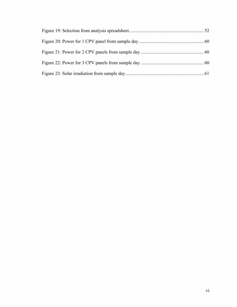
Figure 19: Selection from analysis spreadsheet................................................................ 52
Figure 20: Power for 1 CPV panel from sample day........................................................ 60
Figure 21: Power for 2 CPV panels from sample day ...................................................... 60
Figure 22: Power for 3 CPV panels from sample day ...................................................... 60
Figure 23: Solar irradiation from sample day ................................................................... 61
vi

LIST OF ACRONYMS AND ABBREVIATIONS
A Amperes (amps) RMS
AC Alternating Current
C&CC Command & Control Center
CPV Concentrator photovoltaic
CT Current transformer
DC Direct Current
DSS Decision Support System
kWH Kilowatt-hour
MWH Megawatt-hour (1000 kWH)
NOAA National Oceanic and Atmospheric Administration
P Real (active) power
PV Photovoltaic
Q Reactive power
RES ` Renewable energy source/s
REC Renewable energy credit/s
S Complex power (|S| = Apparent power)
θ Theta (power factor angle)
V Volts RMS
W Watts
vii

1
CHAPTER 1 INTRODUCTION
As renewable energy sources (RES) gain popularity throughout the world, it
becomes increasingly important to predict their value to a proposed electric power system
that would include them. This allows energy customers to evaluate the technical
feasibility, cost, benefit, and environmental factors in making a decision to integrate RES
into their power supply. As evidenced by the questions that led to this thesis project, and
the literature contributed by industry and academia on the topic, this is a valuable and
timely course of study [1,2,3,10,13]. Many projects around the world are venturing to
answer questions about how RES behave in hybrid systems and what the technical,
financial, and environmental implications are for their inclusion.
The town of Playas, New Mexico is an isolated community served by a single
electric utility feeder line from Columbus Electric Cooperative. This offers a unique
opportunity to study the benefit and impact of various approaches to electricity supply
and management of a microgrid and its components. Multiple projects are underway in
Playas that are intended to provide such insight. The project discussed in this thesis is one
such effort.
The system being studied in this case is a hybrid of renewable energy and grid
power. The facility managers intend to connect one or more solar Concentrator
Photovoltaic Array systems at or close to the utility feeder line into the town, and use it to
replace a portion of the grid power being used from the utility to feed the microgrid.

Since a comprehensive study of the microgrid itself has not been performed, its load
profile would be difficult to characterize with available data and is beyond the scope of
this study. However, there is an intermediate option. The largest single electricity
consumer in the microgrid is a commercial building, the Command and Control Center
(C&CC). Historical power usage data is available for all electric loads in the town, but
the C&CC is also being monitored in real time, in much greater detail. Real power,
reactive power, apparent power, voltage, current, power factor, and associated phase
angle are all being logged at one-minute intervals, providing time-series electricity usage
data. Additionally, there are separate monitors for each electrical sub-panel in the
building such that various categories of load types within the building can be
characterized separately.
This offers the opportunity to characterize the C&CC energy usage in much more
detail than any other component of the microgrid. Therefore, the project outlined here
will evaluate the interconnection of the solar array with the C&CC building. This will
generate a sample model for how the RES on site can be utilized by a load that is
characterized in one-minute resolution with enough detail to meaningfully evaluate the
short term characteristics. If or when such load characterization is available for the
remainder of the microgrid it could replace the C&CC profile in the analysis for a new
evaluation of the entire town.
The thesis work encompasses several stages. Starting with the Background
chapter, relevant scientific literature on the topic will be explored to illustrate the
relevance and industry context of the study. Additional background in the scientific
principles that govern the topics covered in this thesis are provided in that section.
2

Decision support tools will also be evaluated to make a final choice on the analysis
method.
The Methodology chapter covers a comprehensive description of the project’s
design, procedures, and analysis. This work is broken into five sections.
1. Description of the proposed system
2. Load characterization to determine the energy usage of the C&CC
3. Renewable energy source characterization to determine the energy resource on-site
and predict electricity generation using the desired solar CPV collection system
4. Grid integration analysis and system analysis using a combination of off-the-shelf and
custom-made computational tools
5. System characterization and feasibility analysis to determine the system’s energy use
impact, environmental impact, cost, and earning/savings potential
Stage 1 introduces the system and its composition. Stages 2 and 3 characterize the
physical components of the system. Stage 4 performs the analysis computations and
outputs the results. Stage 5 evaluates the financial and environmental factors to assist in
the overall system analysis.
Stage 2 investigates the energy usage of the C&CC building load. This is the load
characterization stage. It involves introductory work to gather data on the load
components and learn how and when they will operate in an effort to fully characterize
the power load and how it will change over time. This provides a theoretical description
of the power needs at the site that is based on historical data. Several years of monthly
3

power utility bills, along with one full week of power consumption measurements made
at one-minute resolution are be used to create the theoretical energy usage projections.
Stage 3 investigates the renewable energy conversion equipment and its
performance at the installation location. This is the source characterization stage. It
considers the use of one or more 25 kW concentrated photovoltaic solar array systems
manufactured by Emcore. System performance data and specifications, along with
meteorological data for the installation and test sites are combined to calculate the
expected energy harvested on-site.
Stage 4 addresses the decision support analysis used to characterize the load, grid
and RES interaction. It involves modeling of the system and simulation to determine how
the desired components will perform and interact with each other. Power factor analysis
of the load and source/s are performed to determine how to best characterize the load for
maximum accuracy in the simulation process and/or to determine the consumption
correction factor necessary in the case that the load is assumed to have an ideal power
factor of 1.0 in the analysis process. The necessity of transient analysis for load and
source power dynamics will be discussed as it relates to potential need for transient
suppression components. Finally, analysis tools are utilized to create a time series profile
of the interaction between load, RES, and grid energy. This provides a combined picture
of how much power will be needed from (and net metered back to) the utility’s electric
grid. The analysis will also provide financial projections for the system over the chosen
time span, and computation of pollutant emissions over that time. This information will
be used to characterize financial and environmental impacts and benefits of using RES
for this application.
4

Stage 5 evaluates the physical components against financial and environmental
factors to assist in the overall system analysis. It will consider the big picture perspective
of the previous three stages and make feasibility conclusions based on the results. This
portion will involve consideration of economics, environmental impact, and overall
energy usage of the building and its energy system.
Finally, the project is summarized in the Conclusion chapter where results and
implications are put into the context of their greater meaning. Future direction of this
work will also be discussed in the closing.
In a sense, this project is comprised of an effort to create a large amount of viable
data from a very small amount of information. It turns out that, with a few key sets of
experimental and historical data, the rest can be calculated, interpolated, and/or estimated
with acceptable accuracy. While attempting to minimize large assumptions and focus on
certainties that develop quality predictions, this project aims to provide decision analysis
of the proposed system that will be not only useful to the end user, but will do so with
reasonable certainty of the expected performance.
5

CHAPTER 2 BACKGROUND
2.1 Literature Review
As evidenced by the variety of research being conducted in the field, renewable
energy is a popular topic. Upon consideration of this project’s goals, a selection of
previous work in the field was investigated. Relevant literature falls into a number of
topic areas, including sustainable decision making in the energy context, decision support
systems (DSS), and technical resources.
Sustainable decision making is one of the clear motivators for the exploration of
renewable energy systems. Useful research on the topic goes back many years. An
exploration of this history was provided by Hersh [1]. This paper also introduces the
concept of the decision support systems and the role they play, both in the cultural
context and as a technical tool. Integrating renewable energy sources into the power
supply is a complex issue. There are social, environmental, financial, and technical
implications with which to contend through all phases of the project. Many projects have
utilized decision support systems in an effort to characterize, consider, and ultimately
pass judgment on the systems with regard to these factors.
Of specific interest to this project is the study of other projects that have utilized
RES systems in remote areas, to feed particular loads (especially when they are integrated
with grid-connected loads) , or in other circumstances where the source was not simply
connected to an infinite grid. One highly useful example was a project for a grid-
6

connected large hotel in Australia by Dalton, et al [2]. It offers a particularly concise
summary of how decision support analysis was used to evaluate possible options, costs
and benefits, and draw conclusions.
The most intensive portion of the literature search was investigating the options
for the decision support system. There are a number of existing tools that are widely used
for this purpose, and the paper by Georgilakis [3] was extremely useful by describing the
benefits, drawbacks, and recommended applications of each of the most popular existing
packages. The two main options worth considering are both free software packages
developed by leading energy institutions. HOMER was created by the National
Renewable Energy Laboratory (NREL) and is the most frequently mentioned in literature
on the DSS topic. The user manual and quick start guide were a great help in evaluating
HOMER as a DSS option [4, 5], as was the software itself which was installed for
experimentation and to gain familiarity with its capabilities [6]. Another option is
Hybrid2 which is managed jointly by the NREL and the Renewable Energy Research Lab
(RERL) at the University of Massachusetts, Amherst. The user manual [7] was a key
resource, and the software [8] was also installed for evaluation. These resources helped to
confirm the assertions made in the Georgilakis paper [3] that HOMER is more of a
logistical and financial simulation tool whereas Hybrid2 is more of a technical analysis
tool.
Many papers on the DSS topic refer to these two software packages, mostly to
HOMER, in their investigations of DSS options. Of particular interest were a number of
projects that used HOMER as their primary analysis tool. An Australian project, by
Dalton et al [2], that aims to reduce the environmental impact of operating a Hotel was
7

mentioned earlier. A case study in Sri Lanka which explores RES hybrid systems that
include gensets to serve a remote load was co-authored by Gilver and Lilienthal [9].
Lilienthal is one of the prime movers responsible for the HOMER legacy. The Khan [10]
project in Newfoundland used HOMER to evaluate a RES system designed to relieve
load on a diesel generator.
While the previously mentioned software packages are popular options for
decision support analysis, many researchers have created their own custom solutions.
One such example was constructed to evaluate a remote power system in Taiwan, by Yue
and Yang [11]. There were two helpful papers on the topic of creating DSS solutions by
Keller et al [12], and Karki and Billington [13], which were consulted to investigate the
complexities of creating a homegrown solution.
Other literature was useful for a number of technical considerations. Several
focused on creating and/or locating solar profile data for use in solar energy conversion
predictions and were useful to gain understanding of solar radiation and how it relates to
PV electrical conversion [14, 15]. Amador and Dominguez [16] focused on the use of
geographic information as a source of data for decision support analysis. A paper by
Karki and Billington [17] on evaluating the cost/reliability implications was also
consulted. Finally, a number of papers were helpful in understanding the need for,
complexities of, and options available to implement energy storage on site. General
storage issues for RES systems are covered by Youli et al [18], and a particular focus on
lead-acid batteries, the most commonly available and affordable form of energy storage,
is covered by Manwell and McGowan [19]. Galvin and Chan [20], investigated storage
possibilities along with options for transient suppression, an important aspect of energy
8

systems that is largely neglected for RES studies. It explored the possibility of using
capacitors as combined energy storage and transient suppression devices.
2.2 Technical Concerns
A number of technical issues have come to bear in this project. When evaluating
the supply of power to the load, it is necessary to attend to several characteristics beyond
simple magnitudes. The dynamics of transient events, along with other parameters such
as frequency and power factor, will influence how the system operates and need to be
understood before the system can be adequately evaluated. Much of what is covered in
this section is based upon prior knowledge of power systems. These concepts are
explained suitably in various texts, including the book by Glover et al [21] which was
used as a reference during this project.
2.2.1 Power Balance
Power balance is the concept of matching power provided to power required by
the load. The conservation of energy law dictates that power consumed (load power) will
always equal the power generated (source power) in the system, minus losses. This will
balance itself, regardless of the system design, due to the laws of physics. However, this
does not always occur with desirable results. When there is a mismatch in source and
load power magnitude, other parameters will suffer non-ideal conditions (voltage may
rise or drop, frequency may deviate, etc). It is therefore necessary to plan a system such
that power will balance with constructive results, and energy flows most advantageously
to meet design preferences and minimize the chance of conditions that may damage
equipment or result in inadequate power quality. Ideally, the system would have available
9

all the power it needs and be able to store surplus power locally, or deliver it back to the
grid for distribution to other loads, and do so with optimal power quality.
Photovoltaic (PV) solar energy conversion sources at the site will be used to take
maximum advantage of renewable resources, specifically the Emcore CPV array. Grid
power will be used to provide any deficit not generated by renewable production, and to
buffer transient events. As such, the grid power will likely act to offset any deficit or
surplus in the power balance between local generation and load.
Storing energy locally would normally act to offset as much surplus remainder in
the power balance as possible. Storage at the installation site was not under consideration
at the time of this study, so it was not included as a system component. Rather than
storing energy on-site, surplus power will be sent back to the grid via net metering.
Wasting the surplus and/or allowing it to dissipate destructively are obviously worth
avoiding. Computational analysis will allow us to determine how much energy would be
available for storage on site were it to be considered in the future.
The system design will manage these priorities, attempting to make best use of all
energy that it handles, according to priority factors set forth in the design.
2.2.2 Time Dynamics & Transients
Converting alternative forms of energy to electricity on-site is inherently
dynamic. Due to momentary, hourly, daily, seasonal, and annual fluctuations in sunlight,
PV production will naturally vary over time. Additionally, the load will vary with time as
electricity usage changes and the system switches between its operational modes.
Although this behavior is dynamic, we will still consider the nominal mode to be steady-
state, but we will characterize it over time to compare the power generated and load
10

demand. These two quantities are compared in the simulation to characterize the surplus
and deficit power over time, thus representing energy that will be generated and metered
to and from the grid.
Sudden changes in the load characteristics tend to pull the system out of steady
state and into transient state until the system re-stabilizes. Generally these are short term
events that upset the nominal power curves, causing positive or negative impulses in
current, voltage and/or power at points in the system. Examples of such events include
(but are not limited to) the starting of a motor or dramatic changes in its speed, sudden
powering on/off or connection or disconnection of a load, or transients passed into the
system from the grid caused by external phenomena.
It is the initial design intent that time dynamics of production and load will be
managed as much as possible by storing and retrieving energy from the grid. The PV
system also has an integrated power management component that may offer some
transient suppression capabilities. It is common practice, when analyzing systems much
smaller in magnitude than the grid, to treat the grid as an infinite bus, able to absorb
transients and power quality fluctuations of its smaller counterparts. As such, this study
will assume that fluctuations in excess of the local system’s compensation capabilities
will likely be absorbed by the grid connection. If the load characterization and associated
calculations suggest that this is not a realistic assumption then steps can be taken to
identify other options. It will do this by determining peak values for voltage, and power
to determine if the load has historically endured transients that appear on minute-interval
data. Currently that is the limitation of the data collection system. It is possible, if not
likely, that transient events could occur in the system that do not appear in such data, in
11

which case it would be beyond the capabilities of this study to consider. If compensation
were needed, it would likely come in the form of capacitors which can provide the peak
current necessary to start a motor, and the stabilizing low-pass filter effect to smooth out
other extremely short-term variations. The tricky part of transient compensation would
then be choosing appropriate components and deciding where to put them. As discussed
in the Background section, Galvin and Chan [20] provide an interesting exploration of
this topic.
2.2.3 Power Quality
There are a number of subtleties in power production and consumption that reach
beyond simple considerations of the magnitudes involved. To this point, power has been
discussed only with concern for its magnitude, and the magnitude of voltage and current
as well. It is also necessary to take a closer look at the relationship between the voltage
and current waveforms (power factor), the frequency of AC in the system, and how these
two considerations can impact each other and their subcomponents.
Frequency
Frequency is generally considered to be a constant in an electrical system, but it
does vary enough to be significant when considering major components of a power
delivery system. Power utilities manage the frequency on the grid such that it is closely
matched at all points, within a tolerance. Small autonomous systems either generate their
own frequency, whereas semi-autonomous systems with grid connections, such as the
one under consideration here, generally match the frequency of locally produced energy
to the frequency on the grid. Typically the inverter/grid interface component performs
this task, as is the case with the CPV system used in this study. But frequency can be
12

affected by certain anomalies. When the nominal voltage is outside specifications, it is
possible for the frequency to deviate, and excessive power factors can cause the same
effect. One common cause of this problem is when the system is operating at a sub-spec
power factor. Together the voltage, frequency, and power factor affect each other as one
of the more subtle forms of power balance. Additionally, frequency is significant as a
mathematical component on which other power quality characteristics are dependent.
The data collection equipment being used to monitor power at the C&CC load is
capable of collecting frequency data. However, the data collected shows exactly 60 Hz at
all times. Either the frequency at this point in the system is actually that stable, or the
sensors do not have the capability to measure smaller fluctuations (or the resolution to
display it), or both. In either case, sufficient frequency data is not available in order to
consider this as a variable in the analysis. As such, for this study, frequency will be
assumed at a constant 60 Hz or 377 radians per second.
Power Factor
Power factor characterizes the phase relationship between the voltage and current
waveforms. Under ideal conditions, the sinusoidal waveforms of the voltage and current
are in phase with each other. This happens only when a load is purely resistive, having no
capacitive or inductive components, or when non-ideal impedances are compensated with
additional components to achieve the same effect. Different types of sources and loads
tend to push and pull the current and voltage out of phase. Capacitive systems cause the
current to lead the voltage, and inductive systems cause the current to lag behind the
voltage. Compensation components (in the form of inductors or, more commonly,
capacitors) can be added to the system to offset these tendencies.
13

Evaluation of the C&CC load power factor determines how much reactive power
will result from the load characteristics. Literature on this topic tends to ignore this
characteristic by assuming that the load power factor will either be ideal or compensated
to behave as such. Since this study includes data that can be used to calculate the power
factor of the load, we have the capability to evaluate this aspect as a variable in the
system rather than assuming it will be ideal.
As stated, power factor characterizes the phase relationship between the current
and voltage waveforms. The angular phase shift (θ) is calculated as the difference
between the voltage phase and the current phase. Power factor is the cosine of that phase
shift and is annotated as leading or lagging to describe whether the current leads or lags
the voltage. The mathematical result is a positive number between zero and one. A result
of one is the ideal that occurs when taking the cosine of zero, representing the case of
zero phase shift between voltage and current, which occurs for a purely resistive load
with no reactive component. A result of zero occurs when we take the cosine of a positive
or negative 90° phase shift, which represents the case of either purely capacitive load
(leading) or purely inductive load (lagging) respectively. Industry commonly expresses
these decimal numbers in percentage form by multiplying the cosine result by 100.
This phase relationship can also be determined by evaluating real, reactive, and
apparent power if the data is available, as in the case of this project. Real power (P) is the
resistive component while reactive power (Q) represents the component determined by
inductance or capacitance of the load. Complex power (S) is the resulting total power
which is the sum of the real and reactive components. Together they make a triangle of
vectors, shown in Figure 1, that lies in a coordinate plane with a horizontal “real” axis
14

representing the real component and a the vertical imaginary axis (which quantifies the
complex component). Real (active) power, P, is the base and shown here as a vector,
although it is normally considered as a magnitude only because by definition it points
along the real axis from the origin in the positive direction (there is no such thing as a
negative resistance). Reactive power, Q, is the height, which is also normally considered
as a magnitude because by definition it points parallel to the imaginary axis, either
positive or negative. Complex power, S, is the hypotenuse that represents the sum of the
P and Q vectors. The magnitude of S, |S|, represents the apparent power. The phase shift
(θ) is the angle between S and P, measured where they meet at the origin. Following
trigonometric identities we can express the cosine of θ as the ratio of real power to
complex power magnitude (apparent power), or P/|S|. Similarly the tangent of θ is the
ratio of reactive to real power, or Q/P
P (real power)
Q (
reac
tive
pow
er)
S (complex power)
θ (power factor angle)
0 r
im
e
Figure 1: Power triangle for positive power factor angle
Figure 1 shows the power triangle for a positive phase angle, which is the result of
current lagging voltage, and designates positive reactive power Q which is associated
with inductive loads. In the case of a negative phase angle (current leading voltage) the
vector Q would point downward, and the complex power vector S would point downward
15

to meet it, indicating negative reactive power and a leading power factor, and thus a
capacitive load.
With respect to the parameters of voltage, frequency, and power factor, system
components are rated for a particular range in which they are capable of operating most
safely and/or efficiently. When a system operates outside of the ideal power factor,
additional current is exchanged between system components as a result of reactive power
flow. In other words, more energy will be transferring between parts of the system than
the real power measurements would suggest. In this case there is a reactive component
which creates a complex power vector of greater magnitude than the real power alone. In
the case that the power supply is not able to accommodate this behavior, it can be
corrected by adding compensation components, usually capacitors, to the local system to
offset the reactive components that are pulling the power factor away from the ideal.
Power meters generally measure only real (active) power and do not necessarily notice
the extra energy exchanged between reactive components, and as a result often do not
record the full amount of energy exchanged. In this case system component ratings must
be compatible with the total energy requirements so that they can accommodate the full
complex power.
If we take power factor into consideration we can quantify the total energy
exchanged by calculating the magnitude of S, or |S|. Based on the trigonometric
relationship, the cosine of θ (power factor) equals P/|S|. Rearranging that algebraically we
can see that the magnitude of S is the ratio of real power to power factor (cos θ ) such that
|S| = P/cos θ. The magnitude of real power represents the metered power, so to convert
metered power to apparent power we divide it by the power factor. The resulting
16

correction factor is the inverse of the power factor or 1/cos θ. This can be multiplied by
the metered power measurement to determine a measure of the total power delivered to
the load.
In the case of this study, there are several sub-panels being measured separately,
but they all connect to the same feeder bus and billing meter upstream. Loads with
components operating at different power factors, especially those with a mixture of
leading and lagging, have the ability to compensate each other through a common node
as reactive power flows between them. This diversity is what helps larger load networks
operate at a more desirable power factor as a whole, and wider-spread grid systems
become much more stable as a result. In these cases a small individual load on the system
operating at a poor power factor has minimal impact on the whole. Because of this, care
must be taken to sum the individual powers being measured for each sub-panel to account
for that the reactive power flow at the main bus. It is expected that the power factor of the
integrated load will be much closer to ideal than any of the subcomponents, because they
have the ability to share reactive power through the main bus.
If this load operates at a low power factor as a whole, it is likely that the power
utility feeder line will be able to handle the reactive power flow, as long as system
components can accommodate the additional current to exchange reactive power with
other loads on the grid. The low power factor situation becomes more difficult when a
load is being serviced by a local generation source that does not have the benefit of the
diversified grid with which to make reactive power exchange. With off-grid or islanded
RES systems this becomes especially relevant because those sources need to exchange all
of the load’s reactive power, and must be designed for that capability.
17

CHAPTER 3 METHODOLOGY
The methodology of this project is broken into five segments: Physical system
description, load characterization, source characterization, grid integration analysis, and
system integration/feasibility analysis. This serves as both a chronological and logistical
categorization of the project.
3.1 Physical System
3.1.1 Description
As mentioned previously, the site under study for this project is a commercial
building in the small, isolated town of Playas New Mexico. A deserted former mining
town, it was adopted by the New Mexico Institute of Mining and Technology to be used
for a variety of training and research activities and the related support services necessary
to sustain regular activity on site. One of the more heavily-used buildings in Playas is
called the Command & Control Center. It is a commercial building that has served as
classroom space, a mercantile store, and now as a logistical hub of operations. The
building contains a variety of electrical loads, including heating and cooling (mostly
rooftop units), a computer server center, office equipment, lighting, and appliances,
among others.
Power feeding into the building is 3-phase at 208 Volts line-to-line. Downstream
from the meter it goes through a main breaker panel where it is split to a number of sub-
panels, which feed the individual branch circuits—some of which serve three-phase
18

loads, and some serve single phase loads at 120 Volts (which is the line-to-neutral
voltage of the three phase feeder, calculated by dividing the 208 V line-to-line voltage by
the square root of three). Installed at main breaker panel location is a Multilin EPM4000
Sub Meter made by General Electric [22]. This meter uses a voltage probe on the three
phases of supply power connection, and there is a current transformer (CT) installed on
each phase conductor feeding each of the sub-panels. It has the capability to measure
eight sets of three current transformers (one per phase for eight 3-phase circuits total),
with six installed presently. The meter measures voltage and current, and computes a
number of instantaneous power consumption quantities at one-minute resolution for each
CT. Real power, reactive power, apparent power, voltage, current, power factor, phase
angle are all being measured in real time. Along with its associated data tracking
software, EnerVista, the system tracks and records these parameters, providing the time-
series data that was used for this study.
The building’s electricity comes from the Playas distribution network that
originates at a local substation fed by a single high voltage supply line from Columbus
Electric Cooperative. With this isolated configuration, Playas offers some unique
possibilities for research of microgrids and power systems in isolated areas. The site
managers plan to install one or more solar panels to connect to this microgrid, which was
the impetus for this thesis project. Studying the entirety of the microgrid would be an
interesting project indeed, but presently there is not a metering point at the town’s main
substation, so that project will have to wait for a later date. However, the Command &
Control Center and associated electrical instrumentation offer another analysis option. As
one of the larger electric consumers in the town, it would serve as a reasonable sample
19

load for a grid-connected commercial building. Therefore, this project evaluates the
integration of the solar equipment with the building’s load directly.
The solar panel used in this study is an Emcore Concentrator Photovoltaic Array
(CPV) system which is quite different from a traditional photovoltaic (PV) panel and
therefore requires some special considerations. This product uses an array of Fresnel
lenses to concentrate sunlight from a larger surface area to a collection of smaller PV
cells. This makes better use of the PV cells as they are capable of converting energy at
much higher intensity levels (up to 500 times the normal irradiance) than they would
experience without the concentrating lenses [23, 24]. Therefore, a CPV panel converts
sunlight to electricity much more efficiently by using only a small fraction of that surface
area in PV cells. As with many traditional PV systems, the CPV uses a solar tracking
system to ensure that it is always pointed directly at the sun for maximum electricity
conversion. It also uses an inverter unit to convert from DC to AC and manage power
quality parameters. Full details on the CPVs specs and operation are provided later in the
Source Characterization section.
3.1.2 Operational Modes
Given the variety of combinations of loads and sources, there will be several
possible operating modes for the integrated solar/grid power system.
A. Power deficit: Energy consumed by load exceeds energy generated by renewable
sources. Supplemental energy would be provided by the grid.
B. Power surplus: Generated energy exceeds energy consumed by load. Surplus
energy is stored, metered back to the grid, and/or dissipated as waste. In the case
20

of this study, storage components are not included. Power balance analysis will
determine if the system would benefit from storage capability.
C. Power equilibrium: This seemingly unlikely scenario would occur when energy
generated matches the load exactly and no energy is consumed from or returned
to the grid. Aside from momentary occurrences, the case when this mode might
be achieved would be when storing excess energy locally in batteries or by other
means. In this case all generated energy not being used by the load is channeled to
the storage components. This is a commonly utilized option with RES systems but
such components are not connected in this case, as explained previously.
3.2 Load Characterization
3.2.1 Historical and Time Series Data
A three-year history of electric utility bills for the entire town was cataloged
previous to the commencement of this project. Consumption history for the C&CC
building was extracted from this database to provide total consumption data for real
power, and for evaluation of seasonal power usage trends. The goal was to understand
how the building’s electrical load changes over a year of operation such that this
information could be combined with time series data collected by the GE
Multilin/EnerVista meter over a recent single week. As seen in Figure 2 below, there
does not appear to be a significant pattern to the differences in monthly consumption
from year to year, aside from the marked increase for 2008 from August toward the end
of the year, nearly equalizing with previous years by December. Whether this is an
anomaly can be determined when 2009 data is available. From the time series data
21
collected in November 2009, which will be discussed later in chapter, a slight increase
over 2008 was indicated from the sample week.
Utility Meter Power Consumption
-
5,000
10,000
15,000
20,000
25,000
30,000
35,000
40,000
1 2 3 4 5 6 7 8 9 10 11 1
Month
kWH
2
2006 2007 2008 3-yr Avg
Figure 2: Monthly energy consumption based on utility meter readings
The time series data has much more detail than the simple monthly real power
total found on the utility bills. It includes instantaneous readings of real, reactive, and
apparent power at one-minute intervals, for each of the three phases, in addition to power
factor and phase angle. Using this time series data to characterize each day of the week
creates a weekly load consumption model that can be overlaid with the monthly real
power consumption figures to create a projection of yearly consumption for these more
detailed parameters.
Power to the building is 3-phase at 208V line-to-line. The real time data is
collected at the main breaker panel with separate measurements for each sub-panel.
Figures 3-5 below show the per-phase power consumption for real (P), reactive (Q), and
apparent power (|S|) respectively. Instantaneous values are plotted, along with trend lines
developed using a 60-minute moving average. Note that, with 1440 minutes per 24 hours,
each vertical gridline marks a full day (starting and ending at 1800 hours Friday). The
22

plots illustrate quite clearly the relationship between daytime weekday building
occupancy and power consumption. On weekdays peak usage lasts approximately a half
day, ending in the vicinity of 6:00 PM with a slightly earlier decline on Friday.
P Weekly Real Power by Phase
0
5000
10000
15000
20000
25000
30000
35000
0 1440 2880 4320 5760 7200 8640 10080
Minutes (starting @ 1800 Friday)
W (
wat
ts)
Phase A Phase B Phase C Phase A (60 min Mov. Avg) Phase B (60 min Mov. Avg) Phase C (60 min Mov. Avg) Figure 3: Weekly profile of real power, per phase
Q Weekly Reactive Power by Phase
-17500
-12500
-7500
-2500
2500
7500
12500
17500
0 1440 2880 4320 5760 7200 8640 10080
Minutes (starting @ 1800 Friday)
VA
R (
Vo
lt-A
mp
s R
eact
ive)
Phase A Phase B Phase C Phase A (60 min Mov. Avg) Phase B (60 min Mov. Avg) Phase C (60 min Mov. Avg) Figure 4: Weekly profile of reactive power, per phase
|S| Weekly Apparent Power by Phase
0
5000
10000
15000
20000
25000
30000
35000
0 1440 2880 4320 5760 7200 8640 10080
Minutes (starting @ 1800 Friday)
VA
(V
olt
-Am
ps
Phase A Phase B Phase C Phase A (60 min Mov. Avg.) Phase B (60 min Mov. Avg) Phase C (60 min Mov. Avg) Figure 5: Weekly profile of apparent power, per phase
23

Looking more closely at the actual data, there are a number of anomalies worth
considering. Note that the loads are not balanced across phases. The load on phase A is
nearly always higher than phase B, followed by phase C. There was some curiosity about
this phenomenon which was answered in part by confirming with the site engineer that
the loads are as unbalanced as they appear in the data. In fact, upon infra-red inspection
of the main conductors feeding the building, the phase A conductor was notably warmer
than the others, indicating its larger current flow [28].
Also suspect was the fact that the power factors for some of the sub-panels were
different from phase to phase. Considerable effort was expended to determine the reason
for this phenomenon. Two of the sub-panels in question feed primarily rooftop
heating/cooling units which one would expect to run at a more balanced per-phase power
factor since the primary components within are three-phase blower and compressor
motors. Further confusing matters, two of the phases were tracked with negative reactive
power values while the other was positive. This raises two questions. Why are two of the
phase power factors leading while the other is lagging? Secondly, why would such a load
appear to be capacitive?
There appeared to be three possibilities. First, perhaps the load is actually
unbalanced as shown in the data. Despite a thorough inspection of the unit’s owner
manual [25] and multiple contacts with the manufacturer, no information on this question
was located. Second, perhaps there was a problem with the wiring of the data collection
hardware. Since the site is distant and accessible only on special arrangement, a visit to
the site was not possible. High-resolution photographs of the installation provided some
reassurance that the wiring was correct. Furthermore, the EnerVista owner’s manual
24

provided some troubleshooting advice to determine whether the current transformers
were installed backward. In this case the real power measurements would show negative
values, but this was not the case for the data they were providing. Finally, there is the
possibility that the load is compensated by some means on two phases and not the other.
As evaluating this would require access to the site, in addition to the rooftop equipment
itself, and a visit to the site could not be arranged on an adequate timeline, it was decided
to move forward with the data and assume it was good, with the intent to confirm its
quality at a later date for the sake of future data collection for other studies.
When summing the sub-panel powers together, as was the case for these figures,
it can be observed that reactive power is relatively small in magnitude compared to the
real power. In fact, reactive power seems to have minimal impact on the shape of the
weekly load profile. Note how the Apparent power profile is much the same shape as real
power. As discussed earlier, this is not the case for all of the sub-panels, in fact some
have significant power factors as low as 0.64 (64%) from phase angles as high as 50°.
But since all of these individual loads are connected to the same main panel, ostensibly
they will share reactive power through the main buses (one per phase), and effectively
compensate each other’s power factor if there is enough diversity. Clearly that is the case
in this building. When the real and reactive powers are summed together separately, and a
total apparent power is generated for the entire bus as one (per-phase) node, the power
factor looks very close to ideal. In fact, the worst per-minute power factor recorded in the
sample week was 0.886. The average was 0.991 with a standard deviation of 0.00195.
Since power systems typically require a minimum power factor of 0.95 or even 0.90,
from this data it is clear that no power factor compensation will be necessary.
25
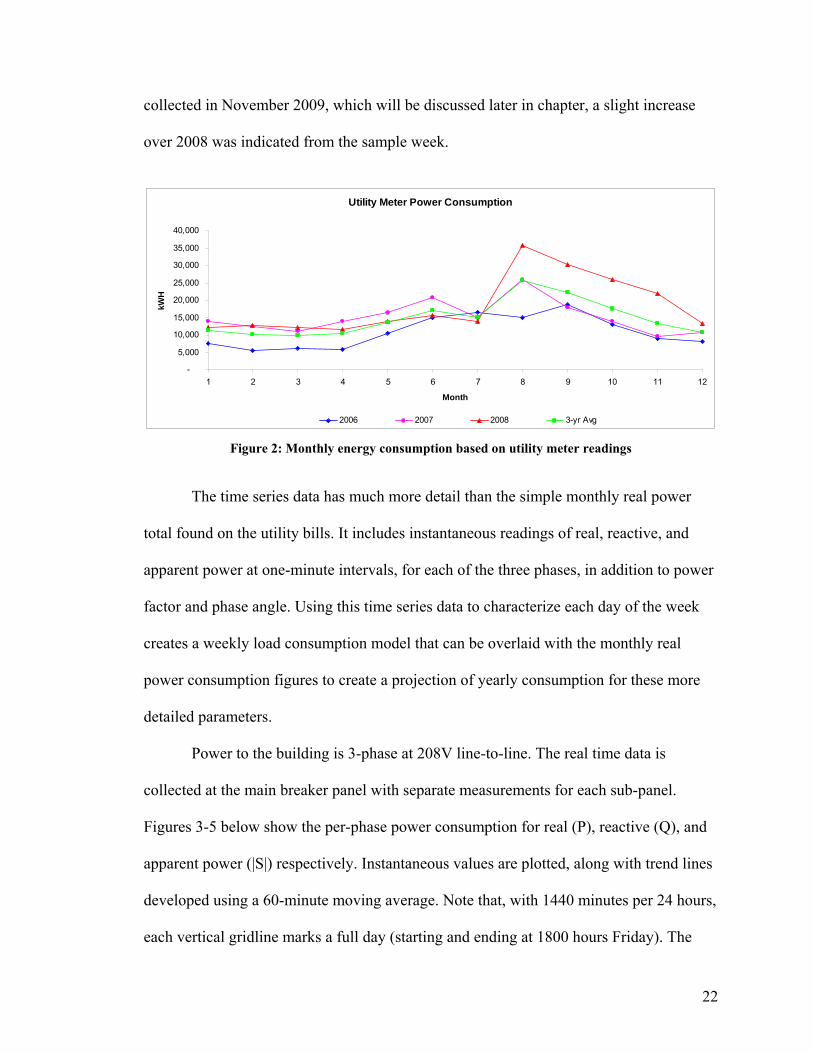
This is also apparent in Figure 6 below which shows the sum of the three phases
for real power and reactive power. Instantaneous values are plotted, along with trend
lines developed using a 60-minute moving average. To determine the total power needs
for the building, all three phases are added together. The total per-minute power of each
type was calculated for each phase and then the phases were added together.
On the graph it is clearly seen that the real power is of much greater magnitude
than the reactive power, indicating that the apparent power and real power plots would be
very similar. This further illustrates the previous discussion about their similarity due to
the nearly-ideal power factor.
Total 3-phase powers: P, Q
-10000
0
10000
20000
30000
40000
50000
60000
70000
80000
0 1440 2880 4320 5760 7200 8640 10080
Minutes (starting @ 1800 Friday)
VA
R :
W
P Real Pwr (W) Q Reactive Pwr (VAR) P Real Pwr (60 min Mov. Avg.) Q Reactive Pwr (60 min Mov. Avg.)
Figure 6: Weekly profile of power consumption from time series data
The total apparent power was used to provide the series of power consumption
values for each minute of the week in the load profile data files. This became the basis for
the total power consumption model used in the source/load power balance analysis.
26

3.2.2 Seasonal and Annual Variation
As there were incremental changes in the historical consumption data from year to
year, it is reasonable to assume that future years would also experience similar change.
The little data available for 2009 did not provide compelling evidence to steer the
decision. This was considered by involved parties and it was agreed upon to sustain this
assumption for the sake of simplicity, based on the expectation that the C&CC building’s
usage was expected to follow past trends, ignoring any dramatic change in climate. As
such, it was decided to use a three-year average to provide the projected data for 2010,
the year under study.
Cooling and heating portions of the total load also evolve with the seasons. As
shown by the historical billing data in Figure 2, each month has its own typical
consumption profile in comparison to other months. One would assume that the weather
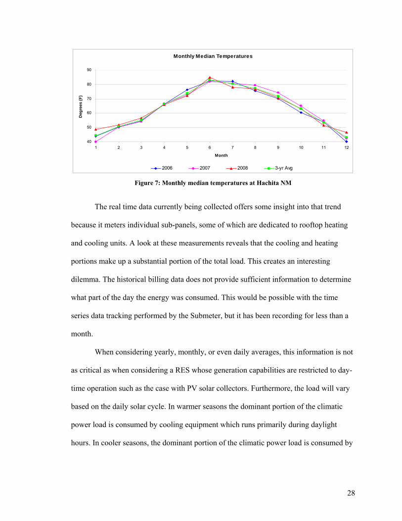
trends would have meaningful impact on this. As shown in Figure 7 below, median
temperatures for nearby Hachita NM [26], which is of similar geography and located at
similar elevation and latitude to Playas in the next valley to the east, show trends for
warmer summer and cooler winter months, as expected. Comparing this plot to the
consumption plot in Figure 2 allows for consideration of the potential impact of seasonal
temperatures on the electric loads for heating and cooling. Consumption is higher during
hot summer months than the cooler winter months. However, the consumption history
does not appear to correlate directly with the historical temperature profile from year to
year. More data on the building usage would be necessary to determine the nature of the
fluctuations.
27
Monthly Median Temperatures
40
50
60
70
80
90
1 2 3 4 5 6 7 8 9 10 11 1
Month
Deg
rees
(F
)
2
2006 2007 2008 3-yr Avg
Figure 7: Monthly median temperatures at Hachita NM
The real time data currently being collected offers some insight into that trend
because it meters individual sub-panels, some of which are dedicated to rooftop heating
and cooling units. A look at these measurements reveals that the cooling and heating
portions make up a substantial portion of the total load. This creates an interesting
dilemma. The historical billing data does not provide sufficient information to determine
what part of the day the energy was consumed. This would be possible with the time
series data tracking performed by the Submeter, but it has been recording for less than a
month.
When considering yearly, monthly, or even daily averages, this information is not
as critical as when considering a RES whose generation capabilities are restricted to day-
time operation such as the case with PV solar collectors. Furthermore, the load will vary
based on the daily solar cycle. In warmer seasons the dominant portion of the climatic
power load is consumed by cooling equipment which runs primarily during daylight
hours. In cooler seasons, the dominant portion of the climatic power load is consumed by
28

heating equipment which runs primarily at night, and likely with a substantially different
power factor.
Given the importance of these dynamic interactions, power balance must be
evaluated by the hour or even by the minute, in order to predict when the PV array will
produce energy, and how much, and when the loads will be most active. For a truly
accurate annual load profile, time series data would need to be collected over an entire
year. However, time series data for this project is only available for one recent sample
week, recorded in November, a relatively temperate month in southern New Mexico. It is
expected that there is more balance between heating and cooling loads during this month
than during the months of more extreme outdoor temperatures. Therefore, there is a good
probability that the time series data does not provide adequate information to generate a
comprehensive annual profile without making some assumptions. Therefore, the annual
load profile will be based on the distribution of power usage throughout the sample week,
repeating it for all 52 weeks of the year. It is expected that fluctuations of load timing
throughout the year will vary with the weather of the seasons. Annual temperature trends
for the period covered by the historical power bills differ by an average of 6%, so this
may introduce one of the more significant sources of error in this study.
3.2.3 Projected Annual Load Profile
Combining the historical billing data with the week of detailed time series data
creates a comprehensive annual consumption profile. The first step was to use the
monthly real power metered figures from the bills to determine what proportion of a
yearly energy load was consumed in each month. This would provide data for how to
weigh each week in the annual profile relative to each other. The week of time series data
29

was then analyzed to determine how much of a typical week’s total apparent power
consumption occurred during each minute of the week. This created a unit-less
proportion figure for each of the 10080 minutes of the week that quantifies how much of
the week’s total power was consumed during each minute. Then, by using the real power
proportional figures from the bills, each week was scaled to its appropriate portion of the
annual expected total consumption for real power. In the end, by comparing those per-
minute quantities to the source production for each minute, we are able to determine how
much energy is used from (or returned to) the grid for any given minute of the year.
Months have a variety of lengths, which results in three different numbers of minutes per
month. For months with 31, 30, and 28 days there are 44640, 43200, and 40320 minutes,
respectively.
The quantities computed per minute for a year are real power values, measured in
kilowatts. They were originally determined using the apparent power values from the
week of test data, but since the load was determined to have a power factor very close to
ideal, as discussed previously, the result would have been within 1% if the real power
values had been used instead.
3.3 Source Characterization
3.3.1 Solar Radiation and the CPV System
The basics of harnessing solar energy center around a transducer, the photovoltaic
(PV) cell, which converts solar radiation into electricity. Solar radiation is measured in
watts per square meter, and the exposure level at any particular location is dependent on
the angle of the sun in the sky, atmospheric conditions, altitude, and other parameters
[15]. Solar intensity at this project’s installation site varies between zero (when the sun is
30

not present in the sky) and upwards of 900 or even 1000 W/m2 in some conditions [27].
Determining how much electricity a particular solar panel will convert is a function of its
efficiency and the radiation to which it is exposed. Because of the lens array design, this
panel design benefits negligibly from indirect sunlight, which conveniently simplifies the
conversion projections by allowing for consideration of only the direct normal irradiance
which is the sunlight component pointing directly along the path between the sun and the
panel. Other irradiance values can therefore be ignored in the projection algorithm.
The Emcore Concentrator Photovoltaic Array (CPV) is a special type of PV
panel. As mentioned earlier, it uses Fresnel lenses to concentrate a large exposure area to
a much smaller PV cell, thus increasing the output of the cell to many times the normal
for a non-concentrating panel. As seen in Figure 8 below, the panel is built from ten
smaller arrays of approximately 200 cells each. Fairly large and heavy for a post-mounted
panel, it measures 1814 cm (~60 feet) wide by 790 cm (~26 feet) tall. It weighs 8620 kg
(~19,000 pounds—nearly ten tons). The panel has sun tracking control software to ensure
that it is perpendicularly exposed to maximum direct sunlight at all times. Extreme
precision is necessary for optimal electricity production. A deviation of as little as one
degree from the ideal angle can degrade production by up to fifteen percent. The
trajectory it follows is programmed using astronomical data. Periodically it also runs an
accuracy-check procedure where it adjusts the panel’s angle while monitoring power
output to determine whether it is actually pointing in the most advantageous direction.
Unfortunately that data is not used to correct the tracking path if it is not ideal. The array
includes a power electronics system to manage AC inversion and other parameters for
optimal power output [24].
31

Figure 8: Emcore Concentrator Photovoltaic Array [24]
3.3.2 CPV Characterization
Rated maximum power output for the CPV under standard operating conditions is
25 kW. According to the specification sheet this is temperature dependent, but
calculations on the data provided for the temperature extremes at the installation site
suggest a maximum power loss of 2% (at 122° F) and even lower loss at more common
temperatures (1.2% at 104° F and 0.4% at 50° F) [24]. Consideration of the spec sheet
data is good for a brief introduction to the unit, but there is a better source of that
information for the purposes of this project. A performance test of a sample unit was
executed in Albuquerque which provides experimental data for local performance.
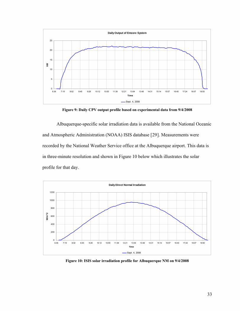
A data set was provided by the Playas site team that cataloged the power output of
the CPV panel for the daylight hours of September 4, 2008 [28]. The data is highly
detailed with three to four samples per minute, as shown in Figure 9 below.
32
Daily Output of Emcore System
0
5
10
15
20
25
6:36 7:19 8:02 8:45 9:28 10:12 10:55 11:38 12:21 13:04 13:48 14:31 15:14 15:57 16:40 17:24 18:07 18:50
Time
kW
Sept. 4, 2008 Figure 9: Daily CPV output profile based on experimental data from 9/4/2008
Albuquerque-specific solar irradiation data is available from the National Oceanic
and Atmospheric Administration (NOAA) ISIS database [29]. Measurements were
recorded by the National Weather Service office at the Albuquerque airport. This data is
in three-minute resolution and shown in Figure 10 below which illustrates the solar
profile for that day.
Daily Direct Normal Irradiation
0
200
400
600
800
1000
1200
6:36 7:19 8:02 8:45 9:28 10:12 10:55 11:38 12:21 13:04 13:48 14:31 15:14 15:57 16:40 17:24 18:07 18:50
Time
W/m
^2
Sept. 4, 2008 Figure 10: ISIS solar irradiation profile for Albuquerque NM on 9/4/2008
33
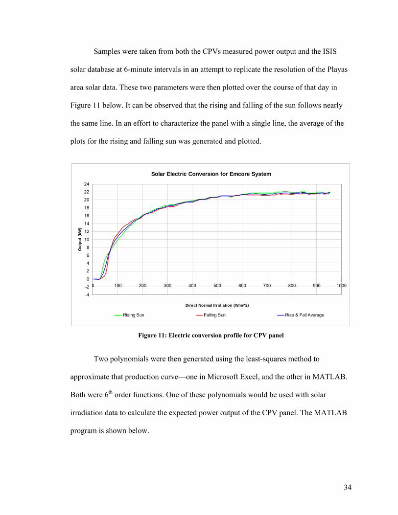
Samples were taken from both the CPVs measured power output and the ISIS
solar database at 6-minute intervals in an attempt to replicate the resolution of the Playas
area solar data. These two parameters were then plotted over the course of that day in
Figure 11 below. It can be observed that the rising and falling of the sun follows nearly
the same line. In an effort to characterize the panel with a single line, the average of the
plots for the rising and falling sun was generated and plotted.
Solar Electric Conversion for Emcore System
-4
-2
0
2
4
6
8
10
12
14
16
18
20
22
24
0 100 200 300 400 500 600 700 800 900 1000
Direct Normal Irridiation (W/m^2)
Ou
tpu
t (k
W)
Rising Sun Falling Sun Rise & Fall Average
Figure 11: Electric conversion profile for CPV panel
Two polynomials were then generated using the least-squares method to
approximate that production curve—one in Microsoft Excel, and the other in MATLAB.
Both were 6th order functions. One of these polynomials would be used with solar
irradiation data to calculate the expected power output of the CPV panel. The MATLAB
program is shown below.
34

1 data = csvread ('SolarVsPowerOutputData.csv'); 2 x = data(:,1); 3 y = data(:,2); 4 polyfit (x,y,6)
The results generated by the program, shown below, are the coefficients of the
polynomial in the following form, where the independent variable x is the solar intensity
and the dependent variable Y is the CPV power output.
Y = Ax6 + Bx5 + Cx4 + Dx3 + Ex2 + Fx + G A = 382.4216e-018 B = -924.5694e-015 C = 616.3000e-012 D = 138.0168e-009 E = -332.3873e-006 F = 144.5586e-003 G = -1.5323e+000
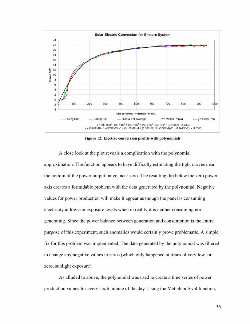
Both polynomial curves were plotted on the graph as well as seen in Figure 12
below. Excel can calculate polynomial fits up to the sixth-order. MATLAB can plot
higher-order polynomials with the Polyfit function [30], but experimentation with
various orders resulted in a best fit at the sixth order. Higher order polynomials fit the
curved portions quite well, but had unsuitable anomalies in the flattening horizontal
portion. The sixth-order polynomials generated by both tools are so similar that they print
precisely on top of each other on the plot. Since Matlab was to be used for the
characterization calculations later, its polynomial was chosen for the job to simplify the
computations.
35
Solar Electric Conversion for Emcore System
y = (4E-16)x6 - (9E-13)x5 + (6E-10)x4 + (1E-07)x3 - (3E-4)x2 + (0.1446)x - (1.5323)Y = (3.82E-16)x6 - (9.24E-13)x5 + (6.16E-10)x4 + (1.38E-07)x3 - (3.32E-4)x2 + (0.1446E-1)x - (1.5323)
-4
-2
0
2
4
6
8
10
12
14
16
18
20
22
24
0 100 200 300 400 500 600 700 800 900 1000
Direct Normal Irridiation (W/m^2)
Ou
tpu
t (k
W)
Rising Sun Falling Sun Rise & Fall Average Y = Matlab Polyval y = Excel Poly
Figure 12: Electric conversion profile with polynomials
A close look at the plot reveals a complication with the polynomial
approximation. The function appears to have difficulty estimating the tight curves near
the bottom of the power output range, near zero. The resulting dip below the zero power
axis creates a formidable problem with the data generated by the polynomial. Negative
values for power production will make it appear as though the panel is consuming
electricity at low sun exposure levels when in reality it is neither consuming nor
generating. Since the power balance between generation and consumption is the entire
purpose of this experiment, such anomalies would certainly prove problematic. A simple
fix for this problem was implemented. The data generated by the polynomial was filtered
to change any negative values to zeros (which only happened at times of very low, or
zero, sunlight exposure).
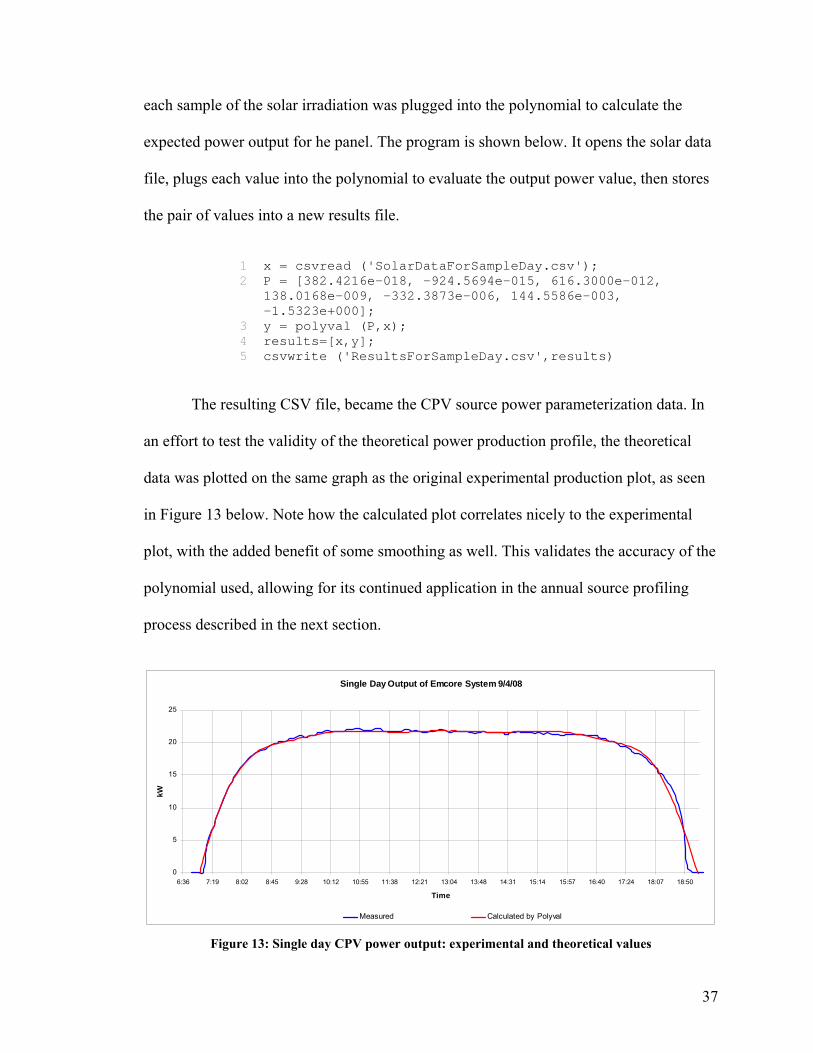
As alluded to above, the polynomial was used to create a time series of power
production values for every sixth minute of the day. Using the Matlab polyval function,
36
each sample of the solar irradiation was plugged into the polynomial to calculate the
expected power output for he panel. The program is shown below. It opens the solar data
file, plugs each value into the polynomial to evaluate the output power value, then stores
the pair of values into a new results file.
1 x = csvread ('SolarDataForSampleDay.csv'); 2 P = [382.4216e-018, -924.5694e-015, 616.3000e-012,
138.0168e-009, -332.3873e-006, 144.5586e-003, -1.5323e+000];
3 y = polyval (P,x); 4 results=[x,y]; 5 csvwrite ('ResultsForSampleDay.csv',results)
The resulting CSV file, became the CPV source power parameterization data. In
an effort to test the validity of the theoretical power production profile, the theoretical
data was plotted on the same graph as the original experimental production plot, as seen
in Figure 13 below. Note how the calculated plot correlates nicely to the experimental
plot, with the added benefit of some smoothing as well. This validates the accuracy of the
polynomial used, allowing for its continued application in the annual source profiling
process described in the next section.
Single Day Output of Emcore System 9/4/08
0
5
10
15
20
25
6:36 7:19 8:02 8:45 9:28 10:12 10:55 11:38 12:21 13:04 13:48 14:31 15:14 15:57 16:40 17:24 18:07 18:50
Time
kW
Measured Calculated by Polyval Figure 13: Single day CPV power output: experimental and theoretical values
37

3.3.3 Solar Irradiation Profile for the Installation Site
Estimating conversion of solar energy to electricity is dependent upon the pattern
of solar radiation at the installation site. There are sources of geographical information
available that can predict the sun’s trajectory and provide solar intensity projections. One
such example considered for this study is the Bird Clear Sky Model developed by the
Solar Energy Research Institute (SERI) [31, 32]. This spreadsheet-based tool calculates
the solar radiation projections based on a number of user-defined parameters such as
geographical coordinates, altitude (by using the nominal atmospheric pressure), moisture
(indicated by the total moisture in a vertical column), and others. The solar data was
compiled using as many of these parameters as possible using various geographical
information sources [33, 34], and utilizing the provided defaults for parameters that were
not readily available. The computed results were saved for later comparison against other
options. The problem with using this calculator is that it provides an estimation of clear-
sky radiation and does not offer any simulation of weather patterns that are sure to impact
real-world conditions at the site. While New Mexico is a predominantly sunny state with
more than 300 days of sunshine per year, assuming the site would experience no solar-
compromising weather at all would likely introduce a substantial source of error in the
analysis.
Because of such concerns, the solar radiation information would ideally come
from historical data collected at the location where the CPV array would be installed.
Unfortunately no such local data was available for this study. However, there are a
number of databases that catalog such information for a variety of sites across the USA
38

and elsewhere. The ideal sample site would be as close to the installation site as possible,
and share maximum similarity in daily solar trajectory.
Closest available solar profile
Two locations relatively similar to the installation site were identified using the
Cooperative Network for Renewable Resource Measurements (CONFRRM) database
[27]. Both of the chosen sites (seen in Figure 14 below) were within reasonable proximity
to the installation site, one located 173 km to the northeast in Las Cruces, NM, and the
other 201 km to the east in El Paso, TX [35, 36]. Both collection sites are similar to the
Playas elevation of 1371 meters, at 1201 and 1219 meters, respectively. A key indicator
for a site with similar solar exposure is latitude. Drawing a vector from Playas to each
potential data collection site, the Las Cruces site’s latitude displacement component
points 24 km north of Playas, whereas the El Paso site is 8 km south, suggesting it would
have a more similar solar profile.
Figure 14: Map of Playas NM region [37]
39

Validating usage of closest data
Assuming that a closer latitude match would result in a more similar day length,
astronomical data from the National Oceanic and Atmospheric Administration (NOAA)
was considered. The NOAA sunrise and sunset calculator [38] was used to determine the
times of sunrise and sunset at Playas and the two other locations. This information was
used to compute the length of the day at each site on four sample dates spread throughout
1999, the one full year that historical data was available for both sites. The summer and
winter solstices and vernal and autumnal equinoxes were chosen as comparison dates
since they offer both the extreme cases of day/night proportion and the equilibrium
points, and they are distributed evenly throughout the solar calendar.
Compared to the data for Playas, the Las Cruces site had matching day length for
the equinoxes and a difference of +2 minutes and -2 minutes for the summer and winter
solstices respectively. The El Paso data had matching lengths for both solstices and the
autumnal equinox, with a +1 minute difference on the vernal equinox. By this
comparison it appears that either choice would be reasonably similar to the Playas site.
Las Cruces had larger deviations, but since one is positive and the other equally negative,
they would likely offset each other over the course of the year. The El Paso site deviated
on only one comparison day, and by only one minute, but the unbalanced nature suggests
it might be slightly less comparable despite the smaller difference. In either case, the
sample sites had worst-case day length differences of less than a half percent of the total
day length. The Bird Clear-sky Model irradiation results were equal to or slightly higher
than either site, confirming that, with occasional cloudiness, the site data was realistic.
The Las Cruces data was ultimately chosen as the best comparison. Its day length
deviation had a balanced offset, and it was located closer to the Playas site. Furthermore,
40

there was an additional swaying factor. The data collected in Las Cruces included
additional measurements for wind speed and direction, which the El Paso data did not.
These parameters were not specifically needed for this study, but if later work were to be
done on this project, or at the same site, that might be able to take advantage of the extra
data, its availability could be advantageous.
The data came in the form of comma-separated value (CSV) files, one per month,
for the year 1999 which was the most recent year that there was data for every month.
There are several solar measurements included in the data but, as mentioned earlier, only
the direct normal irradiance is relevant for the design of solar panel in use for this project.
Measurements were taken every five minutes for the entire year. Ten of the monthly files
were fully complete, but the months of January and July were missing a total of three
periods of approximately 62, 72, and 96 hours. The CSV files from January 2000 and
July 1998 were used to replace missing data for the same dates and times in 1999. The
choice of a single year for this data is not ideal. It likely would have been better to use
some combination of years to minimize the impact of a particular year’s weather trends,
but data for locations this close to the isolated installation site is hard to come by and the
available data sets have limited time coverage. Regardless, it was assumed that data
which incorporates at least some kind of weather impact would be better than the Bird
calculator that assumes 100% sunshine every day.
3.3.4 Projected Annual Solar Source Profile
The first step in creating the annual conversion projections was to get the solar
data into the same resolution as the load data. The load data was at one-minute resolution
which was worth preserving for maximum accuracy in the dynamic source/load
41

interaction in the power balance profile. Therefore, rather than averaging the load data
from one to five minute resolution, the solar data was expanded from five to one minute
resolution. The intermediate data was interpolated a linear progression between existing
values. This provided a smoother transition between known values than the stepped
progression that would have resulted from repeating each value five times.
Similar to the characterization process for the CPV panel mentioned earlier, the
same polynomial equation was used to create a time series of power production values for
every minute of the year. Using the Matlab Polyval function, each month’s solar
irradiation CSV file was opened, each value was plugged into the polynomial which
generated a power output figure for that irradiation value, and the resulting data was
stored in a new CSV file.
The resulting files became the CPV source power parameterization data for the
entire year. They are the same sizes as their corresponding monthly load profile files so
that computations can be performed on them in pairs during the analysis stage, as
explained in the next section.
3.4 Analysis
3.4.1 Overview
There are four main functions of the overall analysis:
A. Perform the calculations and plots necessary for technical characterization of the
inputs, which in this case are the system components and variables that affect
them. This has already been performed and described above. The Emcore CPV
source and C&CC building load are characterized to one-minute resolution for an
entire year.
42

B. Compute the interaction of the components and display the results. This is where
a mathematical engine is applied to the data inputs to determine the power
balance between source and load for each minute of the year, and the results are
displayed in a clear format for the user to review, along with other considerations
such as financial and environmental factors. This will be performed three times to
calculate results for the integration of one, two, or three CPV panels.
C. Allow the user to adjust parameters and observe the resulting effects. In this
portion the user will be able to adjust constants and recalculate various values that
relate to the energy costs, net metering and renewable energy credit programs,
project term and financing options. The results will update accordingly so the user
can evaluate the implications of various parameters.
D. Provide meaningful information to assist the user in evaluating the various
options and making system design choices.
3.4.2 Tools
Now that the needs have been defined, and much of the preparation work has
been completed, it is necessary to evaluate the possible options for the decision support
analysis tool(s) that will be most advantageous for this application. As discussed
previously, there are two leading contenders among the existing simulation packages,
plus the remaining third option to create one from scratch. However, since so much work
has already been done to characterize the load and source, some of the difficult analysis,
for which the existing tools are typically helpful, will not need to be performed. In fact,
since that is a major component of what those packages do, it is safe to say that much of
43

their capability will not need to be utilized. Furthermore there are some other factors that
make the existing choices less attractive.
First of all, both HOMER and Hybrid2 are meant to characterize a system from
the ground up and help the user make choices between various types and quantities of
system components. This project differs in that it aims to evaluate a particular system
setup (albeit at three different quantities of the same source). Secondly, the existing
packages favor the use of traditional PV equipment. The CPV array behaves quite
differently, so traditional PV conversion profiles used by existing software packages can
not be expected to characterize the CPV accurately. HOMER offers the capability to
provide custom characterizations for wind turbines and other energy sources, but the PV
source module does not offer much beyond simple specifications found only on
traditional PV panels Therefore, it would be very difficult to customize it to this
application.
Additionally, the data compiled for this project is in much greater detail than
those programs typically handle. HOMER is built around using and generating data at
one-hour resolution. Clearly it is meant for looking at the bigger picture of performance
over years or decades. This study is aimed at understanding the performance of the
system on a per-minute basis.
Finally, the energy industry currently offers a variety of renewable energy
programs that consumers can take advantage of. Some of these involve net metering at an
even exchange, others buy and sell electricity from the consumer at different rates, and
some also offer to buy renewable energy credits from customers that generate and use
their own electricity. (Yes, it is possible to get paid for electricity that never goes into the
44

grid.) PNM, the largest power utility in New Mexico offers one such program [39].
Existing tools have the capability to handle the first two of these examples, but no
available option was found that could accommodate the third possibility of including
renewable energy credit income into the financial projections for the system.
While these issues do not necessarily indicate shortcomings in the existing tools,
they do suggest an incompatibility with the goals and needs of this study. Therefore it is
prudent to consider a custom solution that is more directed toward the specifics of the
work being conducted. Since characterization of the source and load has already been
performed, a large portion of the simulation tool’s task is already completed. The
remaining parts would be to perform the power balance analysis and summarize the input
and output data in an interactive interface, which is not necessarily the largest part of the
project. MATLAB and Microsoft Excel have already been used extensively in the study
so far, and offer highly convenient mathematical tools that can be used to perform the
remainder of the analysis tasks. Furthermore, the data being used is already in formats
that were created by these programs, and the principle investigator in the study is
adequately proficient in both to use them effectively and efficiently. It is therefore a fairly
straightforward decision to create a custom analysis tool for this application.
3.4.3 Computation
Analysis of the power system actually involves relatively simple calculations. The
difficulty lies in the sheer quantity of data. The source and load profiles are characterized
at one-minute resolution, which is of great benefit to the detail level of the study.
However, there are 525,500 minutes in a year. Dealing with data files that contain more
than a half million values is relatively cumbersome. The upper limit for rows in an Excel
45

file is 65,000. It is possible to create CSV files larger than that, but the problem of how to
view them conveniently would remain. Despite the added convenience that would be
gained by using a single data file for each (source and load) profile, it was determined
such large files would be overly difficult to manage. The chosen solution was to keep the
data organized by month, which meant that there would be 24 files in total for the input
data (12 each for source and load), and twelve files for the output. Actually a total of 36
output files would be generated because the simulation was run three times to simulate
one, two, and three connected CPV panels. While the logistics were time consuming, the
files were of manageable size and error checking remained relatively simple.
The monthly source data and load data contained various quantities of values
depending on the length of the month. These quantities were used as a check to be sure
each file was the proper length and that when computed the source and load data array
sizes matched appropriately. This also helped to ensure that the proper files were being
used for each computational step. Furthermore, the output file sizes were correlated to the
input file sizes as an additional indicator of properly matched data arrays.
The fundamental calculation involved is to perform a power balance check for
each minute of the year. Essentially this means that the source power was subtracted from
the load power on a minute-by-minute basis. A positive result indicates that the load
power demand is larger than the power coming from the source and results in that
quantity of power being drawn from the electric utility grid, which is referred to in this
study as “deficit power.” A negative result indicates that the source is producing more
power than the load is consuming. This is “surplus power” that could be stored on site if
such components were included in the system. Since that is not the case for this project,
46

the extra energy will be net metered back to the grid. In cases where the purchase and
sale price of net metered energy is the same, this can be thought of as ‘storing’ the
electricity on the grid for later retrieval. The energy is not actually being stored, but the
net effect is the same. In reality it is being deposited into the grid for immediate use
elsewhere, and when an equivalent amount of new energy is used from the grid later it is
thought of as being retrieved.
To preserve the per-minute dynamic, these positive and negative values could not
simply be added up over time to determine the total amount of power used from the grid.
Instead the positive and negative values would need to be added independently to
generate separate total watt-minute values for deficit and surplus energy (later converted
to kWH). Maintaining the separation is important because it allows the analysis stage to
evaluate the earning potential for the surplus energy, to calculate possible renewable
energy credits, and to determine how much timing mismatch there is between when
power is being generated and when it is being consumed.
With these constraints in mind, a MATLAB program was written to perform the
computation. It is remarkably simple. It first loads each monthly data input file into a
1xN array of values where N is the number of minutes in the month (lines 1 and 2 of the
program below). It multiplies each row in the source file by the corresponding row in the
load file (line 3 below). Finally it writes the result to a new power balance output data file
(line 4 below). This shows the program as run for the month of January, as indicated by
the “01” designator at the end of each file name.
1 source = csvread('SourceDataMonth01.csv'); 2 load = csvread('LoadDataMonth01.csv'); 3 powerbalance = load – 1*source; 4 csvwrite('PowerBalanceDataMonth01.csv',powerbalance);
47
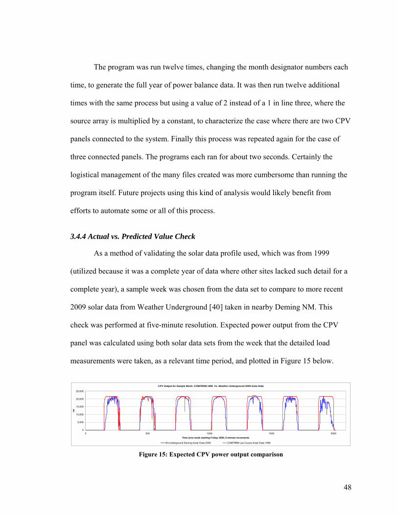
The program was run twelve times, changing the month designator numbers each
time, to generate the full year of power balance data. It was then run twelve additional
times with the same process but using a value of 2 instead of a 1 in line three, where the
source array is multiplied by a constant, to characterize the case where there are two CPV
panels connected to the system. Finally this process was repeated again for the case of
three connected panels. The programs each ran for about two seconds. Certainly the
logistical management of the many files created was more cumbersome than running the
program itself. Future projects using this kind of analysis would likely benefit from
efforts to automate some or all of this process.
3.4.4 Actual vs. Predicted Value Check
As a method of validating the solar data profile used, which was from 1999
(utilized because it was a complete year of data where other sites lacked such detail for a
complete year), a sample week was chosen from the data set to compare to more recent
2009 solar data from Weather Underground [40] taken in nearby Deming NM. This
check was performed at five-minute resolution. Expected power output from the CPV
panel was calculated using both solar data sets from the week that the detailed load
measurements were taken, as a relevant time period, and plotted in Figure 15 below.
CPV Output for Sample Week: CONFRRM 1999 Vs. Weather Underground 2009 Solar Data
0
5,000
10,000
15,000
20,000
25,000
0 500 1000 1500 2000
Time (one week starting Friday 1800, 5-minute increments
kW
Wx Underground Deming Solar Data 2009 CONFRRM Las Cruces Solar Data 1999 Figure 15: Expected CPV power output comparison
48
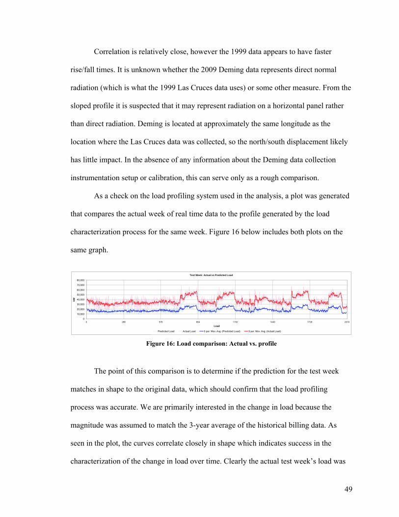
Correlation is relatively close, however the 1999 data appears to have faster
rise/fall times. It is unknown whether the 2009 Deming data represents direct normal
radiation (which is what the 1999 Las Cruces data uses) or some other measure. From the
sloped profile it is suspected that it may represent radiation on a horizontal panel rather
than direct radiation. Deming is located at approximately the same longitude as the
location where the Las Cruces data was collected, so the north/south displacement likely
has little impact. In the absence of any information about the Deming data collection
instrumentation setup or calibration, this can serve only as a rough comparison.
As a check on the load profiling system used in the analysis, a plot was generated
that compares the actual week of real time data to the profile generated by the load
characterization process for the same week. Figure 16 below includes both plots on the
same graph.
Test Week: Actual vs Predicted Load
0
10,000
20,000
30,000
40,000
50,000
60,000
70,000
80,000
0 288 576 864 1152 1440 1728 2016
Load
kW
Predicted Load Actual Load 5 per. Mov. Avg. (Predicted Load) 5 per. Mov. Avg. (Actual Load) Figure 16: Load comparison: Actual vs. profile
The point of this comparison is to determine if the prediction for the test week
matches in shape to the original data, which should confirm that the load profiling
process was accurate. We are primarily interested in the change in load because the
magnitude was assumed to match the 3-year average of the historical billing data. As
seen in the plot, the curves correlate closely in shape which indicates success in the
characterization of the change in load over time. Clearly the actual test week’s load was
49

of higher magnitude, and until more recent data can be assembled it is unknown if that is
a general trend or not.
Another data check of interest involves comparing the power balance plots (again,
for the test week) of the profiled source and load data against the actual source and load
data. This generates a plot for the week of profile data using with the profiled solar
source from 1999 in Las Cruces, and a separate plot for the actual load data using the
2009 solar data from Deming. These are plotted in Figures 17-18 below.
Power Balance - Using Predicted Week Load Data & 1999 Solar Data - 5 min Resolution
-20,000
-10,000
0
10,000
20,000
30,000
40,000
0 288 576 864 1152 1440 1728 2016
5-minute increments starting Friday 1800
kW
Load Source Balance 12 per. Mov. Avg. (Balance) 12 per. Mov. Avg. (Load) Figure 17: Power balance for profiled data sets
Power Balance - Using Actual Week Load Data & 2009 Solar Data - 5 min Resolution
0
10,000
20,000
30,000
40,000
50,000
60,000
0 288 576 864 1152 1440 1728 2016
5-minute increments starting Friday 1800
kW
Load Source Balance 12 per. Mov. Avg. (Balance) 12 per. Mov. Avg. (Load) Figure 18: Power balance for actual data sets
More on the power balance analysis can be found in section 3.5 where the
analysis results are discussed. For now this offers an opportunity for a first glimpse of
how the load and source will interact. Figure 17 shows some periods of negative power
balance values. These are times when the source is producing more than the load is
consuming, thereby generating a surplus. Figure 18 shows that when the load is always
greater than the source power, there is no surplus energy available for storage or net
metering back to the grid. These dynamics will be discussed more thoroughly later.
50

3.4.5 Results Interface
While that all may seem like a straightforward exercise, the substantial portion of
the analysis is processing that power balance data and presenting it in a meaningful
format. The user needs to be able to read and understand the output data, and its
implications. Furthermore, the financial and environmental calculations still need to be
made in a way that allows for user adjustment of relevant constants. Microsoft Excel was
chosen as the interface for this since it offers a convenient user interface with the
computational tools necessary to present the information in a mathematically interactive
format. In other words, the user will be able to enter the user-adjustable parameters, and
the interface will recalculate the results based on that input. This mathematically capable
interface can also be used as an effective data verification and error calculation tool.
A three-page spreadsheet was developed to perform this group of functions, one
page per panel quantity (representing one, two and three connected CPV panels). Months
of the year are represented in columns and the data and calculations are represented in
rows. Refer to Figure 19 below for a selection from the spreadsheet. Certain months have
been omitted in an effort to fit a reasonable portion of the sheet onto the page. Full-page
panel prints of the spreadsheet’s three pages can be found in the Appendix of this thesis.
51
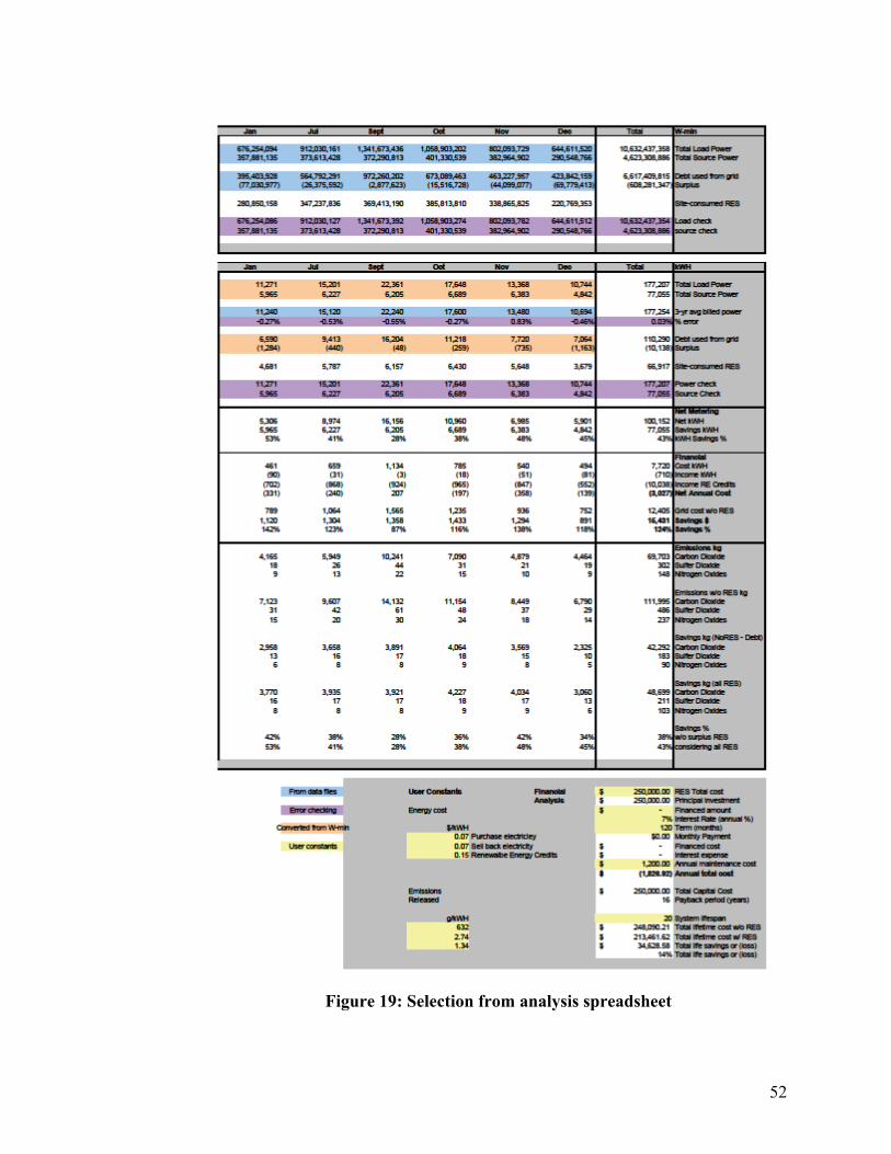
Figure 19: Selection from analysis spreadsheet
52

The first effort was to extract the sums of positive and negative power balances
from each monthly results file. The source and load power data for each month was also
summed and entered in the spreadsheet to use for error-checking. These sums were
performed separately within each data file and the values were pasted into the
spreadsheet. Again, with this file management hassle, an automated process would have
been a time saver. This data is found in the top box of the spreadsheet and comes in the
form of watt-minutes, which is not a particularly useful unit. So, a separate section of the
spreadsheet shows the same information converted into kilowatt-hours (kWH) which is
the standard unit for power utility bills, and it is more user-friendly. This is the middle
box on the sheet which contains most of the information that will interest the user.
In the middle box portion of the sheet, two important error-checking opportunities
were exploited. The power utility bill data that was originally used to project the per-
minute load profiles was retrieved. Each month’s three-year average of total kilowatt
hour consumption was entered directly into the spreadsheet in the 3-yr average billed
power row (highlighted in blue). Then, the theoretical sum of power consumed for that
month (as calculated by the load profiling process and used in the power balance
calculations) was compared to that original consumption value derived from the power
bills and a percentage error was calculated in the % error row (highlighted in purple).
This completes a critical loop of verifying whether each month’s theoretical power
consumption derived by the load profile matched the original data it was based upon.
Error was extremely low, ranging from 0.0 to 0.83%. This helps to confirm that there
were no obvious problems with the data processing that were used to create the monthly
load profiles.
53

The source profiles already had some assurance of accuracy from the comparison
made between the sample production day and the projected production computed by the
polynomial calculations. However, as an additional check, one of the monthly sums was
compared to an estimated month’s worth of CPV production, based on the test day data.
Roughly integrating the area under the Emcore daily production curve, and multiplying it
by 30 days, results in a monthly estimate of 7000 kWH for the month of September (the
same month as the one-day test was performed). Analysis results showed production of
6200 kWH, a difference of 13%. This comparison is very rough, however, because the
estimate assumes the same solar irradiation for every day of the month, but the test was
performed in the first week of September. Days get shorter as the month progresses, so
the solar irradiation, and resulting power production, should decline accordingly. Also,
the test location in Albuquerque has different solar, atmospheric, geographic and climatic
conditions than the Playas installation location for which the source profile was built.
Regardless, considering the variances in parameters which could easily cause that degree
of error, it is sufficiently low to conclude that major problems with the source profile data
are unlikely.
The remainder of the spreadsheet handles the calculation and display of energy
dynamics, financial evaluation, and environmental factors that are based on the analysis
results. The middle box contains all of the monthly information with totals in the right
column. The bottom box contains the user inputs and the lifetime financial projections for
the installation.
The center box is where most of the analysis is performed. Its top section covers
the error checking mentioned above, in addition to some calculations of power supply
54

and demand. Each column represents a month, so the figures mentioned to follow are
monthly figures. Debt used from the grid is a total of all the positive power entries in the
month’s simulation results data. This represents the total kWH of electricity drawn from
the grid. The next line Surplus RES is a sum of all the negative power entries in the
month’s simulation results data. This represents the total kWH of electricity that was
generated and unused on site. This is energy that could be stored if such capacity were
available in the system or, as in the case of this study, can be sold back to the utility via
net metering (sometimes referred to as ‘grid storage’ as explained earlier). The next row,
Site-consumed RES is the difference between total solar energy produced and the amount
of that energy that was unused on site during that month. This represents the amount of
energy that was produced and consumed on site that would not be reflected in the utility
meter. This is relevant data because some utilities offer bonus credits for this figure—
essentially they are purchasing renewable energy credits (REC) from the customer in an
effort to increase the utility’s percentage of renewable energy used on its network. There
is a row further down in the spreadsheet where this is calculated, Income REC Credits,
which multiplies that kWH figure by the user-provided per-kWH price paid by the REC
program.
The next section of the center box is where net metering is calculated. The first
row, Net kWH computes the difference between kWH drawn from and sent back to the
grid. This is the net total energy purchased from the utility that month (assuming all
surplus was net metered back to the grid). The next row Savings kWH is the difference
between the total load power consumed and the energy purchased from the utility, thus
representing the total amount of energy generated on site. This can be compared to the
55

Total RES power in the section above as a check, which matches identically for all
months. This offers reassurance that the calculations are correct so far. Finally the kWH
Savings % row indicates the percent reduction in kWH purchased from the utility as
compared to not using any RES on site
The next section of the middle box begins the financial considerations. Starting
with Cost kWH it determines the cost of all the debt power used from the grid. This is not
the net kWH amount, rather it is the cost of all the energy drawn from the grid without
considering what was sent back. This is calculated separately from the net to allow
compensation for a difference in price between purchasing and selling power through the
meter. Some utilities charge a retail rate for power delivered to the load that is higher
than the wholesale rate at which they buy it back. Therefore, the next line, Income kWH,
calculates the expected income from the kWH sent back to the utility, and Income RE
Credits calculates the earning potential of site-consumed RES for cases where there are
renewable energy credits available. The following Net row calculates the difference
between the cost and income to determine the expected utility bill for that month. Next
the cost of total power consumed by the load, Grid Cost w/o RES is calculated to
illustrate what it would have cost to serve that load without any RES. Then a difference
in cost is calculated (Savings $) and quantified by percent (Savings %). This figure is
dependent upon the price per kWH of purchasing energy and of selling it back, and any
renewable energy credits. All three of these prices are entered by the user in the bottom
box.
The final portion of the middle box calculates the emissions figures for carbon
dioxide, sulfur dioxide, and nitrogen oxides. The emissions per kWH are user constants
56

that are determined by the way power delivered to that site is produced. HOMER uses a
set of default values for this is the user does not specify [6], so for a sample case these
theoretical values were used in for lack of better data from the utility. The first group of
figures computes the total monthly emissions in kg that would result from generating the
kWH listed in Debt used from the grid which incorporates energy generated and used on
site but ignores net metered power. The next group performs the same calculation on the
total power consumed by the load as an indication of emissions in the case where no RES
are used. Savings of emissions are calculated as the difference between these two. The
next group is a calculation of total emissions assuming that the energy was net metered
back to the grid and replaced power that would have otherwise been generated by non-
renewable means. The final group of calculations in the emissions section offers two
ways to consider pollution reduction. The first case relates to emissions reduction as the
result of power generated and used on site, the second relates to emissions reduction as a
result of all RES power generated on site. Calculating both allows us to decide whether or
not to consider the emissions reductions done on behalf of other customers on the grid by
sending them energy cleanly produced by the RES.
Discussion so far on the middle box has referred exclusively to monthly figures.
The column to the right of the monthly columns totals the monthly figures into an annual
result.
The bottom box is where the user inputs are located, and where the remainder of
the financial data is calculated. Here the user provides data for energy costs and
emissions statistics, as mentioned previously. These values are hard-linked to the
underlying sheets which do all the identical calculations for the cases of using two and
57

three connected panels. It is worth noting that many power utilities have scaling rate
structures that are dependent on various consumption thresholds. Since these structures
vary from utility to utility and for the service size classification, it was decided to not
attempt to incorporate those intricacies in this computational model. The proper rates can
be estimated based on the monthly kWH consumption figures when the rate is entered by
the user, as will be done for the sample scenario discussed in the next section on output
analysis.
The remainder of this box contains a financial calculator for evaluating project
lifetime figures. The user enters the up front capital cost including installation, the
principle value and interest rate for any loan needed, annual maintenance costs, and life
span of the equipment. In some cases significant tax deductions and/or credits are
available to offset the capital costs of RES systems, but since they have relatively short
term limits and vary greatly by locale and qualifications required, they were not included
in this analysis. The spreadsheet calculates the cost of the financing, monthly payment
amount, interest expense, and generates a total annual cost including electricity bills. A
payback period is also calculated based on savings compared to a system without any
RES, and lifetime cost and savings figures in dollars and percent for the RES-integrated
system versus the grid-only system without RES. Capital costs, financing, and
maintenance costs are entered separately on each sheet to allow for the difference in the
cost for installing multiple CPV panels.
3.5 System Characterization and Output Evaluation
Evaluation of the output results is largely dependent upon the specific scenario
that is being considered. Analysis results fall into the two categories of power usage and
58

financial/environmental factors. Power usage figures are calculated before entering the
spreadsheet, so this is not a dynamic component as with the financial section where user
variables can be adjusted. These pertain to the financial aspects of the evaluation. The
variety of user-chosen variables involved can quickly create a plethora of hypothetical
options to consider. In an effort to simplify the explanation of what can be learned from
the simulator’s results, two sample scenarios will be used and evaluated for each of the
three CPV panel quantity cases. One will assume even trade net metering and the other
will add renewable energy credits to the parameters to illustrate their impact. The
resulting output will be evaluated and relevant insights will be added to illuminate
alternate possibilities when notable. Power issues will first be explored, after which the
sample financial scenario will be proposed and analyzed.
As stated, the power figures are not influenced by the user-controlled variables so
they will be inspected first. Throughout the remaining analysis, Sheet 1 will refer to the
spreadsheet page that details the case where there is a single CPV panel installed, Sheets
2 and 3 will correspond to the cases of two and three connected panels respectively which
are the second and third layered sheets in the spreadsheet. Please refer to the Appendix
for reproductions of the sheets.
The motivating factor of this study was to determine how the load and source
interact. On Sheet 1, using January as an example month, we can see that the total load
power consumed is just over 11 MWH. The total RES power produced is just under 6
MWH. The resulting power used from the grid is not simply the difference between these
two (approximately 5 MWH). Instead, because the CPV only produces electricity during
daylight hours, and it is likely to produce either more or less than the total load at any
59
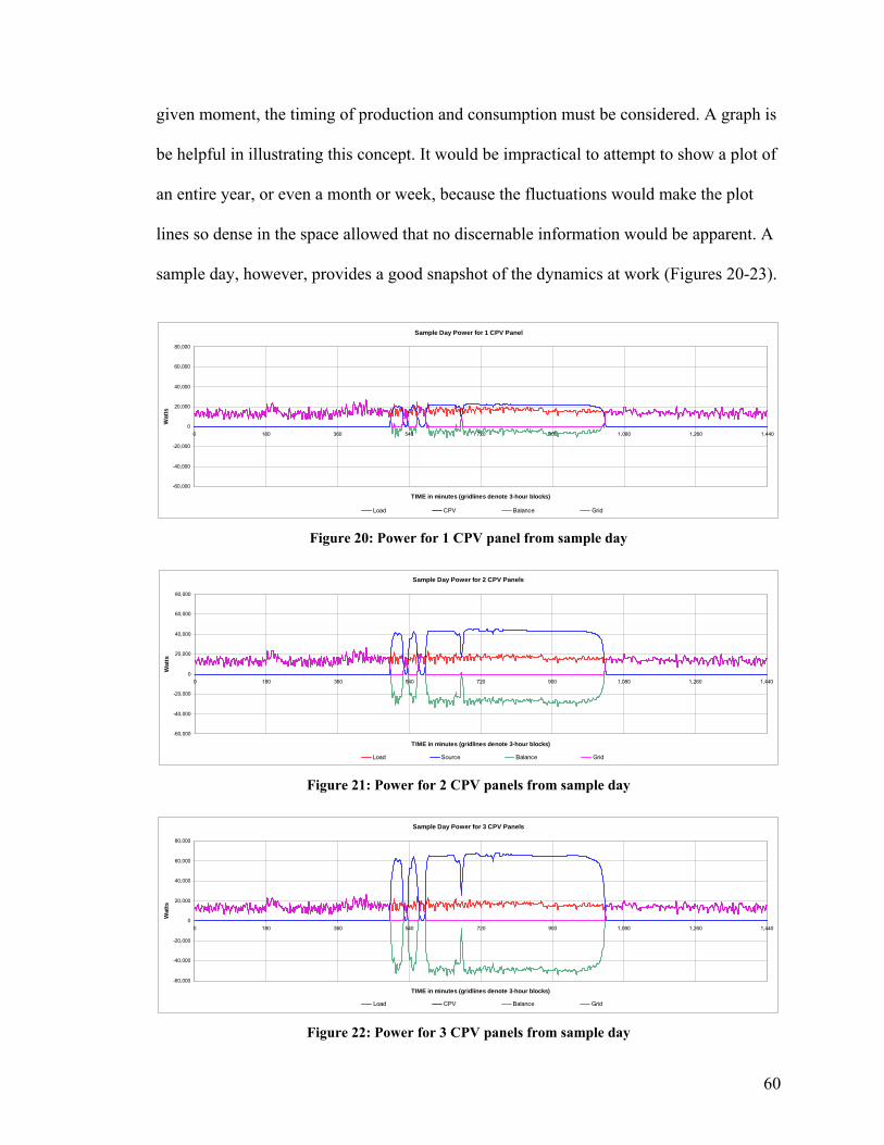
given moment, the timing of production and consumption must be considered. A graph is
be helpful in illustrating this concept. It would be impractical to attempt to show a plot of
an entire year, or even a month or week, because the fluctuations would make the plot
lines so dense in the space allowed that no discernable information would be apparent. A
sample day, however, provides a good snapshot of the dynamics at work (Figures 20-23).
Sample Day Power for 1 CPV Panel
-60,000
-40,000
-20,000
0
20,000
40,000
60,000
80,000
0 180 360 540 720 900 1,080 1,260 1,440
TIME in minutes (gridlines denote 3-hour blocks)
Wat
ts
Load CPV Balance Grid Figure 20: Power for 1 CPV panel from sample day
Sample Day Power for 2 CPV Panels
-60,000
-40,000
-20,000
0
20,000
40,000
60,000
80,000
0 180 360 540 720 900 1,080 1,260 1,440
TIME in minutes (gridlines denote 3-hour blocks)
Wat
ts
Load Source Balance Grid Figure 21: Power for 2 CPV panels from sample day
Sample Day Power for 3 CPV Panels
-60,000
-40,000
-20,000
0
20,000
40,000
60,000
80,000
0 180 360 540 720 900 1,080 1,260 1,440
TIME in minutes (gridlines denote 3-hour blocks)
Wat
ts
Load CPV Balance Grid Figure 22: Power for 3 CPV panels from sample day
60

Solar Irradiation for Sample Day
0
200
400
600
800
1000
0 180 360 540 720 900 1080 1260 1440
TIME in minutes (gridlines denote 3-hour blocks)
w/m
^2
Direct Normal Irradiance
Figure 23: Solar irradiation from sample day
The daily profile of Figures 20-23 shows minutes with vertical gridlines
indicating three hour blocks. Figure 23 is a plot of the day’s solar intensity, included for
reference, on which the mid-day low points likely indicate cloud cover. Figures 20-22
plot the power balance. In the early morning and night time hours the grid consumption,
load, and power balance are all synchronized since they are all equal. Around 8:00 AM
the blue CPV production quickly peaks as the sun rises. Dips in this plot most likely
indicate cloud cover for short periods. It drops back to zero quickly as the sun sets around
5:00 PM.
On all three plots there are times where no grid energy is being utilized, as seen
by the flat pink line on the zero axis. Not surprisingly, this occurs when the CPV is
producing more energy than the load is consuming. The green line below the axis
indicates the total quantity of surplus energy being generated but not consumed on site.
Note that none of the simulated quantities of CPV panels create a situation when the grid
connection is not utilized for at least a portion of the day. This is partly because the solar
system can not generate electricity in the dark, and partly because surplus CPV energy is
not stored locally. This explains how, at times—especially as shown on Sheets 2 and 3,
power is still being purchased from the grid even though total daily production exceeds
61

the total daily load. This indicates an opportunity to take advantage of net metering
and/or storage. On-site storage will gain more advantage over net metering if the price
paid for each kWH consumed from the grid is more expensive than the income received
per kWH delivered to the grid. On an even exchange net metering arrangement, the
storage components (and their expense) can be eliminated in preference of utilizing free
“grid storage.” In cases where renewable energy credits are available it will likely be
more financially beneficial to store on-site, but the cost of the storage components will
make that a more complex decision.
These power balance dynamics can be observed numerically on the spreadsheet in
the top portion of the middle box. In the January column on Sheet 1, the 1284 kWH of
surplus power results in a net consumption of 5306 kWH from the grid if net metering is
utilized. This results in a kWH savings of 53% over what the usage would have been
without RES connected. Similar observations can be made on Sheets 2 and 3 to find that
surplus power increases without much reduction in the monthly grid power usage, as was
attributed to night time loads not being served by the CPV.
The next section can be used to consider the costs of the energy management
decisions described above. A price of 7¢ per kWH was used in this sample case which
accounts for the 5.2¢ Large Power Service rate [41] per kWH in effect for the building,
plus approximately $100 in additional costs, which amounts to roughly 1.8¢ per kWH for
a month with January’s usage. For months where usage is higher the per kWH share of
the fixed costs would come down, but leaving the estimate at 7¢ provides a worst-case
scenario to prevent overly optimistic figures. This example also assumes even exchange
62

for net metering so the price is also set to 7¢ for the sellback rate. No renewable energy
credits are assumed, but the specific benefit thereof will be mentioned when relevant.
The financial implications of net metering for this example are a savings of $418
for a single CPV, but increase to $835 and $1746 for two and three panels. However, the
three panel system is operating in a theoretical state in that example, since the utility does
not usually purchase the power back, but rather banks it for later use. In this scenario the
banked power would accumulate faster than it can be withdrawn which does not generate
income. In this case the system would likely be switched over to another program where
the utility buys the power back at a lower wholesale rate. This situation does, however,
highlight an opportunity to consider using more of the RES generated power on-site,
perhaps to feed other nearby loads or feed it into the downstream microgrid of the town.
But that is beyond the scope of consideration here. Regardless, care must be taken when
using this spreadsheet, especially with multiple panels connected, to not rely on capital
investment payback scenarios that would require the theoretical (and unlikely) state
where the RES are making a profit. Again, buy-back figures that are set appropriately for
those other programs, if available, can alleviate this concern.
Emissions figures call attention to the environmental impact of the RES system.
Net metering and/or storing energy on site could, in this case, save 11,309 kg of carbon
dioxide emissions for January (this is approximately the amount released by burning
1000 gallons of gasoline in a typical automobile). Other pollutants are quantified here as
well. As mentioned earlier, these figures are based on the default values provided in the
HOMER simulation software. Utilities do not appear eager to release emissions
63

information since many variables impact these figures, they generally do not produce all
of the power they sell, and they may not even be able to calculate it themselves.
The final, and perhaps most useful, portion of the output analysis involves the
bottom box on the spreadsheet. This is where the lifetime cost/benefit analysis is
calculated. With a retail price of $250,000 per CPV panel, including installation, there is
a sizable capital investment required. The test case used that figure for each panel, except
the two-panel system assumes a cost of $175,000 each, which reflects a discounted price
paid for the pair being used in Playas. By these figures, the three-panel system price may
seem disproportionately high, but it is unknown whether it could have been acquired at a
discount so its price is left at normal retail. The example scenario also assumes 50% of
the project cost would be financed at 7% interest over ten years. A twenty year life span
was used as that is the minimum of the various numbers mentioned by sources consulted.
Annual maintenance costs were roughly estimated at $100 per month for an annual
expense of $1,200.
In all three panel quantity cases, the system fails to pay for itself with these
figures. For a single panel the total lifetime cost is 87% higher than what the cost of
electricity would have been without the use of RES. The two and three-panel systems
cost 92% and 241% extra. It is also noteworthy that this has not accounted for the
profitability problem discussed above.
With figures like this, one must consider what the primary motivation of the RES
system is. In the case where it is desired to help a load use as little grid energy as
possible, then the extra expense may be justifiable. If the intent was to reduce overall cost
by integrating RES, then it is not likely to be helpful in this scenario. It is worth
64

mentioning here that the price of three CPV panels could pay for half of the equipment
and installation costs of a utility-scale wind turbine rated at 1.6 megawatts. It is common
for these to generate about 1,000 kilowatts when operating, which is a scale of more than
ten times the 75 kW rating of the trio of CPVs. Wind turbines come with their own set of
logistical and regulatory challenges that are much more cumbersome than installing solar
panels, so it’s nowhere near a direct comparison, but it does offer some perspective.
There is another possible option that would provide a clear benefit. PNM, the
largest electric utility in New Mexico offers some renewable energy credit programs that
would definitely alter the outlook. These programs may also be available from utilities in
other areas. Keeping with all the same assumptions as the previous example, and
including a 15¢ REC paid to the customer for each kWH generated and used on site, we
get very different results. In this case the single panel option comes within 6% of
breaking even. Two panels saves 9% over grid-only, and the three-panel system is 139%
higher than the grid-only cost. If financing expenses are eliminated then some cost
savings start to appear, as seen in Figure 19, which shows a 14% lifetime savings for the
single panel scenario. Two panels saves 36% and three costs 79% extra.
At a grid energy price of 7¢ per kWH these systems may have a hard time paying
for themselves, especially without the REC benefit. Raising the rate to 10¢ and keeping
the REC rate at 15¢ results in a 9% savings for one panel and 32% savings for two, and
costs 58% extra for three panels, with 50% of the investment financed at 7%. Removing
the financing option again looks better for the one and two-panel systems which save 23
and 52 percent respectively. The three-panel system is still losing money, costing just
16% more than grid power alone.
65

Considering these figures, it is easy to conclude that a three-panel system is not an
advantageous option unless the customer is willing to pay extra for their clean energy or
they can get better pricing. It generates power far in excess of what can be used on-site
and thus becomes more of a miniature power plant rather than a local energy source. A
two-panel system also looks to be less financially viable than a single in some cases
depending on the financial inputs and whether the buyer can secure a discount as in the
case of the Playas application. The single panel system does show promise in paying for
itself more consistently, largely because it is more closely suited to the power needs of
the building, and puts less demand on the payback potential of net metering options.
In cases where utility power is more expensive than these test figures, the
possibilities look much more promising, especially if the up-front costs are financed at a
lower interest rate, or less money is borrowed. If the load increases significantly above
the three-year average assumed for this study (as may already be the case as shown in
Figure 18), then more of the generated power would be used on-site and more panels may
begin to appear viable, especially when revenue from renewable energy credits can be
generated. Also, if quantity discounts are available, or if co-location of multiple panels
incur lower installation costs, the figures could look better.
There are also situations where cost savings is not the primary deciding factor,
and for those cases the CPV panel may be an attractive option, such as remote areas
without grid connections, applications where there is minimal night time load such that
less power needs to be purchased, or the simple cases where the customer is willing to
pay what it costs to be green. The two-panel scenario, despite breaking even in only the
most advantageous scenarios, will spare the planet of 92,000 kg of CO2 emissions over its
66

lifetime, which is an 87% reduction when compared to grid power alone. Perhaps the
wise conclusion is that renewable energy simply costs more. This is assumed to be a
contributing factor in the advent of governmental incentives in place to encourage people
to undertake renewable energy projects.
67

CHAPTER 4 CONCLUSION
This project was successful in many ways. While it was not apparent at the outset,
the load and source characterization process constituted the bulk of the work, and a
significant part of its contribution. Much effort went into carefully considering as many
options and variables as possible to make the best possible models for future power
consumption by the load and generation by the renewable energy source/s.
Primarily, it involved the construction of large data sets for which there was little
confirmed information to start with. Building wisely from know quantities, and
interpolating, estimating, and calculating effectively, this project created impressive
results. The source characterization was closely correlated with the test that was used to
generate it, and the figures that came out after processing were in line with expectations.
The load characterization was based on a small amount of data, a single week of detailed
data from the data logging meter, combined with three years worth of very simple utility
power bills with little more than a total monthly consumption number. It too generated
results that closely correlated with expectations. The calculation engine demonstrated its
accuracy as well.
Aside from the technical success, this project made a number of valuable
contributions to the study of renewable energy systems. First of all, it provided the means
to include renewable energy credits in the financial projections. This feature is not
available in the popular existing simulation packages. There are some locales where this
68

is a significant factor and by including it in this study a door was opened to bring greater
attention to this consideration.
Characterization of the Concentrator Photovoltaic Array’s output as a function of
the solar irradiation is another important contribution. Whereas this information may be
known to the manufacturer, it was not previously available to the user and researcher. As
it is a non-traditional application of solar electricity production, modeling its conversion
provides insight that other analysis tools could not.
A thorough study of the power quality issues involved was also included in this
research, an aspect which is largely undocumented in the existing literature on the topic.
For example, by not mentioning it, a great majority of the available studies that focus on
integration of RES systems seem to assume that they will be dealing with an ideal power
factor, a fully compensated load/source, or that they do not need to consider power factor
at all. The respected off-the-shelf simulation tools used for RES system analysis also do
not include provisions for calculating or compensating the power factor. While it was
determined that power factor would not have a significant impact on the results for the
project considered by this study, in the process it did determine the necessary
considerations that would be applied in the non-ideal case. Having gone through the
exercise of making the power factor determinations appears to be uncommon among
similar projects.
The results indicate that, for the load considered, a single CPV panel can be a
beneficial addition to the commercial building’s energy system. Under various, but not
all, conditions it will be able to pay for itself and create cost savings over its lifetime.
However, results show that more panels do not add significant benefit in this situation, at
69

the simulated energy usage level. While there are cases where it can, the RES systems
under consideration in this study will not necessarily save the customer money, and more
is not necessarily better when it comes to RES components. The financial components are
based on a diverse set of variables that are difficult to work with in the hypothetical
mode, so honing the input parameters to the specific installation situation is essential to
making a financial feasibility determination. Regardless, whether the inclusion of the
CPV panels in the power system will end up saving money in the long run is not
necessarily the motivating factor of those who plan to build the system, so it is important
to recognize the other benefits.
Future efforts to carry this work forward would include a number of procedural,
improvements in addition to some additional features. For more convenient adaptation to
other projects, or to incorporate additional data as it becomes available, such as more
recent power bills and more real-time detailed power data, it would be useful to automate
more of the data processing steps. A number of cumbersome file management
components hinder the simulator’s flexibility. There are software tools within MATLAB
and elsewhere that could be implemented for an improved design. Adding the capability
to accommodate tiered utility rate structures would eliminate an estimation stage that the
user needs to compute manually. Also, the inclusion of tax credits and/or other incentives
in the financial computations would be beneficial. As this was a project meant for a
particular application, some constraints were treated as constants, but the dynamic nature
of changing rates, policy, building usage, weather, and other factors, including the desire
to apply it to other projects, offer compelling justification to revisit these topics if work
were to continue.
70

In summary, it is clear that this project successfully completed a formidable task
of accurately creating large data sets from limited starting information, for both the load
and source. The computation engine provided useful results that can be used to make
better decisions than would have been possible without the information it generated. It
determined that the CPV system in question can be a viable option for the site considered.
Additionally, it contributed insight on a number of topics not commonly addressed by
previous work.
71

APPENDIX
Full-page printouts of the evaluation spreadsheet appear on the following pages.
Spreadsheets for evaluation of one, two, and three CPV panels, respectively.
72
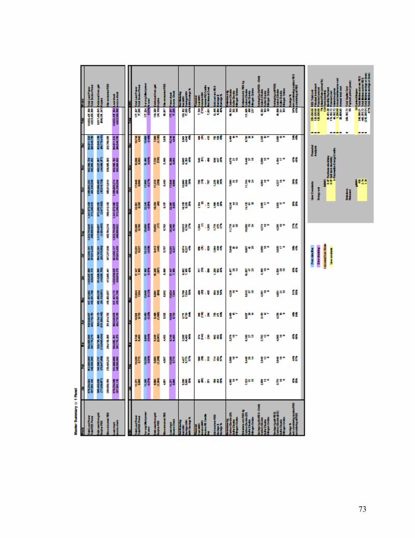
73
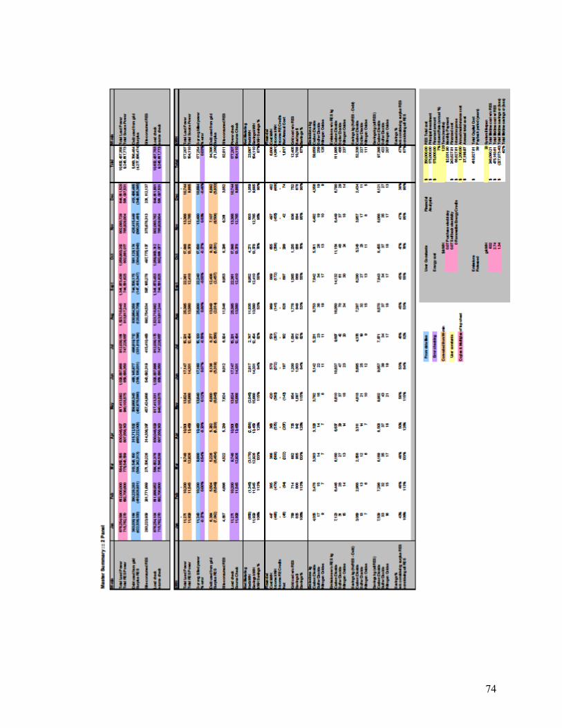
74

75

76
REFERENCES
[1] M. Hersh, “Sustainable Decision Making: The Role of Decision Support Systems,” IEEE Trans. on Man and Cybernetics-Part C. Applications and Reviews, vol. 29, no. 3, pp.395-408, August 1999.
[2] G.J. Dalton, D.A. Lockington, T.T. Baldok, “Feasibility analysis of renewable energy supply options for a grid-connected large hotel,” Renewable Energy, vol.34, pp.955-964, 2009.
[3] P. Georgilakis, “State-of-the-Art of Decision Support Systems for the Choice of Renewable Energy Sources for Energy Supply in Isolated Regions,” Int. Journal of Distributed Energy Resources, vol. 2, no. 2, pp. 129-150, 2006.
[4] P. Lilienthal, HOMER Overview, National Renewable Energy Laboratory, April, 2007, http://www.aidea.org/AEA/PDF%20files/RuralEnergyConference/HOMERIntro2007.ppt (URL).
[5] HOMER: Getting Started Guide Ver. 2.1, National Renewable Energy Laboratory, April 2005. Available: https://analysis.nrel.gov/homer/includes/downloads/HOMERGettingStarted210.pdf (URL).
[6] HOMER, Homer Energy / National Renewable Energy Laboratory. [Computer software]. Available: http://homerenergy.com/software.asp (URL).
[7] E. Ian Baring-Gould, Hybrid2: The Hybrid System Simulation Model, National Renewable Energy Laboratory, February 1998. Available: http://www.ceere.org/rerl/projects/software/hybrid2/Hy2_users_manual.pdf (URL).
[8] The Hybrid Power System Simulation Model, Renewable Energy Research Laboratory. [Hybrid2 computer software]. Available: http://www.ceere.org/rerl/rerl_hybridpower.html (URL).
[9] T. Gilver, P. Lilienthal, Using HOMER Software, NREL’s Micropower Optimization Model, to Explore the Role of Gen-sets in Small Solar Power Systems: Case Study: Sri Lanka, Technical Report NREL/TP-710-36774, National Renewable Energy Laboratory, May 2005. Available: http://www.nrel.gov/docs/fy05osti/36774.pdf (URL).
[10] M.J. Khan, “Pre-feasibility study of stand-alone hybrid energy systems for applications in Newfoundland,” Renewable Energy, vol.30, pp.835-854, 2005.
[11] C. Yue, G Yang, “Decision support system for exploiting local renewable energy sources: A case study of the Chigu area of southwestern Taiwan,” Energy Policy, vol. 35, pp. 383-394, 2007.
[12] S. Keller, S. Naciri, A. Nejmi, J. Dos Ghali, “Simulation-based decision support tool for electrification of isolated areas using a network with multiple renewable sources,” in Proc. Int. Conf. on Clean Electrical Power, Capri, Italy, 2007, pp. 1-8.

77
[13] R. Karki, R. Billington, “Considering Renewable Energy in Small Isolated Power System Expansion,” in Proc. Canadian Conf. on Electrical and Computer Engineering, Montreal, 2003, pp. 367-370.
[14] R. Billington, Bagen, “Generating Capacity Adequacy Evaluation of Small Stand-alone Power Systems Containing Solar Energy,” Reliability Engineering and System Safety, vol. 91, pp. 438-443, 2006.
[15] T. Ramachandra, J. Kumar, S Krishna, B. Shruthi, “Solar energy decision support system,” Int. Journal of Sustainable Energy, vol. 25, no. 1, pp. 33-51, March 2006.
[16] J Amador, J Dominguez, “Application of geographical information systems to rural electrification with renewable energy sources,” Renewable Energy, vol.30, pp.1897-1912, 2005.
[17] R. Karki, R. Billington, “Reliability/Cost Implications of PV and Wind Energy Utilization in Small Isolated Power Systems,” IEEE Trans. on Energy Conversion, vol. 16, no. 4, pp. 368-373, Dec. 2001.
[18] S. Youli, Z. Litifu, K/ Nagasaka, “Efficiency of Micro Grid with Storage Battery in Reliability Economy and Environment Assessments,” Int. Journal of Electrical and Power Engineering, vol. 3, no. 3, pp. 154-162, 2009.
[19] J. Manwell, J. McGowan, “Lead acid battery storage model for hybrid energy systems,” Solar Energy, vol. 50, no. 5, pp. 399-405, 1993.
[20] M. Glavin, P. Chan, “A stand-alone photovoltaic supercapacitor battery hybrid energy storage system,” in Proc. 13th Intl. Power Electronics and Motion Control Conf., 2008, pp. 1688-1695.
[21] J. Duncan Glover, Mulukutla S. Sarma, Thomas J. Overbye, Power System Analysis and Design, 4th ed., Toronto ON: Thomson Learning, 2008.
[22] EPM 4000 Sub Meter: Instruction Manual, GE Multilin, Markham ON, 2007. Available: http://www.gedigitalenergy.com/products/manuals/epm/GEK-106555H.pdf (URL).
[23] Emcore Corporation. (2009). Terrestrial Concentrator Photovoltaic Arrays [Online]. Available: http://www.emcore.com/solar_photovoltaics/terrestrial_concentrator_photovoltaic_arrays (URL).
[24] Concentrator Photovoltaic (CPV) Array, Emcore Corporation, Albuquerque, NM, 2008 [Specification sheet].
[25] RT-SVXB-EN Installation Operation Maintenance, American Standard, 2005.
[26] New Mexico Climate Center, New Mexico State University. [Online database]. Available: http://virga.nmsu.edu/cgi-shl/cns/uberpage.pl?selected=2 (URL).
[27] CONFRRM Solar Data, Renewable Resource Data Center, National Renewable Energy Laboratory, [Online database]. Available: http://rredc.nrel.gov/solar/new_data/confrrm/stdi (URL).
[28] W.D. Helgeson, Institute for Engineering Research and Applications, Albuquerque, NM, private communication, November 2009.
[29] ISIS Data, Earth System Research Laboratory, Global Monitoring Division, National Oceanic and Atmospheric Administration. [Online database]. Available: http://www.srrb.noaa.gov/isis/isispick.html (URL).

78
[30] H. Moore, MATLAB for Engineers, Upper Saddle River, NJ: Pearson Prentice Hall, 2007.
[31] R.E. Bird, R.L. Hulstrom, A Simplified Clear Sky Model for Direct and Diffuse Insolation on Horizontal Surfaces, Technical Report No. SERI/TR-642-761, Solar Energy Research Institute, Golden CO, February 1981. Available: http://rredc.nrel.gov/solar/pubs/PDFs/TR-642-761.pdf (URL).
[32] R.E. Bird. February 1991. Clearsky Broadband Solar Radiation Model [Spreadsheet]. Available: http://rredc.nrel.gov/solar/models/clearsky (URL).
[33] New Mexico Climate Summaries, Western Regional Climate Center. [Online database]. Available: http://www.wrcc.dri.edu/summary/climsmnm.html (URL).
[34] Total Precipitable Water Vapor, Drexel University, January 2006. [Online database]. Available: http://www.wrcc.dri.edu/summary/climsmnm.html (URL).
[35] GPS Latitude and Longitude Distance Calculator, CSG Network, [Online calculator]. Available: http://www.csgnetwork.com/gpsdistcalc.html (URL).
[36] Degrees, Minutes, Seconds and Decimal Degrees Latitude/Longitude Conversions, Federal Communications Commission, Audio Division. [Online calculator]. Available: http://www.fcc.gov/mb/audio/bickel/DDDMMSS-decimal.html (URL).
[37] New Mexico Bureau of Geology and Mineral Resources, Socorro, NM, November 2009.
[38] Sunrise/Sunset Calculator, National Oceanic and Atmospheric Administration. [Online calculator]. Available: http://www.srrb.noaa.gov/highlights/sunrise/sunrise.html (URL).
[39] PNM Large PV Program, PNM Co., Albuquerque NM. [Online]. Available: http://www.pnm.com/customers/pv_large/home.htm (URL).
[40] Weather Station History, Weather Underground Inc. [Online database]. Available: http://www.wunderground.com/weatherstation/WXDailyHistory.asp?ID=KNMDEMIN5 (URL).
[41] Rates, Columbus Electric Cooperative, Inc. November 2009. [Online]. Available: http://www.columbusco-op.org/rates/rates.cfm (URL).