Decision Support - uchile.clmnmonsal/BD/guias/OLAP-DataWH.pdf · Database Management Systems, 2nd Edition. R. Ramakrishnan and J. Gehrke 2 Introduction Increasingly, organizations

Database Management Systems, 2nd Edition. R. Ramakrishnan and J. Gehrke 1

Decision Support

Chapter 23


Introduction

❖ Increasingly, organizations are analyzing current and historical data to identify useful patterns and support business strategies.

❖ Emphasis is on complex, interactive, exploratory analysis of very large datasets created by integrating data from across all parts of an enterprise; data is fairly static.– Contrast such On-Line Analytic Processing

(OLAP) with traditional On-line Transaction Processing (OLTP): mostly long queries, instead of short update Xacts.


Three Complementary Trends

❖ Data Warehousing: Consolidate data from many sources in one large repository.– Loading, periodic synchronization of replicas.– Semantic integration.

❖ OLAP:– Complex SQL queries and views. – Queries based on spreadsheet-style operations and

“multidimensional” view of data.– Interactive and “online” queries.

❖ Data Mining: Exploratory search for interesting trends and anomalies. (Another lecture!)


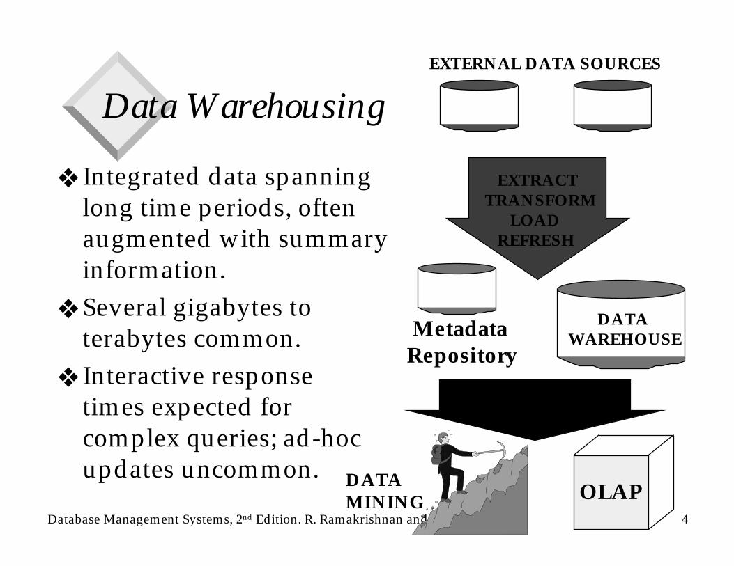
Data Warehousing

❖ Integrated data spanning long time periods, often augmented with summary information.

❖ Several gigabytes to terabytes common.

❖ Interactive response times expected for complex queries; ad-hoc updates uncommon.

EXTERNAL DATA SOURCES

EXTRACTTRANSFORM

LOADREFRESH

DATAWAREHOUSEMetadata

Repository

SUPPORTS

OLAPDATAMINING


Warehousing Issues❖ Semantic Integration: When getting data from

multiple sources, must eliminate mismatches, e.g., different currencies, schemas.

❖ Heterogeneous Sources: Must access data from a variety of source formats and repositories.– Replication capabilities can be exploited here.

❖ Load, Refresh, Purge: Must load data, periodically refresh it, and purge too-old data.

❖ Metadata Management: Must keep track of source, loading time, and other information for all data in the warehouse.


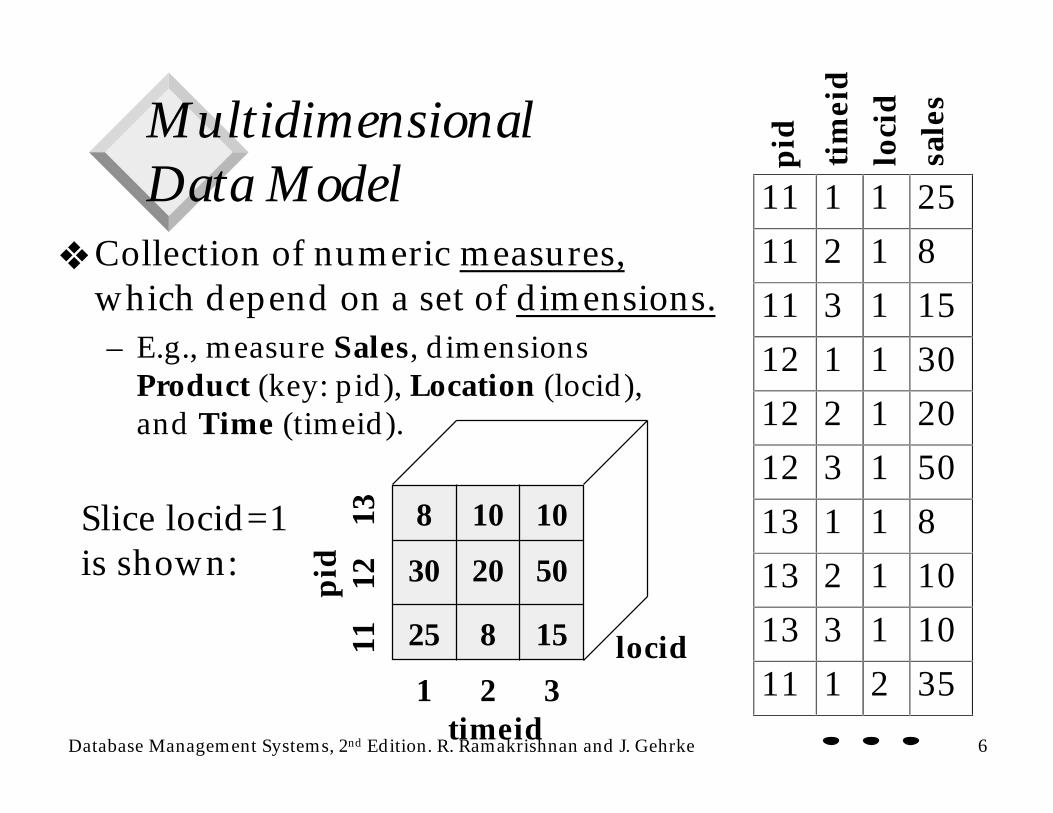
Multidimensional Data Model

❖ Collection of numeric measures,which depend on a set of dimensions.– E.g., measure Sales, dimensions

Product (key: pid), Location (locid), and Time (timeid).

8 10 10

30 20 50

25 8 15

1 2 3timeid

pid

11

12

13

11 1 1 25

11 2 1 8

11 3 1 15

12 1 1 30

12 2 1 20

12 3 1 50

13 1 1 8

13 2 1 10

13 3 1 10

11 1 2 35

pid tim

eid

loci

d

sale

s

locid

Slice locid=1is shown:


MOLAP vs ROLAP

❖ Multidimensional data can be stored physically in a (disk-resident, persistent) array; called MOLAP systems. Alternatively, can store as a relation; called ROLAP systems.

❖ The main relation, which relates dimensions to a measure, is called the fact table. Each dimension can have additional attributes and an associated dimension table.– E.g., Products(pid, pname, category, price)– Fact tables are much larger than dimensional tables.


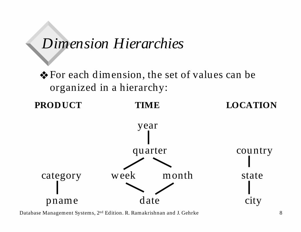
Dimension Hierarchies

❖ For each dimension, the set of values can be organized in a hierarchy:

PRODUCT TIME LOCATION

category week month state

pname date city

year

quarter country


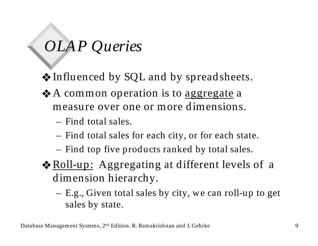
OLAP Queries

❖ Influenced by SQL and by spreadsheets.❖ A common operation is to aggregate a

measure over one or more dimensions.– Find total sales.– Find total sales for each city, or for each state.– Find top five products ranked by total sales.

❖ Roll-up: Aggregating at different levels of a dimension hierarchy. – E.g., Given total sales by city, we can roll-up to get

sales by state.


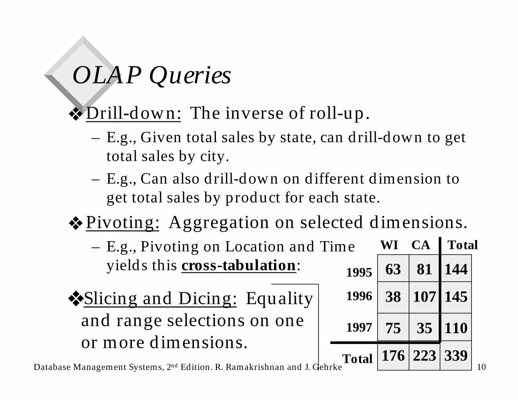
OLAP Queries❖ Drill-down: The inverse of roll-up.

– E.g., Given total sales by state, can drill-down to get total sales by city.

– E.g., Can also drill-down on different dimension to get total sales by product for each state.

❖ Pivoting: Aggregation on selected dimensions.– E.g., Pivoting on Location and Time

yields this cross-tabulation: 63 81 144

38 107 145

75 35 110

WI CA Total

1995

1996

1997

176 223 339Total

❖ Slicing and Dicing: Equalityand range selections on oneor more dimensions.


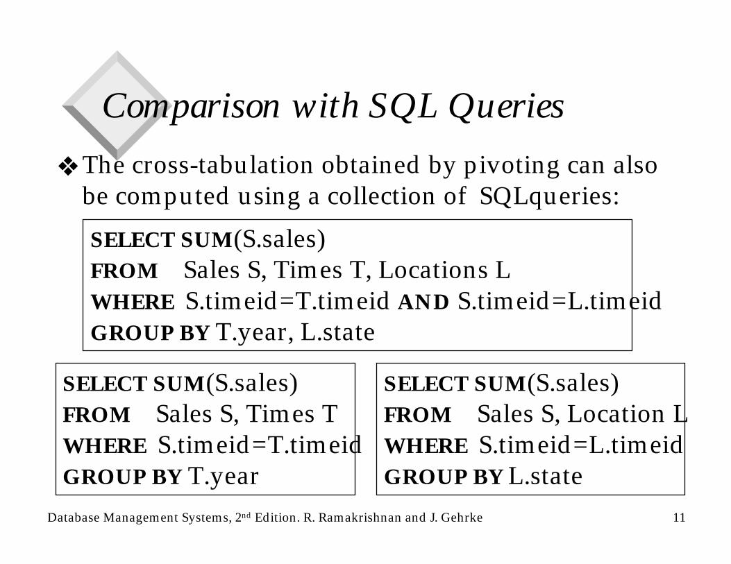
Comparison with SQL Queries

❖ The cross-tabulation obtained by pivoting can also be computed using a collection of SQLqueries:

SELECT SUM(S.sales)FROM Sales S, Times T, Locations LWHERE S.timeid=T.timeid AND S.timeid=L.timeidGROUP BY T.year, L.state

SELECT SUM(S.sales)FROM Sales S, Times TWHERE S.timeid=T.timeidGROUP BY T.year

SELECT SUM(S.sales)FROM Sales S, Location LWHERE S.timeid=L.timeidGROUP BY L.state


The CUBE Operator

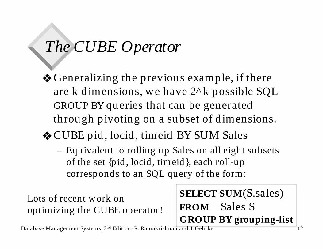
❖ Generalizing the previous example, if there are k dimensions, we have 2^k possible SQL GROUP BY queries that can be generated through pivoting on a subset of dimensions.

❖ CUBE pid, locid, timeid BY SUM Sales– Equivalent to rolling up Sales on all eight subsets

of the set {pid, locid, timeid}; each roll-up corresponds to an SQL query of the form:

SELECT SUM(S.sales)FROM Sales SGROUP BY grouping-list

Lots of recent work onoptimizing the CUBE operator!


Design Issues

❖ Fact table in BCNF; dimension tables not normalized.– Dimension tables are small; updates/inserts/deletes

are rare. So, anomalies less important than good query performance.

❖ This kind of schema is very common in OLAP applications, and is called a star schema; computing the join of all these relations is called

pricecategorypnamepid countrystatecitylocid

saleslocidtimeidpid

holiday_flag

weekdate

timeid

month

quarter

year

(Fact table)SALES

TIMES

PRODUCTS LOCATIONS


Implementation Issues❖ New indexing techniques: Bitmap indexes, Join

indexes, array representations, compression, precomputation of aggregations, etc.

❖ E.g., Bitmap index:

10100110

112 Joe M 3115 Ram M 5

119 Sue F 5

112 Woo M 4

00100000010000100010

sex custid name sex rating ratingBit-vector:1 bit for eachpossible value.Many queries canbe answered usingbit-vector ops!

MF


Join Indexes❖ Consider the join of Sales, Products, Times, and

Locations, possibly with additional selection conditions (e.g., country=“USA”).– A join index can be constructed to speed up such joins.

The index contains [s,p,t,l] if there are tuples (with sid) s in Sales, p in Products, t in Times and l in Locations that satisfy the join (and selection) conditions.

❖ Problem: Number of join indexes can grow rapidly.– A variant of the idea addresses this problem: For each

column with an additional selection (e.g., country), build an index with [c,s] in it if a dimension table tuple with value c in the selection column joins with a Sales tuple with sid s; if indexes are bitmaps, called


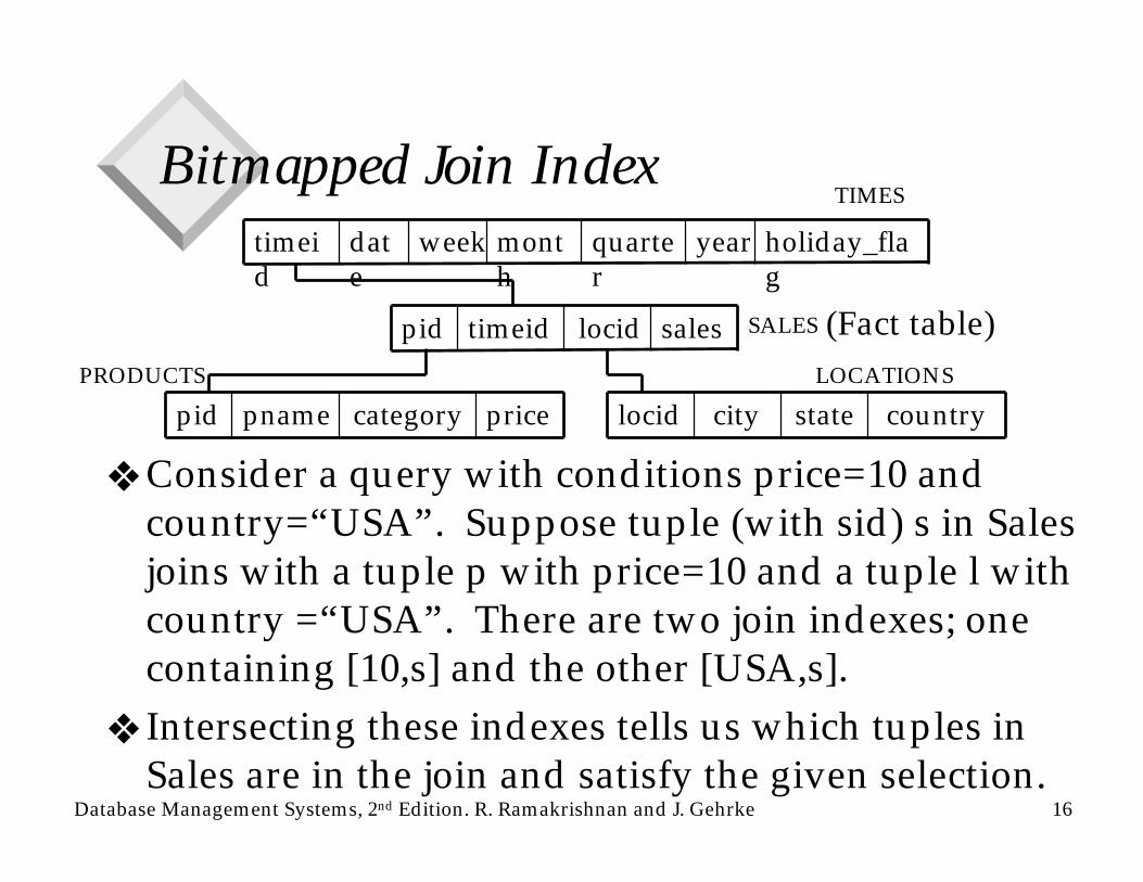
Bitmapped Join Index

❖ Consider a query with conditions price=10 and country=“USA”. Suppose tuple (with sid) s in Sales joins with a tuple p with price=10 and a tuple l with country =“USA”. There are two join indexes; one containing [10,s] and the other [USA,s].

❖ Intersecting these indexes tells us which tuples in Sales are in the join and satisfy the given selection.

pricecategorypnamepid countrystatecitylocid

saleslocidtimeidpid

holiday_flag

weekdate

timeid

month

quarter

year

(Fact table)SALES

TIMES

PRODUCTS LOCATIONS


Views and Decision Support

❖ OLAP queries are typically aggregate queries.– Precomputation is essential for interactive response

times.– The CUBE is in fact a collection of aggregate queries,

and precomputation is especially important: lots of work on what is best to precompute given a limited amount of space to store precomputed results.

❖ Warehouses can be thought of as a collection of asynchronously replicated tables and periodically maintained views.– Has renewed interest in view maintenance!


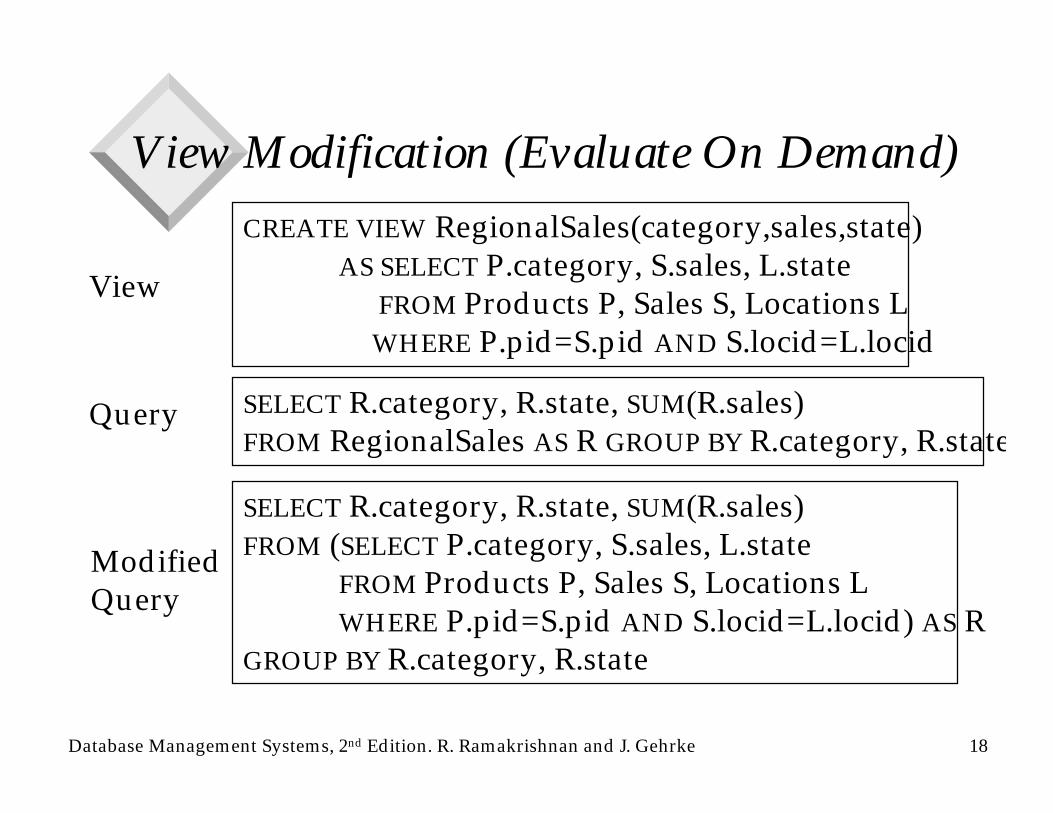
View Modification (Evaluate On Demand)CREATE VIEW RegionalSales(category,sales,state)

AS SELECT P.category, S.sales, L.stateFROM Products P, Sales S, Locations LWHERE P.pid=S.pid AND S.locid=L.locid

SELECT R.category, R.state, SUM(R.sales)FROM RegionalSales AS R GROUP BY R.category, R.state

SELECT R.category, R.state, SUM(R.sales)FROM (SELECT P.category, S.sales, L.state

FROM Products P, Sales S, Locations LWHERE P.pid=S.pid AND S.locid=L.locid) AS R

GROUP BY R.category, R.state

View

Query

ModifiedQuery


View Materialization (Precomputation)

❖ Suppose we precompute RegionalSales and store it with a clustered B+ tree index on [category,state,sales].– Then, previous query can be answered by an index-

only scan.SELECT R.state, SUM(R.sales)FROM RegionalSales RWHERE R.category=“Laptop”GROUP BY R.state

SELECT R.state, SUM(R.sales)FROM RegionalSales RWHERE R. state=“Wisconsin”GROUP BY R.category

Index on precomputed view is great!

Index is less useful (must scan entire leaf level).


Issues in View Materialization

❖ What views should we materialize, and what indexes should we build on the precomputed results?

❖ Given a query and a set of materialized views, can we use the materialized views to answer the query?

❖ How frequently should we refresh materialized views to make them consistent with the underlying tables? (And how can we do this incrementally?)


Interactive Queries: Beyond Materialization

❖ Top N Queries: If you want to find the 10 (or so) cheapest cars, it would be nice if the DB could avoid computing the costs of all cars before sorting to determine the 10 cheapest.– Idea: Guess at a cost c such that the 10 cheapest all

cost less than c, and that not too many more cost less. Then add the selection cost<c and evaluate the query.

◆ If the guess is right, great, we avoid computation for cars that cost more than c.

◆ If the guess is wrong, need to reset the selection and recompute the original query.


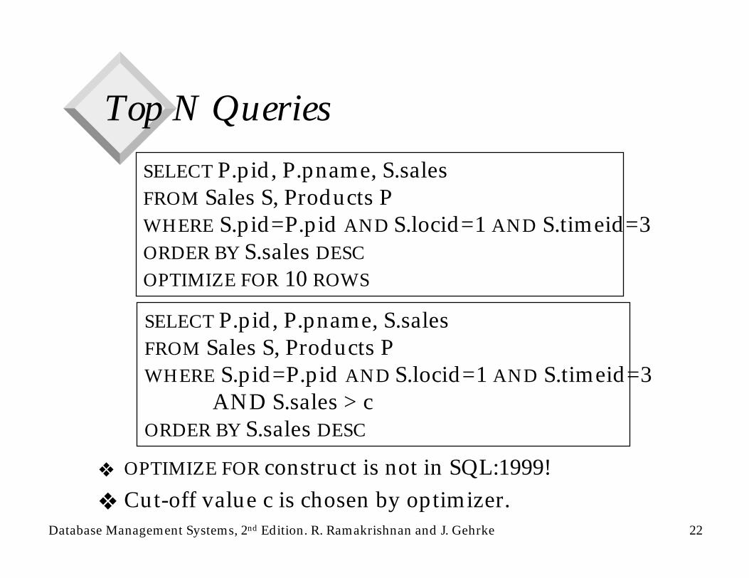
Top N Queries

SELECT P.pid, P.pname, S.salesFROM Sales S, Products PWHERE S.pid=P.pid AND S.locid=1 AND S.timeid=3ORDER BY S.sales DESCOPTIMIZE FOR 10 ROWS

❖ OPTIMIZE FOR construct is not in SQL:1999!❖ Cut-off value c is chosen by optimizer.

SELECT P.pid, P.pname, S.salesFROM Sales S, Products PWHERE S.pid=P.pid AND S.locid=1 AND S.timeid=3

AND S.sales > cORDER BY S.sales DESC


Interactive Queries: Beyond Materialization

❖ Online Aggregation: Consider an aggregate query, e.g., finding the average sales by state. Can we provide the user with some information before the exact average is computed for all states?– Can show the current “running average” for each

state as the computation proceeds.– Even better, if we use statistical techniques and

sample tuples to aggregate instead of simply scanning the aggregated table, we can provide bounds such as “the average for Wisconsin is 2000±102 with 95% probability.

◆ Should also use nonblocking algorithms!


Summary❖ Decision support is an emerging, rapidly

growing subarea of databases.❖ Involves the creation of large, consolidated

data repositories called data warehouses.❖ Warehouses exploited using sophisticated

analysis techniques: complex SQL queries and OLAP “multidimensional” queries (influenced by both SQL and spreadsheets).

❖ New techniques for database design, indexing, view maintenance, and interactive querying need to be supported.

Documents

Decision Support - uchile.clmnmonsal/BD/guias/OLAP-DataWH.pdf · Database Management Systems, 2nd Edition. R. Ramakrishnan and J. Gehrke 2 Introduction Increasingly, organizations