Embed Size (px)
Citation preview

DECISION SUPPORT SYSTEM FOR RESERVOIR OPERATION USING
ANALYTICAL MODELING RESULTS
BY
QIANKUN ZHAO
THESIS
Submitted in partial fulfillment of the requirements
for the degree of Master of Science in Civil Engineering
in the Graduate College of the
University of Illinois at Urbana-Champaign, 2017
Urbana, Illinois
Adviser:
Professor Ximing Cai

ii
ABSTRACT
This study applies an analytical approach to solving reservoir operation problems, in
particular, developing an algorithm to search for the optimal solution for a system of
reservoirs in parallel, establishing procedures to determine the effective forecast horizon,
and demonstrating the practical applications of the derived rules. Based on these, a decision
support system for reservoir operation is developed. More specifically, the analytical work
of this thesis includes two parts. In the first part, a multi-stage optimization model is set up
to derive the properties of optimal release decisions for a system of reservoirs in parallel
with a single demand site; following that an algorithm is developed using the analytical
results. In the second part, the properties of the optimal solution for a single water supply
reservoir under uncertain forecast are derived, and these properties are then used to develop
criteria and procedures to determine the effective forecast horizon, which can inform
reservoir managers in the actual use of inflow forecast. Finally, a prototype reservoir
operation decision support system is developed based on the analytical results. This system
is to illustrate the applications of analytically derived reservoir operation rules to guide
real-world reservoir operations. Through the system, users can use a graphical user
interface (GUI) to upload data, execute model, and visualize the results. As a conclusion,
being different from most existing studies using numerical models, this thesis shows the
capabilities of the analytical approaches in providing information for real-world reservoir
operation problems.

iii
ACKNOWLEDGEMENTS
I would like to express my appreciation to my advisor Professor Ximing Cai for his
patient and comprehensive guidance in completing and improving this thesis.
I would also like to thank my parents for their unreserved and continuous love and
support.

iv
TABLE OF CONTENTS
CHAPTER 1: INTRODUCTION ....................................................................................... 1
CHAPTER 2: GENERAL OPERATION RULES FOR SYSTEM OF RESERVOIRS IN
PARALLEL ........................................................................................................................ 6
CHAPTER 3: DETERMINING EFFECTIVE FORECAST HORIZON ......................... 40
CHAPTER 4: DECISION SUPPORT TOOL DEVELOPMENT .................................... 66
CHAPTER 5: CONCLUSIONS ....................................................................................... 72
REFERENCES ................................................................................................................. 74
APPENDIX A: DERIVATION ........................................................................................ 76
APPENDIX B: PROOF .................................................................................................... 79
APPENDIX C: DERIVATION ........................................................................................ 83
APPENDIX D: PROOF .................................................................................................... 85
APPENDIX E: PROOF .................................................................................................... 87
APPENDIX F: PROOF..................................................................................................... 89
APPENDIX G: PROOF .................................................................................................... 93

1
CHAPTER 1: INTRODUCTION
Reservoir operation is a fundamental issue for water resources planning and
management. Extensive efforts have been made to develop effective reservoir operation
policies including simulation and optimization models (Yeh, 1985; Wurbs,1993; Labadie,
2004). While the majority of the research has been with numerical approaches, such as
classic mathematical programming models, heuristic methods, and dynamic programming
techniques, which rely on computer programs to solve for solutions (e.g., Stedinger, Sule,
& Loucks, 1984; Wardlaw & Sharif, 1999), some studies used analytical approach to derive
general rules and insights for reservoir operation rules (e.g., Lund & Guzman,1999; You &
Cai, 2008a, 2008b). The most remarkable reservoir operation rule obtained from analytical
derivations is probably the NYC rules (Clark, 1950) for parallel reservoir system operation,
which minimizes the total expected spills from all the reservoirs in the system, and the
NYC rules have been used for a long time.
Instead of minimizing spills or maximizing total available water though a numerical
model, Draper & Lund (2004) introduced concave economic benefit functions for both the
release and the carry-over storage, and set up a general economic principle to obtain the
optimal operation policy to maximize the total economic benefit of the current release and
the carry-over storage for the future. You & Cai (2008a) extended this work by explicitly
including uncertainty in future inflow and developed hedging policies with a conceptual
two-stage model. Following that, the economic views and analytical optimization
approaches are further applied to addressing the various issues of reservoir operation. Zhao
et al. (2011) formulated a two-stage model to maximize the total benefit of the releases
over two stages, an optimal solution was solved using Karush–Kuhn–Tucker KKT
conditions, and an algorithm was developed based on the analytical results to solve the

2
problem numerically. Following Zhao et al. (2011), Xu et al. (2014) extended the two-stage
model to a multi-stage model with explicitly incorporated uncertain inflow forecast, and
developed a numerical algorithm based on the optimality conditions. Instead of
maximizing the total economic benefits, Shiau (2011) derived a two-point hedging rule for
a single reservoir operation by minimizing a loss function in terms of the deviations of the
current release and carry-over storage from the predetermined targets. Zeng et al. (2015)
extended the analysis from a single reservoir to a system of multi-reservoirs in parallel, and
derived optimal operation policies by setting the loss function in terms of the deviations of
both the individual reservoir carry-over storages and the system-level release decisions
from the predetermined targets. Studies are also conducted for flood management purposes,
including studies on hedging between post-flood water conservation and flood risk (e.g.,
Ding et al., 2015, 2017; Wan et al., 2016) and studies on pre-releasing to allocate storage
capacity between floods at current stage and future stages (e.g., Zhao et al., 2014; Hui &
Lund, 2015).
This work follows the analytical frame work by Draper & Lund (2004), You & Cai
(2008a) to explore more capabilities of the analytical approaches in providing solutions for
reservoir operation related issues, e.g., algorithms development, theory proof, tool design,
etc.
Due to the system complexity, deriving operation policies for a system of reservoirs
in parallel is challenging (Oliverira and Loucks, 1997; Labadie, 2004). Most research relies
on numerical methods, especially, heuristic methods, to explore operation policies for
multi-reservoir systems (e.g., Chang & Change, 2009; Jalali et al., 2007; Wardlaw & Sharif,
1999). On the one hand, though reasonable results might be obtained from these numerical
methods, the general properties of optimal operation policies for parallel reservoir systems
can hardly be represented, explicitly. On the other hand, many of these numerical methods,
especially the widely used stochastic dynamic programming approach, suffer from

3
computational burden induced by the high dimensionality of the problems (Castelletti et
al., 2010; Jairaj & Vedula, 2003). As compared to the most widely-used numerical
approaches, analytical approaches, though limited by assumptions and simplifications,
provide optimal solutions for a system of reservoirs in parallel with less computational
requirements and more general insights. Zeng et al. (2015) derived the optimal operation
policy for a multi-reservoir system in parallel with a joint demand site by minimizing a
loss function in terms of the deviation of carry-over storage of the individual reservoirs and
the system-level release decisions from the predetermined targets. However, in Zeng et al.
(2015), the coordination of the operation of reservoirs in the system can only be partially
revealed as the coordination also depends on the predetermined targets. To explore general
insights for coordinating the operation of a system of reservoirs in parallel and develop
computationally efficient algorithms, this thesis will analytically derive the operation rules
for such a system with a single demand site by maximizing a benefit function evaluated at
the demand site through a multistage optimization model; following that, an algorithm will
be developed to solve the optimization problem. Being different from Zhao et al. (2011)
and Xu et al. (2014), who designed algorithms for single reservoir operation by recursively
searching the solution based on the optimality conditions, in this study, the algorithm will
be designed based on the insights obtained from the analytical results, and will solve the
problem efficiently despite for the complexity with the high-dimensional system.
The concept of hedging in reservoir operation was first provided by Bower et al.
(1962), and has been widely explored (Neelakantan & Sasireka, 2015). By hedging rules,
water will be allocated between current and future stages. Instead of satisfying the water
demand at current stage with the first priority, as the standard operation policy (SOP)
proposes, hedging rules allow reducing release at the current stage and reserve some
amount of water for the future to mitigate possible water stress in the future. Inflow forecast,
thus, is of great importance to achieve better hedging performance. It has been

4
demonstrated that inflow forecast is important for making reservoir operation decisions
(Zhao et al., 2011), while imperfect forecast might significantly reduce the usefulness of
the forecast information (Mishalani and Palmer, 1988). To address the issues of
determining an appropriate forecast horizon for reservoir operation decision making, You
and Cai (2008c) developed a theoretical relationship for determining the forecast horizon
using dimensional analysis. The forecast horizon is defined as the length of the forecast
beyond which the inflow will no longer affect the release decision at the current stage (e.g.,
in decision horizon.) Zhao et al. (2012) conducted numerical experiments with imperfect
forecast and proposed the concept of effective forecast horizon (EFH) with a certain level
of uncertainty, which provides maximum information to support reservoir operation
decisions. Though promising concepts are provided by You and Cai (2008c) and Zhao et
al. (2012), procedures are still needed to determine the EFH. In this thesis, a relationship
between the forecast uncertainty and the decision uncertainty is derived analytically, which
is further applied to providing criteria and procedures for determining the EFH.
Though there is growing amount of research applying analytical approaches to
addressing reservoir operation issues, there exists rarely any decision support tool based
on these results for real world reservoir operations. Most existing reservoir operation
decision support tools rely on numerical methods for simulation or optimization (e.g.,
Koutsoyiannis et al., 2002), and a large portion of them are case-specific (e.g.,
Chandramouli & Deka, 2005). Thus, to provide a new approach and to show the potential
of using analytically derived results, a prototype reservoir operation decision support
system is developed based on the analytical results obtained from this and other studies.
The rest of thesis will be organized as follows. In the Chapter 2, a multi-stage
optimization model is set up to discuss the properties of the optimal release decision for a
system of multi-reservoir in parallel and an algorithm is further developed based on the
analytical results; In the Chapter 3, a multi-stage reservoir operation model is set up for a

5
single reservoir with a single demand site; following that, criteria and procedures for
determining the EFH are developed. In Chapter 4, a prototype reservoir operation decision
support system is described and demonstrated. Finally, conclusions are provided in Chapter
5.

6
CHAPTER 2: GENERAL OPERATION
RULES FOR SYSTEM OF RESERVOIRS
IN PARALLEL
2.1 Background
In Zeng et al. (2015), hedging rules for a system of reservoirs in parallel has been
discussed with a two-stage model given a storage target for each reservoir and a system
level release target, and a two-point hedging curve is derived. However, the work can only
partially represent the actual cooperation between reservoirs in parallel since part of the
actual cooperation may be reflected by the given storage and release targets. Following
Zeng et al. (2015), we derive general rules for the operation of a system of reservoirs in
parallel using a multi-stage model with the utility function evaluated at a single demand
site, which attempts to include more real-world corporation rules among parallel reservoirs
associated with a water supply system. Cooperation between parallel reservoirs is
investigated, and an algorithm is developed based on the analytical results. The results from
this section could reveal some insights for parallel reservoir operation and can also be used
to provide optimal operation decisions for real-world operation of a system of reservoirs in
parallel.
2.2 Model Formulation and Discussion
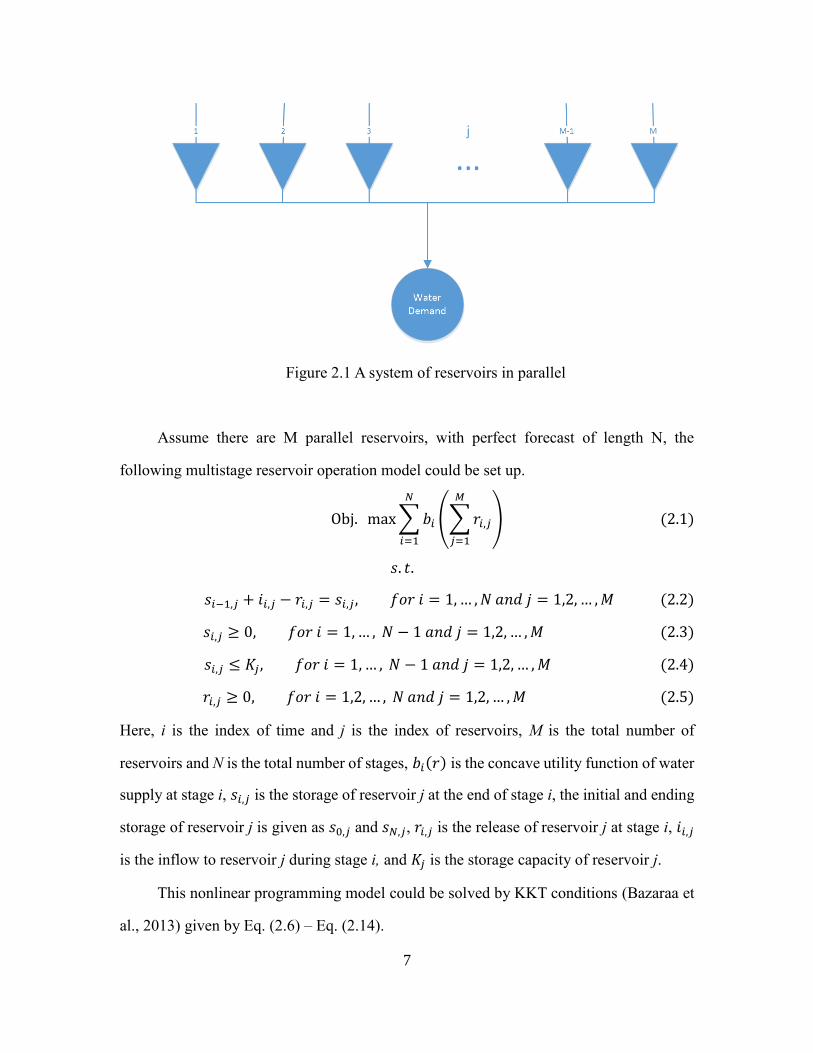
A parallel reservoir system with M parallel reservoirs supplying water for a single
demand site is investigated, the water supply system is illustrated in Figure 2.1.
7
Figure 2.1 A system of reservoirs in parallel
Assume there are M parallel reservoirs, with perfect forecast of length N, the
following multistage reservoir operation model could be set up.
Obj. max∑𝑏𝑖 (∑𝑟𝑖,𝑗
𝑀
𝑗=1
)
𝑁
𝑖=1
(2.1)
𝑠. 𝑡.
𝑠𝑖−1,𝑗 + 𝑖𝑖,𝑗 − 𝑟𝑖,𝑗 = 𝑠𝑖,𝑗, 𝑓𝑜𝑟 𝑖 = 1,… ,𝑁 𝑎𝑛𝑑 𝑗 = 1,2, … ,𝑀 (2.2)
𝑠𝑖,𝑗 ≥ 0, 𝑓𝑜𝑟 𝑖 = 1,… , 𝑁 − 1 𝑎𝑛𝑑 𝑗 = 1,2, … ,𝑀 (2.3)
𝑠𝑖,𝑗 ≤ 𝐾𝑗, 𝑓𝑜𝑟 𝑖 = 1,… , 𝑁 − 1 𝑎𝑛𝑑 𝑗 = 1,2, … ,𝑀 (2.4)
𝑟𝑖,𝑗 ≥ 0, 𝑓𝑜𝑟 𝑖 = 1,2, … , 𝑁 𝑎𝑛𝑑 𝑗 = 1,2, … ,𝑀 (2.5)
Here, i is the index of time and j is the index of reservoirs, M is the total number of
reservoirs and N is the total number of stages, 𝑏𝑖(𝑟) is the concave utility function of water
supply at stage i, 𝑠𝑖,𝑗 is the storage of reservoir j at the end of stage i, the initial and ending
storage of reservoir j is given as 𝑠0,𝑗 and 𝑠𝑁,𝑗, 𝑟𝑖,𝑗 is the release of reservoir j at stage i, 𝑖𝑖,𝑗
is the inflow to reservoir j during stage i, and 𝐾𝑗 is the storage capacity of reservoir j.
This nonlinear programming model could be solved by KKT conditions (Bazaraa et
al., 2013) given by Eq. (2.6) – Eq. (2.14).

8
−∇∑𝑏𝑖 (∑𝑟𝑖,𝑗
𝑀
𝑗=1
)
𝑁
𝑖=1
+ ∇∑∑𝜆𝑏,𝑖,𝑗(𝑠𝑖,𝑗 − 𝑠𝑖−1,𝑗 − 𝑖𝑖,𝑗 + 𝑟𝑖,𝑗)
𝑀
𝑗=1
𝑁
𝑖=1
+ ∇∑∑𝜆𝑒,𝑖,𝑗(−𝑠𝑖,𝑗)
𝑀
𝑗=1
𝑁−1
𝑖=1
+ ∇∑∑𝜆𝑓,𝑖,𝑗(𝑠𝑖,𝑗 − 𝐾𝑗)
𝑀
𝑗=1
𝑁−1
𝑖=1
+ ∇∑∑𝜆𝑟,𝑖,𝑗(−𝑟𝑖,𝑗)
𝑀
𝑗=1
𝑁
𝑖=1
,
𝑓𝑜𝑟 𝑖 = 1, … , 𝑁 − 1 𝑎𝑛𝑑 𝑗 = 1,2, … ,𝑀 (2.6)
−𝑠𝑖,𝑗 ≤ 0, 𝑓𝑜𝑟 𝑖 = 1,… ,𝑁 − 1 𝑎𝑛𝑑 𝑗 = 1,2, … ,𝑀 (2.7)
𝑠𝑖,𝑗 ≤ 𝐾𝑖, 𝑓𝑜𝑟 𝑖 = 1,… ,𝑁 − 1 𝑎𝑛𝑑 𝑗 = 1,2, … ,𝑀 (2.8)
𝜆𝑒,𝑖,𝑗𝑠𝑖,𝑗 = 0, 𝑓𝑜𝑟 𝑖 = 1,… ,𝑁 − 1 𝑎𝑛𝑑 𝑗 = 1,2, … ,𝑀 (2.9)
𝜆𝑓,𝑖,𝑗(𝑠𝑖,𝑗 − 𝐾𝑖) = 0, 𝑓𝑜𝑟 𝑖 = 1,… ,𝑁 − 1 𝑎𝑛𝑑 𝑗 = 1,2, … ,𝑀 (2.10)
𝜆𝑟,𝑖,𝑗𝑟𝑖,𝑗 = 0, 𝑓𝑜𝑟 𝑖 = 1,… ,𝑁 𝑎𝑛𝑑 𝑗 = 1,2, … ,𝑀 (2.11)
𝜆𝑒,𝑖,𝑗 ≥ 0, 𝑓𝑜𝑟 𝑖 = 1, … , 𝑁 − 1 𝑎𝑛𝑑 𝑗 = 1,2, … ,𝑀 (2.12)
𝜆𝑓,𝑖,𝑗 ≥ 0, 𝑓𝑜𝑟 𝑖 = 1, … , 𝑁 − 1 𝑎𝑛𝑑 𝑗 = 1,2, … ,𝑀 (2.13)
𝜆𝑟,𝑖,𝑗 ≥ 0 𝑓𝑜𝑟 𝑖 = 1,2, … ,𝑁 𝑎𝑛𝑑 𝑗 = 1,2, … ,𝑀 (2.14)
Here, 𝜆𝑏,𝑖,𝑗 is the shadow price for the mass balance constrain, Eq. (2.2), of reservoir j at
stage i, 𝜆𝑒,𝑖,𝑗 is the shadow price for non-negative storage constraints, Eq. (2.3), of reservoir
j at the end of stage i, 𝜆𝑓,𝑖,𝑗 is the shadow price for storage capacity constraints, Eq. (2.4),
of reservoir j at the end of stage i, and 𝜆𝑟,𝑖,𝑗 is the shadow price for non-negative release
constraints, Eq. (2.5), of reservoir j on stage i.
To simplify representation, let 𝑟𝑖 represent the sum of release at stage i from all
reservoirs.
𝑟𝑖 =∑𝑟𝑖,𝑗
𝑀
𝑗=1
(2.15)
Note, at the same stage, the following formula should be satisfied according to the property
of derivatives as shown in Eq. (2.16).
𝜕𝑏𝑖(∑ 𝑟𝑖,𝑗𝑀𝑗=1 )
𝜕𝑟𝑖=𝜕𝑏𝑖(∑ 𝑟𝑖,𝑗
𝑀𝑗=1 )
𝜕𝑟𝑖,𝑗= 𝑏𝑖
′ (∑𝑟𝑖,𝑗
𝑀
𝑗=1
) (2.16)

9
Physically, this means that, at stage i, the marginal utility (MU) of release from each
reservoir is identical to each other.
By KKT conditions, following relationship could be obtained (See Appendix A).
𝑏𝑖+1′ (∑𝑟𝑖+1,𝑗
𝑀
𝑗=1
) + 𝜆𝑒,𝑖,𝑗 + 𝜆𝑟,𝑖+1,𝑗 = 𝑏𝑖′ (∑𝑟𝑖,𝑗
𝑀
𝑗=1
) + 𝜆𝑓,𝑖,𝑗 + 𝜆𝑟,𝑖,𝑗 (2.17)
Three different scenarios are discussed based on the relationships between the
marginal utilities (MU) at two consecutive stages (as shown in Figure 2.2).
Marginal Utility at Stage i+1
Mar
gin
al U
tili
ty a
t S
tag
e i
Scenario 2
Scenario 1
Figure 2.2 Illustration of three different scenarios
Scenario 1:
If for two consecutive stages (stage i and i+1), we have the following relationship,
i.e., the MU level becomes higher at next stage,
𝑏𝑖+1′ (∑𝑟𝑖+1,𝑗
𝑀
𝑗=1
) > 𝑏𝑖′ (∑𝑟𝑖,𝑗
𝑀
𝑗=1
) (2.18)
then,

10
𝜆𝑟,𝑖,𝑗 + 𝜆𝑓,𝑖,𝑗 = 𝑃 + 𝜆𝑟,𝑖+1,𝑗 + 𝜆𝑒,𝑖,𝑗 , 𝑓𝑜𝑟 𝑗 = 1,2, … ,𝑀 (2.19)
where P is a positive number as defined below:
𝑃 = 𝑏𝑖+1′ (∑𝑟𝑖+1,𝑗
𝑀
𝑗=1
) − 𝑏𝑖′ (∑𝑟𝑖,𝑗
𝑀
𝑗=1
) > 0 (2.20)
All reservoirs must satisfy the relationship shown in Eq. (2.19). Any of the reservoirs
can have one of the following three cases:
(1) If 𝜆𝑒,𝑖,𝑗=0 (i.e., reservoir j is usually not empty at the end of stage i) and 𝜆𝑓,𝑖,𝑗 = 0 (i.e.,
reservoir j is usually not full at the end of stage i),
𝜆𝑟,𝑖,𝑗 = 𝑃 + 𝜆𝑟,𝑖+1,𝑗 (2.21)
Therefore,
𝜆𝑟,𝑖,𝑗 > 0 (2.22)
This means there is no release from the reservoir at stage i (by Eq. (2.22)). This shows that
the following three conditions might match together as part of the optimization conditions:
the MU level increases from stage i to stage i+1 (Eq. (2.18)), the storage is at any level1 at
the end of stage i, and the reservoir does not release at stage i (Figure 2.3(a)). Under this
case, as the MU increases, the reservoir tends to save more water to the future stage with
higher MU, and as a result, all inflow at stage i is kept in the reservoir. This indicates that
the reservoir capacity is not the controlling factor and the inflow condition limits the ability
for the reservoir to save more water to the future.
(2) If 𝜆𝑒,𝑖,𝑗>0 (i.e., reservoir j is empty at stage at the end stage i), and we must have 𝜆𝑓,𝑖,𝑗 =
0 (i.e., the reservoir j is not full at the end of stage i), then:
𝜆𝑟,𝑖,𝑗 = 𝑃 + 𝜆𝑒,𝑖,𝑗 + 𝜆𝑟,𝑖+1,𝑗 (2.23)
Therefore,
𝜆𝑟,𝑖,𝑗 > 0 (2.24)
1 Under extreme cases, the reservoir can be full but no benefit associated with keeping more water in the reservoir or
empty but no benefit associated with releasing more water from the reservoir.

11
This means there is no release from the reservoir at stage i (Eq. (2.24)). This shows that the
following three conditions might match together as part of the optimization conditions: the
MU level increases from stage i to stage i+1, the reservoir is empty at the end of stage i
and the reservoir does not release at stage i (Figure 2.3(b)). This is only possible if there is
no inflow during stage i and the initial storage of stage i is zero (otherwise there should be
some water saved at the end of i). Under such conditions, the reservoir is dry and has no
release. Even though the MU increases, the inflow condition limits the ability for the
reservoir to save water to the future stages with higher MU.
(3) If 𝜆𝑒,𝑖,𝑗 =0 (i.e., reservoir j is not empty at the end of stage i), and 𝜆𝑓,𝑖,𝑗 > 0 (i.e.,
reservoir j at stage is full at the end of stage i),
𝜆𝑟,𝑖,𝑗 + 𝜆𝑓,𝑖,𝑗 = 𝑃 + 𝜆𝑟,𝑖+1,𝑗 (2.25)
Thus, either 𝜆𝑟,𝑖,𝑗 > 0 or 𝜆𝑟,𝑖,𝑗 = 0 is possible, and thus, the reservoir can release or not
release during stage i. This shows that the following two conditions might match together
as part of the optimization conditions: the MU level increases from stage i to stage i+1, the
reservoir becomes full at the end of stage i (Figure 2.3(c)). Under this case, as the MU
increases, the reservoir tends to save more water to the future stage with higher MU, and
as a result, the reservoir is full at the end of stage i. This indicates that the reservoir capacity
limits the ability for the reservoir to save more water to the future.
As a summary, under Scenario 1, when the MU level increases from stage i to i+1,
one of the following situations must occur for any reservoir in the system under an optimal
solution:
a. Having a full storage at the end of stage i (corresponds to case (3) with limited capacity);
b. Having no release during stage i and save water to stage i+1 (corresponds to case (1) and
(2) with limited inflow).

12
Stage i Stage i+1
Rele
ase
Legend
MU
Feasible ReleaseMU of Released Water
𝜆𝑟 ,𝑖,𝑗 𝜆𝑟 ,𝑖+1,𝑗 ≥ 0
Any Storage
(a) Storage capacity and non-negative storage constraint unbinding
Stage i Stage i+1
Rele
ase
MU
𝜆𝑟 ,𝑖,𝑗 𝜆𝑟 ,𝑖+1,𝑗 ≥ 0
Empty Storage
LegendFeasible ReleaseMU of Released Water
𝜆𝑒 ,𝑖,𝑗 > 0
(b) Non-negative storage constraint binding
Stage i Stage i+1
Rele
ase
MU
𝜆𝑟 ,𝑖,𝑗 ≥ 0
Full Storage
𝜆𝑟 ,𝑖+1,𝑗 ≥ 0
LegendFeasible ReleaseMU of Released Water
𝜆𝑓 ,𝑖,𝑗 > 0
(c) Storage capacity constraint binding
Figure 2.3 Different cases with increasing MU

13
Scenario 2:
If for two consecutive stages (stage i and i+1), we have the following relationship,
i.e., the MU becomes lower on next stage (i+1),
𝑏𝑖+1′ (∑𝑟𝑖+1,𝑗
𝑀
𝑗=1
) < 𝑏𝑖′ (∑𝑟𝑖,𝑗
𝑀
𝑗=1
) (2.26)
then,
𝜆𝑟,𝑖,𝑗 + 𝜆𝑓,𝑖,𝑗 + 𝑃 = 𝜆𝑒,𝑖,𝑗 + 𝜆𝑟,𝑖+1,𝑗 , 𝑓𝑜𝑟 𝑗 = 1,2, … ,𝑀 (2.27)
where P is a positive number with the following definition:
𝑃 = 𝑏𝑖′ (∑𝑟𝑖,𝑗
𝑀
𝑗=1
) − 𝑏𝑖+1′ (∑𝑟𝑖+1,𝑗
𝑀
𝑗=1
) > 0 (2.28)
All reservoirs must satisfy the relationship shown in Eq. (2.27). Any of the reservoirs can
have one of the following three situations:
(1) If 𝜆𝑒,𝑖,𝑗=0 (i.e., reservoir j is usually not empty at the end of stage i) and 𝜆𝑓,𝑖,𝑗 = 0 (i.e.,
reservoir j is usually not full at the end of stage i),
𝜆𝑟,𝑖,𝑗 + 𝑃 = 𝜆𝑟,𝑖+1,𝑗 (2.29)
Therefore,
𝜆𝑟,𝑖+1,𝑗 > 0 (2.30)
This means there is no release from the reservoir at stage i+1. This shows that the following
three conditions might match together as part of the optimization conditions: the MU
decreases from stage i to stage i+1, the storage could be at any level at the end of stage i2
and the reservoir does not release at stage i+1 (Figure 2.4(a)). Under this case, as the MU
is decreasing, the reservoir tends to use more water at the current stage with higher MU.
However, the reservoir may not be empty at the end of stage i. One possible explanation
is that, if the reservoir is large enough, it can store part of the inflow from the current stage
2 Under some special cases, it is possible for the reservoir to be full but no benefit associated with keeping more water
in the reservoir or empty but no benefit associated with releasing more water from the reservoir.

14
and all inflows in the coming stages with lower MU than that of the current stage, for a
longer time to a future stage when the MU level is even higher than the current MU. This
indicates that the situation that a relative large capacity and limited inflow make it possible
for the reservoirs not to be empty and still store some water for the future when the MU
decreases.
(2) If 𝜆𝑒,𝑖,𝑗>0 (i.e., reservoir j is empty at stage at the end of stage i), and we must have
𝜆𝑓,𝑖,𝑗 = 0 (i.e., the reservoir j is not full at the end of stage i), then:
𝜆𝑟,𝑖,𝑗 + 𝑃 = 𝜆𝑟,𝑖+1,𝑗 + 𝜆𝑒,𝑖,𝑗 (2.31)
Thus, the reservoir can release or not release on both stage i and stage i+1. This shows that
the following two conditions might match together as part of the optimization conditions:
the MU decreases from stage i to stage i+1 and the reservoir becomes empty at the end of
stage i, (Figure 2.4(b)). Under this situation, as the MU is decreasing, the reservoir tends
to use more water at the current stage; as a result, the reservoir becomes empty at the end
of stage i. From another point of view, the reservoir is making space to store inflows during
the coming stages with lower MU. Thus, the storage capacity is the actual limiting factor
in this case.
(3) If 𝜆𝑒,𝑖,𝑗 =0 (i.e., reservoir j is not empty at the end of stage i), and 𝜆𝑓,𝑖,𝑗 > 0 (i.e.,
reservoir j at stage is full at the end of stage i),
𝜆𝑟,𝑖,𝑗 + 𝑃 + 𝜆𝑓,𝑖,𝑗 = 𝜆𝑟,𝑖+1,𝑗 (2.32)
Therefore,
𝜆𝑟,𝑖+1,𝑗 > 0 (2.33)
This means there is no release from the reservoir at stage i+1. Thus, the following three
conditions might match together as part of the optimization conditions: the MU level
decreases from stage i to stage i+1, the reservoir becomes full at the end of stage i, and the
reservoir has no release at stage i+1 (Figure 2.4 (c)). This is only possible if there is no
inflow during stage i+1 and the ending storage of stage i+1 is full too. Under such

15
conditions, the reservoir is full and has no release. Similar as Case (1) under Scenario 2,
the limited inflow makes it possible for reservoirs not to become empty when the MU
decreases.
As a summary, under Scenario 2, when the MU level decreases from stage i to i+1,
one of the following situations must occur for any reservoir in the system with the optimal
solution:
a. having an empty storage at the end of stage i (corresponds to case (2) with a limited
capacity);
b. having no release at stage i+1, i.e., having enough capacity to store all inflow during the
coming stages with low MU (corresponds to case (1) & (3) with limited inflow).
Stage i Stage i+1
Rele
ase
MU
𝜆𝑟 ,𝑖+1,𝑗 > 0
𝜆𝑟 ,𝑖,𝑗 ≥ 0
Any Storage
LegendFeasible ReleaseMU of Released Water
(a) Storage capacity and non-negative storage constraints unbinding
Stage i Stage i+1
Rele
ase
MU
𝜆𝑟 ,𝑖+1,𝑗 ≥ 0
Empty Storage
LegendFeasible ReleaseMU of Released Water
𝜆𝑒 ,𝑖,𝑗 > 0
(b) Non-negative storage constraint binding
Figure 2.4 Different cases with decreasing MU

16
Figure 2.4 (cont.)
Stage i Stage i+1
Rele
ase
MU
𝜆𝑟 ,𝑖+1,𝑗 > 0 𝜆𝑟 ,𝑖,𝑗 ≥ 0
Full Storage
LegendFeasible ReleaseMU of Released Water
𝜆𝑓 ,𝑖,𝑗 > 0
(c) Storage capacity constraint binding
Scenario 3:
In this scenario, storage and release conditions for two consecutive stages with
identical MU are considered,
𝑏𝑖+1′ (∑𝑟𝑖+1,𝑗
𝑀
𝑗=1
) = 𝑏𝑖′ (∑𝑟𝑖,𝑗
𝑀
𝑗=1
) (2.34)
The following relationship is achieved between these two stages.
𝜆𝑟,𝑖,𝑗 + 𝜆𝑓,𝑖,𝑗 = 𝜆𝑒,𝑖,𝑗 + 𝜆𝑟,𝑖+1,𝑗 , 𝑓𝑜𝑟 𝑗 = 1,2, … ,𝑀 (2.35)
All reservoirs must satisfy the relationship shown in Eq. (2.35). Any of the reservoirs can
have one of the following three situations:
(1) If 𝜆𝑒,𝑖,𝑗=0 (i.e., reservoir j is usually not empty at the end of stage i) and 𝜆𝑓,𝑖,𝑗 = 0 (i.e.,
reservoir j is usually not full at the end of stage i),
𝜆𝑟,𝑖,𝑗 = 𝜆𝑟,𝑖+1,𝑗 (2.36)
If 𝜆𝑟,𝑖,𝑗 > 0 , then 𝜆𝑟,𝑖+1,𝑗 > 0 , this means that for these two consecutive stages, the
reservoir keeps not releasing (Figure 2.5(b)), otherwise, if 𝜆𝑟,𝑖,𝑗 = 0, then 𝜆𝑟,𝑖+1,𝑗 = 0, this
means the reservoir should release or possibly not release. (Figure 2.5(a)). This shows that,
for any reservoir in the system, the following three conditions might match together as part

17
of the optimization conditions: the MU does not change from stage i to stage i+1, and the
storage is usually neither full nor empty3 and the operation for the reservoir keeps the same
at stage i and stage i+1, i.e., if the reservoir releases water during stage i, it can release
water during stage i+1, and vice versa.
(2) If 𝜆𝑒,𝑖,𝑗>0 (i.e., reservoir j is empty at stage at the end of stage i), and we must have
𝜆𝑓,𝑖,𝑗 = 0 (i.e., the reservoir j is not full at the end of stage i), then:
𝜆𝑟,𝑖,𝑗 = 𝜆𝑟,𝑖+1,𝑗 + 𝜆𝑒,𝑖,𝑗 (2.37)
Therefore,
𝜆𝑟,𝑖,𝑗 > 0 (2.38)
This means that this reservoir can become empty if it does not release at stage i (Figure
2.5(c)). This shows that the following three conditions might match together as part of the
optimization conditions: the MU does not change from stage i to stage i+1, the reservoir is
empty at the end of stage i, and there is no release at stage i. This is only possible if there
is no inflow during stage i and the initial storage of stage i is zero. Under such conditions,
the reservoir is dry and does not release.
(3) If 𝜆𝑒,𝑖,𝑗 =0 (i.e., reservoir j is not empty at the end of stage i), and 𝜆𝑓,𝑖,𝑗 > 0 (i.e.,
reservoir j at stage is full at the end of stage i),
𝜆𝑟,𝑖,𝑗 + 𝜆𝑓,𝑖,𝑗 = 𝜆𝑟,𝑖+1,𝑗 (2.39)
Therefore,
𝜆𝑟,𝑖+1,𝑗 > 0 (2.40)
which means that this reservoir can be full when it has no release at the next stage (Figure
2.5(d)). This means, for any reservoir in the system, the following three conditions might
match together as part of the optimization conditions: the MU does not change from stage
i to stage i+1, the reservoir is full at the end of stage i, and there is no release at stage i+1.
3 Under the following special cases the reservoir is possibly full or empty: the reservoir is full but there is no benefit
associated with keeping more water in the reservoir or empty but there is no benefit associated with releasing more
water from the reservoir.

18
This is only possible if there is no inflow during stage i+1 and the ending storage of stage
i+1 is full. Under such conditions, the reservoir is full and does not release.
As a summary, with identical MU between stage i and i+1, one of the following
situations must occur for any reservoir in the system with the optimal solution:
a. the reservoir is usually neither full nor empty at the end of stage i, and it releases at
neither stage;
b. the reservoir is usually neither full nor empty at the end of stage i, and the reservoir can
release at both stages.
c. There is no inflow at stage i and the reservoir keeps dry before stage i.
d. there is no inflow at stage i+1 and the reservoir remains full after stage i.
Stage i Stage i+1
Rele
ase
MU
𝜆𝑟𝑒𝑙𝑒𝑎𝑠𝑒 ,𝑖,𝑗 = 𝜆𝑟𝑒𝑙𝑒𝑎𝑠𝑒 ,𝑖+1,𝑗 = 0
Any Storage
LegendFeasible ReleaseMU of Released Water
𝜆𝑟 ,𝑖,𝑗 𝜆𝑟 ,𝑖+1,𝑗
(a) Storage capacity, non-negative storage and non-negative release constraints
unbinding
Figure 2.5 Different cases with identical MU

19
Figure 2.5 (cont.)
Stage i Stage i+1
Rele
ase
MU
Zero Release
𝜆𝑟𝑒𝑙𝑒𝑎𝑠𝑒 ,𝑖,𝑗 = 𝜆𝑟𝑒𝑙𝑒𝑎𝑠𝑒 ,𝑖+1,𝑗 > 0
Any Storage
LegendFeasible ReleaseMU of Released Water
𝜆𝑟 ,𝑖,𝑗 𝜆𝑟 ,𝑖+1,𝑗
(b) Storage capacity, non-negative storage constraints unbinding and non-negative
release constraint binding
Stage i Stage i+1
Rele
ase
MU
𝜆𝑟 ,𝑖,𝑗 (> 0) = 𝜆𝑟 ,𝑖+1,𝑗 (≥ 0) + 𝜆𝑒 ,𝑖+1,𝑗 (> 0)
Empty Storage
LegendFeasible ReleaseMU of Released Water
𝜆𝑒 ,𝑖,𝑗
(c) Non-negative storage constraint binding
Stage i Stage i+1
Rele
ase
MU
𝜆𝑟 ,𝑖,𝑗 (≥ 0) + 𝜆𝑓 ,𝑖+1,𝑗 (> 0) = 𝜆𝑟 ,𝑖+1,𝑗 (> 0)
Full Storage
LegendFeasible ReleaseMU of Released Water
𝜆𝑓 ,𝑖,𝑗
(d) Storage capacity constraint binding

20
Scenarios 1~3 illustrate the local properties of the optimal solution (i.e., from stage i
to i+1), as summarized in the following table 2.1

21
Table 2.1 Local properties of the optimal solution
Scenarios Cases
Release
conditions Release decisions Implications
1.
Increasing
MU
1.𝜆𝑒,𝑖,𝑗=0 and
𝜆𝑓,𝑖,𝑗 = 0 𝜆𝑟,𝑖,𝑗 > 0 No release at stage i
Inflow limited; All inflow on stage i is reserved
for future stages.
2.𝜆𝑒,𝑖,𝑗>0 and
𝜆𝑓,𝑖,𝑗 = 0 𝜆𝑟,𝑖,𝑗 > 0
No release at stage i
Empty at the end of stage i
No inflow on stage i, i.e., inflow limited; Keeps
dry.
3.𝜆𝑒,𝑖,𝑗=0 and
𝜆𝑓,𝑖,𝑗 > 0 - Full at the end of stage i
Capacity limited; capacity is fully used to
reserve water for the future.
2.
Decreasing
MU
1.𝜆𝑒,𝑖,𝑗=0 and
𝜆𝑓,𝑖,𝑗 = 0 𝜆𝑟,𝑖+1,𝑗 > 0 No release at stage i+1
Inflow limited; No need to empty the storage to
reserve capacity for future inflow.
2.𝜆𝑒,𝑖,𝑗>0 and
𝜆𝑓,𝑖,𝑗 = 0 - Empty at the end of stage i
Capacity limited; Storage is emptied to reserve
capacity for future inflow.
3.𝜆𝑒,𝑖,𝑗=0 and
𝜆𝑓,𝑖,𝑗 > 0 𝜆𝑟,𝑖+1,𝑗 > 0
No release at stage i+1
Full at the end of stage i
No inflow on stage i+1, i.e., inflow limited; No
need to reserve capacity for future inflow.
3.
Identical
MU
1.𝜆𝑒,𝑖,𝑗=0 and
𝜆𝑓,𝑖,𝑗 = 0 𝜆𝑟,𝑖,𝑗 = 𝜆𝑟,𝑖+1,𝑗
Keep releasing or keep not
releasing
The operation for the reservoir keeps the same,
i.e., release or not.
2.𝜆𝑒,𝑖,𝑗>0 and
𝜆𝑓,𝑖,𝑗 = 0 𝜆𝑟,𝑖,𝑗 > 0
No release at stage i
Empty at the end of stage i
No inflow on stage i, keeps empty.
3.𝜆𝑒,𝑖,𝑗=0 and
𝜆𝑓,𝑖,𝑗 > 0 𝜆𝑟,𝑖+1,𝑗 > 0
No release at stage i+1
Full at the end of stage i No inflow on stage i+1, remains full.

22
Following the local properties of the optimal solution between stages i and stage i+1
(as shown in Table 2.1), the properties of the optimal solution for the entire study period
(i=1, 2, …, N) could be derived. The MU over all the stages can be represented as piece-
wise function, with horizontal pieces, representing a number of consecutive stages with
identical MU, linked by either increasing pieces (indicating the water demand is becoming
less satisfied), or decreasing pieces (indicating the water demand is becoming more
satisfied.) (Figure 2.6). In the following, these different types of pieces are discussed,
including (I) a piece starting from stage i with decreasing MU and ending at stage i’ where
the MU switches to an increasing direction, (II) a piece starting from stage i with increasing
MU and ending at stage i’ with increasing MU, (III) piece starting from stage i with
decreasing MU and ending at stage i’ with decreasing MU.
(I) (II)
(III)
Marg
inal U
tility
Stage i Stage j
Piece 1
Piece 2
Piece 3
Marg
inal U
tility
Stage i Stage j
Piece 1
Piece 2
Piece 3
Marg
inal U
tility
Stage i Stage j
Piece 1
Piece 2Piece 3
Figure 2.6 Different types of pieces of the optimal MU curve
For (I) (as shown in Figure 2.6(I)), the reservoirs in the system should operate

23
following one of the following policies.
a. Combining Case (2) of Scenario 2 (at stage i), Case (3) of Scenario 1 (at stage i’)
and Case (1) of Scenario 3 for stages between i & i’, the reservoir is empty at the end of
stage i and becomes full at the end of stage i’, the reservoir releases over all stages between
stage i and stage i’. This can only occur when the total inflow of the reservoir between
stage i and stage i’ is greater than the storage capacity of that reservoir, i.e., the storage
capacity limits the reservoir from saving more water to future stages with higher MU.
For case (a) of piece type (I), releases exist along with constant MU piece 2; in the
following cases (b, c and d) of piece type (I), we discuss the situations when there is no
release along with MU piece 2. For the relationship of the MU on piece 1 and piece 3 (as
shown in Figure 2.6), if the change of MU happens within one stage (i or i’),
𝑏𝑖+1′ (∑𝑟𝑖+1,𝑗
𝑀
𝑗=1
) = 𝑏𝑖′′ (∑𝑟𝑖,𝑗
𝑀
𝑗=1
) (2.41)
𝜆𝑟,𝑖+1,𝑗 = 𝜆𝑟,𝑖′,𝑗 > 0 (2.42)
𝜆𝑟,𝑖′,𝑗 + 𝑏𝑖′′ (∑𝑟𝑖′,𝑗
𝑀
𝑗=1
) = 𝑏𝑖′+1′ (∑𝑟𝑖′+1,𝑗
𝑀
𝑗=1
) − 𝜆𝑓,𝑖′,𝑗 (2.43)
𝑏𝑖′ (∑𝑟𝑖,𝑗
𝑀
𝑗=1
) − 𝜆𝑒,𝑖,𝑗 = 𝜆𝑟,𝑖+1,𝑗 + 𝑏𝑖+1′ (∑𝑟𝑖+1,𝑗
𝑀
𝑗=1
) (2.44)
where, Eq. (2.41) & Eq. (2.42) follow the assumption that the MU is identical on piece 2,
and there is no release on piece 2, Eq. (2.43) follows Eq. (2.19) assuming that the reservoir
is not empty at the end of the stage 𝑖′ and that the reservoir releases after the stage 𝑖′; Eq.
(2.44) follows Eq. (2.27) assuming that the reservoir is not full at the end of stage 𝑖 and the
reservoir releases before the stage 𝑖. These two assumptions on storages are reasonable, i.e.,
the reservoir is not full at the end of stage 𝑖 and the reservoir is not empty at the end of the
stage 𝑖′, if there exists any inflow on piece 2 (as discussed in Scenario 3).
b. Combining Case (1) & (3) of Scenario 2 (at stage i), Case (3) of Scenario 1 (at
stage i’) and Case (1) of Scenario 3 (all stages between i & i’), the reservoir is not empty
at stage i and is full at stage i’, and the reservoir has no release during all stages between
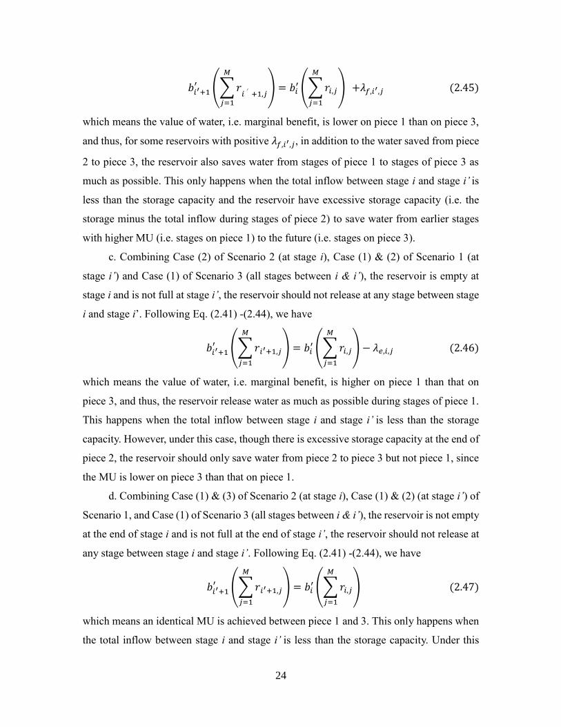
stage i and stage i’. Following Eq. (2.41) -(2.44), we have
24
𝑏𝑖′+1′ (∑𝑟
𝑖′+1,𝑗
𝑀
𝑗=1
) = 𝑏𝑖′ (∑𝑟𝑖,𝑗
𝑀
𝑗=1
) +𝜆𝑓,𝑖′,𝑗 (2.45)
which means the value of water, i.e. marginal benefit, is lower on piece 1 than on piece 3,
and thus, for some reservoirs with positive 𝜆𝑓,𝑖′,𝑗, in addition to the water saved from piece
2 to piece 3, the reservoir also saves water from stages of piece 1 to stages of piece 3 as
much as possible. This only happens when the total inflow between stage i and stage i’ is
less than the storage capacity and the reservoir have excessive storage capacity (i.e. the
storage minus the total inflow during stages of piece 2) to save water from earlier stages
with higher MU (i.e. stages on piece 1) to the future (i.e. stages on piece 3).
c. Combining Case (2) of Scenario 2 (at stage i), Case (1) & (2) of Scenario 1 (at
stage i’) and Case (1) of Scenario 3 (all stages between i & i’), the reservoir is empty at
stage i and is not full at stage i’, the reservoir should not release at any stage between stage
i and stage i’. Following Eq. (2.41) -(2.44), we have
𝑏𝑖′+1′ (∑𝑟𝑖′+1,𝑗
𝑀
𝑗=1
) = 𝑏𝑖′ (∑𝑟𝑖,𝑗
𝑀
𝑗=1
) − 𝜆𝑒,𝑖,𝑗 (2.46)
which means the value of water, i.e. marginal benefit, is higher on piece 1 than that on
piece 3, and thus, the reservoir release water as much as possible during stages of piece 1.
This happens when the total inflow between stage i and stage i’ is less than the storage
capacity. However, under this case, though there is excessive storage capacity at the end of
piece 2, the reservoir should only save water from piece 2 to piece 3 but not piece 1, since
the MU is lower on piece 3 than that on piece 1.
d. Combining Case (1) & (3) of Scenario 2 (at stage i), Case (1) & (2) (at stage i’) of
Scenario 1, and Case (1) of Scenario 3 (all stages between i & i’), the reservoir is not empty
at the end of stage i and is not full at the end of stage i’, the reservoir should not release at
any stage between stage i and stage i’. Following Eq. (2.41) -(2.44), we have
𝑏𝑖′+1′ (∑𝑟𝑖′+1,𝑗
𝑀
𝑗=1
) = 𝑏𝑖′ (∑𝑟𝑖,𝑗
𝑀
𝑗=1
) (2.47)
which means an identical MU is achieved between piece 1 and 3. This only happens when
the total inflow between stage i and stage i’ is less than the storage capacity. Under this

25
case, the excessive storage capability is large enough to regulate water inflow between
piece 1 and piece 3. As a result, some water is saved from piece 1 to piece 3 to achieve
identical MU.
The situation of MU change over some stages, which is not covered above, can be as
follows: piece type (III), (I) and (II) happen consecutively. Under this situation, there might
be a number of decreases of the MU before it reaches a minimum value and then increases
over a number of stages. Similar to the results from Eq. (2.41) – (2.44), it can be proved
that, if a reservoir in the system between stage 𝑖 𝑎𝑛𝑑 𝑖′satisfies: (1) stage 𝑖 is part of piece
type (III) with decreasing MU and stage 𝑖′ is part of piece type (II) with increasing MU; (2)
the reservoir does not release between stage 𝑖 and stage 𝑖′ but releases before stage 𝑖 and
after stage 𝑖′, then the MU is the higher on the piece before stage 𝑖 if the storage of the
reservoir is empty at the end of stage 𝑖; the MU is higher on the piece after stage 𝑖′ if the
storage of the reservoir is full at the end of stage 𝑖′; or the MUs are identical at the stages
before stage 𝑖 and after stage 𝑖′ if the reservoir is neither full at the end of stage 𝑖′ nor empty
at the end of stage 𝑖.
For (II) (as shown in Figure 2.6(II)), reservoirs in the system should operate
following one of the following policy.
a. Combing Case (3) of Scenario 1 (at stage i & i'), and Case (1) of Scenario 3 (all
stages between i & i’), the reservoir is full at the end of both stage i and stage i’. This only
happens when the storage at the beginning of piece 1 plus the total inflow during the stages
of piece 1 is larger than the storage capacity of the reservoir. The capacity limits the
reservoir from saving more water to future stages with higher MU.
b. Combing Case (1) & (2) of Scenario 1 (at stage i), Case (3) of Scenario 1 (at stage
i’) and Case (1) of Scenario 3 (all stages between i & i’), the reservoir is not full at the end
of stage i and is full at the end of stage i’ and the reservoir does not release at any stage of
piece 1. This only happens when the storage at the beginning of piece 1 plus the total inflow
during the stages of piece 1 is less than the storage capacity of the reservoir, and the storage
at the beginning of piece 2 plus the total inflow during stages of piece 2 is larger than the
storage capacity of the reservoir. Thus, to save water for future stages with higher MU, i.e.
stages of piece 3, the reservoir is full at the end of stage i’, and has a preference to save

26
water first from stages of piece 1 with a lower MU than that of piece 2.
c. Combing Case (1) & (2) of Scenario 1 (at stage i& i’) and Case (1) of Scenario 3
(all stages between i & i’), the reservoir is not full at the end of both stage i and stage i’
and the reservoir does not release at any stage of piece 1 and piece 2. This only happens
when the storage at the beginning piece 1 plus the total inflow during the stages of piece 1
and piece 2 is smaller than the storage capacity of the reservoir, thus all inflow during the
stages of piece 1 and piece 2 are saved for the future with higher MU.
For (III) (as shown in Figure 2.6(II)), reservoirs in the system should operate
following one of the following policy.
a. Combining Case (2) of Scenario 2 (at stage i& i’) and Case (1) of Scenario 3 (all
stages between i & i’), the reservoir is empty at the end of both stage i and stage i’. This
indicates that there is abundant inflow during stages after stage i’, so that all water should
be released to make space for the coming inflow.
b. Combining Case (2) of Scenario 2 (at stage i), Case (1) & (3) of Scenario 2 (at
stage i’) and Case (1) of Scenario 3 (all stages between i & i’), the reservoir is empty at
the end of stage i, and is not empty at the end of stage i’, and does not release at any stage
of piece 3. This indicates that the capacity of the reservoir is large enough to save some
inflow during the stages of piece 2 and all inflow during the stages of piece 3 to a future
stage with MU greater or equal to that of piece 2 but smaller than that of piece 1.
c. Combining Case (1) & (3) of Scenario 2 (at stage i & i’) and Case (1) of Scenario
3 (all stages between i & i’), the reservoir is not empty at the end of both stage i and stage
i’, and does not release at any stage of both piece 2 and piece 3. This indicates the
capacity of the reservoir is large enough to save some inflow during the stages of piece 1
and all inflow during the stages of piece 2 & 3 to a future stage with MU greater than or
equal to that of piece 1.
The basic idea of reservoir operation is to save water during water abundant stages
when the MU is lower to water stress stages when the MU is higher. Ideally, if the reservoir
storage is large enough, the MU should be identical over stages with an optimal solution.
However, as the reservoir capacity is limited, the actual optimal solution will result in full-

27
empty cycles of storage with identical MU between two consecutive full-empty stages and
MU changes at empty or full states, i.e., the reservoir releases to empty when the MU
decreases and the reservoir stores water to full when the MU increases. Similarly, for a
system with multiple reservoirs in parallel, full-empty cycles exist as a result of the limited
storage capacity of the reservoirs in the system, i.e., a full storage state of a reservoir might
match together with increasing MU as part of the optimal operation policy; or an empty
state of a reservoir might match together with a decreasing MU. However, according to our
analysis, other conditions, i.e., no release before the MU increases or after the MU
decreases can also match together with the changes of the MU as part of the optimal policy.
It can be showed that at least one reservoir in the system will have either full or empty
storage for the increased or decreased MU, i.e., the storage is the limiting factor which
prevents the reservoir from saving more water from one to another stage to achieve an
identical MU as required by the economic principle. That is to say, the fundamental cause
of the change of MU is the capacity of the reservoirs. However, due to the diversity of
reservoirs in the system, there might also exist some reservoirs with extra-large capacity or
relatively small inflow, such that the capacity of the reservoir is not limiting the reservoir
from saving water to a future stage. As a result, all inflow of those reservoirs can be saved
during stages with high inflow or low demand. Such reservoirs, as shown in Eq. (2.41) –
(2.44), can regulate water over a longer period than the reservoirs with a limited capacity;
they have less frequent full-empty cycles. Therefore, in a system with multiple reservoirs
in parallel, the fundamental cause for MU changes is the limited capacity, while the
difference in capacity and inflow of reservoirs in the system leads to different water
regulation abilities, which results in asynchronized full-empty cycles among reservoirs. On
the other hand, though asynchronized full-empty cycles might exist among different
reservoirs, for those reservoirs that do not become full or empty at certain stages, it must
be have a capacity that is large enough to store all water during stages with high inflow or
low demand, to achieve optimality.
Ideally, if all reservoirs in the system have the same ability to regulate inflow, they
will produce synchronized full-empty cycles as if they are combined into a single reservoir.
Based on principles of optimization, the optimal operation policy for such a virtual single
reservoir (which is equivalent to an optimization problem obtained from original

28
optimization problem by removing the constraint set by the multiple reservoir fact) should
be the best possible optimal solution that the actual parallel reservoir system could achieve
when considering the fact of multi-reservoir system. However, for some reservoirs with
extreme large capacity or extreme small inflow, it is impossible for them to become full
even if they do not release any water before the full storage states of other reservoirs and,
for the same reason, these reservoirs might also not need to synchronize their empty storage
stage with other reservoirs. Under these situations, the actual optimal solution will deviate
from that resulting from the virtual single reservoir.
As a summary, the optimal operation policy for a reservoir system in parallel have
the following properties: (1) the MU evaluated at the demand site is a piece-wise function,
with horizontal pieces, representing a number of consecutive stages with identical MUs,
linked by either increasing pieces (indicating the water demand is becoming less satisfied)
and decreasing pieces (indicating the water demand is becoming more satisfied). The water
demand satisfactory level is affected by various factors including demand levels, inflow
conditions, and reservoir storage capacities. (2) Based on the relationship between the
inflow and the storage capacity, different reservoirs behave differently when the MU
changes; (3) for reservoirs with relatively small inflow and large capacity, if they do not
release at all during a number of consecutive wet stages with high inflow or low demand,
they can be not full when the MU increases after the wet stages or not empty when the MU
decreases before the wet stages, as they have sufficient capacity to save all inflow during
the wet stages to future dry stages with low inflow or high demand; specially, these
reservoirs can regulate water between dry stages with higher MU before and after a number
of consecutive wet stages with lower MU, the maximum amount of water can be saved
from the earlier dry stage to the later dry stage is the excessive storage capacity of the
reservoirs after storing as much water as possible during the wet stages; (4) for normal
reservoirs (reservoirs other than those in (3)), they become full when the MU increases and
become empty when the MU declines, which is due to the limitation of their capacity.

29
2.3 Algorithm Development
Any solution that satisfies the KKT conditions (Eq. (2.6) – Eq. (2.14)) will be the
optimal solution for the reservoir systems with a concave objective function and linear
constraints. Following this property, we design an algorithm to solve the parallel reservoir
system problem.
Based on the discussion above, we solve the optimization problem under the
assumption (Assumption I) that all reservoirs will release as much water as possible before
a decrease in MU, i.e., all reservoir storages achieve the minimum possible value when the
MU decreases, and do not save water for future droughts. The following properties (see
proofs in Appendix B) from the theoretical analysis are used to develop the solution
algorithm: (1) if all reservoirs become full at the first occurrence of MU increase in the study
horizon with the optimal solution solved with Assumption I, then, the optimal release
decision before the reservoirs are full solved with Assumption I will not be subject to
Assumption I. This is because, under this case, there is no reservoir with extra capacity to
save water for the future at the first occurrence of MU increase; thus, no more water can be
saved from stages before the first occurrence of the MU increase to the future; (2) If in the
optimal decisions solved with Assumption I, there is no decrease of MU before the first
occurrence of MU increase (i.e., there is a single MU before the first occurrence of the MU
increase), then, the optimal release decision before the first occurrence of MU increase will
be the same as the optimal release decision of the original problem that is not subject to
Assumption I. This is because under this condition, with the optimal decision solved under
Assumption I, at the first occurrence of the MU increase, reservoirs are either full or not
releasing at all before that stage, so as much as water is saved before the first occurrence of
the increase of the MU, and no more water can be saved for future droughts even with
reservoirs having extra capacity; (3) if no states with increasing MU happens in the optimal
release decision solved with Assumption I, then the optimal release decision will be the same
as the optimal decision of the original problem that is not subject to Assumption I. This is
because under this case, the MU is non-increasing through the whole study horizon; thus,
after removing Assumption I from the optimal release decision solved under Assumption I,
there is no need to save water for the future when MU decreases, as much water as possible

30
should be used in the current periods which are drier compared to the future. (4) if neither
the condition of (1), (2) nor (3) are satisfied in the optimal release decision under Assumption
I, then the optimal release decision between the first occurrence of the MU increase and the
adjacent previous occurrence of the decrease of the MU will be the same as the optimal
release decision of the original problem that is not subject to Assumption I. Under this case,
after removing Assumption I from the optimal release decision solved under Assumption I,
though water might be saved from the stages before the adjacent occurrence of the MU
decrease to the stages after the first occurrence of the MU increase, the water will not be
used between the first occurrence of the MU increase and the adjacent previous occurrence
of the MU decrease as this period has the lowest MU of water before the first occurrence of
increasing MU.
Based on the analysis above, an algorithm is developed to solve the optimal solution
of a system of reservoirs in parallel, as shown below:
(1) Assume all reservoirs will release as much water as possible before a decrease in
MU, i.e., all reservoir storage achieves a minimum possible value when the MU decreases
(Assumption I), that is, all reservoirs release as much as possible for the current stage
without considering future demand. Following the analysis above, a reservoir in the system
either becomes full when the MU increases, or does not release during the water abundant
stages before the MU increases. Solve for the optimal solution up to the first occurrence of
the increase in MU.
Sub-steps under Step (1) under Assumption I are described as follows.
(1-1) Starting from the first stage, calculate the range of the MU [𝜆𝑖, �̅�𝑖], where 𝜆𝑖
refers to the ending storages specified by Eq. (2.48), i.e., the storage at stage i is the storage
capacity of the reservoir if the total water available up to stage i is greater or equal to the
capacity, otherwise, the storage is set to the total inflow from the first stage to stage i, and
�̅�𝑖 refers to the ending storages specified by Eq. (2.49), i.e., the lowest possible storage
while ensuring the ending storage constraints are not violated. Especially, for the last stage
N, there is a single value for with a given ending storage.

31
𝑠𝑖,𝑗 =
{
𝐾𝑗 𝑖𝑓 ∑ 𝐼𝑘,𝑗
𝑖
𝑘=1
+ 𝑠0,𝑗 ≥ 𝐾𝑗
∑𝐼𝑘,𝑗
𝑖
𝑘=1
+ 𝑠0,𝑗 𝑖𝑓 ∑ 𝐼𝑘,𝑗
𝑖
𝑘=1
+ 𝑠0,𝑗 < 𝐾𝑗
,
𝑓𝑜𝑟 𝑖 = 1,2, … ,𝑁 − 1, 𝑗 = 1,2, …𝑀 (2.48)
𝑠𝑖,𝑗 = max {0, 𝑠𝑁,𝑗 − ∑ 𝐼𝑘,𝑗
𝑁
𝑘=𝑖+1
} , 𝑓𝑜𝑟 𝑖 = 1,2, … ,𝑁 − 1, 𝑗 = 1,2, …𝑀 (2.49)
For both cases, the utility is identical before stage i, i.e., 𝜆𝑖 and �̅�𝑖 are the solution of Eq.
(2.50) & Eq. (2.51),
𝑏1′ (𝑟1) = 𝑏2
′ (𝑟2) = ⋯ = 𝑏𝑖′(𝑟𝑖
∗) = 𝜆𝑖 (2.50)
∑𝑟𝑘
𝑖
𝑘=1
=∑∑𝐼𝑘,𝑗
𝑀
𝑗=1
𝑖
𝑘=1
+∑𝑠0,𝑗
𝑀
𝑗=1
−∑𝑠𝑖,𝑗
𝑀
𝑗=1
(2.51)
where 𝜆𝑖 is either 𝜆𝑖 or �̅�𝑖 depending on the storage at the end of stage i as specified above,
𝑟𝑖 is the total release of all reservoirs at stage i (Eq. (2.52)).
𝑟𝑖 =∑𝑟𝑖,𝑗
𝑀
𝑗=1
, 𝑓𝑜𝑟 𝑖 = 1,2, … ,𝑁 (2.52)
(1-2) Starting from the first stage, identify the intersection of the ranges of the MU
before stage i, ⋂ [𝜆𝑘, �̅�𝑘]𝑖𝑘=1 . As ⋂ [𝜆𝑘, �̅�𝑘]
𝑖𝑘=1 ⊂ [𝜆𝑘, �̅�𝑘] for 𝑘 = 1,2, … , 𝑖, thus, a uniform
MU in the range of ⋂ [𝜆𝑘, �̅�𝑘]𝑖𝑘=1 for all stages from the first stage to stage i can ensure that
the storage of any reservoir storage falls in a feasible range (i.e., between 0 and the storage
capacity, and ensuring the ending storage constraint not violated) for 𝑘 = 1,2, … , 𝑖.
At stage i, if
⋂[𝜆𝑘, �̅�𝑘]
i
k=1
= Φ (2.53)
then, there does not exist any single MU value over all stages before i and thus either the
empty or full storage constraint is binding between the beginning and stage 𝑖. Then, one of
the following cases (a-c) will happen.
(a) If Eq. (2.53) is first satisfied at stage i and 𝜆𝑖 > min{�̅�1, �̅�2, … , �̅�𝑖−1}, there does

32
not exist any single MU value over all stages before i, and MU increases at some stages
before i. Assume the first occurrence of MU increase happens at the end of stage 𝑖𝑓, then,
before 𝑖𝑓 there are stages with high inflow compared to demand and after 𝑖𝑓 there are stages
with low inflow compared to demand. Thus, water should be saved as much as possible
during the stages with high inflow, and correspondingly, the MU before 𝑖𝑓 should be as
high as possible. Thus, we have �̅�𝑖𝑓 = min{�̅�1, �̅�2, … , �̅�𝑖−1}, and thus, 𝑖𝑓 can be determined.
Then, the optimal system level release decision before 𝑖𝑓 can be calculated using Eq. (2.48)
– (2.52) by applying these equations from the beginning to 𝑖𝑓, and the storages at the end
of 𝑖𝑓 are specified by Eq. (2.48).
(b) If Eq. (2.53) is satisfied and �̅�𝑖 < max{𝜆1, 𝜆2, … , 𝜆𝑖−1}, there does not exist any
single MU value over all stages before i, and MU decreases at some stages before i. Assume
the first occurrence of the decrease of the MU happens at the end of stage 𝑖𝑒, then, before
𝑖𝑒 there are stages with low inflow compared to demand and after 𝑖𝑒 there are stages with
high inflow compared to demand. Thus, water should be released as much as possible
during the stages with low inflow, and correspondingly, the MU before 𝑖𝑒 should be as low
as possible. Thus, we have �̅�𝑖𝑒 = min{�̅�1, �̅�2, … , �̅�𝑖−1} , and thus, 𝑖𝑒 can be determined.
Then, the optimal system level release decision before 𝑖𝑒 can be calculated using Eq. (2.48)
– (2.52) by applying theses equations from the beginning to 𝑖𝑒, and the storages at the end
of 𝑖𝑒 are specified by Eq. (2.49).
(c) Otherwise, if Eq. (2.53) is not satisfied at all stages, a single MU could be obtained
at all stages without violating any constraints. Then, the optimal system level release
decision can be calculated using Eq. (2.50) – (2.52) by applying theses equations from the
beginning to last stage.
(1-3) Under case (a), release decision up to the first occurrence of the increase of the
MU can be determined, and continues to step (2); under case (b), release decision up to the
first occurrence of the decrease of the MU can be determined (at the end of stage 𝑖𝑒), and
the release decision for the rest of the study period will be solved by solving the problem
from stage 𝑖𝑒 + 1 to the end of the study horizon again using the algorithm in step (1) and
setting the initial storages as empty, until the first occurrence of the increase of the MU is
determined or the last stage is achieved; under case (c), entire release decisions are solved.

33
(2) Based on the solution solved from step (1) under Assumption I, one of the
following steps will be undertaken. These steps follow the discussion at the beginning of
this section.
(a) If there is a stage (i) with constant MU over all stages before the stage (i), break
the entire study horizon into two parts, part 1 covers stages 1 to i; part 2 covers the rest.
The optimal solution of part 1 will be the same as the optimal solution solved from the
problem under Assumption I. For part 2, set the initial storage of all reservoirs as the
corresponding storage at the time when the MU is first increased in the optimal solution
solved from the problem under Assumption I, and set the new study horizon from the first
occurrence of the increase of the MU to the end of the study horizon, and solve the problem
again using this algorithm.
(b) if there is a stage with increasing MU and all reservoirs are full at the first
occurrence of MU increase, then, break the entire study horizon into two parts, stages
before the first occurrence of MU increase (part 1) and the rest of study period (part 2).
The optimal solution of part 1 will be the same as the optimal solution solved from the
problem under Assumption I. For part 2, set the initial storage of all reservoirs as their
capacity, and set the new study horizon from the first occurrence of the MU increase to the
end of the original study horizon, and solve the problem again using this algorithm.
(c) if the final stage is achieved without increasing MU at any stage, then, the release
decision will be the same as that under Assumption I, and the algorithm stops.
(d) if none of (a) – (c) satisfies, then the optimal release decision between the first
occurrence of the increasing MU and the adjacent previous occurrence of the decreasing
MU can be determined, and the release decisions at other stages are solved by solving the
following problem again using the algorithm. Assuming the first occurrence of an
increasing MU happens at the end of stage 𝑖𝑓 and the adjacent previous occurrence of a
decrease MU happens at the end of stage 𝑖𝑒, the problems is stated as follows: Take the
stages from the beginning to the end of 𝑖𝑒 and the stages from the end of 𝑖𝑓 to the end of
the study period (which is defined as a sub-study horizon). Set the storage capacity at the
end of 𝑖𝑒 as the remaining storage capacity defined as Eq. (2.54) and set the inflow at the
stage after 𝑖𝑒 in the new problem, which is the stage after 𝑖𝑓 in the original problem as Eq.

34
(2.55),
𝐾𝑖𝑒,𝑗𝑛𝑒𝑤 = 𝐾𝑗
𝑜𝑟𝑖 − 𝑠𝑖𝑓,𝑗𝐴 (2.54)
𝐼𝑖𝑒+1,𝑗𝑛𝑒𝑤 = 𝐼𝑖𝑓+1,𝑗
𝑜𝑟𝑖 + 𝑠𝑖𝑓,𝑗𝐴 (2.55)
where, 𝐾𝑖𝑒,𝑗𝑛𝑒𝑤, 𝐼𝑖𝑒+1,𝑗
𝑛𝑒𝑤 are the storage capacity of reservoir j at the end of 𝑖𝑒 and the inflow
at the stage after 𝑖𝑒 to reservoir j in the new problem respectively, 𝐾𝑗𝑜𝑟𝑖 and 𝐼𝑖𝑓+1,𝑗
𝑜𝑟𝑖 are the
storage capacity of reservoir j and the inflow at the stage after 𝑖𝑓 to reservoir j in the original
problem, respectively, and 𝑠𝑖𝑓,𝑗𝐴 is the ending storage of reservoir j at the end of stage 𝑖𝑓 in
the optimal solution of the original problem under Assumption I. This step follows the fact
that the optimal release decision between the first occurrence of an increasing MU and the
adjacent previous occurrence of a decreasing MU in the optimal solution under Assumption
I will be the same as the optimal release decision of the original problem without
Assumption I, and also that if there are two periods (P1 and P2) with higher MU before
and after a period (P3) with lower MU, and there is remaining storage capacity at the end
of P3, i.e., some reservoirs are not full at the end of P3, then P1 and P2 will achieve a
uniform MU by saving water from P1 to P2, but the maximum amount of water saved from
P1 and P2 is constrained by the remaining storage capacity at the end of P3.
(3) After step 2, the system level releases are determined, and also, we determine full
and empty states for all reservoirs, and thus we can determine the total release of each
reservoir between each pair of consecutive full/empty states by simply applying the mass
balance relationship. As long as the operation activity follows these two requirements, the
release decisions are always optimal. As we explicitly consider the constraints when
solving for the optimal solution, it is ensured that a feasible solution will exist.
2.4 Case Study
To demonstrate the solution algorithm applied to the operation of a parallel reservoir
system, a simple synthetic case is presented as follows. Inflow data for a system consisting
of 5 parallel reservoirs is synthesized by the Thomas-Fiering model (Thomas & Fiering,
1962),

35
𝑞𝑖+1 = 𝜇 + 𝜌𝑓𝑙𝑜𝑤(𝑞𝑖 − 𝜇) + √1 − 𝜌𝑓𝑙𝑜𝑤2 (𝜇𝐶𝑣)𝜔 (2.56)
where 𝑞𝑖 is the inflow at stage i, 𝜇 is the average inflow an is set as 1 for reservoirs 1-4 and
0.1 for reservoir 5, which is also set as the initial inflow at the first stage, 𝜌𝑓𝑙𝑜𝑤 represents
the temporal correlation of the inflow and is set as 0.3 for all reservoirs, and 𝐶𝑣 represents
the inflow variability and is set as 0.5 for all reservoirs, and 𝜔 is a random number
generated from standard normal distribution. For simplicity, a constant demand 1 is used
at all stages, a uniform storage capacity 2 is applied to all reservoirs, and the MU function
𝑏′(⋅) is assumed to be a function of release/demand ratio with the same form at all stages,
i.e.,
𝑏𝑖′(𝑟𝑖) = 𝑏′ (𝑟𝑖𝑑𝑖) (2.57)
where, 𝑟𝑖 is the release at stage i, 𝑑𝑖 is the demand at stage i.
Figure 2.7 shows the optimal release schedule given by the algorithm. The top figure
shows the MU over stages, and the middle figure shows the system level releases over
stages, and the bottom figure shows the individual reservoir release schedule, which
consists of empty states (blue stars), full states (red circles), no release stages (grey color),
and the total release (numbers) between two consecutive empty/full states. As can be seen,
all reservoirs become empty at stage 21, when the MU decreases, and all reservoirs become
full at stage 33, when the MU increases, and reservoirs 1-4 become full at stage 31 and
reservoir 5 does not release before stage 31, which is a stage with an increasing MU.
Furthermore, reservoir 5 is empty at stage 21 and not full at stage 31 with no release
between the two stages, which corresponds to the higher MU at stage 20 than that at stage
32. The results from the algorithm satisfy all the requirements derived from the theoretical
analysis.

36
Figure 2.7 Optimal release schedule given by the algorithm (top figure: MU over
stages, middle figure: system level releases over stages, bottom figure: individual
reservoir release schedule)
Based on the optimal release schedule shown in Figure 2.7, the system level release
schedule can be further broken down into individual release schedules. As there usually
exist numerous optimal individual release schedules, reservoir operators might decide their
own release schedule based on their own preference. For this case study, we derive the
individual release schedule according to the following rules: (1) reservoirs with shorter
full-empty cycle has a higher priority to release, i.e., in this case study, reservoir 1-4 release
first before reservoir 5; (2) for the reservoirs with the same release priority, the release from
each reservoir is proportional to the total available water of that reservoir. Following these
two rules, the individual reservoir releases are determined as Figure 2.8(a), and the storages
shown in 2.8(b). Further, as shown in Figure 2.9, the system level release given by the
individual releases shown in Figure 2.8(a) provides the same system level release as
required by the optimal solution given by the algorithm. Thus, individual releases shown
in Figure 2.8(a) actually provides one set of optimal individual release decisions. Note
these two rules do not always guarantee one set of feasible optimal solution, especially
when there exist extremely high inflows to some reservoirs, but with a few more
adjustments, a set of feasible solution can be obtained.

37
(a) Individual releases
(b) Individual storages
Figure 2.8 Individual releases and storages

38
Figure 2.9 Validation of the individual releases
2.5 Conclusions
In this chapter, a multi-stage optimization model is set up to derive the properties of
the optimal release decision for a system of reservoirs in parallel with a single demand site.
Analytical analysis is conducted using KKT conditions. We show that the optimal
operation policy for such as a reservoir system has the following properties: (1) the MU
evaluated at the demand site changes with time according to the inflow condition, demand
level, etc., in a piece-wise form. (2) based on the relationship between the inflow and the
storage capacity, different reservoirs behave differently when the MU changes; (3) for
reservoirs with relatively small inflow and large capacity, if they do not release at all during
wet stages with low demand, they can be not full when the MU increases after the wet
stages or not empty when the MU decreases before the wet stages, as they have sufficient
capacity to save water from the wet stages to future dry stages with high demand; specially,
these reservoirs can regulate water between dry stages with higher MU before and after a
number of consecutive wet stages with lower MU, the maximum amount of water can be
saved from the earlier dry stage to the later dry stage is the remaining storage capacity of

39
the reservoirs after storing as much water as possible during the wet stages; (4) for normal
reservoirs (reservoirs other than those in (3)), they become full when the MU increases
empty when the MU decreases, which is due to the limitation of their capacity.
Furthermore, based on the understanding of the properties of the optimal solution for
a system of reservoirs in parallel, an algorithm is developed to solve the optimization model
defined for such a system with a single demand site. The algorithm follows the properties
derived from the KKT conditions. The algorithm can be applied to solve parallel reservoir
operation problems with computational efficiency. A synthetic case study is conducted to
show the application of the algorithm with effectiveness and validity.

40
CHAPTER 3: DETERMINING EFFECTIVE
FORECAST HORIZON
3.1 Introduction
Inflow forecast is important for making reservoir operation decisions, while
imperfect forecast might significantly reduce the usefulness of the forecast information
(Mishalani and Palmer, 1988). Among the previous studies, You and Cai (2008) developed
a theoretical relationship based on dimensional analysis for determining the forecast
horizon, which is a length of the forecast beyond which the inflow will no longer affect the
release decision in the decision horizon. Zhao et al. (2012) conducted numerical
experiments with imperfect forecast and proposed the concept of effective forecast horizon
with a certain level of uncertainty, which provides maximum information to support
reservoir operation decisions. In general, the effective forecast horizon becomes shorter as
forecast uncertainty increases. This study continues the efforts listed above. We analyze the
optimal release decision using a multi-stage reservoir operation model and develop
numerical procedures to determine the effective forecast horizon (EFH). This study enables
reservoir operation decision makers to fully use inflow forecast while controlling the
forecast uncertainty.
In this work, we follow the following procedures to develop the criteria and
procedures to identify the EFH under a given uncertainty level. First, we set up a
deterministic model to discuss the characteristics of optimal multistage reservoir operation
solutions. Then, the relationship between the uncertain inflow forecast and the optimal
release decisions are explored, i.e., the lower bound and upper bound of the optimal release
decisions over all possible inflow scenarios. Following that, we will establish a criterion to
examine whether the forecast heading period of any given forecast can be a candidate of
the EFH or not. Finally, the overall procedures for determining EFH are proposed.
3.2 The Mathematical Model
A deterministic optimization model is first set up for multi-stage reservoir operation

41
to optimize the utility function over all time period with mass balance, non-negative storage
and reservoir capacity as constraints (Draper and Lund, 2004; You and Cai, 2008a, 2008b).
The results of the deterministic optimization model will be used to prove the criteria to be
established for the EFH and to design an algorithm to determine the EFH considering
inflow uncertainty. The solution of this model provides the “ideal” optimal release decision
for the formulated problem. For simplicity, water loss from the reservoir such as
evaporation and leakage are ignored in the analysis without loss of significance.
Obj. max∑𝑏𝑖(𝑟𝑖) (3.1)
𝑠. 𝑡.
𝑠𝑖−1 + 𝐼𝑖 − 𝑟𝑖 = 𝑠𝑖, 𝑓𝑜𝑟 𝑖 = 1,2, … ,𝑁 (3.2)
𝑠𝑖 ≥ 0, 𝑓𝑜𝑟 𝑖 = 1,2, … ,𝑁 (3.3)
𝑠𝑖 ≤ 𝐾, 𝑓𝑜𝑟 𝑖 = 1,2, … ,𝑁 (3.4)
where 𝑏𝑖(𝑟𝑖) is the concave utility function for stage i, 𝑠𝑖 is the storge of reservoir at the
end of stage i, 𝐼𝑖 is the inflow forecast during stage i, 𝑟𝑖 is the release during stage i, K is
the capacity of the reservoir and N is the attempted forecast horizon.
Applying the KKT conditions (Bazaraa et al., 2013) to the model described above,
we obtain the following general conditions for an optimal solution (see Appendix C for
detailed derivation.)
−𝜕𝑏𝑖(𝑟𝑖)
𝜕𝑟𝑖+ 𝜆𝑏,𝑖 = 0, 𝑓𝑜𝑟 𝑖 = 1,2, … , 𝑁 (3.5)
𝜆𝑏,𝑖−1 − 𝜆𝑏,𝑖 − 𝜆𝑒,𝑖 + 𝜆𝑓,𝑖 = 0, 𝑓𝑜𝑟 𝑖 = 2,… ,𝑁 (3.6)
where 𝜆𝑒,𝑖 is the marginal price for non-negative storage constraints, 𝜆𝑓,𝑖 is the marginal
price for capacity constraints and 𝜆𝑏,𝑖 is the marginal price for mass balance constraints.
In the following, we discuss the various forms of Eq. (3.5) and (3.6) under different
conditions of binding/unbinding constraints. We use the cumulative inflow curve and
cumulative water delivery curve, which are used in the classic Rippl’s curve (Ripple, 1883),
to illustrate the conditions and associated optimal releases. Three cases for stage i and stage
i+1 are discussed, including both capacity and non-negative storage constraints unbinding,
the non-negative storage constraint binding, and the storage capacity constraint binding.

42
Case 1: Both capacity and non-negative storage constraints are unbinding
With unbinding capacity and non-negative storage constraints,
𝜆𝑒,𝑖 = 0 (3.7)
𝜆𝑓,𝑖 = 0 (3.8)
Substitute Eq. (3.7) and (3.8) to Eq. (3.5) and (3.6),
𝑏𝑖′(𝑟𝑖
∗) =𝜕𝑏𝑖𝜕𝑟𝑖
= 𝜆𝑏,𝑖 (3.9)
𝑏𝑖′(𝑟𝑖
∗) = 𝜆𝑏,𝑖 = 𝜆𝑏,𝑖+1 = 𝑏𝑖+1′ (𝑟𝑖+1
∗ ) (3.10)
which means that the marginal utility (MU), i.e. economic value of water, which might be
affected by several factors including the inflow conditions and the demand, are identical
between stage i and stage i+1. Under this scenario, the reservoir is large enough to regulate
the inflow to the reservoir to match the demands on both stages, and the economic principal
is followed, i.e. identical MU between two stages (Figure 3.1(a)).
Case 2: Only the non-negative storage constraint is binding
Assuming the non-negative storage constraints become binding at stage i,
𝜆𝑒,𝑖 > 0 (3.11)
and the capacity constraint is unbinding,
𝜆𝑓,𝑖 = 0 (3.12)
Substitute Eq. (3.11) and (3.12) to Eq. (3.5) and (3.6),
𝜆𝑏,𝑖 = 𝜆𝑏,𝑖+1 + 𝜆𝑒,𝑖 (3.13)
𝑏𝑖′(𝑟𝑖
∗) = 𝑏𝑖+1′ (𝑟𝑖+1
∗ ) + 𝜆𝑒,𝑖 (3.14)
According to Eq. (3.14), with the optimal solution, the marginal utility (MU), i.e. the
economic value of water, will decrease right after the empty storage state, indicating the
system state shifting from a water short stage, i.e., water supply is limited compared to
water demand, to a water abundant stage, i.e., water supply is sufficient compared to water
demand. The relatively low inflow or relatively high demand at stage i require the reservoir
to release as much water as possible, and thus the reservoir storage reaches to the empty
state at the end of stage i (Figure 3.1(b)), associated with a relatively large MU before the
empty state.

43
Case 3: Only the storage capacity constraint is binding
Assuming the storage capacity constraints become binding at stage i,
𝜆𝑓,𝑖 > 0 (3.15)
and the non-negative constraint is unbinding, i.e.,
𝜆𝑒,𝑖 = 0 (3.16)
Substitute Eq. (3.15) and (3.16) to Eq. (3.5) and (3.6),
𝜆𝑏,𝑖−1 = 𝜆𝑏,𝑖 − 𝜆𝑓,𝑖 (3.17)
𝑏𝑖−1′ (𝑟𝑖−1
∗ ) = 𝑏𝑖′(𝑟𝑖
∗) − 𝜆𝑓,𝑖 (3.18)
Under the optimal release decision, the MU will increase right after full storage occurs,
indicating the system shifts from a water abundant stage, where the water supply is
sufficient compared to water demand, to a water short stage, where the water supply is
limited compared to water demand. The relatively high inflow or the relatively low demand
at stage i require the reservoir to store as much water as possible to stage i+1, and thus the
reservoir storage reaches full at the end of stage i (Figure 3.1(c)) associated with a relatively
small MU before the full state.
Taking all these three cases into consideration of the whole study horizon (N stages),
the MU can be plotted by horizontal pieces linked by either an increasing or a decreasing
piece with a slope. Each horizontal piece corresponds to a number of consecutive stages
where the reservoir is usually neither full nor empty but the starting or ending point of each
horizontal piece corresponds to either an empty or a full storage states (except for the first
piece which starts from the given initial storage and the last piece which ends with the
ending storage). Each increasing piece (with a nonlinear monotonically increase trend)
corresponds to a number of consecutive stages with full ending storage, and each
decreasing piece (with a nonlinear monotonically decrease trend) corresponds to a number
of consecutive stages with empty ending storage. Specially, if two horizontal pieces are
linked by only one stage with either full or empty ending storage, the increasing piece or
decreasing piece becomes vertical. In summary, the reservoir storage states (including the
empty/full cycles) correspond to piece-wise curves of MU, which are linear except for the
case of consecutive empty/full storage over a number of stages.
For each horizontal piece containing 𝑁𝐻 stages ( 𝑖 = 𝑖𝑘+1, 𝑖𝑘+2, … , 𝑖𝑘+𝑁𝐻 ), the
marginal utilities at any two consecutive stages follow Eq. (3.10), which gives 𝑁𝐻𝑃 − 1

44
equations with 𝑁𝐻 unknows, i.e., the release (𝑟𝑖∗ ) during the 𝑁𝐻 stages. The initial and
ending storage of the reservoir on the horizontal piece, 𝑠𝑃0 and 𝑠𝑃𝑁, should take empty
storage, full storage, initial storage (𝑠0) or ending storage (𝑠𝑁), thus according to the mass
balance on a horizontal piece, Eq. (3.19) could be obtained.
∑ 𝑟𝑗
𝑖𝑘+𝑁𝐻𝑃
𝑖=𝑖𝑘+1
= ∑ 𝐼𝑗
𝑖𝑘+𝑁𝐻𝑃
𝑖=𝑖𝑘+1
+ 𝑠𝑃0 − 𝑠𝑃𝑁 (3.19)
Combining the 𝑁𝐻𝑃 − 1 equations given by Eq. (3.10) and Eq. (3.19), we could obtain 𝑁𝐻𝑃
equations with 𝑁𝐻𝑃 unknowns, and solve for 𝑟𝑖∗ on the piece. For any stage on an
increasing piece, the initial and the ending storage of the stage are both full storage; thus,
according to mass balance, the release should be identical to the inflow on those stages.
Similarly, for any stage on a decreasing piece, the initial storage and empty storage of the
stage are both empty storage; the release should be identical to the inflow on these stages
too. Overall, the release decision over all N stages can be determined by the procedures
described above.
Furthermore, when the storage state turns from a non-empty state to an empty state,
the cumulative release curve must be tangent to the cumulative inflow curve (Figure 3.1(b))
(see the proof of this tangent relationship in Appendix D.) Similarly, when the storage state
turns from a non-full state to a full state, the cumulative release curve should be tangent to
the curve, as shown in Figure 3.1(c), if the cumulative inflow curve is moved downward
by the storage capacity (Figure 3.1(c)).
Based on the three cases shown between two stages as discussed above, two special
cases are further discussed in the following. Case 4: the non-negative storage constraint
becomes binding for the first time after the initial storage, and then the storage capacity
constraint becomes binding at a later stage; and vice versa for Case 5. These two cases
cover multiple stages instead of two as used in Cases 1-3.
Case 4:
Under this case (Figure 3.1(d)), the non-negative storage constraint is binding first
at stage i and then the storage capacity constraint is binding at a later stage j. Before stage
i, the reservoir is neither empty nor full, and the MU relationships follow Eq. (3.10) (i.e.,
Case 1), i.e., the MU is identical from the initial stage up to stage i. At the end of stage i,

45
the reservoir is empty, and possibly continues to be empty until stage k, for which Eq. (3.14)
holds (i.e., Case 2). Along the curve connecting the two horizontal lines (horizontal line
before stage i and line after stage k), the reservoir remains an empty state, the MU declines,
and the reservoir releases all inflow at all stages from stage i+1 to k. Starting from stage
k+1 and before stage j, Eq. (3.10) holds (i.e., Case 1) again as the reservoir is usually neither
full nor empty, and Eq. (3.18) (i.e. Case 3) holds for stage j and the following stages with
full ending storage, and the MU increases from a lower value to a higher value after each
full state. Starting from next stage with non-full ending storage, Eq. (10) holds (i.e., Case
1) again, and so on. At a state of empty storage, the cumulative release curve is tangent to
the cumulative inflow curve; while at a stage of full storage, the cumulative release curve
is tangent to the curve that is the cumulative inflow curve moved downward by the storage
capacity.
Define 𝑇𝑑 as the period from the beginning to the time of the first occurrence of full
(empty) storage and 𝑇𝑓 as the period from the beginning to the time of the first occurrence
of empty (full) storage (Figure 3.1(d), (e)), In this case, if 𝑇𝑑 represents the period from the
beginning to the first occurrence of empty storage and 𝑇𝑓 as the period from the beginning
to the first occurrence of full storage (Figure 3.1(d)). It is proved that as long as the inflow
forecast in 𝑇𝑓 is given, the optimal release decision in 𝑇𝑑 will be determined no matter how
inflow after 𝑇𝑓 will be (See Appendix E). Actually, if the future inflow beyond 𝑇𝑓 is
abundant, it will be better to use more water within 𝑇𝑓 and decrease the water storage at
the end of 𝑇𝑓 as much as possible. Under this situation, within 𝑇𝑑 , the release decision will
not be affected by the inflow beyond 𝑇𝑓, as the storage is empty at 𝑇𝑑 and the water use
within 𝑇𝑑 already reaches the maximum. On the other hand, if there exists water stress in
the future beyond 𝑇𝑓, more water should be left to the future and less water be used within
𝑇𝑓. However, at the end of 𝑇𝑓, if the storage constraint is binding, there is no more capacity
to reserve water to the future. Thus, even if there is a drought event in the future, the optimal
release decision within 𝑇𝑑 will not change. Thus, under the condition of such empty-full
states, forecast is not needed beyond 𝑇𝑓 for the release decision within 𝑇𝑑.
Case 5:
Under this case, the storage capacity constraint becomes binding first, followed by a
46
binding non-negative storage constraint at a later stage. Assuming the storage capacity
constraint becomes binding first at stage i and then the non-negative storage constraint
becomes binding at a later stage j. Before stage i, the reservoir is usually neither empty nor
full, the MU relationships follow Eq. (3.10) (i.e., Case 1), and the MU is identical before
the end of stage i. At the end of stage i, the reservoir is full, and it possibly continues to be
full until after stage k, where Eq. (3.18) (i.e., Case 3) holds. After each of the full storage
states that can occur continuously between stage i and k, the MU increases continuously.
The reservoir releases all inflow between stages i+1 to stage k. Starting from stage k+1 and
before stage j, Eq. (3.10) holds (i.e., Case 1) again as the reservoir is usually neither full
nor empty, and Eq. (3.14) (i.e. Case 2) holds for stage j and the following stages with empty
ending storage, where the MU declines.
Under this case, 𝑇𝑑 represents the period from the beginning to the first occurrence
of full storage state and 𝑇𝑓 as the period from the beginning to the first occurrence of empty
storage (Figure 3.1(e)). As shown in Appendix E, similar to Case 4, it is proved 𝑇𝑓 is the
longest forecast horizon that provide useful information to the release decision within 𝑇𝑑.
This can also be justified as follows: If future has a water deficit situation, less water should
be used within 𝑇𝑓, and thus, the water storage at the end of 𝑇𝑓 will be increased. Under this
situation, only the release decision after 𝑇𝑑 can be changed. This is because the storage
capacity is binding at 𝑇𝑑 , and the capacity of the reservoir limits the ability of the reservoir
to store more water for the future. Under the water abundant situation, the release decision
within 𝑇𝑓 (thus also within 𝑇𝑑) will not be affected by the inflow beyond 𝑇𝑓, as the storage
is empty at 𝑇𝑓, and, water use within 𝑇𝑓 already reaches the maximum. Thus, under the
condition of such full-empty states, forecast is not needed beyond 𝑇𝑓 for the release
decision within 𝑇𝑑.

47
Stage i Stage i+1
Cu
mu
lati
ve I
nfl
ow
/Rele
ase
Marg
inal
Uti
lity
Accumulated InflowAccumulated Release
Legend
Marginal UtilityAccumulated Inflow-K
Storage
(a) Case 1: with the binding mass balance constraint only
Stage i Stage i+1
Cu
mu
lati
ve I
nfl
ow
/Rele
ase
Marg
inal
Uti
lity
S0
(b) Case 2: binding mass balance constraint with binding non-negative storage constraints
Stage i Stage i+1
Cu
mu
lati
ve I
nfl
ow
/Rele
ase
Marg
inal
Uti
lity
K
(c) Case 3: binding mass balance constraint with binding storage capacity constraints
Figure 3.1 Optimal reservoir release under the various cases ((a) to (e)).

48
Figure 3.1 (cont.)
Time (Stages)
Cu
mu
lati
ve I
nfl
ow
/Rele
ase
Marg
inal
Uti
lity
Tf
Td
stage i k stage j
S0
K
(d) Case 4: the non-negative storage constraint binding first and then the storage capacity
constraint binding (the increasing part and decreasing part of MU does not have a specific
shape)
Time (Stages)
Cu
mu
lati
ve I
nfl
ow
/Rele
ase
Marg
inal
Uti
lity
Tf
Td
stage i k stage j
S0
K
(e) Case 5: the storage capacity constraint binding first and then the non-negative storage
constraint binding (the increasing part and decreasing part of MU does not have a specific
shape)
After the first full-empty (empty-full) cycle, such empty-full or full-empty states can
occur multiple times during the study period and the MU relationships and decision rules
discussed above repeat, though it will no longer influence the release decision at the current
stage.

49
3.3 Procedures to Determine Effective Forecast Horizon
The problem of determining the EFH is stated as follows: Given inflow forecast time
series, 𝐼1, 𝐼2, … , 𝐼𝑁 , and corresponding inflow uncertainty, which is given as certain
confidence intervals, such as [𝐼1, 𝐼1̅], [𝐼2, 𝐼2̅], … , [𝐼𝑁 , 𝐼�̅�], the EFH will satisfy the following
condition: the decision error at the current stage does not go beyond a given error bound,
EB, i.e.,
∀𝑅1∗, 𝐸𝐵 ≥ |𝑅1 − 𝑅1
∗| (3.20)
where, 𝑅1 is the optimized release decision at the current stage under forecast with
uncertainty; 𝑅1∗ is the optimal release decision under a perfect forecast, which is usually
unknown given that a perfect forecast does not exist for decision making. EB is the
prescribed error bound.
To determine the EFH, a longest forecast horizon (LFH) is first proposed that
provides useful information for the current stage decision. You and Cai (2008) defined the
forecast horizon as forecast lead time which would enable the optimal release decision in
the decision horizon without any inflow forecast beyond the forecast horizon. Zhao et al.
(2012) showed the existence of such a forecast horizon under imperfect forecast using
numerical experiments. Similarly, we show that there exists a longest forecast horizon
(LFH), beyond which the future inflow information and associated uncertainty will no
longer affect the error involved in the release decision at the current stage, i.e., all forecast
lead time greater or equal to the LFH will result in the same error bound of release decision
at current stage (Figure 3.2). Thus, the LFH will provide the longest possible forecast lead
time as a candidate for the EFH. The LFH is similar as the forecast horizon as discussed in
You and Cai (2008) but characterized by error involved in release decision as shown in
Figure 3.2. As discussed later, if the LFH satisfies the criterion for EFH, then the EFH
should be identical to the LFH; otherwise, the EFH should be shorter than the LFH and it
is conditioned with a given storage at the end of the EFH (i.e., the ending storage).

50
Figure 3.2 Illustration of the EFH and LFH
Assume a concave utility function, 𝑏(𝑟), 𝑏′(𝑟) → 0, when 𝑟 → ∞; 𝑏′(𝑟) → ∞, when
𝑟 → 0. For a given time period, under the most optimistic inflow conditions beyond the
time period, i.e., 𝑟 → ∞, 𝑏′(𝑟) → 0 beyond the time period, then the marginal utility will
decrease at the end of the time period (as the MU approaches 0 after the time period), thus
the ending storage should be empty; under the most pessimistic inflow conditions beyond
the time period, i.e., 𝑟 → 0, 𝑏′(𝑟) → ∞ beyond the time period, then the marginal utility
will increase at the end of the time period (as the MU approaches infinity after the time
period), thus the ending storage should be full. Thus, if the release decision at current stage
is irrelevant to the ending storage specified at the end of the forecast horizon, the release
decision is also irrelevant to the inflow condition beyond the forecast horizon. Thus, the
LFH also represents the shortest forecast lead time which would lead to a release decision
at the current stage with the release error bound irrelevant to the given storage at the end
of the forecast lead time. As shown in Appendix F, assuming that actual inflows stay within
the forecasted range under a given confidence level, with any given ending storage, 𝑆𝑁, as
constraints, the lower bound and the upper bound of the release at the current stage will be
specified by a the most pessimistic and most optimistic inflow scenario. With the most
pessimistic forecast, the cumulative inflow at each stage is lower than the cumulative
inflow over all scenarios; with the most optimistic forecast, the cumulative inflow at each
stage is higher than that over all scenarios. Thus, if the most pessimistic and most optimistic
inflow scenario provide consistent upper bound and lower bound of the optimal release

51
decision at current stage with any given ending storage, then the lower bound and upper
bound of the optimal release will be irrelevant to the ending storage, which also means that,
with given release decision at the current stage made by some reservoir operation policy,
the release error bound at current stage will be irrelevant to the ending storage.
Actually, as shown in Section 3.2 with Case 4 and Case 5, for any inflow scenario,
if there exists full-empty or empty-full cycle in the optimal release decision, then the
decision at the current stage is irrelevant to the forecast beyond the cycle. Thus, if both the
most pessimistic and optimistic inflow scenarios include sufficient variability, i.e.,
including a full-empty or empty-full cycle in the corresponding optimal release decision,
there will exist a LFH.
Thus, two special scenarios, i.e. the most optimistic one or the most pessimistic one,
will be synthesized based on all possible inflow scenarios to determine the LFH. As proved
in Appendix G, for any inflow scenario, if the release decisions at the current stage resulting
from an empty ending storage constraint or a full ending storage constraint are identical,
then the release decisions at the current stage are irrelevant to the ending storage. The
property holds for the most optimistic or the most pessimistic scenario, and thus with
inflow forecast with in LFH,
𝑅1,𝑜𝑝𝑡,𝑓∗ = 𝑅1,𝑜𝑝𝑡,𝑒
∗ (3.21)
𝑅1,𝑝𝑒𝑠,𝑓∗ = 𝑅1,𝑝𝑒𝑠,𝑒
∗ (3.22)
where 𝑅1,𝑜𝑝𝑡,𝑓∗ / 𝑅1,𝑜𝑝𝑡,𝑒
∗ are the release decision at the current stage under the most
optimistic forecast with full/empty ending storage constraint; 𝑅1,𝑝𝑒𝑠,𝑓∗ /𝑅1,𝑝𝑒𝑠,𝑒
∗ are the
release decisions under the most pessimistic forecast. Over all the tested LFH, the shortest
one is selected as the LFH.
Further, the following procedures are proposed to determine the LFH (See the
flowchart shown in Figure 3.3):
(a) Prepare the following input data set: inflow forecast for future N stages, 𝐼1, 𝐼2, … , 𝐼𝑁;
inflow forecast under the most optimistic scenario, 𝐼1,𝑜𝑝𝑡, 𝐼2,𝑜𝑝𝑡, … , 𝐼𝑁,𝑜𝑝𝑡 and the most
pessimistic scenario, 𝐼1,𝑝𝑒𝑠, 𝐼2,𝑝𝑒𝑠, … , 𝐼𝑁,𝑝𝑒𝑠 (following the definition given before);
demand for each stage, 𝐷1, 𝐷2, … , 𝐷𝑁; initial storage at the beginning, 𝑆0; storage capacity
of the reservoir, K; and utility functions for each stage, 𝑏𝑖(⋅).

52
(b) Set the initial candidate of 𝐿𝐹𝐻 as the study horizon (N) (the longest LFH) and examine
whether the 𝐿𝐹𝐻 = 𝑁 satisfies the requirement for LFH, i.e. Eq. (3.21) & (3.22). If not,
then, the LFH should be greater than the study period (N) and the program stops.
Otherwise, 𝑁 − 1 will be set as the candidate for next test. If 𝑁– 1 does not satisfy the
requirement for LFH, then, N remain as the LFH; otherwise, 𝑁– 2 is set as next candidate,
and so on. When 𝑁 − 𝑘 does not stratify the requirement, then 𝑁 − 𝑘 + 1 is the final LFH.
Obtain Data: Inflow Forecast (length N),
Forecast Uncertainty, Demand, Capacity and
Initial Storage.
Start
Set MFH = N
End
Determine the Release Decision at the First Stage:
Under the most optimistic forecast with full ending storage constrain, ,
Under the most optimistic forecast with empty ending storage constraint, ,
Under the most pessimistic forecast with full ending storage constraint, ,
Under the most pessimistic forecast with empty ending storage constraint, .
𝑅1,𝑜𝑝𝑡 ,𝑓∗ = 𝑅1,𝑜𝑝𝑡 ,𝑒
∗
𝑅1,𝑝𝑒𝑠 ,𝑓∗ = 𝑅1,𝑝𝑒𝑠 ,𝑒
∗
𝑅1,𝑜𝑝𝑡 ,𝑓∗
𝑅1,𝑜𝑝𝑡 ,𝑒∗
𝑅1,𝑝𝑒𝑠 ,𝑓∗
𝑅1,𝑝𝑒𝑠 ,𝑒∗
and ?
Yes
No
Yes
LFH = LFH - 1
LFH = N ?
LFH >N
No
LFH = LFH + 1
Figure 3.3 Procedure for Determining the LFH
After the LFH is determined, the following procedures are applied to further
determine EFH. First, we specify the criterion for EFH. With given inflow forecast for
future N stages, 𝐼1, 𝐼2, … , 𝐼𝑁 , and corresponding inflow uncertainty under certain
confidence levels, such as [𝐼1, 𝐼1̅] , [𝐼2, 𝐼2̅], … , [𝐼𝑁 , 𝐼�̅�] , a release decision for the current
stage, 𝑅1, could be made following some reservoir operation policy. With a given error
bound, EB, the requirement for the release decision at the current stage is given by Eq.
(3.20). If an estimate of the unknown actual optimal release decision, 𝑅1∗, could be made,
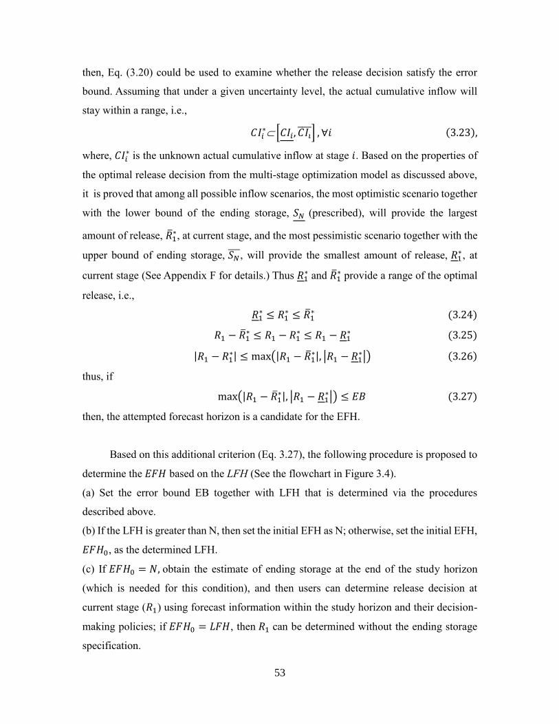
53
then, Eq. (3.20) could be used to examine whether the release decision satisfy the error
bound. Assuming that under a given uncertainty level, the actual cumulative inflow will
stay within a range, i.e.,
𝐶𝐼𝑖∗ [𝐶𝐼𝑖, 𝐶𝐼𝑖̅̅ ̅̅ ] , ∀𝑖 (3.23),
where, 𝐶𝐼𝑖∗ is the unknown actual cumulative inflow at stage 𝑖. Based on the properties of
the optimal release decision from the multi-stage optimization model as discussed above,
it is proved that among all possible inflow scenarios, the most optimistic scenario together
with the lower bound of the ending storage, 𝑆𝑁 (prescribed), will provide the largest
amount of release, �̅�1∗, at current stage, and the most pessimistic scenario together with the
upper bound of ending storage, 𝑆𝑁̅̅ ̅ , will provide the smallest amount of release, 𝑅1∗ , at
current stage (See Appendix F for details.) Thus 𝑅1∗ and �̅�1
∗ provide a range of the optimal
release, i.e.,
𝑅1∗ ≤ 𝑅1
∗ ≤ �̅�1∗ (3.24)
𝑅1 − �̅�1∗ ≤ 𝑅1 − 𝑅1
∗ ≤ 𝑅1 − 𝑅1∗ (3.25)
|𝑅1 − 𝑅1∗| ≤ max(|𝑅1 − �̅�1
∗|, |𝑅1 − 𝑅1∗|) (3.26)
thus, if
max(|𝑅1 − �̅�1∗|, |𝑅1 − 𝑅1
∗|) ≤ 𝐸𝐵 (3.27)
then, the attempted forecast horizon is a candidate for the EFH.
Based on this additional criterion (Eq. 3.27), the following procedure is proposed to
determine the 𝐸𝐹𝐻 based on the LFH (See the flowchart in Figure 3.4).
(a) Set the error bound EB together with LFH that is determined via the procedures
described above.
(b) If the LFH is greater than N, then set the initial EFH as N; otherwise, set the initial EFH,
𝐸𝐹𝐻0, as the determined LFH.
(c) If 𝐸𝐹𝐻0 = 𝑁, obtain the estimate of ending storage at the end of the study horizon
(which is needed for this condition), and then users can determine release decision at
current stage (𝑅1) using forecast information within the study horizon and their decision-
making policies; if 𝐸𝐹𝐻0 = 𝐿𝐹𝐻, then 𝑅1 can be determined without the ending storage
specification.

54
(d) Examine whether the current candidate 𝐸𝐹𝐻0 satisfies the given EB (Eq. (3.27)) by
determining �̅�1∗ and 𝑅1
∗ as defined above. Note when the candidate 𝐸𝐹𝐻0 is found to be less
than LFH, then an estimated ending storage range (prescribed) is to be used as constraints.
The detailed procedures to estimate �̅�1∗ and 𝑅1
∗ are given later as shown in Figure 3.5.
(e) If the EFH candidate satisfies the given EB, then stop with a determined EFH; otherwise,
the current EFH candidate will be shortened by one period and the procedures go back to
(d).
Input Data
Start
Set EFH = LFH
Calculate the LFH
Determine the Release Decision at the First Stage under
the Most Optimistic Scenario, ,
and the Most Pessimistic Scenario,
? End
No
�̅�1∗
𝑅1∗
max(|𝑅1 − �̅�1∗|, |𝑅1 − 𝑅1
∗|) ≤ 𝐸𝐵 Yes
Set EFH = N
LFH > N ?
NoYes
EFH = EFH - 1
𝑅1
Input Estimation of Ending Storage if EFH<LFH
[𝑆𝐸𝐹𝐻 , 𝑆𝐸𝐹𝐻̅̅ ̅̅ ̅̅ ]
Obtain Release Decision at
the Current Stage,
Figure 3.4. Flowchart for determining the EFH
Following the discussion above, to complete the procedures to determine EFH, we
need to determine �̅�1∗ and 𝑅1
∗, which are optimal release decisions under the most optimistic
and pessimistic inflow forecasts respectively. For this purpose, the procedures to solve the
optimal release decision at current stage under given inflow scenario are presented as below

55
(Figure 3.5), which is based on the tangent relationship between the cumulative inflow
curve and the cumulative release curve at a certain time point where the MU switches from
high to low value (when the storage is empty) or from low to high value (when the storage
is empty), characterized by storage capacity limit, inflow conditions, and current and future
water demand, as discussed above, i.e.,
(1) Starting from the first stage (i=1), calculate the range of the MU[𝜆𝑖, �̅�𝑖], where 𝜆𝑖 refers
the empty storage at the end of stage i, and �̅�𝑖 to the full storage at the end of stage i. For
both cases, the MU is identical before stage i, i.e., 𝜆𝑖 is the solution of Eq. (3.28) & Eq.
(3.29), and �̅�𝑖 is the solution of Eq. (3.30) & Eq. (3.31),
𝑏1′(𝑟1) = 𝑏2
′ (𝑟2) = ⋯ = 𝑏𝑖′(𝑟𝑖
∗) = 𝜆𝑖 (3.28)
∑𝑟𝑗
𝑖
𝑗=1
=∑𝐼𝑗
𝑖
𝑗=1
+ 𝑠0 (3.29)
𝑏1′(𝑟1) = 𝑏2
′ (𝑟2) = ⋯ = 𝑏𝑖′(𝑟𝑖
∗) = �̅�𝑖 (3.30)
∑𝑟𝑗
𝑖
𝑗=1
=∑𝐼𝑗
𝑖
𝑗=1
+ 𝑠0 −𝐾 (3.31)
For the last stage N, there is a single value for with a given ending storage 𝑠𝑁, as shown
in Eq. (3.32) & Eq. (3.33).
𝑏1′(𝑟1) = 𝑏2
′ (𝑟2) = ⋯ = 𝑏𝑖′(𝑟𝑁
∗) = 𝜆𝑁 = �̅�𝑁 (3.32)
∑𝑟𝑗
𝑖
𝑗=1
=∑𝐼𝑗
𝑖
𝑗=1
+ 𝑠0 − 𝑠𝑁 (3.33)
(2) Starting from the first stage, identify the intersection of the ranges of the MU before
stage i, ⋂ [𝜆𝑘, �̅�𝑘]𝑖𝑘=1 . Corresponding to any pair of [𝜆𝑘, �̅�𝑘], the reservoir storage falls in a
feasible range (i.e., between 0 and storage capacity) at stage 𝑘 = 1,2, … , 𝑖 . Thus
⋂ [𝜆𝑘, �̅�𝑘]𝑖𝑘=1 represents the range of MU that can be achieved at stage i without violating
the capacity and non-negativity constraint before stage i.
Furthermore, at stage i, if
⋂[𝜆𝑘, �̅�𝑘]
i
k=1
= Φ (3.34)

56
which means that there does not exist any single MU value over all stages before i and thus
either non-negative storage or storage capacity constraint is binding between the beginning
and stage 𝑖.
Thus, one of the following cases will exist:
(a) If 𝜆𝑖 > min{�̅�1, �̅�2, … , �̅�𝑖−1}, then there is a full state before stage i, and following the
tangent relationship mentioned above, the full state occurs at the end of the stage 𝑖𝑓, �̅�𝑖𝑓 =
min{�̅�1, �̅�2, … , �̅�𝑖−1} . Then, the optimal release decision at the current stage can be
calculated using the following equations.
𝑏1′(𝑟1) = 𝑏2
′ (𝑟2) = ⋯ = 𝑏𝑖𝑓′ (𝑟𝑖𝑓
∗ ) (3.35)
∑𝑟𝑗
𝑖𝑓
𝑗=1
=∑𝐼𝑗
𝑖𝑓
𝑗=1
+ 𝑠0 − 𝐾 (3.36)
(b) If �̅�𝑖 < max { 𝜆1, 𝜆2, … , 𝜆𝑖−1} , then there exists an empty state before stage i, and
according to the tangent relationship, the empty state occurs at the end of the stage 𝑖𝑒, 𝜆𝑖𝑒 =
max { 𝜆1, 𝜆2, … , 𝜆𝑖−1}. Then, the optimal release decision at the first stage can be calculated
using the following equations.
𝑏1′ (𝑟1) = 𝑏2
′ (𝑟2) = ⋯ = 𝑏𝑖𝑓′ (𝑟𝑖𝑒
∗ ) (3.37)
∑𝑟𝑗
𝑖𝑒
𝑗=1
=∑𝐼𝑗
𝑖𝑒
𝑗=1
+ 𝑠0 (3.38)
(c) Otherwise, if Eq. (3.34) is not satisfied at all stages, a single MU could be obtained at
all stages marinating all constraints. Then, the optimal release decision at the current stage
can be calculated using the following equations.
𝑏1′(𝑟1) = 𝑏2
′ (𝑟2) = ⋯ = 𝑏𝑁′ (𝑟𝑁
∗) (3.39)
∑𝑟𝑗
𝑁
𝑗=1
=∑𝐼𝑗
𝑁
𝑗=1
+ 𝑠0 − 𝑠𝑁 (3.40)
The procedures discussed above are given in Figure 3.5.

57
Start
Obtain Reservoir Data
Inflow:I_1,I_2, ,I_N,
Demand:D_1,D_2, ,D_N,
Capacity: K,
Initial Storage S_0
and Ending Storage S_N
Current Stage i = 1
Calculate Accumulated Inflow: AccInflow
Calculate Maximum Possible Accumulated Release: AccRMax
Calculate Minimum Possible Accumulated Release: AccRMin
Initialize Parameters
Maximum Possible Utility: MaxUtil=99999 ; MaxStage = 0
Minimum Possible Utility: MinUtil = -99999 ; MinStage = 0
Calculate Maximum Possible Utility: TempMaxUtil
Calculate Minimum Possible Utility: TempMinUtil
TempMaxUtil < MaxUtil?
TempMinUtil > MinUtil?
TempMaxUtil < MinUtil?
TempMinUtil > MaxUtil?
MaxUtil = TempMaxUtil
MaxStage = i
MinUtil = TempMinUtil
MinStage = i
Y
Y
Y
i = i + 1
i = i + 1
i = N? EndReturn R_1
N
Calculate R_1
Y
Figure 3.5 Flowchart for determining release decision at current stage
3.4 A Synthetic Case Study
A synthetic case study is conducted by generating inflow time series using the
Thomas-Fiering model (Thomas & Fiering, 1962),

58
𝑞𝑖+1 = 𝜇 + 𝜌𝑓𝑙𝑜𝑤(𝑞𝑖 − 𝜇) + √1 − 𝜌𝑓𝑙𝑜𝑤2 (𝜇𝐶𝑣)𝜔 (3.41)
where 𝑞𝑖 is the inflow at stage i, 𝜇 is the average inflow, which is also set as the initial
inflow at the first stage, 𝜌𝑓𝑙𝑜𝑤 represents the temporal correlation of the inflow, and 𝐶𝑣
represents the inflow variability, and 𝜔 is a random number generated from standard
normal distribution.
Following Zhao et al. (2012), the forecast error is characterized by a distribution with
zero mean and a variance linearly increasing with the forecast lead time but constrained by
an upper bound of the streamflow variability,
𝜁𝑖2 = min (𝑖𝜎2, 𝜇2𝐶𝑣) (3.42)
where, 𝜁𝑖2 is the variance of forecast error at stage 𝑖; 𝜎2 is the variance of forecast error at
the first stage.
Assuming the forecast error is irrelevant over stages, and the inflow for the most
optimistic scenario and the most pessimistic scenario can be estimated by
𝑞𝑜𝑝𝑡,𝑖 = 𝑞𝑖 + 2𝜁𝑖 (3.43)
𝑞𝑝𝑒𝑠,𝑖 = 𝑞𝑖 − 2𝜁𝑖 (3.44)
where, 𝑞𝑜𝑝𝑡,𝑖 is the estimate of the inflow at stage 𝑖 of the most optimistic scenario, and
𝑞𝑝𝑒𝑠,𝑖 is that of the most pessimistic scenario.
The MU function 𝑏′(⋅) is assumed to be a function of release/demand ratio with the
same form at all stages, i.e.,
𝑏𝑖′(𝑟𝑖) = 𝑏′ (𝑟𝑖𝑑𝑖) (3.45)
where, 𝑟𝑖 is the release at stage i, 𝑑𝑖 is the demand at stage i.
The estimate of ending storage is given by[𝑆𝑖,𝑜𝑝𝑡 + 𝜖𝑖 − 𝑑𝑆, 𝑆𝑖,𝑜𝑝𝑡 + 𝜖𝑖 + 𝑑𝑆], where
𝑆𝑖,𝑜𝑝𝑡 is the actual optimal decision, 𝜖𝑖 is a bias term given by a Normal distribution, 𝑑𝑆
represents the estimation accuracy, which is constant over stages as it is assumed that this
estimation is obtained from existing information other than the forecast.
The demand is set as a periodic piece-wise constant function, consisting of low
demand periods and high demand periods; each period consists of 6 stages, starting from a
low demand period. The demand at each stage is set as 1 and 1 + 𝛼, during the low and
high demand period, respectively.
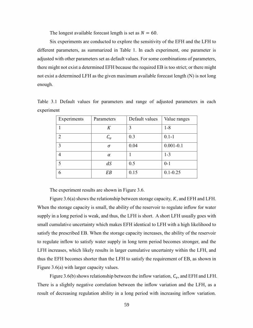
59
The longest available forecast length is set as 𝑁 = 60.
Six experiments are conducted to explore the sensitivity of the EFH and the LFH to
different parameters, as summarized in Table 1. In each experiment, one parameter is
adjusted with other parameters set as default values. For some combinations of parameters,
there might not exist a determined EFH because the required EB is too strict; or there might
not exist a determined LFH as the given maximum available forecast length (N) is not long
enough.
Table 3.1 Default values for parameters and range of adjusted parameters in each
experiment
Experiments Parameters Default values Value ranges
1 𝐾 3 1-8
2 𝐶𝑣 0.3 0.1-1
3 𝜎 0.04 0.001-0.1
4 𝛼 1 1-3
5 𝑑𝑆 0.5 0-1
6 𝐸𝐵 0.15 0.1-0.25
The experiment results are shown in Figure 3.6.
Figure 3.6(a) shows the relationship between storage capacity, 𝐾, and EFH and LFH.
When the storage capacity is small, the ability of the reservoir to regulate inflow for water
supply in a long period is weak, and thus, the LFH is short. A short LFH usually goes with
small cumulative uncertainty which makes EFH identical to LFH with a high likelihood to
satisfy the prescribed EB. When the storage capacity increases, the ability of the reservoir
to regulate inflow to satisfy water supply in long term period becomes stronger, and the
LFH increases, which likely results in larger cumulative uncertainty within the LFH, and
thus the EFH becomes shorter than the LFH to satisfy the requirement of EB, as shown in
Figure 3.6(a) with larger capacity values.
Figure 3.6(b) shows relationship between the inflow variation, 𝐶𝑣, and EFH and LFH.
There is a slightly negative correlation between the inflow variation and the LFH, as a
result of decreasing regulation ability in a long period with increasing inflow variation.

60
When the inflow variation is large (equivalent the case that the reservoir capacity is small),
the LFH is small, and consequently there is higher chance for the EFH identical to the LFH,
as the cumulative uncertainty at the LFH might be small enough to satisfy the given EB.
When the inflow variation is small, the LFH is large, and consequently, the cumulative
uncertainty at the LFH is too large to satisfy the given EB, thus, the EFH is shorter than
the LFH and depends on the estimates of the ending storage. However, as shown in Figure
3.6(b), when the inflow variation is small (i.e., most stable inflow), a determined EFH
rarely exists with the given EB and ending storage. This can be explained as below: more
stable inflow corresponds to a longer LFH, which is likely associated with higher forecast
uncertainty and thus a larger EB is needed to make the error involved in release decision
satisfy the EB.
Figure 3.6(c) shows the relationship between the forecast uncertainty level,𝜎, and
EFH and LFH. With increasing forecast uncertainty level, the EFH decreases quickly, and
no determined EFH exists when the forecast uncertainly level is high, which is a direct
result of increasing uncertainty. The relationship between the LFH and the forecast
uncertainty level, 𝜎, also depends on how uncertainty changes with the forecast lead time.
If the uncertainty level increases rapidly with the forecast lead time, then a shorter LFH
will be preferred. In Figure 3.6(c), when the uncertainty level, 𝜎 , is relatively small,
increasing 𝜎 makes the uncertainty increases faster with forecast lead time, thus, will
decreases the LFH, i.e., there will be a preference on short term forecast with less
uncertainty. But due to the fact that we limit the forecast uncertainty no larger than the
inflow variation when the uncertainty is large, when the uncertainty level, 𝜎, is large, the
uncertainty will become stable soon after the first few stages, and, there will be no longer
a preference for short LFH.
Figure 3.6(d) shows the relationship between demand variation, 𝛼, and EFH and
LFH. Increasing the fluctuation of demand is similar to increasing the variation of inflow.
Thus, in general, the LFH decreases with increasing demand variation, and thus the chance
for the EFH to be identical to the LFH will be higher as the cumulative uncertainty within
the LFH becomes smaller. This figure also shows a slightly positive relationship between
𝛼 and the EFH, which is caused by setting that the first six stages as a low demand period
in the case study, i.e., the increasing of 𝛼 will decrease the absolute value of the release at

61
the first stage, and thus, make it easier to satisfy the given EB, which is an absolute error.
Figure 6(e) shows the relationship between the uncertainty of the ending storage
estimate, 𝑑𝑆, and EFH and LFH. By definition, the LFH is irrelevant to the ending storage
estimate. As shown in the figure, a determined EFH exists with a higher possibility with a
smaller ending storage estimation uncertainty, as it will allow higher inflow uncertainty
with a given error bound. However, the benefit of decreasing the ending storage estimation
uncertainty is not apparent, as the cumulated inflow uncertainty is dominant unless the
inflow uncertainty is very small.
Finally, Figure 6(f) shows the relationship between 𝐸𝐵 and EFH and LFH. By
definition, the LFH is irrelevant to a given error bound. It is clear that a larger EB will lead
to a larger EFH as it will allow higher inflow uncertainty.
(a) Experiment 1: relationship between 𝐾 and the EFH and the LFH
Figure 3.6 Results of six experiments

62
Figure 3.6 (cont.)
(b) Experiment 2: relationship between 𝐶𝑣 and the EFH and the LFH
(c) Experiment 3: relationship between 𝜎 and the EFH and the LFH

63
Figure 3.6 (cont.)
(d) Experiment 4: relationship between 𝛼 and the EFH and the LFH
(e) Experiment 5: relationship between 𝑑𝑆 and the EFH and the LFH

64
Figure 3.6 (cont.)
(f) 6: relationship between 𝐸𝐵 and the EFH and the LFH
3.5 Conclusions
This study continues the efforts to determine the effective forecast horizon. A multi-
stage reservoir operation model is first set up for a single reservoir with single a demand
site, and the properties of the optimal solution, e.g. the relationships of MU and the tangent
relationship between the cumulative release curve and the cumulative inflow curve, are
analyzed, and the influence of forecast uncertainty on release decision is discussed. For a
given cumulative inflow forecast, 𝐼1, 𝐼2, … , 𝐼𝑁, characterized with inflow uncertainty time
series under certain confidence levels, such as [𝐼1, 𝐼1̅], [𝐼2, 𝐼2̅], … , [𝐼𝑁 , 𝐼�̅�], and the estimate
of ending storage, [𝑆𝑁 , 𝑆𝑁̅̅ ̅], the most optimistic scenario with the lower bound of ending
storage, 𝑆𝑁, will provide the largest amount of release, �̅�1∗, at current stage. Meanwhile, the

65
most pessimistic scenario with the upper bound of ending storage, 𝑆𝑁̅̅ ̅ will provide the
smallest amount of release,𝑅1∗, at the current stage.
To provide an upper bound for the EFH candidates, the concept of the longest
forecast horizon (LFH), beyond which the future inflow information and associated
uncertainty will no longer affect the error involved in the release decision at the current
stage, is proposed. Correspondingly, the criteria for determining the LFH and the EFH are
further developed. If the LFH satisfies the criterion for EFH, then the EFH is identical to
the LFH; otherwise, the EFH is shorter than the LFH and it is conditioned with a given
storage at the end of the EFH. Based on these criteria, procedures for determining the EFH
are proposed.
Finally, a case study is conducted with synthesized inflow time series. The case study
shows how EFH and LFH are affected by the storage capacity, the inflow variation, the
forecast uncertainty level, the demand variation, the uncertainty of the ending storage
estimates, and the given error bound. It is shown that the LFH has a positive relationship
with storage capacity, negative relationship with inflow variation and demand variation,
and no obvious relationship with the uncertainty of the ending storage estimates and the
given error bound. The relationship between the LFH and the forecast uncertainty level
depends on the characteristics of the inflow forecast uncertainty. Results show that the EFH
has slight negative relationship with the uncertainty of the ending storage estimation, strong
negative relationship with the forecast uncertainty level and strong positive relationship
with the given error bound, and the EFH is more probable to exist under conditions where
a short LFH exist.

66
CHAPTER 4: DECISION SUPPORT TOOL
DEVELOPMENT
A prototype decision support tool for reservoir operation based on analytically
derived reservoir operation rules (or empirical rules) is developed in this section. The
prototype tool provides a web interface for users to upload data, select operation rules, and
view results. This work in this chapter shows how to apply analytically derived reservoir
operation rules to guide real-world reservoir operation.
4.1 System Design
This prototype decision support system provides the following functions, including
those for authenticating system, defining reservoirs, uploading data, selecting analytical
reservoir operation rules from the database, and displaying results. The detailed description
of each function is described as follows:
(1) Authentication: users need to login to the system to set up reservoirs, manage reservoir
data, select rules, and view results.
(2) Reservoir definition: the system assigns a unique ID for the reservoir, which will be
used to identify the reservoir in the database system to link the properties, data, and the
results to the reservoir. Then, the system will require some key properties of the reservoir
(system) from users as inputs, e.g., reservoir system type (single reservoir, system of
reservoirs in parallel, system of reservoirs in cascade), reservoir purpose (water supply,
energy production, flood control, etc.)
(3) Date upload: upload the data of the reservoir (system) to the decision support system.
The system is designed to handle both single values and time series data. Single value data,
such as the number of reservoirs in the system, the number of stages, is input directly from
the interface and saved in the database, and time series data, such as the demands over
stages, the inflow over stages, is uploaded as files, and the database system is used to store
the location of the file.

67
(4) Rule selection: the system provides users a list of analytical rules matching the
properties of the reservoir (system), and provides a list of necessary data required by each
rule. For example, for a single reservoir for water supply purpose, the system will match a
list of reservoir operation rules, such as calculating the optimal release decisions, providing
the effective forecast horizon (EFH) and longest forecast horizon (LFH), etc. Users can
select a rule from the system to be applied to the reservoir after necessary data being
uploaded. Once an analytical rule is selected, the system will prepare input files for the
corresponding program of the rule, and execute the program.
(6) Result display: the results by each of the programs will be displayed via figures, tables,
and text.
Figure 4.1 provides a flow chart for using the prototype decision support system,
showing the procedures to use the functions described above.
Start
Define a reservoir
Upload available data
Provide a list of analytical reservoir
operation rules suitable for the reservoir
Upload necessary data and select a rule
Execute the rule and display results
End
Figure 4.1 Flow chart for applying an analytical rule
4.2 An Illustrative Case
In this section, an illustrative case is provided to show the procedures of using the
prototype decision support system. As an example, the optimal release decisions for a

68
single water supply reservoir are provided based on the analytical results, i.e., the reservoir
is empty when the marginal utility (MU) decreases, and full when the MU increases; and,
otherwise, the MU is constant over stages.
First, we login the system, and the web-based homepage is shown as Figure 4.2.
Figure 4.2 The webpage of the decision support tool
Then, a single reservoir system for water supply purpose is set up as shown in Figure
4.3 and data is uploaded as shown in Figure 4.4.

69
Figure 4.3 Setting up a water supply reservoir
Figure 4.4. Uploading data
After proceeding to the rule list (as shown in Figure 4.5), a proper rule is selected
(the rule shown in Figure 4.5 with Rule ID 1), and the result of the rule is visualized as
shown in Figure 4.6, which shows the optimal release decision and storage at each stage.

70
Figure 4.5 Choosing analytical rules available for a single water supply reservoir
Figure 4.6 Visualizing results
4.3 Summary
In this section, a prototype reservoir operation decision support system based on
analytical reservoir operation rules is developed. This system provides a web interface for

71
users to set up reservoirs, upload data, and provide a list of applicable analytical reservoir
operation rules based on the inputs from the user. After running the program, the user can
view the results.
This prototype system shows the potential of applying analytical reservoir operation
rules for practical purposes. Though the analytically derived reservoir operation rules can
be limited due to simplifications and assumptions required by the analysis, the derived rules
are mostly generic; furthermore, the generic rules can be used for designing
computationally effective algorithms. The development of a decision support system
provides an implementation of the theoretically derived or empirical rules directly for
guiding real-world reservoir operations.
The current system can be used to provide optimal release decisions for single
reservoir, optimal release decisions for system of reservoirs in parallel, as well as effective
forecast horizons for single reservoir operation under uncertain forecast. The system also
provides a flexible framework for additional analytical rules to be added to the system. For
an analytical reservoir operation rule that is not included in the system, as long as the
program of the rule is developed following some simple requirements on the input and
output file formats, the rule can be added to the system by simply uploading the program
to the server and updating relevant information in the database. Thus, with the capability
of adding more rules, the system can be updated to solve various reservoir operation issues.
72
CHAPTER 5: CONCLUSIONS
This study applies an analytical approach based on the Karush–Kuhn–Tucker (KKT)
conditions, to solve reservoir operation problems, in particular, to establish procedures to
determine the effective forecast horizon (EFH) and to develop an algorithm to solve the
optimal solution for a system of multiple reservoirs in parallel. In addition, a prototype
reservoir operation decision support system is developed to demonstrate the use of the
analytical results to practical problems.
In the Chapter 2, a multi-stage optimization model is set up to derive the properties
of optimal release decisions for a system of reservoir in parallel with a single demand site,
and an algorithm is further developed based on the analytical results to solve for the optimal
solution for such a system. Through the analytical derivation, we first identify feasible
combinations of the release conditions, storage conditions and the marginal utility changes
between two consecutive stages as part of the optimal solution, and further extend the
optimality conditions to the entire study horizon to identify the properties of the optimal
operations for such reservoir systems. Further, based on the understanding of the properties
of the optimal solution, an algorithm is developed to solve parallel reservoir operation
problems, with less computational requirement compared to regular numerical approaches.
A synthetic case study is conducted and shows the effectiveness and validity of the
algorithm. The limitations of this work include the lack of uncertainty considerations and
the generality of the algorithm to be applied to different types of reservoir systems.
However, this work still provides an example of applying analytical results for algorithm
development.
In Chapter 3, to develop procedures to determine the EFH, a multi-stage reservoir
operation model is first set up for a single reservoir with single a demand site, and the
properties of the optimal solution are analyzed. Based on these properties, the influences
of forecast uncertainty on release decisions are discussed, and two special inflow scenarios,
i.e., the most optimistic and pessimistic inflow scenario, are identified to provide the upper
and lower bounds of the optimal release decision at current stage under forecast with
uncertainty. Following this, the concept of the longest forecast horizon (LFH) is proposed

73
as an upper bound for the EFH candidates, and criteria and procedures for determining the
LFH and the EFH are developed. Finally, a synthetic case study is conducted, providing
insights on the influence of various factors to the EFH and the LFH, while validating the
proposed criteria and procedures. Though this work is limited by the assumptions required
by the theoretical model, and the simplified representation of the forecast uncertainty, it
provides a set of practical criteria and procedures to determine the EFH and the LFH. To
further improve the work of this thesis, more analytical work can be done to show the
relationship between EFH, LFH and other factors, and a better representation of forecast
uncertainty, e.g., uncertainty represented as probability distribution, can also help better
understand how the forecast uncertainty affects the optimal release decision.
In Chapter 4, a prototype reservoir operation decision support system is developed
based on the analytical results obtained from this thesis and other related studies. Users can
use a graphical user interface (GUI) to upload data, execute model, and receive information
support for reservoir operation. Though the results might be limited by the assumptions
and formulation of the theoretical model, it provides a new approach to optimize reservoir
operation activities, which is usually not limited by heavy computational requirements as
compared to the numerical approaches used for reservoir operation problems, such as
dynamic programming. This prototype system, though still needing further improvement,
provides a new perspective on how to apply analytical results for practical purposes.
As a summary, this thesis makes efforts on the derivation and application of
analytical results to optimize reservoir operations. In particular, this work focuses on the
following three aspects: using analytical results to develop algorithms, i.e., the algorithm
for parallel reservoir operation problems, using analytical results to prove some properties
of the optimal reservoir operation decisions, i.e., establishing criteria and procedures for
determining EFH and LFH, and developing applications of analytical results for real-world
reservoir operation, i.e., development of the prototype reservoir operation decision support
system. In the future, more work will be needed to explore more possibilities of applying
analytical approaches to addressing the various reservoir operation issues and using
analytical results for practical purposes.

74
REFERENCES
Bazaraa, M.S.; Sherali, H.D.; Shetty, C.M. Nonlinear Programming: Theory and
Algorithms; John Wiley & Sons: Hoboken, NJ, USA, 2013; pp. 188–199.
Bower, B. T., Hufschmidt, M. M., & Reedy, W. W. (1962). Operating procedures: Their
role in the design of water-resource systems by simulation analyses. Design of water
resource systems, 443-458.
Castelletti, A., Galelli, S., Restelli, M., & Soncini‐Sessa, R. (2010). Tree‐based
reinforcement learning for optimal water reservoir operation. Water Resources
Research, 46(9).
Chandramouli, V., & Deka, P. (2005). Neural network based decision support model for
optimal reservoir operation. Water resources management, 19(4), 447-464.
Chang, L. C., & Chang, F. J. (2009). Multi-objective evolutionary algorithm for operating
parallel reservoir system. Journal of hydrology, 377(1), 12-20.
Clark, E. J. (1950). New York control curves. Journal (American Water Works
Association), 42(9), 823-827.
Ding, W., Zhang, C., Peng, Y., Zeng, R., Zhou, H., & Cai, X. (2015). An analytical
framework for flood water conservation considering forecast uncertainty and
acceptable risk. Water Resources Research, 51(6), 4702-4726.
Ding, W., Zhang, C., Cai, X., Li, Y., & Zhou, H. (2017). Multiobjective hedging rules for
flood water conservation. Water Resources Research, 53(3), 1963-1981.
Draper, A. J., & Lund, J. R. (2004). Optimal hedging and carryover storage value. Journal
of Water Resources Planning and Management, 130(1), 83-87.
Hui, R., & Lund, J. R. (2015). Optimal flood pre-releases—flood hedging for a single
reservoir. In World Environmental and Water Resources Congress 2015 (pp. 2192-
2201).
Jairaj, P. G., & Vedula, S. (2003). Modeling reservoir irrigation in uncertain hydrologic
environment. Journal of irrigation and drainage engineering, 129(3), 164-172.
Jalali, M. R., Afshar, A., & Marino, M. A. (2007). Multi-colony ant algorithm for
continuous multi-reservoir operation optimization problem. Water Resources
Management, 21(9), 1429-1447.
Koutsoyiannis, D., Efstratiadis, A., & Karavokiros, G. (2002). A decision support tool for
the management of multi‐reservoir system. JAWRA Journal of the American Water
Resources Association, 38(4), 945-958.
Labadie, J. W. (2004). Optimal operation of multireservoir systems: state-of-the-art
review. Journal of water resources planning and management, 130(2), 93-111.
Lund, J. R., & Guzman, J. (1999). Derived operating rules for reservoirs in series or in
parallel. Journal of Water Resources Planning and Management, 125(3), 143-153.
Mishalani, N. R., & Palmer, R. N. (1988). Forecast uncertainty in water supply reservoir
operation. JAWRA Journal of the American Water Resources Association, 24(6),
1237-1245.
Neelakantan, T. R., & Sasireka, K. (2015). Review of hedging rules applied to reservoir
operation. Int. J. Eng. Technol, 7(5), 1571-1580.
75
Oliveira, R., & Loucks, D. P. (1997). Operating rules for multireservoir systems. Water
resources research, 33(4), 839-852.
Rippl W. The capacity of storage-reservoirs for water-supply. [C]//Minutes of the
Proceedings of the Institution of Civil Engineers. Thomas Telford-ICE Virtual Library,
1883, 71(1883): 270-278.
Shiau, J. T. (2011). Analytical optimal hedging with explicit incorporation of reservoir
release and carryover storage targets. Water resources research, 47(1).
Stedinger, J. R., Sule, B. F., & Loucks, D. P. (1984). Stochastic dynamic programming
models for reservoir operation optimization. Water resources research, 20(11), 1499-
1505.
Thomas, H. A., and Fiering, M. B. (1962). “Mathematical synthesis of streamflow
sequences for the analysis of river basins by simulation.” Design of water resource
systems, Harvard University Press, Cambridge, MA, 459–493.
Wan, W., Zhao, J., Lund, J. R., Zhao, T., Lei, X., & Wang, H. (2016). Optimal Hedging
Rule for Reservoir Refill. Journal of Water Resources Planning and
Management, 142(11), 04016051.
Wurbs, R. A. (1993). Reservoir-system simulation and optimization models. Journal of
water resources planning and management, 119(4), 455-472.
Xu, W., Zhao, J., Zhao, T., & Wang, Z. (2014). Adaptive reservoir operation model
incorporating nonstationary inflow prediction. Journal of Water Resources Planning
and Management, 141(8), 04014099.
Yeh, W. W. G. (1985). Reservoir management and operations models: A state‐of‐the‐art
review. Water resources research, 21(12), 1797-1818.
You, J. Y., & Cai, X. (2008a). Hedging rule for reservoir operations: 1. A theoretical
analysis. Water resources research, 44(1).
You, J. Y., & Cai, X. (2008b). Hedging rule for reservoir operations: 2. A numerical
model. Water resources research, 44(1).
You, J. Y., & Cai, X. (2008c). Determining forecast and decision horizons for reservoir
operations under hedging policies. Water resources research, 44(11).
Wardlaw, R., & Sharif, M. (1999). Evaluation of genetic algorithms for optimal reservoir
system operation. Journal of water resources planning and management, 125(1), 25-
33.
Zeng, X., Hu, T., Xiong, L., Cao, Z., & Xu, C. (2015). Derivation of operation rules for
reservoirs in parallel with joint water demand. Water Resources Research, 51(12),
9539-9563.
Zhao, J., Cai, X., & Wang, Z. (2011). Optimality conditions for a two‐stage reservoir
operation problem. Water Resources Research, 47(8).
Zhao, T., Yang, D., Cai, X., Zhao, J., & Wang, H. (2012). Identifying effective forecast
horizon for real‐time reservoir operation under a limited inflow forecast. Water
Resources Research, 48(1).
Zhao, T., Cai, X., & Yang, D. (2011). Effect of streamflow forecast uncertainty on real-
time reservoir operation. Advances in water resources, 34(4), 495-504.
Zhao, T., Zhao, J., Lund, J. R., & Yang, D. (2014). Optimal hedging rules for reservoir
flood operation from forecast uncertainties. Journal of Water Resources Planning and
Management, 140(12), 04014041.

76
APPENDIX A: DERIVATION
The model is formulated as follows:
Obj. max∑𝑏𝑖 (∑𝑟𝑖,𝑗
𝑀
𝑗=1
)
𝑁
𝑖=1
(𝐴. 1)
𝑠. 𝑡.
𝑠𝑖−1,𝑗 + 𝑖𝑖,𝑗 − 𝑟𝑖,𝑗 = 𝑠𝑖,𝑗 , 𝑓𝑜𝑟 𝑖 = 1, … ,𝑁 𝑎𝑛𝑑 𝑗 = 1,2, … ,𝑀 (𝐴. 2)
𝑠𝑖,𝑗 ≥ 0, 𝑓𝑜𝑟 𝑖 = 1,… , 𝑁 − 1 𝑎𝑛𝑑 𝑗 = 1,2, … ,𝑀 (𝐴. 3)
𝑠𝑖,𝑗 ≤ 𝐾𝑗, 𝑓𝑜𝑟 𝑖 = 1,… , 𝑁 − 1 𝑎𝑛𝑑 𝑗 = 1,2, … ,𝑀 (𝐴. 4)
𝑟𝑖,𝑗 ≥ 0, 𝑓𝑜𝑟 𝑖 = 1,2, … , 𝑁 𝑎𝑛𝑑 𝑗 = 1,2, … ,𝑀 (𝐴. 5)
Here, i is the index of time and j is the index of reservoirs, M is the total number of
reservoirs and N is the total number of stages, 𝑏𝑖(𝑟) is the concave utility function of water
supply at stage i, 𝑠𝑖,𝑗 is the storage of reservoir j at the end of stage i, the initial and ending
storage of reservoir j is given as 𝑠0,𝑗 and 𝑠𝑁,𝑗 respectively, 𝑟𝑖,𝑗 is the release of reservoir j
during stage i, 𝑖𝑖,𝑗 is the inflow to reservoir j during stage i, and 𝐾𝑗 is the storage capacity
of reservoir j.
Transform for applying KKT condition.
Obj. max∑𝑏𝑖 (∑𝑟𝑖,𝑗
𝑀
𝑗=1
)
𝑁
𝑖=1
(𝐴. 6)
𝑠. 𝑡.
𝑠𝑖−1,𝑗 + 𝑖𝑖,𝑗 − 𝑟𝑖,𝑗 − 𝑠𝑖,𝑗 = 0, 𝑓𝑜𝑟 𝑖 = 1,… ,𝑁 𝑎𝑛𝑑 𝑗 = 1,2, … ,𝑀 (𝐴. 7)
−𝑠𝑖,𝑗 ≤ 0, 𝑓𝑜𝑟 𝑖 = 1,… , 𝑁 − 1 𝑎𝑛𝑑 𝑗 = 1,2, … ,𝑀 (𝐴. 8)
𝑠𝑖,𝑗 ≤ 𝐾𝑗, 𝑓𝑜𝑟 𝑖 = 1,… , 𝑁 − 1 𝑎𝑛𝑑 𝑗 = 1,2, … ,𝑀 (𝐴. 9)
−𝑟𝑖,𝑗 ≤ 0, 𝑓𝑜𝑟 𝑖 = 1,2, … , 𝑁 𝑎𝑛𝑑 𝑗 = 1,2, … ,𝑀 (𝐴. 10)
Apply KKT condition.

77
−𝜕
𝜕𝑟𝐼𝐽∑𝑏𝑖 (∑𝑟𝑖,𝑗
𝑀
𝑗=1
)
𝑁
𝑖=1
+𝜕
𝜕𝑟𝐼𝐽∑∑𝜆𝑏,𝑖,𝑗(𝑠𝑖,𝑗 − 𝑠𝑖−1,𝑗 − 𝑖𝑖,𝑗 + 𝑟𝑖,𝑗)
𝑀
𝑗=1
𝑁
𝑖=1
+𝜕
𝜕𝑟𝐼𝐽∑∑𝜆𝑒,𝑖,𝑗(−𝑠𝑖,𝑗)
𝑀
𝑗=1
𝑁−1
𝑖=1
+𝜕
𝜕𝑟𝐼𝐽∑∑𝜆𝑓,𝑖,𝑗(𝑠𝑖,𝑗 − 𝐾𝑗)
𝑀
𝑗=1
𝑁−1
𝑖=1
+𝜕
𝜕𝑟𝐼𝐽∑∑𝜆𝑟,𝑖,𝑗(−𝑟𝑖,𝑗)
𝑀
𝑗=1
𝑁
𝑖=1
= 0,
𝑓𝑜𝑟 𝐼 = 1,2, … ,𝑁, 𝐽 = 1,2, … ,𝑀 (𝐴. 11)
−𝜕
𝜕𝑠𝐼𝐽∑𝑏𝑖 (∑𝑟𝑖,𝑗
𝑀
𝑗=1
)
𝑁
𝑖=1
+𝜕
𝜕𝑠𝐼𝐽∑∑𝜆𝑏,𝑖,𝑗(𝑠𝑖,𝑗 − 𝑠𝑖−1,𝑗 − 𝑖𝑖,𝑗 + 𝑟𝑖,𝑗)
𝑀
𝑗=1
𝑁
𝑖=1
+𝜕
𝜕𝑠𝐼𝐽∑∑𝜆𝑒,𝑖,𝑗(−𝑠𝑖)
𝑀
𝑗=1
𝑁−1
𝑖=1
+𝜕
𝜕𝑠𝐼𝐽∑∑𝜆𝑓,𝑖,𝑗(𝑠𝑖 − 𝐾𝑗)
𝑀
𝑗=1
𝑁−1
𝑖=1
+𝜕
𝜕𝑠𝐼𝐽∑∑𝜆𝑟,𝑖,𝑗(−𝑟𝑖,𝑗)
𝑀
𝑗=1
𝑁
𝑖=1
= 0,
𝑓𝑜𝑟 𝐼 = 1,… ,𝑁 − 1 𝑎𝑛𝑑 𝐽 = 1,2, … ,𝑀 (𝐴. 12)
−𝑠𝑖,𝑗 ≤ 0, 𝑓𝑜𝑟 𝑖 = 1,… ,𝑁 − 1 𝑎𝑛𝑑 𝑗 = 1,2, … ,𝑀 (𝐴. 13)
𝑠𝑖,𝑗 ≤ 𝐾𝑖 , 𝑓𝑜𝑟 𝑖 = 1,… ,𝑁 − 1 𝑎𝑛𝑑 𝑗 = 1,2, … ,𝑀 (𝐴. 14)
𝜆𝑒,𝑖,𝑗𝑠𝑖,𝑗 = 0, 𝑓𝑜𝑟 𝑖 = 1,… ,𝑁 − 1 𝑎𝑛𝑑 𝑗 = 1,2, … ,𝑀 (𝐴. 15)
𝜆𝑓,𝑖,𝑗(𝑠𝑖,𝑗 − 𝐾𝑖) = 0, 𝑓𝑜𝑟 𝑖 = 1,… ,𝑁 − 1 𝑎𝑛𝑑 𝑗 = 1,2, … ,𝑀 (𝐴. 16)
𝜆𝑟,𝑖,𝑗𝑟𝑖,𝑗 = 0, 𝑓𝑜𝑟 𝑖 = 1,… ,𝑁 𝑎𝑛𝑑 𝑗 = 1,2, … ,𝑀 (𝐴. 17)
𝜆𝑒,𝑖,𝑗 ≥ 0, 𝑓𝑜𝑟 𝑖 = 1,… ,𝑁 − 1 𝑎𝑛𝑑 𝑗 = 1,2, … ,𝑀 (𝐴. 18)
𝜆𝑓,𝑖,𝑗 ≥ 0, 𝑓𝑜𝑟 𝑖 = 1,… ,𝑁 − 1 𝑎𝑛𝑑 𝑗 = 1,2, … ,𝑀 (𝐴. 19)
𝜆𝑟,𝑖,𝑗 ≥ 0, 𝑓𝑜𝑟 𝑖 = 1,2, … ,𝑁 𝑎𝑛𝑑 𝑗 = 1,2, … ,𝑀 (𝐴. 20)
Here, 𝜆𝑏,𝑖,𝑗 is the shadow price for the mass balance constrain, Eq. (A.2), of reservoir j at
stage i, 𝜆𝑒,𝑖,𝑗 is the shadow price for non-negative storage constraints, Eq. (A.3), of
reservoir j at the end of stage i, 𝜆𝑓,𝑖,𝑗 is the shadow price for storage capacity constraints,
Eq. (A.4), of reservoir j at the end of stage i, and 𝜆𝑟,𝑖,𝑗 is the shadow price for non-negative

78
release constraints, Eq. (A.5), of reservoir j on stage i. Eq. (A.21) – Eq. (A.22) could be
obtained by simplifying Eq. (A.12) – Eq. (A.20).
𝜆𝑏,𝑖,𝑗 = 𝑏𝑖′ (∑𝑟𝑖,𝑗
𝑀
𝑗=1
) + 𝜆𝑟,𝑖,𝑗, 𝑓𝑜𝑟 𝑖 = 1,2, … ,𝑁 𝑎𝑛𝑑 𝑗 = 1,2, … ,𝑀 (𝐴. 21)
𝜆𝑏,𝑖+1,𝑗 + 𝜆𝑒,𝑖,𝑗 − 𝜆𝑓,𝑖,𝑗 = 𝜆𝑏,𝑖,𝑗, 𝑓𝑜𝑟 𝑖 = 1,2, … ,𝑁 − 1 𝑎𝑛𝑑 𝑗 = 1,2, … ,𝑀 (𝐴. 22)
Substitute Eq. (A.21) to Eq. (A.22),
𝑏𝑖+1′ (∑𝑟𝑖+1,𝑗
𝑀
𝑗=1
) + 𝜆𝑟,𝑖+1,𝑗 + 𝜆𝑒,𝑖,𝑗 − 𝜆𝑒,𝑖,𝑗 = 𝑏𝑖′ (∑𝑟𝑖,𝑗
𝑀
𝑗=1
) + 𝜆𝑟,𝑖,𝑗 ,
𝑓𝑜𝑟 𝑖 = 1,2, … ,𝑁 − 1 𝑎𝑛𝑑 𝑗 = 1,2, … ,𝑀 (𝐴. 23)
𝑏𝑖+1′ (∑𝑟𝑖+1,𝑗
𝑀
𝑗=1
) + 𝜆𝑒,𝑖,𝑗 − 𝜆𝑓,𝑖,𝑗 = 𝑏𝑖′ (∑𝑟𝑖,𝑗
𝑀
𝑗=1
) + (𝜆𝑟,𝑖,𝑗 − 𝜆𝑟,𝑖+1,𝑗),
𝑓𝑜𝑟 𝑖 = 1,2, … ,𝑁 − 1 𝑎𝑛𝑑 𝑗 = 1,2, … ,𝑀 (𝐴. 24)

79
APPENDIX B: PROOF
If we solve the optimization problem under the assumption (Assumption I) that all
reservoirs will release as much water as possible before a MU decrease without considering
future droughts, i.e., all reservoirs storages achieve the lowest possible value when MU
decreases, we will obtain a result more conservative for current stages. Thus, as shown in
Figure B.1, in the optimal solution solved under Assumption I, there is no water saved from
earlier stages with high MU, e.g., stages of Piece 1 and Piece 2, to later stages with high
MU, e.g., stages of Piece 4, while in the optimal solution of the original problem that is not
subject to Assumption I, some water can might be saved from earlier stages with high MU
to later stages with high MU. To obtain the optimal solution of the original problem from
the optimal solution solved under Assumption I, instead of releasing all available water
before MU decreases, e.g., at stages of Piece 1 and Piece 2, some reservoirs might not be
empty when MU decreases and some water might be saved to later stages with high MU,
e.g., stages of Piece 4, if the MU is higher at later stages than that of the earlier stages. The
maximum amount of water saved is constrained by the excessive storage capacity of the
reservoirs after storing as much water as possible during the stages with low MU, e.g.
stages of Piece 3 in Figure B.1.
We will focus on the first occurrence of MU increase in the optimal solution solved
under Assumption I. Under the following four situations, the relationship between the
optimal solution solved for the original problem that is not subject to Assumption I and the
optimal solution solved under Assumption I are discussed.

80
(1) Optimal Solution Under Assumption I
Marg
inal U
tility
Piece 2
Piece 3
Piece 4
Piece 1Empty
No water saved from 1,2 to 4
(2) Optimal Solution of the Original Problem (Not Subject to
Assumption I)
Marg
inal U
tility
Piece 2
Piece 3
Piece 4
Piece 1
Not Sure Empty or Not
Possible water saved from 1,2 to 4
Not Sure whether 1,2 and 4 are single
piece or not
Figure B.1 Illustration of the optimal solutions solved with/without Assumption I
(1) Assume all reservoirs become full at the first occurrence of MU increase in the
study horizon with the optimal solution solved under Assumption I. By removing
Assumption I from the optimal solution solved under Assumption I, no more water can be
saved from stages of Piece 1 & 2 to stages of Piece 4, as the storages are already full at the
end of Piece 3. It is possible that there will be water saved from Piece 4 to the future, which
will possibly make the MU of Piece 4 higher, and thus, MU of Piece 4 is still higher than
that of Piece 3, which means reservoirs will still be full at the end of Piece 3 after removing
Assumption I. Thus, if all reservoirs become full at the first occurrence of MU increase in
the study horizon with the optimal solution solved with Assumption I, the optimal release
decision before the reservoirs are full solved with Assumption I will not be subject to
Assumption I.
(2) Assume that in the optimal decisions solved with Assumption I, there is no
decrease of MU before the first occurrence of MU increase (i.e., there is a single MU before
the first occurrence of the MU increase) (Piece 1 & 2 in Figure B.1 not exist). By removing
Assumption I from the optimal solution solved under Assumption I, there might be more
water saved from Piece 4 to the future, which will possibly make the MU of Piece 4 higher,
and thus, MU of Piece 4 is still higher than that of Piece 3, thus, reservoirs should save as
much water as possible during stages of Piece 3, which is the same as the optimal solution

81
solved under Assumption I. Thus, if in the optimal decisions solved with Assumption I,
there is no decrease of MU before the first occurrence of MU increase (i.e., there is a single
MU before the first occurrence of the MU increase), then, the optimal release decision
before the first occurrence of MU increase will be the same as the optimal release decision
of the original problem that is not subject to Assumption I.
(3) Assume that no MU increase occurs in the study horizon in the optimal release
decision solved with Assumption I (Piece 4 in Figure B.1 does not exist). Therefore, the
MU keeps decreasing within the study horizon, thus, by removing Assumption I from the
optimal solution solved under Assumption I, there is no need to save water from any piece
to the future, as the MU at any stage is higher than all future stages in the study horizon.
Thus, if no states with increasing MU occurs in the optimal release decision solved with
Assumption I, then the optimal release decision will be the same as the optimal decision of
the original problem that is not subject to Assumption I.
(4) Assume, none of (1), (2) or (3) is satisfied in the optimal release decision under
Assumption I. By removing Assumption I from the optimal solution solved under
Assumption I, it is possible that there is some water saved from Piece 1 & 2 to the future
after Piece 3, e.g., Piece 4. After this reallocation, the MU of Piece 1, 2 and Piece 4 will
still be greater or equal to the lowest MU of these three pieces under the optimal solution
solved under Assumption I, and thus, is still greater than the MU of Piece 3. The reason is
given as follows. The MUs of Piece 1 & 2 have already reached a minimum possible value
in the optimal solution solved under Assumption I, as all reservoir storages are the lowest
possible storage when MU decreases, thus, the MU of Piece 1 & 2 cannot be lower than
that of Piece 3 by removing Assumption I. After removing Assumption I, if the MU of
Piece 4 becomes lower by receiving some water from Piece 1 & 2, then, it cannot be lower
than the lower one of the MUs of Piece 1 & 2 to achieve optimality, thus, is still higher
than that of Piece 3. For reservoirs not full at the end of Piece 3 and not releasing on Piece

82
3 under the optimal solution solved with Assumption I, it is possible for them to save water
from stages of Piece 1 & 2 to stages after Piece 3 under the optimal decision of the original
problem that is not subject to Assumption I, thus, might be not empty at the end of Piece
2. However, there is still no release from such reservoirs during stages of Piece 3, as the
reservoir is not empty when the MU decreases at the end of Piece 2. Thus, after removing
Assumption I, the release decision of Piece 3 will not be changed, though the storage of
the reservoirs during stages of Piece 3 might be different. For other reservoirs, under the
optimal release decision solved with Assumption I, they are already full at the end of Piece
3, thus, it is not possible for them to be not empty at the end of Piece 2 to save water for
the future after removing Assumption I. Thus, if neither the condition of (1), (2) nor (3) are
satisfied in the optimal release decision under Assumption I, then the optimal release
decision between the first occurrence of the MU increase and the adjacent previous
occurrence of the decrease of the MU will be the same as the optimal release decision of
the original problem that is not subject to Assumption I.

83
APPENDIX C: DERIVATION
Formulation:
Obj. max∑𝑏𝑖(𝑟𝑖) (𝐶. 1)
𝑠. 𝑡.
𝑠𝑖−1 + 𝐼𝑖 − 𝑟𝑖 = 𝑠𝑖, 𝑓𝑜𝑟 𝑖 = 1,2, … ,𝑁 (C. 2)
𝑠𝑖 ≥ 0, 𝑓𝑜𝑟 𝑖 = 1,2, … ,𝑁 − 1 (C. 3)
𝑠𝑖 ≤ 𝐾, 𝑓𝑜𝑟 𝑖 = 1,2, … ,𝑁 − 1 (C. 4)
where 𝑏𝑖(𝑟𝑖) is the concave utility function for stage i, 𝑠𝑖 is the storge of reservoir at the
end of stage i, 𝐼𝑖 is the inflow forecast during stage i, 𝑟𝑖 is the release during stage i, K is
the capacity of the reservoir and N is the attempted forecast horizon.
Using KKT condition, the optimization problem could be transformed as follows.
Obj. min −∑𝑏𝑖(𝑟𝑖) (𝐶. 5)
𝑠. 𝑡.
𝑠𝑖−1 + 𝑖𝑖 − 𝑟𝑖 = 𝑠𝑖, 𝑓𝑜𝑟 𝑖 = 1,2, … ,𝑁 (𝐶. 6)
−𝑠𝑖 ≤ 0, 𝑓𝑜𝑟 𝑖 = 1,… ,𝑁 − 1 (𝐶. 7)
𝑠𝑖 ≤ 𝐾, 𝑓𝑜𝑟 𝑖 = 1,… ,𝑁 − 1 (𝐶. 8)
The necessary condition for optimal solution is given as follows.
−𝜕
𝜕𝑟𝐼∑𝑏𝑖(𝑟𝑖)
𝑁
𝑖=1
+∑𝜆𝑏,𝑖𝜕
𝜕𝑟𝐼
𝑁
𝑖=1
(𝑠𝑖 − 𝑠𝑖−1 − 𝑖𝑖 + 𝑟𝑖) + ∑ 𝜆𝑒,𝑖
𝑁−1
𝑖=1
𝜕
𝜕𝑟𝐼(−𝑠𝑖)
+ ∑ 𝜆𝑓,𝑖
𝑁−1
𝑖=1
𝜕
𝜕𝑟𝐼(𝑠𝑖 −𝐾) = 0, 𝑓𝑜𝑟 𝐼 = 1,2, … ,𝑁 (𝐶. 9)

84
−𝜕
𝜕𝑠𝐼∑𝑏𝑖(𝑟𝑖)
𝑁
𝑖=1
+∑𝜆𝑏,𝑖𝜕
𝜕𝑠𝐼
𝑁
𝑖=1
(𝑠𝑖 − 𝑠𝑖−1 − 𝑖𝑖 + 𝑟𝑖) + ∑ 𝜆𝑒,𝑖
𝑁−1
𝑖=1
𝜕
𝜕𝑠𝐼(−𝑠𝑖)
+ ∑ 𝜆𝑓,𝑖
𝑁−1
𝑖=1
𝜕
𝜕𝑠𝐼(𝑠𝑖 − 𝐾) = 0, 𝑓𝑜𝑟 𝐼 = 1,… ,𝑁 − 1 (𝐶. 10)
−𝑠𝑖 ≤ 0, 𝑓𝑜𝑟 𝑖 = 1,… ,𝑁 − 1 (𝐶. 11)
𝑠𝑖 ≤ 𝐾, 𝑓𝑜𝑟 𝑖 = 1,… ,𝑁 − 1 (𝐶. 12)
𝜆𝑒,𝑖𝑠𝑖 = 0, 𝑓𝑜𝑟 𝑖 = 1,… ,𝑁 − 1 (𝐶. 13)
𝜆𝑓,𝑖(𝑠𝑖 − 𝐾) = 0, 𝑓𝑜𝑟 𝑖 = 1, … , 𝑁 − 1 (𝐶. 14)
𝜆𝑒,𝑖 ≥ 0, 𝑓𝑜𝑟 𝑖 = 1,… ,𝑁 − 1 (𝐶. 15)
𝜆𝑓,𝑖 ≥ 0, 𝑓𝑜𝑟 𝑖 = 1,… ,𝑁 − 1 (𝐶. 16)
where 𝜆𝑒,𝑖 is the shadow price for non-negative storage constraints at stage i, 𝜆𝑓,𝑖 is the
shadow price for the capacity constraint at stage i and 𝜆𝑏,𝑖 is the shadow price for the mass
balance constraint at stage i.
From Eq. (C.9) we can have
−𝜕𝑏𝑖(𝑟𝑖)
𝜕𝑟𝑖+ 𝜆𝑏,𝑖 = 0, 𝑓𝑜𝑟 𝑖 = 1,2, … ,𝑁 (𝐶. 17)
From Eq. (C.10) we can have
𝜆𝑏,𝑖−1 − 𝜆𝑏,𝑖 − 𝜆𝑒,𝑖 + 𝜆𝑓,𝑖 = 0, 𝑓𝑜𝑟 𝑖 = 1,… ,𝑁 − 1 (𝐶. 18)

85
APPENDIX D: PROOF
Time (Stages)
Cu
mu
lati
ve I
nfl
ow
/Rele
ase
Cumulative InflowCumulative Release
Legend
Marg
inal
Uti
lity
Marginal UtilityExtension of Piece I
Piece I
Marginal Utility of Extension of Piece I
Sn
S0
Figure D.1 Illustration of MU changes under optimal release decisions
First, we show that the cumulative release curve will be tangent to the cumulative
inflow curve when an empty state occurs. As shown in the Figure D.1, if the intersection
of these two curves are not tangent to each other, i.e., the intersection point is a cross-over
point. Then, if by extending Piece I of the cumulative delivery curve with identical MU
(the extended part is shown as dotted blue line), there is a time period, during which the
extended delivery curve with the same MU as Piece I is above the actual cumulative inflow
curve, and thus, is above the actual cumulative water delivery curve. This means during
this period, the actual MU is higher than the MU of Piece I. Then this contradicts with the
relationship derived for stages with non-negative storage constraint binding, i.e.,
𝑏𝑖′(𝑟𝑖
∗) = 𝑏𝑖+1′ (𝑟𝑖+1
∗ ) + 𝜆𝑒,𝑖 (𝐷. 1)
Thus, if the point is a point of cross-over, this relationship shown in Eq. (D.1) will be
violated.

86
Same derivation can be done for a stage with binding storage capacity constraint. It
could be shown that if the intersection of these two curves are not tangent to each other,
namely, the intersection point is a cross-over point. Then, there is a time period, during
which the actual MU is lower than the MU of the periods before the stage with binding
storage capacity constraint. Then this contradicts with the relationship derived for stages
with storage capacity constraint binding, i.e.,
𝑏𝑖−1′ (𝑟𝑖−1
∗ ) = 𝑏𝑖′(𝑟𝑖
∗) − 𝜆𝑓,𝑖 (𝐷. 2)
Thus, if the point is a point of cross-over, this relationship shown in Eq. (D.2) will be
violated.

87
APPENDIX E: PROOF
Under Case 4 (the non-negative storage constraint becomes binding for the first time
after the initial storage, and then the storage capacity constraint becomes binding at a later
stage), two scenarios, i.e. future water abundant scenario and future water stress scenario,
are discussed.
Figure E.1 shows future water abundant scenario, when more water should be
released in 𝑇𝑓. As shown in the figure, even if more water will be released during 𝑇𝑓, only
release beyond 𝑇𝑑 will be increased. The reservoir is empty at 𝑇𝑑 ,and thus, the release
before 𝑇𝑑 has already reached a maximum. Otherwise, if the release within 𝑇𝑑is increased,
the cumulative water delivery curve will no longer be tangent with the cumulative inflow
curve at 𝑇𝑑 , which contradicts with the optimal solution solved from the optimization
model. Therefore, even if there is more inflow in the future beyond 𝑇𝑓, the decision in 𝑇𝑑
will not be changed.
Time (Stages)
Cu
mu
lati
ve I
nfl
ow
/Rele
ase
Marg
inal
Uti
lity
Cumulative InflowCumulative Release
Legend
Marginal UtilityCumulative Inflow-K
Release if Future Water Abundant
𝑇𝑑
𝑇𝑓
S0
K
Figure E.1 Water Abundant Future
The other scenario is drought in the future. For this situation, as the storage at 𝑇𝑓 has
already reached the maximum, no more water can be saved before 𝑇𝑓. As shown in Figure

88
E.2, if reduce release before 𝑇𝑓, the cumulative water delivery will decrease at 𝑇𝑓, and thus
the cumulative water delivery curve and the cumulative inflow curve moved downward by
the storage capacity will cross over with each other, and thus, is not the optimal solution.
Therefore, with drought in the future, the optimal release decision within 𝑇𝑑 remains
unchanged.
Thus, regardless of the inflow condition beyond 𝑇𝑓, the optimal decision will not be
changed in the 𝑇𝑑 given information in 𝑇𝑓.
Time (Stages)
Cu
mu
lati
ve I
nfl
ow
/Rele
ase
Marg
inal
Uti
lity
Cumulative InflowCumulative Release
Legend
Marginal UtilityCumulative Inflow-K
Release with Future Drought
𝑇𝑑
𝑇𝑓
S0
K
Figure E.2 Water Stress Future
Similar analysis can be conducted for Case 5 (the storage capacity constraint
becomes binding for the first time after the initial storage, and then the non-negative
storage constraint becomes binding at a later stage).

89
APPENDIX F: PROOF
In this appendix, the following statement is proved. For a given inflow forecast for
future N stages, 𝐼1, 𝐼2, … , 𝐼𝑁 , and corresponding inflow uncertainty under certain
confidence levels, such as [𝐼1, 𝐼1̅], [𝐼2, 𝐼2̅], … , [𝐼𝑁 , 𝐼�̅�], and an estimation of ending storage,
[𝑆𝑁 , 𝑆𝑁̅̅ ̅] , among all possible inflow scenarios, the most optimistic scenario, i.e.,
𝐼1,𝑜𝑝𝑡, 𝐼2,𝑜𝑝𝑡, … , 𝐼𝑁,𝑜𝑝𝑡 , which has the highest cumulative inflow at all stages over all
possible scenarios, together with the lower bound of ending storage, 𝑆𝑁 , provides the
largest amount of release, �̅�1∗ , at current stage, and the most pessimistic scenario, i.e.,
𝐼1,𝑝𝑒𝑠, 𝐼2,𝑝𝑒𝑠, … , 𝐼𝑁,𝑝𝑒𝑠, which has the lowest cumulative inflow at all stages over all possible
scenarios, together with the upper bound of ending storage, 𝑆𝑁̅̅ ̅, provides the smallest
amount of release, 𝑅1∗, at current stage.
Proof by contradiction is applied here.
Assume that the optimal release decision, 𝑅1′ , solved under inflow forecast,
𝐼1′ , 𝐼2
′ , … , 𝐼𝑁′ , which is different from the most optimistic one, is greater than the optimal
release decision solved under most optimistic forecast, �̅�1∗, i.e.,
∑𝐼𝑖′
𝑡
𝑖=1
≤∑𝐼𝑖,𝑜𝑝𝑡
𝑡
𝑖=1
, ∀𝑡 = 1,2, … ,𝑁 (𝐹. 1)
𝑅1′ > �̅�1
∗ (𝐹. 2)
thus, over the study horizon, N,
∑𝐼𝑖′
𝑁
𝑖=1
≤∑𝐼𝑖,𝑜𝑝𝑡
𝑁
𝑖=1
(𝐹. 3)
and according to the characteristics of utility function 𝑏𝑖(𝑟𝑖),
𝑏1(𝑅1′ ) > 𝑏1(�̅�1
∗) (𝐹. 4)

90
𝑏1′(𝑅1
′ ) < 𝑏1′(�̅�1
∗) (𝐹. 5)
There should exists at least one stage k (and assume k is the first one) satisfying Eq. (F.6)
& Eq. (F.7),
𝑅𝑘′ > �̅�𝑘
∗ (𝐹. 6)
𝑅𝑘+1′ < �̅�𝑘+1
∗ (𝐹. 7)
where �̅�𝑘∗ is the optimal release decision at stage k solved under the most optimistic forecast,
and 𝑅𝑘′ is the optimal release decision at stage k solved under inflow forecast 𝐼1
′ , 𝐼2′ , … , 𝐼𝑁
′ .
Then,
𝑏𝑘′ (𝑅𝑘
′ ) < 𝑏𝑘′ (�̅�𝑘
∗) (𝐹. 8)
𝑏𝑘+1′ (𝑅𝑘+1
′ ) > 𝑏𝑘+1′ (�̅�𝑘+1
∗ ) (𝐹. 9)
otherwise,
∑𝑅𝑖′
𝑁
𝑖=1
>∑�̅�𝑖∗
𝑁
𝑖=1
(𝐹. 10)
∑𝑅𝑖′
𝑁
𝑖=1
+ 𝑆𝑁 − 𝑆0 >∑�̅�𝑖∗
𝑁
𝑖=1
+ 𝑆𝑁 − 𝑆0 (𝐹. 11)
∑𝐼𝑖′
𝑁
𝑖=1
>∑𝐼𝑖,𝑜𝑝𝑡
𝑁
𝑖=1
(𝐹. 12)
which will contradict with Eq. (F.3).
According to Eq. (F.8) & (F.9), there should be following several possibilities. In the
following discussion, for simplicity, the most optimistic scenario will be referred as Case
1 and the other inflow scenario will be referred as Case 2, and 𝑆�̅�, 𝐼𝑖,𝑜𝑝𝑡, �̅�𝑖∗ will be used to
represent storage, inflow and release for Case 1, and 𝑆𝑖′, 𝐼𝑖
′, 𝑅𝑖′ will be used to represent
storage, inflow and release for Case 2.
(1) 𝑏𝑘′ (𝑅𝑘
′ ) = 𝑏𝑘+1′ (𝑅𝑘+1
′ ) and 𝑏𝑘′ (�̅�𝑘
∗) > 𝑏𝑘+1′ (�̅�𝑘+1
∗ ) . Therefore, for Case 1,
according to the analytical solution, there is an empty state between stage k and stage k+1.
Thus,

91
𝑆𝑘+1′ ≥ 𝑆�̅�+1 = 0 (𝐹. 13)
combining the assumption shown by Eq. (F.1),
∑𝐼𝑖′
𝑘
𝑖=1
+ 𝑆0 − 𝑆𝑘+1′ ≤∑𝐼𝑖,𝑜𝑝𝑡
𝑘
𝑖=1
+ 𝑆0 − 𝑆�̅�+1 (𝐹. 14)
∑𝑅𝑖′
𝑘
𝑖=1
≤∑𝑅�̅�
𝑘
𝑖=1
(𝐹. 15)
This contradicts with the assumption that k is the first stage satisfying Eq. (F.6) and Eq.
(F.7).
(2) 𝑏𝑘′ (𝑅𝑘
′ ) < 𝑏𝑘+1′ (𝑅𝑘+1
′ ) and 𝑏𝑘′ (�̅�𝑘
∗) = 𝑏𝑘+1′ (�̅�𝑘+1
∗ ) . Therefore, for Case 2,
according to the analytical solution, there is a full state between stage k and stage k+1. Thus,
𝐾 = 𝑆𝑘+1′ ≥ 𝑆�̅�+1 (𝐹. 16)
which is the same as Eq. (F.13) and contradicts with the assumption that k is the first stage
satisfying Eq. (F.6) and Eq. (F.7).
(3) 𝑏𝑘′ (𝑅𝑘
′ ) < 𝑏𝑘+1′ (𝑅𝑘+1
′ ) and 𝑏𝑘′ (�̅�𝑘
∗) > 𝑏𝑘+1′ (�̅�𝑘+1
∗ ) . Therefore, for Case 1,
according to the analytical solution, there is an empty state between stage k and stage k+1,
and for Case 2, there is a full state between stage k and stage k+1. Thus,
𝐾 = 𝑆𝑘+1′ ≥ 𝑆�̅�+1 = 0 (𝐹. 17)
which is also the same as Eq. (F.13) and contradicts with the assumption that k is the first
stage satisfying Eq. (F.6) and Eq. (F.7).
(4) 𝑏𝑘′ (𝑅𝑘
′ ) < 𝑏𝑘+1′ (𝑅𝑘+1
′ ) and 𝑏𝑘′ (�̅�𝑘
∗) < 𝑏𝑘+1′ (�̅�𝑘+1
∗ ). Therefore, for both Case 1
and Case 2, according to the analytical solution, there is a full state between stage k and
stage k+1. Thus,
𝐾 = 𝑆𝑘+1′ = 𝑆�̅�+1 = 𝐾 (𝐹. 18)
combining the assumption shown by Eq. (F.1),
∑𝐼𝑖′
𝑘
𝑖=1
+ 𝑆0 − 𝑆𝑘+1′ ≤∑𝐼�̅�
𝑘
𝑖=1
+ 𝑆0 − 𝑆�̅�+1 (𝐹. 19)
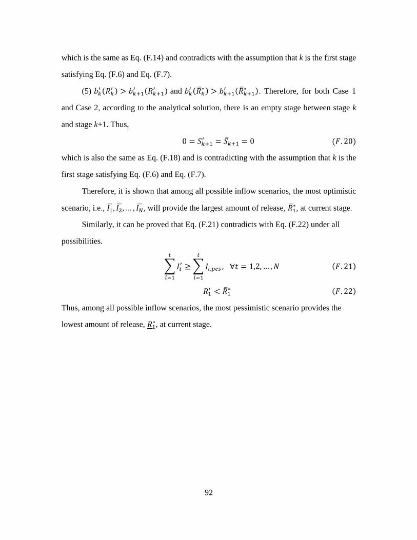
92
which is the same as Eq. (F.14) and contradicts with the assumption that k is the first stage
satisfying Eq. (F.6) and Eq. (F.7).
(5) 𝑏𝑘′ (𝑅𝑘
′ ) > 𝑏𝑘+1′ (𝑅𝑘+1
′ ) and 𝑏𝑘′ (�̅�𝑘
∗) > 𝑏𝑘+1′ (�̅�𝑘+1
∗ ). Therefore, for both Case 1
and Case 2, according to the analytical solution, there is an empty stage between stage k
and stage k+1. Thus,
0 = 𝑆𝑘+1′ = 𝑆�̅�+1 = 0 (𝐹. 20)
which is also the same as Eq. (F.18) and is contradicting with the assumption that k is the
first stage satisfying Eq. (F.6) and Eq. (F.7).
Therefore, it is shown that among all possible inflow scenarios, the most optimistic
scenario, i.e., 𝐼1̅, 𝐼2̅, … , 𝐼�̅�, will provide the largest amount of release, �̅�1∗, at current stage.
Similarly, it can be proved that Eq. (F.21) contradicts with Eq. (F.22) under all
possibilities.
∑𝐼𝑖′
𝑡
𝑖=1
≥∑𝐼𝑖,𝑝𝑒𝑠
𝑡
𝑖=1
, ∀𝑡 = 1,2, … ,𝑁 (𝐹. 21)
𝑅1′ < �̅�1
∗ (𝐹. 22)
Thus, among all possible inflow scenarios, the most pessimistic scenario provides the
lowest amount of release, 𝑅1∗, at current stage.

93
APPENDIX G: PROOF
The following property is used when searching the longest forecast horizon (LFH).
For any inflow scenario, if the release decisions at the current stage solved with a full or
empty ending storage as constraints are identical, then the release decision at the current
stage should be irrelevant to the ending storage.
This is a special case of the statement proved in Appendix F. For a given
deterministic inflow scenario (i.e., only one possible inflow scenario) and an ending storage
ranging from empty to full, according to Appendix D, the lower bound of the optimal
release decision at the current stage is solved under the given deterministic inflow with full
ending storage as constraint and the upper bound of the optimal release decision at the
current stage is solved under the given deterministic inflow with empty ending storage as
constraint. For a given deterministic inflow if the lower bound and upper bound of the
optimal release decision at current stage are the identical, then, a consistent optimal release
decision will be solved under any ending storage constraint. Therefore, if for each of the
most optimistic and most pessimistic inflow forecast, the release decision is identical with
empty or full ending storage as constraints, then the forecast length satisfies the
requirement that the release decision error bound at current stage is irrelevant to the ending
storage at the end of forecast horizon.